Exploiting Generalization in Offline Reinforcement Learning
via Unseen State Augmentations

Abstract

Offline reinforcement learning (RL) methods strike a balance between exploration and exploitation by conservative value estimation – penalizing values of unseen states and actions. Model-free methods penalize values at all unseen actions, while model-based methods are able to further exploit unseen states via model rollouts. However, such methods are handicapped in their ability to find unseen states far away from the available offline data due to two factors – (a) very short rollout horizons in models due to cascading model errors, and (b) model rollouts originating solely from states observed in offline data. We relax the second assumption and present a novel unseen state augmentation strategy to allow exploitation of unseen states where the learned model and value estimates generalize. Our strategy finds unseen states by value-informed perturbations of seen states followed by filtering out states with epistemic uncertainty estimates too high (high error) or too low (too similar to seen data). We observe improved performance in several offline RL tasks and find that our augmentation strategy consistently leads to overall lower average dataset Q-value estimates i.e. more conservative Q-value estimates than a baseline.

Model-free methods penalize values at all unseen actions, while model-based methods are able to further exploit unseen states via model rollouts. However, such methods are handicapped in their ability to find unseen states far away from the available offline data due to two factors – (a) very short rollout horizons in models due to cascading model errors, and (b) model rollouts originating solely from states observed in offline data. We relax the second assumption and present a novel unseen state augmentation strategy to allow exploitation of unseen states where the learned model and value estimates generalize. Our strategy finds unseen states by value-informed perturbations of seen states followed by filtering out states with epistemic uncertainty estimates too high (high error) or too low (too similar to seen data). We observe improved performance in several offline RL tasks and find that our augmentation strategy consistently leads to overall lower average dataset Q-value estimates i.e. more conservative Q-value estimates than a baseline.

1 Introduction

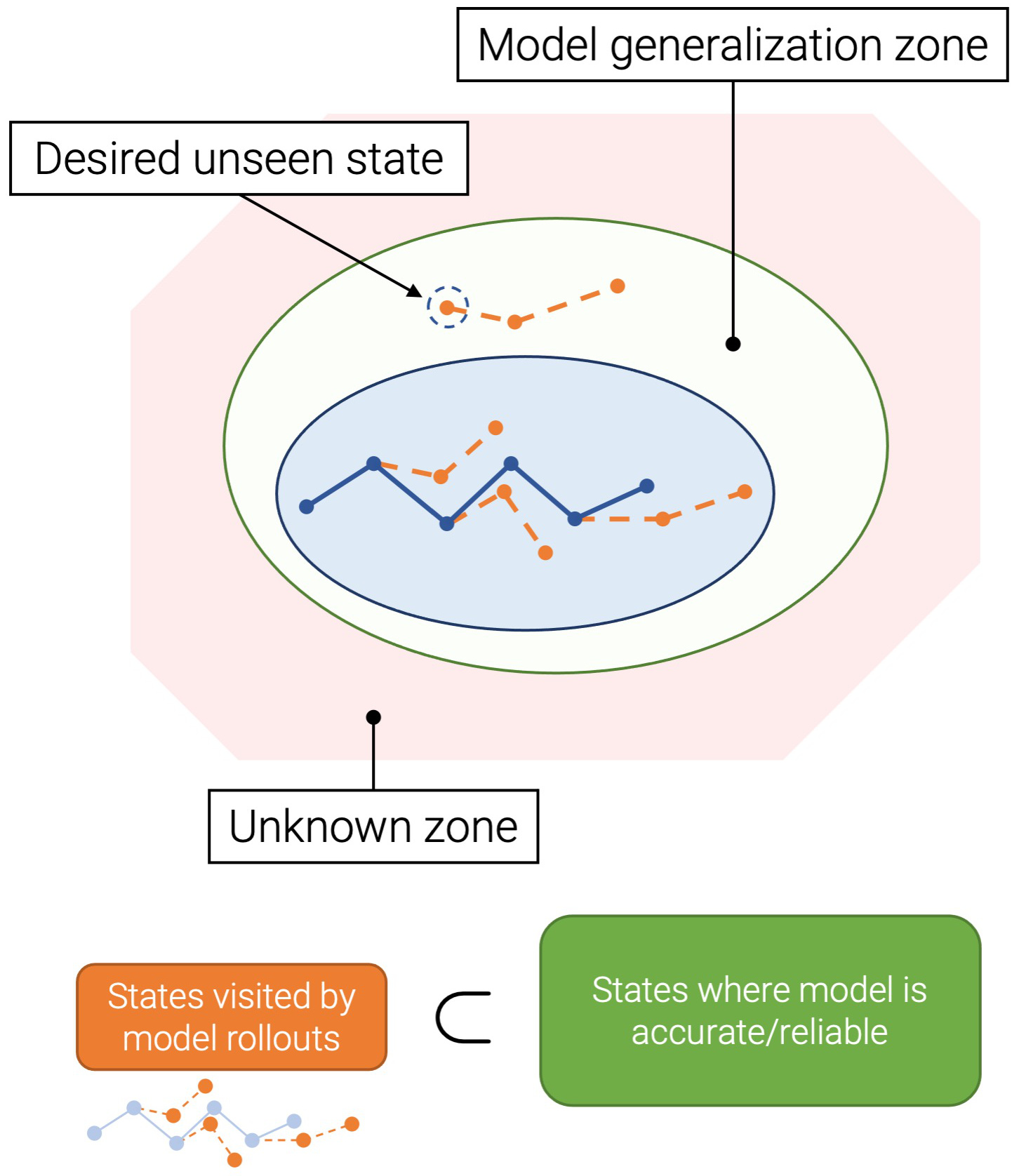
Figure 1: We hypothesize that there exists a ‘green zone’ of model generalization that is not covered by the extent of model rollouts with short horizons (innermost blue zone). We propose a strategy to find such states and show that this leads to improved offline RL performance and lower conservative Q-value estimates.

Offline reinforcement learning (offline RL, batch RL) (Levine et al., 2020; Lange et al., 2012; Fujimoto et al., 2019) is a uniquely challenging problem due to the offline nature of data being used to learn policies, without any new environment interactions. It has also gained relevance due to the increasingly large amounts of offline data available for gleaning useful behaviors without the need for training from scratch. Offline RL has been applied broadly – in robotics, machinery and healthcare (Levine et al., 2020; Wang et al., 2018; Kalashnikov et al., 2021; Zhan et al., 2022), where exploration is costly and often dangerous.

Offline RL algorithms have an inherent risk trade-off – better performance beyond that of the observed behaviors in offline data comes with higher uncertainty in value estimates from states and actions far away from seen data. Traditional offline RL methods realize this trade-off by either penalizing deviation from observed behavior (Fujimoto et al., 2018; Yu et al., 2020) or by conservatively estimating values for unseen actions such as in Conservative Q-Learning (CQL (Kumar et al., 2020)). While model-free methods have prescribed ways for dealing with unseen actions, model-based offline RL methods (Yu et al., 2021; Kidambi et al., 2020; Yu et al., 2020) utilize a model of the transition dynamics and reward in order to leverage generalization to unseen states in addition to unseen actions. However, model-based offline RL methods are not able to meet such expectations of generalization to unseen state due to a combination of two limiting factors – (i) value estimates via model-based value expansion (MVE (Palenicek et al., 2022; Feinberg et al., 2018)) are made starting from seen states alone, ignoring those unseen states where learned estimators may have low error, and (ii) the rollout horizon for model-based value expansion is typically very short due to compounding errors in long horizon future predictions.

We hypothesize that expanding model-based value estimation to carefully selected unseen states will improve state-action value estimation at unseen states while maintaining the conservative bias for unseen quantities (states as well as actions) as prescribed in prior works such as CQL (Kumar et al., 2020) and COMBO (Yu et al., 2021). We design an unseen state generation strategy with a propose and filter strategy – (i) candidate unseen states proposals are generated via value-informed perturbations to seen states, (ii) candidates that have too high estimated uncertainty (likely to have high model and value estimation error) or too low epistemic uncertainty (likely to be too similar to seen states and less informative) are discarded.

We present empirical evidence of improved performance on the D4RL benchmark (Fu et al., 2020) and several analyses of the mechanism of action of our method. We show the reliability of our epistemic uncertainty estimation is predicting true model error, demonstrating that it is more suitable than aleatoric uncertainty estimators that have been shown to have poor correlation with true model error (Yu et al., 2021). We study the importance of our value-informed perturbations by (i) measuring the informativeness of value-informed state perturbation as opposed to perturbing states in random directions and (ii) ablating the direction of value-informed perturbations. Finally, we present an analysis of average dataset Q-value, the key metric used in prior work (COMBO (Yu et al., 2021)) for offline hyperparameter selection, and demonstrate that our perturb and filter strategy leads to significantly lower average dataset Q-value estimates on top of COMBO (used as a baseline) – hinting that the mechanism of action for improved performance may be in decreased Q-value estimates in the face of conservative penalties.

2 Related Work

Offline or Batch Reinforcement Learning is the problem of learning optimal quantities (values or policies) from a fixed set of experiences or data, with its roots in fitted value and Q iteration (Gordon, 1995; Riedmiller, 2005) and has recently gained popularity due to the success of powerful function approximators such as deep neural networks in learning policies, values, rewards and dynamics (Levine et al., 2020; Yu et al., 2020, 2021; Kidambi et al., 2020). Offline RL is distinct from imitation learning as the latter assumes expert demonstrations as offline data without reward labels, whereas offline RL assumes known reward labels, allowing for use of sub-optimal or non-expert data. Offline RL datasets such as D4RL (Fu et al., 2020) and NeoRL (Qin et al., 2021) are prominent benchmarks for evaluating and comparing offline RL methods. We use environments from D4RL in this chapter for evaluating our method.

Unlabeled Data in Offline RL: Offline RL assumes that the fixed dataset consists of tuples of state, action, next state and reward. However, unlabeled data i.e. without reward labels is often plentiful and an the question of how to leverage such data to improve Offline RL with a typically smaller labeled dataset is an important question. Setting the reward of unlabeled data to zero has been shown to be a simple and effective strategy to leverage this data (Yu et al., 2022). Intuitively, this is reasonable to expect as Q-values from reward labeled states will propagate to unlabeled states during learning of a Q-function with temporal difference.

Conservative Q-Learning (CQL): A number of works have used or adapted the method of learning conservative Q estimates by penalizing the estimated value of unseen actions while pushing up value of seen actions in the offline dataset (Kumar et al., 2020). Yu et al. (2021) is a model-based approach that combines CQL (Kumar et al., 2020) with model-based reinforcement learning by additionally penalizing the estimated values of states actions in model rollouts.

Model-based Offline RL: COMBO (Yu et al., 2021), MOREL (Kidambi et al., 2020) are model-based offline RL approaches that use the approximate MDP induced by a learned dynamics model network with a conservative objective. As previously mentioned, Yu et al. (2021) uses CQL by penalizing estimated value of state-actions visited during model rollouts stating from seen states, while Kidambi et al. (2020) defines their induced MDP in a conservative manner by stopping any model rollouts that fall into states with high uncertainty as measured by model ensemble disagreement. COMBO Yu et al. (2021) expressly avoids uncertainty estimation citing its inaccuracy in some settings. There are two key differences w.r.t COMBO – (i) we use epistemic uncertainty estimation and show its correlation with true model error, whereas COMBO demonstrated the poor correlation of aleatoric uncertainty estimation with true model error; (ii) we do not re-introduce uncertainty in the manner COMBO recommended to avoid – we use uncertainty to filter unseen states used for starting model rollouts as opposed to using it as a reward penalty (as in MOPO (Yu et al., 2020)).

Adversarial Unseen State Augmentation: Zhang & Guo (2021) is a model-free online RL approach that proposes adversarial states as data augmentation for policy updates via multiple gradient steps in state space. This is similar to our approach that proposes unseen states via multiple gradient updates in the state space of the Q-value estimate. Other than the difference of objective for computing the gradient, there are also two additional differences between Zhang & Guo (2021) and our approach – (1) we use both the positive and negative gradient direction for proposing unseen states and find that both are jointly more useful than one direction alone, whereas Zhang & Guo (2021) is purely adversarial (minimizing their objective with gradient descent), and (2) Zhang & Guo (2021) keep the sampled action fixed while minimizing their adversarial objective while we use the differentiability of the parameterized policy to sample new actions.

3 Preliminaries

In this section, we briefly touch upon Offline Reinforcement Learning (RL) and the baseline COMBO (Yu et al., 2021) that we build upon and compare with in our analysis.

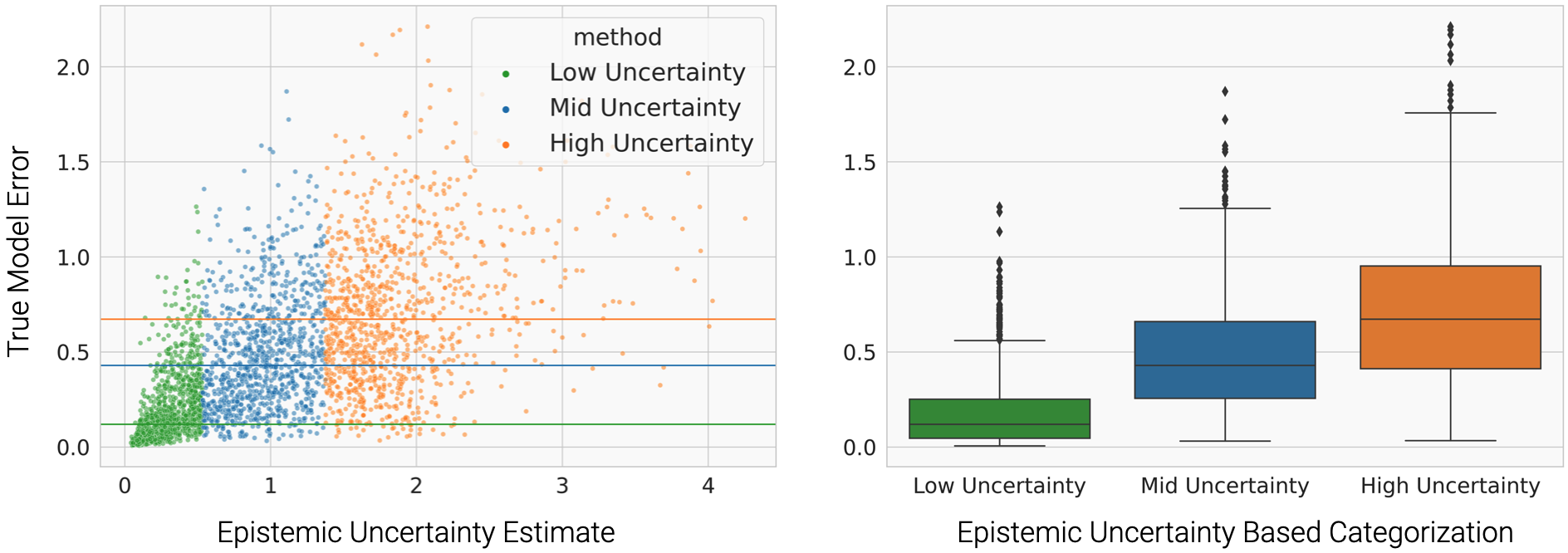
Figure 2: (Left) Relationship between epistemic uncertainty estimated using ensemble disagreement and true model error i.e. the mean absolute difference between model next state and reward predictions and true quantities, for the Adroit Pen manipulation task and Human demonstrations dataset. Each point corresponds to a state obtained by model rollouts from a perturbed state in Algorithm 2. Horizontal lines measure medians for respective uncertainty category. (Right) Box plot of true model error aggregated for each uncertainty category. The two boundaries for the categories are the 0.25 and 0.75 quantile uncertainty estimates on the seen states in the offline dataset. The states filtered into the Mid Uncertainty class are used for unseen state augmentation.

Offline RL. In Offline Reinforcement Learning, a fixed dataset of interactions $\mathcal{D}:={(s,a,r,s^{\prime})}$ is provided for finding the best possible policy without any environment interactions (i.e. without “online” interactions). Since we only deal with simulated environments, the policy found by an algorithm is evaluated with online evaluation.

Model-based Offline RL. COMBO (Yu et al., 2021) is a model-based offline RL algorithm that extends the concept of conservative Q-learning in CQL (Kumar et al., 2020) to model-generated predictions. Algorithm 1 depicts the model-based RL algorithm used by COMBO. First, an initial model fitting stage is executed where the reward and dynamics model is trained with maximum likelihood estimation (MLE) on the offline data. Second, policy and critic learning happens over a fixed number of training epochs where the data used for policy training is obtained by means of branched rollouts. Branched rollouts are inherited from the model-based algorithm MOPO (Yu et al., 2020) (which COMBO uses as a foundation), where a batch of initial states are sampling from the offline dataset and used to generate model-rollouts up to a fixed horizon $H$ using actions sampled from a rollout policy $\mu(\cdot\mid s)$ (typically the same as $\pi$ or sometimes a uniform over actions policy) and next states sampled from the learned dynamics model (almost always Gaussian with mean and variance predictions). Then, the policy and critic are updated using this rollout data.

The conservative Q-value update used by COMBO is as follows. Here, $d_{f}$ is an interpolation defined by (Yu et al., 2021) as $d_{f}(s,a):=fd(s,a)+(1-f)d^{\mu}_{{{\color[rgb]{1,0,0}M_{\phi}}}}(s,a)$; where $d$ is the empirical sampling distribution from the offline dataset $\mathcal{D}$.

$$\hat{Q}^{k+1} \leftarrow\mathop{\mathrm{argmin}}_{Q}\mathcal{L}_{\textrm{TD}}+\beta\cdot\mathcal{L}_{\textrm{CQL}}$$

$$\mathcal{L}_{\textrm{TD}} :=\mathop{\mathbb{E}}_{(s,a,s^{\prime})\sim d_{f}}\Bigg{[}\bigg{(}\bigg{(}r(s,a)$$

$$\phantom{AAA}+\gamma\mathop{\mathbb{E}}_{a^{\prime}\sim\hat{\pi}^{k}\left(a^{\prime}\mid s^{\prime}\right)}\left[\hat{Q}^{k}\left(s^{\prime},a^{\prime}\right)\right]\bigg{)}-Q(s,a)\bigg{)}^{2}\Bigg{]}$$

$$\mathcal{L}_{\textrm{CQL}} :=\mathop{\mathbb{E}}_{s\sim d_{{{\color[rgb]{1,0,0}M_{\phi}}},\pi},a\sim\pi}\left[Q(s,a)\right]-\mathop{\mathbb{E}}_{(s,a)\sim\mathcal{D}}\left[Q(s,a)\right]$$ (1)

The right hand term in Equation 1 is further used for offline tuning of hyperparameters in COMBO – a trait that we inherit when using COMBO as a baseline. Conservative Q-value estimation is applied to all rollout data (i.e. Q-values are pushed down for unseen states predicted by the model). This implies that while Q-value propagation does occur for unseen states found by model rollouts, they are down-weighted proportional to the coefficient $\beta$ in the above equation (1). This implies that when we do find unseen states (in Section 4) in regions not visited by branched rollouts, they will also bear the same conservative penalty.

Algorithm 1 Model-based Offline RL with COMBO (Yu et al., 2021)

  Input:Offline dataset $\mathcal{D}$, parametrized policy and critic $\pi_{\theta}$, $Q_{\theta}$

  Input:Parametrized dynamics model $\mathcal{P}_{{{\color[rgb]{1,0,0}\phi}}}$

  Input:Rollout policy $\mu(\cdot\mid s)$, horizon $H\in\mathbb{N}$

  Split $D$ into train, val splits and optimize $\mathcal{P}_{{{\color[rgb]{1,0,0}\phi}}}$ until convergence on val set;

  for $i=1$ to $n_{\textrm{epochs}}$ do

     $\mathcal{D}_{0}\leftarrow$ Sample a batch of start states from $\mathcal{D}$;

     $\hat{\mathcal{D}}\leftarrow$ Collect model rollouts with $\mu,\mathcal{P}_{{{\color[rgb]{1,0,0}\phi}}}$ up to $H$ starting from states in $\mathcal{D}_{0}$;

     Fit $Q_{\theta}$ with a conservative objective using both $\mathcal{D}$ and $\hat{\mathcal{D}}$;

     Update policy $\pi_{\theta}$ using estimated $Q_{\theta}$ values on $\hat{\mathcal{D}}$;

  end for

4 Approach

In this section, we first motivate our method by highlighting the limitations of using branched model rollouts along with short model prediction horizons. This raises the question of how to find unseen states for model rollouts in a manner that is accurate (unseen states have low model error during rollouts) and useful (leads to better downstream task performance). To achieve this, we introduce a simple propose and filter strategy for finding unseen states – a proposal stage where a seen state is perturbed and a filter stage where states having estimated uncertainty too low or too high are discarded. We then propose two perturbation functions for obtaining unseen state proposals – one that perturbs randomly uniformly in any direction and a second that perturbs along the positive and negative direction of the Q-value gradient w.r.t states.

Limitations of Short Horizon Branched Rollouts. In offline-RL, branched model rollouts utilize every state in the seen dataset for performing rollouts i.e. sequential model next state predictions given a behavior policy, up to horizon $H$. Such unseen state predictions populate the rollout buffer and along with seen states, they are used for Q-learning using temporal difference and conservative objectives (CQL Kumar et al. (2020)). Ideally, to fully exploit the learned model, all states where the model has low uncertainty should be included in the rollout buffer for Q-learning. However, this may not be the case as there is no guarantee that the states visited by $H$ horizon model rollouts will visit all possible states where the model has low uncertainty i.e. states where the learned dynamics and reward model generalizes. We will show in our experiments that exploiting such unseen states consistently leads to lower Q-value estimates.

Start State Augmentation. In order to maximize coverage of states where the learned dynamics and reward model generalize to, as measured by estimated uncertainty, we propose an augmentation strategy that uses a mixture of seen and unseen states as starting points to perform model rollouts. Given a batch of $n_{\textrm{start}}$ states sampled from the offline dataset, we control the fraction of this batch to replace with unseen states as $f_{\textrm{augment}}\in[0,1]$. We find that $f_{\textrm{augment}}=0.5$ works well in practice. Note that $f_{\textrm{augment}}=0$ reduces to a no augmentation baseline.

Perturb and Filter with Q-gradients. Algorithm 2 details the subroutine, referred to as PnF-Qgrad , that takes as input a batch of states sampled from the offline dataset and produces a set of potentially unseen states via a perturb and filter strategy. First, a set of candidate state proposals are generated by taking $n_{\textrm{steps}}$ gradient steps using the Q-value gradient w.r.t state input, with a step size uniformly sampled from $(-\delta_{\textrm{max}},\delta_{\textrm{max}})$ i.e. with positive as well as negative directions, and fixed across gradient steps. Next, uncertainty cut-off points $u_{\textrm{lower}},u_{\textrm{upper}}$, computed using the $0.25$ and $0.75$ quantile uncertainty values of seen data, are used for filtering out states that lie outside of the range $(u_{\textrm{lower}},u_{\textrm{upper}})$. This process is repeated until the desired number of augmented states $n_{\textrm{augment}}$ have been obtained. The while loop typically runs for just one iteration in most of our hyperparameter choices.

Uncertainty Estimator. We tested 3 types of uncertainty estimators: (1) ensemble disagreement via max 2-norm deviation from mean across ensemble (used in MOPO implementation by (Qin et al., 2021)), (2) maximum 2-norm of standard deviation across ensemble from (used by MOPO (Yu et al., 2020)) and (3) standard deviation of mean predictions over ensemble. Here, the first and third estimators approximate epistemic uncertainty while the second approximates aleatoric uncertainty. We found (1) and (3) to overall work well in practise and we select (1) as our choice of uncertainty estimator for all of our experiments. We exclude MOREL’s discrepancy based uncertainty (Kidambi et al., 2020), as we found it to be similar to (1) in form and practice. Figure 2 (left) shows the correlation between epistemic uncertainty (using (1)) and true model error for the Adroit Pen manipulation task with the Human demonstrations dataset. Figure 2 (right) demonstrates our strategy for filtering states – defining a minimum and maximum threshold based on the 0.25 and 0.75 quantile uncertainty values computed on the seen states in the offline dataset.

Ablations. In addition to using the Q-value gradient for generating state proposals, we also test an ablation of our method named PnF-Random , that substitutes the Q-value gradient in Algorithm 2, 11 with a unit vector sampled uniformly randomly on a hypersphere. In order to prevent random walks, we fix $n_{\textrm{steps}}$ to $1$ for this ablation so that the augmented states are solely a result of a single perturbation per direction. We find that the Q-gradient produces more informative state proposals after filtering than this PnF-Random , as measured by final policy performance on tested offline RL benchmarks.

Algorithm 2 PnF-Qgrad : Value-aware unseen state augmentation

  Input:Input state batch $\mathcal{D}_{\textrm{batch}}\subseteq\mathcal{D}$, parametrized Q-network $Q_{\theta}$, policy network $\pi_{\theta}$

  Input:State-dependent uncertainty estimation function $\xi:\mathcal{S}\rightarrow\mathbb{R}$

  Input:Number of steps of perturbation $n_{\textrm{steps}}$, maximum step size $\delta_{\textrm{max}}$

  Input:Desired number of augmented states $n_{\textrm{augment}}$ to fill $\mathcal{D}_{\textrm{augment}}$

  Initialize $\mathcal{D}_{\textrm{augment}}\leftarrow\emptyset$ and $U_{0}:=\{\xi(s):s\in\mathcal{D}_{\textrm{batch}}\}$;

  Initialize $u_{\textrm{lower}}$, $u_{\textrm{upper}}$ as $0.25$-quantile and $0.75$-quantile of $U_{0}$ respectively;

  while $\left|\mathcal{D}_{\textrm{augment}}\right|<n_{\textrm{augment}}$ do

     $\overline{\mathcal{D}}_{0}\leftarrow\{s:(s,a,r,s^{\prime})\in\mathcal{D}_{\textrm{batch}}\}$;

     Sample $\eta_{s}\sim U(-\delta_{\textrm{max}},\delta_{\textrm{max}})\forall s\in\overline{\mathcal{D}}_{0}$;

     for $i$ from $1$ to $n_{\textrm{steps}}$ do

        $\overline{\mathcal{D}}_{i}\leftarrow\{\overline{s}:\overline{s}\leftarrow s+\eta_{s}\cdot\nabla_{s}Q_{\theta}(s,\pi_{\theta}(s))\}$;

     end for

     $\overline{\mathcal{D}}_{\textrm{all}}\leftarrow\bigcup_{i=1}^{n_{\textrm{steps}}}\overline{\mathcal{D}}_{i}$;

     $\overline{\mathcal{D}}_{\textrm{filtered}}\leftarrow\{s:\xi(s)>u_{\textrm{lower}}\textrm{ and }\xi(s)<u_{\textrm{upper}}\ \forall\boldsymbol{s}\in\overline{\mathcal{D}}_{\textrm{all}}\}$;

     $\mathcal{D}_{\textrm{augment}}\leftarrow\mathcal{D}_{\textrm{augment}}\bigcup\overline{\mathcal{D}}_{\textrm{filtered}}$ ;

     If $\left|\mathcal{D}_{\textrm{augment}}\right|>n_{\textrm{augment}}$, subsample uniformly to keep $n_{\textrm{augment}}$ elements;

  end while

  Input:Offline dataset $\mathcal{D}$, parametrized policy and critic $\pi_{\theta}$, $Q_{\theta}$

  Input:Parametrized dynamics model $\mathcal{P}_{{{\color[rgb]{1,0,0}\phi}}}$

  Input:Rollout policy $\mu(\cdot\mid s)$, horizon $H\in\mathbb{N}$

  Input:Fraction of start state batch to augment $f_{\textrm{augment}}\in[0,1]$

  Split $D$ into train, val splits and optimize $\mathcal{P}_{{{\color[rgb]{1,0,0}\phi}}}$ until convergence on val set;

  for $i=1$ to $n_{\textrm{epochs}}$ do

     $\mathcal{D}_{\textrm{start}}\leftarrow$ Sample a batch of $n_{\textrm{start}}$ start states from $\mathcal{D}$;

     $\mathcal{D}_{\textrm{start}}\leftarrow$ Augment $n_{\textrm{augment}}:=\left\lfloor f_{\textrm{augment}}\cdot n_{\textrm{start}}\right\rfloor$ states using Algorithm 2;

     $\hat{\mathcal{D}}\leftarrow$ Collect model rollouts with $\mu,\mathcal{P}_{{{\color[rgb]{1,0,0}\phi}}}$ up to $H$ starting from states in $\mathcal{D}_{\textrm{start}}$;

     Fit $Q_{\theta}$ with a conservative objective using both $\mathcal{D}$ and $\hat{\mathcal{D}}$;

     Update policy $\pi_{\theta}$ using estimated $Q_{\theta}$ values on $\hat{\mathcal{D}}$;

  end for

Algorithm 3 Model-based Offline RL with State Augmentation

5 Experiments

In this section, we perform empirical analyses to answer the following questions: (1) Does our COMBO PnF-Qgrad method lead to improvemenet in offline RL performance over a baseline? (2) Does the Q-gradient direction matter for perturbation, when compared to performance of a PnF-Random baseline? (3) Does the sign of the perturbation (i.e. ascending or descending the Q-gradient) matter for performance? and (4) What are the distance characteristics of the unseen states found with PnF augmentation as opposed to the unseen states visited by model rollouts in the baseline?

5.1 Performance on D4RL Environments and Datasets

We use COMBO (Yu et al., 2021) as a foundation on top of which we implement our method PnF-Qgrad . We use the open source PyTorch implementation of COMBO by (Qin et al., 2021). Our method requires specification of the following additional hyperparameters.

1. $n_{\textrm{steps}}$: Number of gradient descent or ascent steps in Algorithm 2. We use the range $\{1,2,4,8\}$ to pick the best value.

2. $\delta_{\textrm{max}}$: Maximum value of step size $\eta_{s}$ in Algorithm 2. We use the (logarithmic) range $\{1.0E-5,5.0E-5,1.0E-4,5.0E-4,1.0E-3,5.0E-3,1.0E-2,5.0E-2,1.0E-1,0.5\}$ to pick the best value.

3. $f_{\textrm{augment}}$: Fraction of batch of start states to augment in Algorithm 3. We use the range $\{0.5,0.9,1.0\}$ to pick the value, with the mimunum fraction of $0.5$ guaranteeing that at least half of the batch is augmented.

We first compare PnF-Qrad performance to COMBO on several offline RL environments from the D4RL benchmark (Fu et al., 2020). We refer to our method as COMBO PnF-Qgrad to emphasize that COMBO is the base algorithm on top of which we perform unseen state augmentation. Similarly, we refer to our method with random perturbation directions as COMBO PnF-Random .

In D4RL, a task (e.g. Pen-v1 Human) is specified by a choice of environment (e.g. Adroit Pen environment) and a choice of dataset (e.g. Human demonstrations). Figure 3 evaluates COMBO , COMBO PnF-Qgrad and COMBO PnF-Random on two types of D4RL tasks – the Maze2D family of tasks that have three different environments corresponding to varying maze grid sizes (Umaze, Medium, Large). We find that on the Pen-v1 Human task consisting of 4950 time steps of human demonstrations, COMBO PnF-Qgrad significantly outperforms baselines. However, on the Pen-v1 Cloned and Pen-v1 Expert tasks, we find that all methods including baselines perform poorly. In the Maze2D tasks, we find an improvement over COMBO for both COMBO PnF-Qgrad and COMBO PnF-Random on the Maze2D-v1 Large task. COMBO PnF-Random performs poorly on the Maze2D-v1 Medium and Maze2D-v1 Umaze tasks where COMBO and COMBO PnF-Qgrad perform comparably.

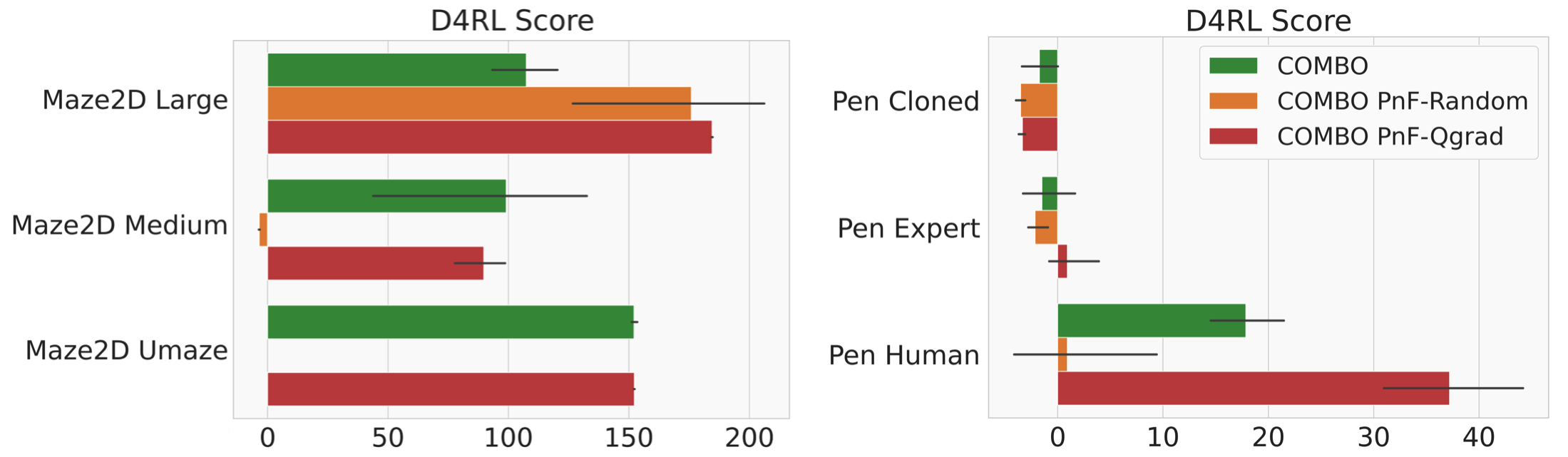
Figure 3: Evaluation on two sets of D4RL offline datasets, the Maze2D environment with varying maze sizes (left) and Adroit Dextrous Hand Manipulation - Pen Environment with varying dataset types (right). The Maze2D dataset contain a little under $4$ million time steps. The Pen-v1 Expert and Pen-v1 Cloned datasets contain close to $\sim 495000$ time steps, whereas the Pen-v1 Human dataset contains $4950$ time steps. Hyperparameters are tuned on Maze2D-v1 Medium for the Maze2D tasks and Pen-v1 Human for the Adroit Pen tasks.

Hyperparameter Sensitivity In Table 1, we compare COMBO PnF-Qgrad , COMBO (our implementation using (Qin et al., 2021) and the reported performance by Yu et al. in (Yu et al., 2021). Due to computational resource constraints, we tune hyperparameters on a single task – the Walker2D-v2 Medium-Replay task, while evaluating on all other tasks. We find that, while we do observe statistically significant improvement in performance on the same environment where hyperparameter values were tuned, we don’t see a complete replication of this trend when transferring hyperameters to other tasks. We suspect that this sensitivity is a result of the varying distribution and distance between states in each dataset and environment, as these will affect the perturbation magnitude in our method PnF-Qgrad (e.g. value of $\delta_{\textrm{max}},n_{\textrm{steps}}$).

Average Dataset Q-value In Figure 4, we measure the average dataset Q-value, a quantity important for not only selecting hyperparameters in an offline manner, but one which has shown to indicate online evaluation performance. COMBO (Yu et al., 2021) has shown lower average dataset Q-values lead to more conservative Q-value estimates i.e. preventing any overestimation of Q-values, and higher online evaluation performance (D4RL score). We find that throughout the 500 epochs of policy training, average dataset Q-value is significantly lower for COMBO PnF-Qgrad in comparison to COMBO. Further, in Figure 5, we see that this trend holds when reducing the size of the dataset, despite the performance of the two being comparable at lower dataset sizes. This suggests that conservative Q-value estimation is an important mechanism of action for our proposed method in contributing to better online evaluation performance.

Table 1: D4RL Score mean and standard error over 6 random seeds for (left to right) COMBO (reported in (Yu et al., 2021)), the implementation of COMBO by (Qin et al., 2021) that we use and our proposed PnF-Qgrad method. PnF-Qgrad requires tuning of the hyperparameters $\delta_{\textrm{max}},n_{\textrm{steps}},f_{\textrm{augment}}$ which are sensitive to both datasets and environments. We tune these hyperparameters on the Walker2D-v2 Medium-Replay dataset, according to the offline tuning guidelines from (Yu et al., 2021; Kumar et al., 2021), and report online evaluation performance of the selected hyperparameters across all other environments and datasets. $*$ indicates tuned on Walker2D-v2 Medium-Replay.

Dataset type	Environment	COMBO (Yu et al.)	COMBO	COMBO PnF-Qgrad*
random	halfcheetah	$38.8\pm 3.7$	$14.5\pm 6.4$	$-1.5\pm 0.5$
random	hopper	$17.9\pm 1.4$	$4.7\pm 1.8$	$4.6\pm 2.6$
random	walker2d	$7.0\pm 3.6$	$7.6\pm 1.4$	$5.1\pm 1.8$
medium	halfcheetah	$54.2\pm 1.5$	$62.6\pm 1.3$	$41.2\pm 4.5$
medium	hopper	$97.2\pm 2.2$	$61.0\pm 0.4$	$51.6\pm 15.5$
medium	walker2d	$81.9\pm 2.8$	$34.2\pm 0.0$	$70.4\pm 2.0$
medium-replay	halfcheetah	$55.1\pm 1.0$	$53.0\pm 6.1$	$41.0\pm 3.8$
medium-replay	hopper	$89.5\pm 1.8$	$41.3\pm 11.3$	$34.5\pm 19.1$
medium-replay	walker2d	$56.0\pm 8.6$	$32.1\pm 25.7$	$\mathbf{70.9\pm 4.3}$
med-expert	halfcheetah	$90.0\pm 5.6$	$37.6\pm 0.0$	$86.4\pm 3.5$
med-expert	hopper	$111.1\pm 2.9$	$34.6\pm 30.4$	$18.7\pm 4.6$
med-expert	walker2d	$103.3\pm 5.6$	$48.3\pm 68.0$	$54.2\pm 25.5$

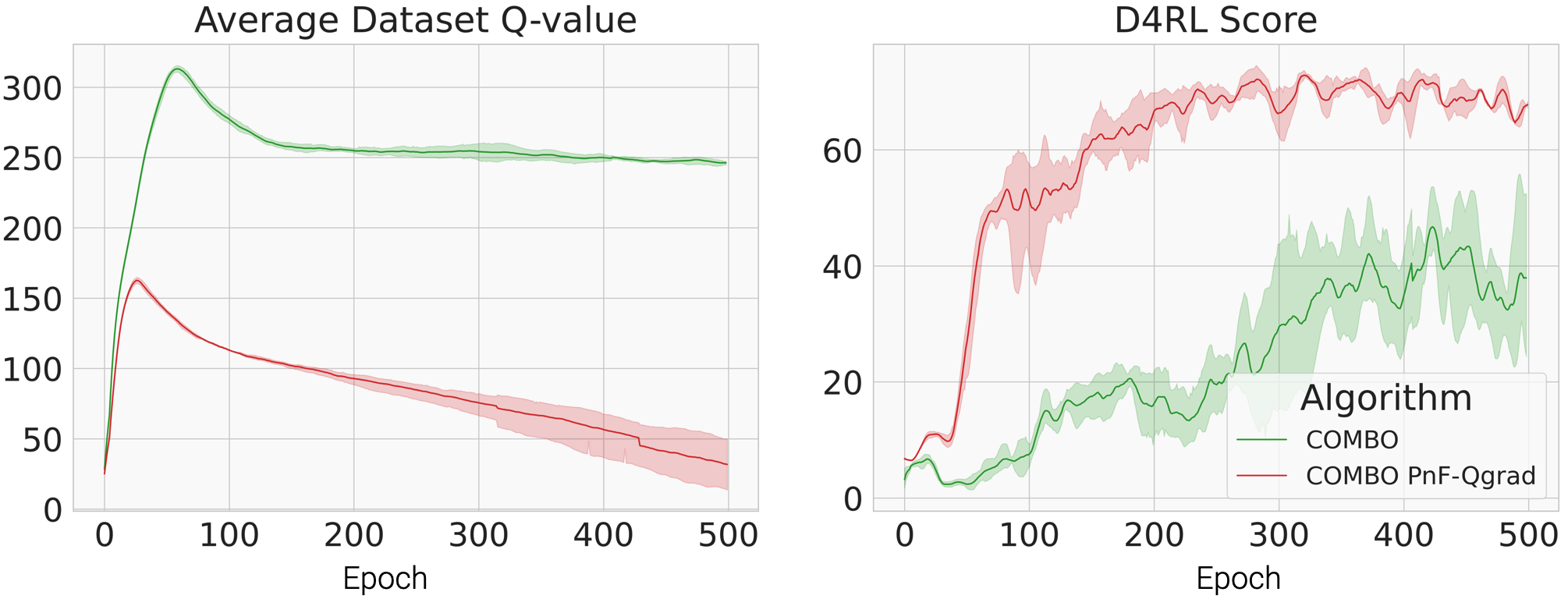
Figure 4: Average dataset Q-value (left) and D4RL score (right) for the Walker2d-v2 Medium-Replay task over 6 random seeds. The training curve is for 500 epochs of the policy update phase that occurs after an initial phase of fitting a model to the offline dataset. A consistently and significantly lower overall average dataset Q-value is obtained for COMBO PnF-Qgrad in comparison to the COMBO baseline. COMBO (Yu et al., 2021) advocates for lower average dataset Q-values as they prevent overestimation of Q-value for unseen states and actions, while also being strongly linked to higher online evaluation performance (D4RL score). We observe a similar result i.e. lower average dataset Q-values for COMBO PnF-Qgrad lead to better D4RL score.

In Figure 5, we also demonstrate the effect of reducing dataset size for the Walker2D-v2 Medium-Replay task. We reduce dataset size by selecting a contiguous sub-arrays from the front of the original dataset given a fraction (e.g. fraction $0.5$ takes the first half of the dataset). While fractions of $0.5$ and smaller rapidly reduce performance and make them comparable across methods, we observe that the average dataset Q-value remains significantly lower for COMBO PnF-Qgrad in comparison to COMBO.

Figure 5: D4RL score (left) and average dataset Q-value (right) for varying dataset size fractions for the Walker2D-v2 Medium-Replay task. Each dataset fraction corresponds to a contiguous subarray taken from the front of the original dataset. We observe significantly lower average dataset Q-values but comparable D4RL scores for COMBO PnF-Qgrad versus COMBO as the dataset size reduces.

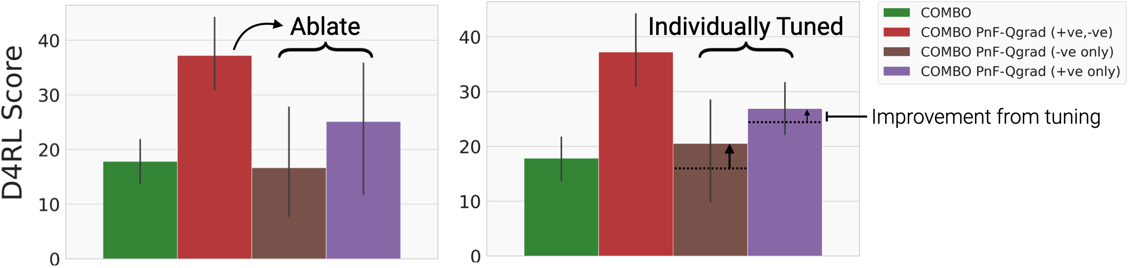
Figure 6: D4RL Score comparison on Pen-v1 Human task over 6 random seeds of ablations of PnF-Qgrad that use positive-only step size along Q-gradient (i.e. $\eta_{s}\sim U(0,\delta_{\textrm{max}})$ in Algorithm 2), and negative-only step size along Q-gradient i.e. (i.e. $\eta_{s}\sim U(-\delta_{\textrm{max}},0)$ in Algorithm 2). (left) Ablations for positive-only and negative-only inherit the hyperparameter values ($n_{\textrm{steps}},f_{\textrm{augment}},\delta_{\textrm{max}}$) from PnF-Qgrad (positive, negative) (red bar). (right) Each ablation is individually tuned to obtain best value of hyperparameters $n_{\textrm{steps}},f_{\textrm{augment}},\delta_{\textrm{max}}$.

Figure 7: Histograms of distance of visited unseen states from seen dataset computed using L2 distance from nearest neighbor in seen dataset (X-axis) for the Pen-v1 Human dataset. Unseen states in the COMBO baseline are obtained by model rollouts from seen states, whereas unseen states from PnF-Qgrad and PnF-Random are obtained using model rollouts starting from augmented states using Algorithm 2 and their respective choice of perturbation directions. Rollout horizon values are (left to right) $1,5,10$. PnF-Qgrad uses $\delta_{\textrm{max}}=0.001$, $n_{\textrm{steps}}=4$ and PnF-Random uses $\delta_{\textrm{max}}=0.1$, $n_{\textrm{steps}}=1$, which were the best hyperparameter values selecting after tuning. Dark colored full length vertical lines correspond to median of respective distribution.

5.2 Sign of Perturbation

In Algorithm 2, we choose the step size $\eta_{s}\in U(-\delta_{\textrm{max}},\delta_{\textrm{max}})$ for a given direction $\nabla_{s}Q_{\theta}(s,\pi_{\theta}(s))$. In order to verify that both positive and negative step sizes for perturbation along this direction are important for good performance, we evaluate two ablations that use either a positive-only step size or a negative-only step size, using the Pen-v1 Human task. We refer to COMBO PnF-Qgrad (+ve, -ve) as our original method that samples $\eta_{s}\in U(-\delta_{\textrm{max}},\delta_{\textrm{max}})$, COMBO PnF-Qgrad (+ve-only) as the positive-only ablation that samples $\eta_{s}\in U(0,\delta_{\textrm{max}})$ and COMBO PnF-Qgrad (+ve-only) as the negative-only ablation that samples $\eta_{s}\in U(-\delta_{\textrm{max}},0)$. Figure 6 highlights our findings in two settings. First, we use inherit the hyperparameter values for each ablation from the COMBO PnF-Qgrad (+ve, -ve). In this setting, we find that performance is immediately lowered for both ablations, indicating that either both positive and negative step sizes matter, or that the ablations may need to be individually tuned. Second, we eliminate one of the possibilities by individually tuning hyperparameter values for both ablations, where performance is slightly improved over the un-tuned methods, while still having lower performance than COMBO PnF-Qgrad (+ve, -ve). As a result, we find that it is important to perturb along the positive as well as negative direction of Q-value gradient for best performance.

5.3 Distribution of Perturbation Distance

In order to understand the impact of our studied perturbations on the distance of augmented unseen states from seen states, we plot a histogram of nearest neighbor distances of every unseen state (w.r.t seen states in the entire offline dataset) visited by Algorithm 3 (for PnF-Qgrad and PnF-Random ) and Algorithm 1 (COMBO). For each algorithm, the set of unseen states are an aggregation of all states visited during model rollouts. For Algorithm 3, we set the fraction of model rollouts that occur from unseen states, $f_{\textrm{augment}}$, to $1.0$ We expect that any perturbation based unseen state augmentation has the potential to visit states in model rollouts that are far away from any nearest seen state.

Figure 7 plots these histograms for PnF-Qgrad , PnF-Random and COMBO on the Pen-v1 Human task with rollout horizon values in $\{1,5,10\}$. For PnF-Qgrad , we set $\delta_{\textrm{max}}=0.001,n_{\textrm{steps}}=4$, which are the tuned values of these hyperparameters for this task. Similarly, for PnF-Random , we set $\delta_{\textrm{max}}=0.1,n_{\textrm{steps}}=1$ (note that for PnF-Random , $n_{\textrm{steps}}$ is always set to $1$ as multiple gradient steps are not necessary for a random perturbation direction). We find that despite the low value of $\delta_{\textrm{max}}$, PnF-Qgrad is able to find unseen state augmentations that produce model rollout states with farther nearest neighbor L2 distance than the model rollouts states visited by no augmentation (COMBO baseline). This is in comparison to PnF-Random , which has overall distribution of distances similar to no augmentation (despite the higher $\delta_{\textrm{max}}$). This indicates that PnF-Qgrad is able to find unseen states farther from seen data while still passing through uncertainty filter, whereas random perturbation are not able to do the same.

6 Conclusion

In this paper, we addressed the limitations of model-based offline reinforcement learning methods in their ability to find and utilize unseen states for Q-value estimation. We proposed an unseen state augmentation strategy that is able to find states that are far away from the seen states in the offline dataset, have low estimated epistemic uncertainty and which lead to overall lower Q-value estimates and better performance in several offline RL tasks. We present a value-informed perturbation strategy that uses the positive and negative Q-value gradient direction to generate unseen state proposals; and find improved performance compared to an ablation that perturbs uniformly randomly in all directions and ablations that use the positive or negative Q-value gradient direction alone.

References

- Feinberg et al. (2018) Feinberg, V., Wan, A., Stoica, I., Jordan, M. I., Gonzalez, J. E., and Levine, S. Model-based value estimation for efficient model-free reinforcement learning. arXiv preprint arXiv:1803.00101, 2018.
- Fu et al. (2020) Fu, J., Kumar, A., Nachum, O., Tucker, G., and Levine, S. D4rl: Datasets for deep data-driven reinforcement learning. arXiv preprint arXiv:2004.07219, 2020.
- Fujimoto et al. (2018) Fujimoto, S., Meger, D., and Precup, D. Off-policy deep reinforcement learning without exploration. corr abs/1812.02900 (2018). arXiv preprint arXiv:1812.02900, 2018.
- Fujimoto et al. (2019) Fujimoto, S., Meger, D., and Precup, D. Off-policy deep reinforcement learning without exploration. In International conference on machine learning, pp. 2052–2062. PMLR, 2019.
- Gordon (1995) Gordon, G. J. Stable function approximation in dynamic programming. In Machine learning proceedings 1995, pp. 261–268. Elsevier, 1995.
- Kalashnikov et al. (2021) Kalashnikov, D., Varley, J., Chebotar, Y., Swanson, B., Jonschkowski, R., Finn, C., Levine, S., and Hausman, K. Mt-opt: Continuous multi-task robotic reinforcement learning at scale. arXiv preprint arXiv:2104.08212, 2021.
- Kidambi et al. (2020) Kidambi, R., Rajeswaran, A., Netrapalli, P., and Joachims, T. Morel: Model-based offline reinforcement learning. arXiv preprint arXiv:2005.05951, 2020.
- Kumar et al. (2020) Kumar, A., Zhou, A., Tucker, G., and Levine, S. Conservative q-learning for offline reinforcement learning. Advances in Neural Information Processing Systems, 33:1179–1191, 2020.
- Kumar et al. (2021) Kumar, A., Singh, A., Tian, S., Finn, C., and Levine, S. A workflow for offline model-free robotic reinforcement learning. arXiv preprint arXiv:2109.10813, 2021.
- Lange et al. (2012) Lange, S., Gabel, T., and Riedmiller, M. Batch reinforcement learning. In Reinforcement learning, pp. 45–73. Springer, 2012.
- Levine et al. (2020) Levine, S., Kumar, A., Tucker, G., and Fu, J. Offline reinforcement learning: Tutorial, review, and perspectives on open problems. arXiv preprint arXiv:2005.01643, 2020.
- Palenicek et al. (2022) Palenicek, D., Lutter, M., and Peters, J. Revisiting model-based value expansion. arXiv preprint arXiv:2203.14660, 2022.
- Qin et al. (2021) Qin, R., Gao, S., Zhang, X., Xu, Z., Huang, S., Li, Z., Zhang, W., and Yu, Y. Neorl: A near real-world benchmark for offline reinforcement learning. arXiv preprint arXiv:2102.00714, 2021.
- Riedmiller (2005) Riedmiller, M. Neural fitted q iteration–first experiences with a data efficient neural reinforcement learning method. In European conference on machine learning, pp. 317–328. Springer, 2005.
- Wang et al. (2018) Wang, L., Zhang, W., He, X., and Zha, H. Supervised reinforcement learning with recurrent neural network for dynamic treatment recommendation. In Proceedings of the 24th ACM SIGKDD international conference on knowledge discovery & data mining, pp. 2447–2456, 2018.
- Yu et al. (2020) Yu, T., Thomas, G., Yu, L., Ermon, S., Zou, J., Levine, S., Finn, C., and Ma, T. Mopo: Model-based offline policy optimization. arXiv preprint arXiv:2005.13239, 2020.
- Yu et al. (2021) Yu, T., Kumar, A., Rafailov, R., Rajeswaran, A., Levine, S., and Finn, C. Combo: Conservative offline model-based policy optimization. Advances in neural information processing systems, 34:28954–28967, 2021.
- Yu et al. (2022) Yu, T., Kumar, A., Chebotar, Y., Hausman, K., Finn, C., and Levine, S. How to leverage unlabeled data in offline reinforcement learning. arXiv preprint arXiv:2202.01741, 2022.
- Zhan et al. (2022) Zhan, X., Xu, H., Zhang, Y., Zhu, X., Yin, H., and Zheng, Y. Deepthermal: Combustion optimization for thermal power generating units using offline reinforcement learning. In Proceedings of the AAAI Conference on Artificial Intelligence, volume 36, pp. 4680–4688, 2022.
- Zhang & Guo (2021) Zhang, H. and Guo, Y. Generalization of reinforcement learning with policy-aware adversarial data augmentation. arXiv preprint arXiv:2106.15587, 2021.