Transients stemming from collapsing massive stars:
The missing pieces to advance joint observations of photons and high-energy neutrinos

Abstract

Collapsing massive stars lead to a broad range of astrophysical transients, whose multi-wavelength emission is powered by a variety of processes including radioactive decay, activity of the central engine, and interaction of the outflows with a dense circumstellar medium. These transients are also candidate factories of neutrinos with energy up to hundreds of PeV. We review the energy released by such astrophysical objects across the electromagnetic wavebands as well as neutrinos, in order to outline a strategy to optimize multi-messenger follow-up programs. We find that, while a significant fraction of the explosion energy can be emitted in the infrared-optical-ultraviolet (UVOIR) band, the optical signal alone is not optimal for neutrino searches. Rather, the neutrino emission is strongly correlated with the one in the radio band, if a dense circumstellar medium surrounds the transient, and with X-rays tracking the activity of the central engine. Joint observations of transients in radio, X-rays, and neutrinos will crucially complement those in the UVOIR band, breaking degeneracies in the transient parameter space. Our findings call for heightened surveys in the radio and X-ray bands to warrant multi-messenger detections.

I Introduction

A number of transients may be linked to the aftermath of collapsing massive stars, ranging from supernovae (SNe) and gamma-ray bursts(GRBs) Janka (2012); Woosley (1993); MacFadyen and Woosley (1999); Woosley and Bloom (2006); Gehrels et al. (2009); Kaneko et al. (2006) to exotic transients with puzzling properties, e.g. fast blue optical transients (FBOTs) (Drout et al., 2014; Arcavi et al., 2016; Tanaka et al., 2016; Pursiainen et al., 2018; Ho et al., 2023), superluminous supernovae (SLSNe) Quimby et al. (2011); Gal-Yam (2019) or chameleon SNe (Milisavljevic et al., 2015a; Margutti et al., 2017) among the ones detected electromagnetically. These objects are characterized by a range of time scales and peak luminosities Villar et al. (2017); Rodney et al. (2018), albeit the mechanisms powering their emission remain uncertain.

In the next future, the theory behind such sources will progress through the exponential growth of the number of astrophysical transients detected across different wavebands with wide field, high cadence surveys, such as the Zwiky Transient Facility (ZTF) (Dekany et al., 2020), the All-Sky Automated Survey for SuperNovae (ASAS-SN) Kochanek et al. (2017), as well as the Panoramic Survey Telescope and Rapid Response System 1 (Pan-STARRS1) Chambers et al. (2016), and the Young Supernova Experiment (YSE) (Jones et al., 2021). In addition, while our understanding of the UV emission from explosive transients has already been transformed thanks to Swift-UVOT (Roming et al., 2005), our ability to explore the hot and transient universe will soon be revolutionized by the upcoming Vera C. Rubin Observatory (Hambleton et al., 2022) and ULTRASAT (Shvartzvald et al., 2023).

Such transients are also expected to emit neutrinos with energy between $\mathcal{O}(1)$ TeV and $\mathcal{O}(100)$ PeV, as a result of particle acceleration (Aartsen et al., 2018; Stein et al., 2021; Reusch et al., 2022; Pitik et al., 2022), as well as gravitational waves (Abbott et al., 2017a, b). The operating IceCube Neutrino Observatory (Aartsen et al., 2017a), the Baikal Deep Underwater Neutrino Telescope (Baikal-GVD) Avrorin et al. (2021) and the ANTARES neutrino telescope (Ageron et al., 2011) routinely search for high-energy neutrinos from transient sources. In particular, neutrinos have been possibly observed in coincidence with a candidate hydrogen-rich SLSN (Reusch et al., 2022; Pitik et al., 2022) as well as an FBOT Blaufuss (2018); Guarini et al. (2022a). Our potential to explore the transient universe through non-thermal neutrinos will be further enhanced with upcoming neutrino telescopes such as IceCube-Gen2 (Aartsen et al., 2021), the Cubic Kilometre Neutrino Telescope (KM3NeT) Sanguineti (2023), the Giant Radio Array for Neutrino Detection (GRAND200k) (Álvarez-Muñiz et al., 2020), the orbiting Probe of Extreme Multi-Messenger Astrophysics (POEMMA) (Venters et al., 2020), and the Pacific Ocean Neutrino Experiment (P-ONE) Agostini et al. (2020).

In order to address fundamental questions concerning the physics linked to high-energy particle emission, efficiency of particle acceleration, as well as the mechanisms powering these transients, it is key to exploit multi-messenger observations to break degeneracies in the parameter space of the transient properties otherwise hindering our understanding Guarini et al. (2022a); Fang et al. (2020); Guépin and Kotera (2017); Guépin et al. (2022); Pitik et al. (2023).

A number of programs are in place to explore transients through multiple messengers and across energy bands; for example, ASAS-SN, ZTF and Pan-STARRS1 carry out target-of-opportunity searches for optical counterparts of high-energy neutrino events Stein et al. (2023); Kankare et al. (2019); Necker et al. (2022), and in turn the IceCube Neutrino Observatory looks for neutrinos in the direction of the sources discovered by optical surveys, see e.g. Refs. Abbasi et al. (2023, 2021a). Follow-up searches of (very) gamma-ray counterparts of the high-energy neutrinos observed at the IceCube Neutrino Observatory are also carried out with Fermi-LAT (Atwood et al., 2009; Garrappa et al., 2021) and the Imaging Atmospheric Cherenkov Telescopes (IACTs) (Acciari et al., 2021).

To capitalize on the promising multi-messenger detection prospects, it is necessary and timely to define a strategy to carry out informed follow-up searches of high-energy neutrinos and electromagnetic emission from transients. What electromagnetic waveband is better correlated with high-energy neutrinos? What fraction of the bulk of energy released in the collapse of massive stars is deposited across the different electromagnetic wavebands and neutrinos? In this paper, we address these questions performing computations of the energy budget of astrophysical transients stemming from collapsing stars. In our analysis, we consider both thermal and non-thermal processes that may power the electromagnetic emission and define a criterion for correlating electromagnetic observations at different wavelengths with the neutrino signal.

This paper is organized as follows. In Sec. II, we outline the theoretical framework for calculating the energy budget in each electromagnetic waveband for non-relativistic outflows, while we focus on jetted relativistic outflows in Sec. III. In Sec. IV, after introducing the distribution of accelerated protons, we outline the channels for neutrino production. Section V presents the energy budget across electromagnetic wavebands and in neutrinos of the astrophysical transients linked to collapsing massive stars. In Sec. VI, we investigate the most promising strategies to correlate electromagnetic and neutrino observations depending on the transient properties and the related detection prospects. Finally, we summarize our findings in Sec. VIII. In addition, the cooling rates of protons accelerated in the magnetar wind, at CSM interactions as well as in a jetted outflow are discussed in Appendix A, while Appendix B focuses on radiative shocks.

II Modeling of the electromagnetic emission: non-relativistic outflows

After introducing the one-zone model adopted to compute the bolometric luminosity, in this section we outline the contribution to the electromagnetic emission, across wavebands, from different heating sources. For illustrative purposes we present the results for a benchmark transient in this section, whereas our findings for different transient classes are discussed in Sec. V.

II.1 Luminosity

We rely on the one-zone model of Refs. (Arnett, 1980, 1980; Chatzopoulos et al., 2012; Villar et al., 2017) to compute the output bolometric luminosity from collapsing stars. This model only holds for spherical outflows and, since we are interested in the bulk of the emitted radiation, we focus on the properties of the bolometric light curve around its peak.

Our model is based on the following assumptions: 1. the ejecta are spherically symmetric and expand homologously; 2. the outflow is radiation dominated, namely the radiation pressure is larger than the electron and gas pressure (note that we do not consider radiation dominated outflows for the production of radio photons and neutrinos when the shock interacts with the CSM; see Secs. II.2 and IV); 3. a central heating source is present ; 4. the ejecta propagate with a bulk constant velocity $v_{\rm{ej}}$, i.e.the injected energy is smaller than the kinetic energy of the ejecta.

Because of the hypothesis of homologous expansion, the radius of the ejecta evolves as $R_{\rm{ej}}(t)\simeq v_{\rm{ej}}t$. During the photospheric phase, which can last up to several weeks after the explosion depending on the ejecta mass (Sim, 2017), the ejecta are optically thick, i.e. their optical depth is $\tau_{\rm{ej}}\gg 1$. When and where $\tau_{\rm{ej}}\simeq 2/3$, radiation begins to diffuse from the outflow Chatzopoulos et al. (2012). Since no significant kinetic energy is added to the outflow, one can assume that the photosphere expands with velocity $v_{\rm{ph}}\simeq v_{\rm{ej}}$.

The first law of thermodynamic can be written as (unless otherwise specified, we carry out our calculations in the reference frame of the expanding outflow):

$$\frac{{\rm{d}}E}{{\rm{d}}t}+\frac{{\rm{d}}P}{{\rm{d}}t}=\dot{q}_{\rm{inj}}-\frac{\partial L}{\partial m}\;$$ (1)

where $E=aT^{4}V$ and $P=aT^{4}V/3$ are the specific internal energy and pressure, respectively, $L$ is the output luminosity and $m$ is the mass of the fluid element, $V=\rho^{-1}$ is the specific volume with $\rho$ being the density and $T$ the temperature. The specific energy injection rate is $\dot{q}_{\rm{inj}}$.

For a photosphere which homologously expands, the solution of Eq. 1 is (Chatzopoulos et al., 2012):

$$L(t) = \frac{2}{t_{d}}e^{-\left(\frac{t^{2}}{t^{2}_{d}}+\frac{2R_{0}t}{v_{\rm{ej}}t_{d}^{2}}\right)}\int_{0}^{t}dt^{\prime}e^{-\left(\frac{t^{\prime 2}}{t_{d}^{2}}+\frac{2R_{0}t^{\prime}}{v_{\rm{ej}}t_{d}^{2}}\right)}$$

$$\times\;\left(\frac{R_{0}}{v_{\rm{ej}}t_{d}}+\frac{t^{\prime}}{t_{d}}\right)L_{\rm{inj}}(t^{\prime})+\rm{HS}\;,$$

where $L_{\rm{inj}}$ is the luminosity injected by the central compact source (linked to $\dot{q}_{\rm{inj}}$ in Eq. 1), $R_{0}$ is the initial radius of the source, and $t_{d}=\sqrt{2\kappa M_{\rm{ej}}/\beta cv_{\rm{ej}}}$ is the time needed for the radiation to diffuse through the ejecta (assumed to be longer than the duration of the energy injection in our model) of mass $M_{\rm{ej}}$ and opacity $\kappa$— the latter is considered time-independent and independent on the ejecta composition; the geometrical factor is $\beta\simeq 13.7$ for a variety of diffusion density profiles (Woosley, 1993), and HS is the homogeneous solution of Eq. 1 obtained requiring $\dot{q}_{\rm{inj}}=0$.

The homogeneous solution is only relevant when the outflow expands adiabatically, with no energy source heating the ejecta. Assuming adiabatic expansion, the emitted luminosity is  (Villar et al., 2017)

$$L_{\rm{ad}}(t)=\frac{E_{k,\rm{ej}}}{t_{d}}e^{-\left[t^{2}/t_{d}^{2}+(2R_{0}t)/(v_{\rm{ej}}t_{d}^{2})\right]}\;,$$ (3)

where $E_{k,\rm{ej}}$ is the kinetic energy content of the ejecta.

When a dense CSM shell surrounds the transient, the outflow crashing with the nearly stationary CSM drives two shocks: one that propagates back in the ejecta and another one which propagates in the CSM. Both these shocks act as heating sources for the ejecta as their kinetic energy is converted into radiation. In this scenario, we assume that the shock efficiently radiates (i.e. $t_{d}=0$), implying $L(t)\equiv L_{\rm{inj}}(t)$ (Ofek et al., 2014). This solution holds as long as the shock deceleration during the interaction with the CSM is negligible. The full self-similar solution including diffusion through the CSM has been calculated in Ref. (Chatzopoulos et al., 2012). However, since we are mostly interested in linking the electromagnetic emission to the neutrino one, with the production of the latter taking place in the optically thin part of the CSM, the simple model outlined in Ref. (Ofek et al., 2014) is a fair approximation for our purposes. Note that we treat $E_{k,\rm{ej}}$ and $M_{\rm{ej}}$ as free parameters, and the ejecta velocity depends on these two quantities through $v_{\rm{ej}}\simeq\sqrt{2E_{k,\rm{ej}}/M_{\rm{ej}}}$.

II.2 Heating sources

For the purposes of this paper, we select the following heating processes (Villar et al., 2017):

• fallback of matter on the black hole (BH);

• magnetar spin down;

• ⁵⁶Ni and ⁵⁶Co decay;

• hydrogen recombination;

• shock breakout from the stellar surface;

• interaction of the outflows with a dense CSM.

A sketch of the outflow evolution—including a jetted component—and the heating sources is provided in Fig. 1. Each process heats the ejecta for a duration $t_{\rm{dur}}$. Unless otherwise specified, we assume that $t_{\rm{dur}}$ is the timescale such that the bolometric lightcurve luminosity has declined by $90\%$ relative to its peak luminosity.

The duration of each heating process is shown in Fig. 2 for our benchmark transient, whose parameters are listed in Table 1. We assume that the progenitor star of our benchmark transient is a red supergiant. However, it is unlikely that all considered heating processes simultaneously power the outflow of a collapsing red supergiant. The parameters in Table 1 should be interpreted as representative of each process rather than of a specific transient source.

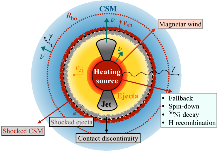
Figure 1: Sketch (not to scale) of the outflow (orange/yellow region) launched by the collapsing star and powered by a central heating source (red region), moving at velocity $v_{\rm{ej}}$. The heating can be due to fallback material on the BH, spin-down of the magnetar, and/or ⁵⁶Ni decay, and hydrogen recombination. A jetted outflow can be harbored (gray region). The outflow expands and interacts with a dense CSM (blue region), forming a forward shock and a reverse shock. The former propagates outwards and it shocks the CSM (red outermost shell), the latter propagates inwards and it shocks the ejecta (light gray shell). The two shocked regions are separated by a contact discontinuity (black dotted line). The forward shock (moving at velocity $v_{\rm{sh}}$) breaks out from the CSM at the breakout radius ($R_{\rm{bo}}$, dotted red line), where non-thermal production of particles starts. Neutrino production can take place at the forward shock propagating in the CSM and eventually in the magnetar wind and/or in the jet.

The total energy radiated by each heating source over the duration of its activity, $t_{\rm{dur}}$, in a specific waveband $\left[E_{\min},E_{\max}\right]$ is

$$E_{\rm{rad}}=\int_{E_{\rm{min}}}^{E_{\rm{max}}}dE_{\gamma}\ E_{\gamma}n_{\gamma}(E_{\gamma})\;,$$ (4)

where $n_{\gamma}$ is the photon distribution resulting from the heating process under consideration. Note that we refer to the total energy radiated after photons diffuse through the ejecta mass. Throughout the paper, we consider the following wavebands:

• Radio: $[E_{\rm{min}}^{\rm{Radio}},E_{\max}^{\rm{Radio}}]=[4\times 10^{-15},4\times 10^{-13}]$ GeV =[$1,100$] GHz;

• Infrared (IR): $[E_{\rm{min}}^{\rm{IR}},E_{\max}^{\rm{IR}}]=[4\times 10^{-13},1.7\times 10^{-9}]$ GeV = [$0.75,300$] $\mu$m;

• Optical: $[E_{\rm{min}}^{\rm{Opt}},E_{\max}^{\rm{Opt}}]=[1.7\times 10^{-9},3.3\times 10^{-9}]$ GeV = [$320,750$] nm;

• Ultraviolet (UV): $[E_{\rm{min}}^{\rm{UV}},E_{\max}^{\rm{UV}}]=[3.3\times 10^{-9},1.2\times 10^{-7}]$ GeV=[$10,320$] nm;

• X-ray: $[E_{\rm{min}}^{\rm{X-ray}},E_{\max}^{\rm{X-ray}}]=[3\times 10^{-7},200\times 10^{-6}]$ GeV= [$0.3,200$] keV;

• Gamma-ray: $[E_{\rm{min}}^{\gamma-\rm{ray}},E_{\max}^{\gamma-\rm{ray}}]=[200\times 10^{-6},10^{3}]$ GeV.

Following Ref. (Villar et al., 2017), we assume that radiation quickly thermalizes and relaxes to a black-body distribution

$$n^{\rm{BB}}_{\gamma}(E_{\gamma})=\int_{0}^{t_{\rm dur}}dtA_{\gamma}(t)\frac{E_{\gamma}^{2}}{e^{E_{\gamma}/k_{B}T_{\gamma}^{\rm{BB}}(t)-1}}\;,$$ (5)

with $k_{B}$ being the Boltzmann constant, $A_{\gamma}(t)=L(t)/\left[\int_{0}^{\infty}dE_{\gamma}E_{\gamma}n_{\gamma}^{\rm{BB}}(E_{\gamma},t)\right]$ the normalization constant and $L$ the emitted luminosity given by Eq. II.1, which depends on the type of heating source.

The blackbody temperature is

$$T_{\gamma}^{\rm{BB}}(t)\simeq\left[\frac{L(t)}{4\pi\sigma_{\rm{SB}}R_{\rm{ph}}(t)^{2}}\right]^{1/4}\;,$$ (6)

where $\sigma_{SB}$ is the Stefan-Boltzmann constant and $R_{\rm{ph}}\simeq R_{\rm{ej}}$ is the photospheric radius in our approximation. Care should be taken for the photon spectrum resulting from CSM interactions; see Sec. II.2.6.

The black-body assumption holds as long as the outflow is optically thick. Since the bulk of energy is emitted near the lightcurve peak with temperature $\simeq T^{\rm{BB}}_{\gamma}$, this is a fair approximation. Note that the total radiated energy in Eq. 4 is calculated in the reference frame of the star, without considering redshift corrections. For a source at redshift $z$, the observed energy is $E_{\rm{obs}}=E_{\rm{rad}}/(1+z)$.

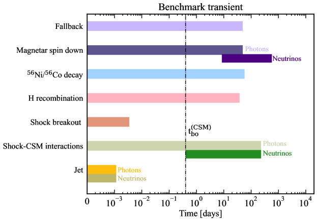
Figure 2: Duration of the bolometric lightcurve powered by different heating processes (Eq. II.1). From top to bottom the observed luminosity is powered by: fallback of material onto a BH, magnetar spin down, ⁵⁶Ni and ⁵⁶Co decay, hydrogen recombination, shock breakout from the progenitor star, CSM interactions in the optically thick and thin regimes, and jet. The vertical line marks the time of breakout from the dense CSM shell (Eq. 19). The time intervals over which neutrino production occurs are displayed for the magnetar scenario, CSM interactions, and the jet.

Table 1: Characteristic parameters for our benchmark transient. Each parameter is defined in the main text for the corresponding heating source. We consider a red supergiant progenitor. These parameters are meant to represent individual heating processes; only a subset of them is expected to be at play for a specific transient source class.

Parameter	Symbol	Value
Ejecta energy	$E_{k,\rm{ej}}$	$10^{51}$ erg
Ejecta mass	$M_{\rm{ej}}$	$M_{\odot}$
Fallback time	$t_{\rm fb}$	$10^{7}$ s
Fallback mass	$M_{\rm fb}$	$10^{-2}M_{\odot}$
Jet efficiency	$\epsilon_{j}$	$10^{-2}$
Density contributing to $M_{\rm{fb}}$	$\bar{\rho}$	$10^{-7}$ cm-3
Spin-down period	$P_{\rm{spin}}$	$10$ ms
Magnetar magnetic field	$B$	$10^{14}$ G
Fraction of ejecta mass in 56Ni	$f_{\rm{Ni}}$	$0.1$
Progenitor radius	$R_{\star}$	$500\ R_{\odot}$
Progenitor mass	$M_{\star}$	$15\ M_{\odot}$
Mass-loss rate	$M_{w}$	$5\times 10^{-3}\;M_{\odot}$ yr-1
Wind velocity	$v_{w}$	$100$ km s-1
CSM radius	$R_{\rm{CSM}}$	$2\times 20^{16}$ cm
Jet isotropic energy	$E_{\rm{iso},j}$	$3.7\times 10^{54}$ erg
Jet lifetime	$t_{j}$	100 s
Jet Lorentz factor	$\Gamma$	$300$
Jet opening angle	$\theta_{j}$	$3^{\circ}$

II.2.1 Fallback

When a massive star undergoes gravitational collapse its core collapses into a Kerr BH (MacFadyen and Woosley, 1999), as predicted by the collapsar model. Due to fast rotation, the outer layers of the collapsing star carry too much angular momentum to fall freely into the last stable orbit. Thus, an accretion disk forms, from which both gravitational and rotational energy can be extracted. Energy may also be released through neutrino cooling (Chen and Beloborodov, 2007).

Besides the unbound mass ejected during the collapse, a comparable mass (e.g., from tidal tails) could remain bound to the central compact object and fallback onto it. The rate at which mass falls back onto the BH is (Lee and Ramirez-Ruiz, 2006; Metzger et al., 2018, 2008; Metzger, 2020; Lopez-Camara et al., 2009):

$$\dot{M}_{\rm{fb}}(t)=\frac{2}{3}\frac{M_{\rm{fb}}}{t_{\rm{fb}}}\frac{1}{\left(1+\frac{t}{t_{\rm{fb}}}\right)^{{5}/{3}}}\;,$$ (7)

where $M_{\rm{fb}}$ is the total accreted mass, $t_{\rm{fb}}=\left(3\pi/32G\bar{\rho}\right)^{1/2}$ is the free-fall time scale (Kippenhahn et al., 2020), $G$ is the gravitational constant, $\bar{\rho}$ is the mean density of the collapsing layer contributing to $M_{\rm{fb}}$. The injected luminosity from this heating process is (Metzger, 2020)

$$L_{\rm{inj}}^{\rm{fb}}(t)=\epsilon_{j}\dot{M}_{\rm{fb}}c^{2}\;,$$ (8)

where $\epsilon_{j}$ is a constant factor representing the fraction of accreted energy which is used to power the disk wind (or jetted outflow), namely its efficiency. The heating of the spherical ejecta occurs either because of a jet which becomes unstable and looses power (Bromberg and Tchekhovskoy, 2016) or a mildly-relativistic wind which is launched by the inner accretion disk and collides with the more massive outflow emitted at the explosion (Dexter and Kasen, 2013). In both cases, the energy available to heat the collapsar outflow is given by Eq. 8; see also the discussion in Ref. (Metzger, 2020).

For a red supergiant progenitor (Table 1), the collapsing layer has mean density $\bar{\rho}\simeq 10^{-7}$ g cm^-3, corresponding to the fallback time $t_{\rm fb}\simeq 10^{7}$ s (Metzger et al., 2018). The total mass accreted in this case is $M_{\rm fb}\simeq 10^{-2}M_{\odot}$ (Chevalier, 1989), resulting in a fallback rate $M_{\rm fb}/t_{\rm fb}\simeq 10^{-9}M_{\odot}$ s^-1. Figure 3 (top left panel) shows the energy radiated across the electromagnetic wavebands (Eq. 4) through fallback of matter on the BH, relative to the kinetic energy of the ejecta $E_{k,\rm{ej}}$. For our benchmark transient, the bulk of radiation powered by fallback onto the BH is emitted in the infrared-optical-ultraviolet (UVOIR) band due to the opacity of the outflow. X-rays may become observable at later times, yet we do not consider this signal in our treatment as it would become relevant at larger times than the ones considered in this work; see (Dexter and Kasen, 2013) for details.

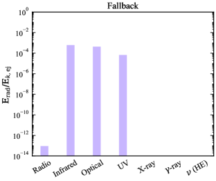
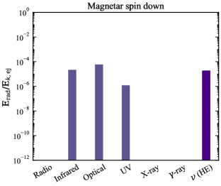
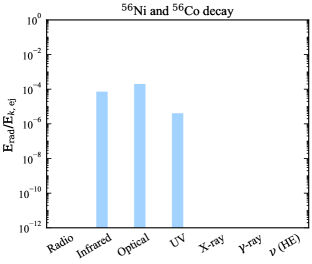
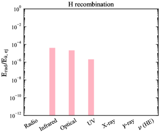
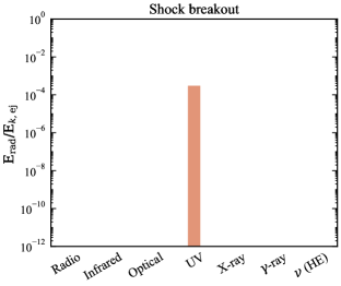
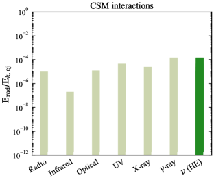
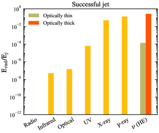
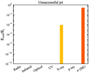
Figure 3: Ratio between the energy radiated across electromagnetic wavebands as well as neutrinos and the kinetic energy of the ejecta (or the energy of the jet for the bottom panels). The results are shown for our benchmark transient (see Table 1). The color code is the same as in Fig. 2 for each heating process. Heating from fallback material on the BH, magnetar spin down, ⁵⁶Ni, and ⁵⁶Co decay and hydrogen recombination lead to emission of radiation in the UVOIR band. The shock breakout produces a flash of light in the UV band. CSM interactions in the optically thin regime mostly radiate in the radio and X-ray bands, with a substantial energy fraction released in gamma-rays and neutrinos. A successful jet radiates in the X-ray and gamma-ray bands, whereas the only electromagnetic signature of unsuccessful jets is the flash of light from the shock breakout emitted in the X-ray/gamma-ray band, depending on the outflow and progenitor properties. The jet radiates energy in neutrinos both in the optically thin and thick regimes, the former component only existing for successful jets.

II.2.2 Magnetar spin down

Assuming a dipole configuration for the magnetic field, the injected luminosity from the spin down of the compact object is

$$L_{\rm{inj}}^{\rm{sd}}(t)=\frac{\epsilon_{\rm{sd}}E_{\rm{sd}}}{t_{\rm{sd}}\left(1+\frac{t}{t_{\rm{sd}}}\right)^{2}}\;,$$ (9)

where $E_{\rm{sd}}=I\Omega^{2}/2$ is the initial rotational energy of the magnetar, which depends on the moment of inertia ($I$) and angular velocity of the neutron star ($\Omega$). The spin-down timescale $t_{\rm{sd}}$ is related to the neutron star magnetic field $B_{14}=B/(10^{14}G)$ and the spin period $P_{\rm{spin}}=2\pi/\Omega\simeq 10~{}[E_{\rm{sd}}/(2\times 10^{50}\;\rm{erg})]^{-0.5}$ ms through (Ostriker and Gunn, 1969)

$$t_{\rm{sd}}=4\times 10^{7}\frac{P_{\rm{spin,10}}^{2}}{B_{14}^{2}}\;\rm{s}\;.$$ (10)

We consider the spin-down injection efficiency to be $\epsilon_{\rm{sd}}=10\%$, relying on observations of the Crab Nebula (Kasen and Bildsten, 2010). Furthermore, we carry out our calculations for a neutron star with $I=10^{45}$ g cm^-2 g cm^-2 (Lattimer and Schutz, 2005).

Figure 3 (top right panel) shows the energy radiated (Eq. 4) through the magnetar spin down. The bulk of radiation powered by the spin down of the magnetar is emitted in the UVOIR band. Note that, during the the time interval that we consider, the outflow is optically thick, hence the non-thermal X-rays produced by the compact object are reprocessed in the optical/UV bands Fang and Metzger (2017).

II.2.3 Radioactive decay of nickel and cobalt

Diffusion of radioactive energy produced by newly sinthetized ⁵⁶Ni and subsequently ⁵⁶Co was investigated in Refs. (Arnett, 1979, 1980; Wheeler et al., 2015) analytically. The injected luminosity in Eq. II.1 can be parametrized as

$$L_{\rm{inj}}^{\rm{Ni}}(t)=M_{\rm{Ni}}\left[\epsilon_{\rm{Co}}e^{-t/\tau_{\rm{Co}}}+(\epsilon_{\rm{Ni}}-\epsilon_{\rm{Co}})e^{-t/\tau_{\rm{Ni}}}\right]\;$$ (11)

where $M_{\rm{Ni}}=f_{\rm{Ni}}M_{\rm{ej}}$ is the fraction of the ejecta mass that goes into ⁵⁶Ni, $\epsilon_{\rm{Ni}}=3.9\times 10^{10}$ erg s^-1 g^-1 ($\epsilon_{\rm{Co}}=6.8\times 10^{9}$ erg s^-1 g^-1) and $\tau_{\rm{Ni}}=8.8$ days ($\tau_{\rm{Co}}=111.3$ days) are the energy generation rates and the decay rates of ⁵⁶Ni (⁵⁶Co), respectively.

Figure 3 (second row, left panel) displays the energy radiated across different wavebands (Eq. 4) through radioactive decay of ⁵⁶Ni and ⁵⁶Co. The bulk of radiation powered by these processes is emitted in the UVOIR band; also in this case, the resulting bulk of radiation depends on the assumption of optically thick ejecta.

II.2.4 Hydrogen recombination

When the collapsing massive star retains its hydrogen layer, the latter can be ionized by the SN shock. Hydrogen recombination takes place as the outflow cools to $\approx 5000$ K, which is the ionization temperature of neutral hydrogen and it has been invoked to explain the plateau observed in the lightcurve of some SNe (Hamuy, 2003; Smartt et al., 2009; Sanders et al., 2015; Rubin et al., 2016). An analytical model for hydrogen recombination was presented in Refs. (Woosley, 1993; Kasen and Woosley, 2009; Sanders et al., 2015; Villar et al., 2017; MacLeod et al., 2017; Kasen and Ramirez-Ruiz, 2010).

The luminosity $L_{p}$ and duration $t_{p}$ of the plateau are (Woosley, 1993)

$$L_{p} = 1.64\ \times 10^{42}\frac{R_{\star,500}^{2/3}E_{k,51}^{5/6}}{M_{\rm{ej},10}^{1/2}}\;\rm{erg}\;\rm{s}^{-1}\;,$$ (12)

$$t_{p} = 99\ \frac{M_{\rm{ej,}10}^{1/2}R_{\star,500}^{1/6}}{E_{k,51}^{1/6}}\;\rm{days}\,,$$ (13)

where $R_{\star,500}=R_{\star}/(500\ R_{\odot})$, $E_{k,51}=E_{k,\rm{ej}}/(10^{51}$ erg) and $M_{\rm{ej},10}=M_{\rm{ej}}/(10\ M_{\odot})$ are the kinetic energy and the mass of the ejecta, respectively, with $R_{\odot}$ and $M_{\odot}$ being the solar radius and mass.

The injected luminosity from hydrogen recombination is (Sanders et al., 2015)

$$L_{\rm{inj}}^{\rm{H}}(t)=\frac{L_{p}}{e^{-(13.1+0.47\ M_{p})t}}\;,$$ (14)

where $M_{p}$ is the peak magnitude, linked to the peak luminosity ($L_{p}$).

The energy radiated across different wavebands through hydrogen recombination is shown in Fig. 3 (second row, right panel). The bulk of radiation powered by hydrogen recombination is emitted in the UVOIR band.

II.2.5 Shock breakout

A flash of light is expected when the forward shock driven by the outflow breaks out from the progenitor star. When the CSM surrounding the collapsing star is very dense, the shock breakout may however take place when the shock crosses the CSM.

The shock breakout theory has been developed in Refs. (Nakar and Sari, 2010, 2012; Waxman and Katz, 2017) for non-relativistic and (mildly-)relativistic shocks. The former is the regime expected for standard core-collapse SNe, while the latter is relevant for engine-driven SNe. The models of Refs. (Nakar and Sari, 2010, 2012) are challenged by observations, as they cannot reproduce the duration and luminosity of the candidate SNe possibly displaying shock breakout, see e.g. Refs. (Soderberg et al., 2008; Alp and Larsson, 2020; Novara et al., 2020). Yet, an advanced shock breakout theory does not exist to date. In the light of these uncertainties, we do not adopt any spectral energy distribution for the shock breakout emission. Rather, we assume that photons with temperature $T_{\rm{bo}}$ are emitted over the time $t_{\rm{bo}}$, with total energy release $E_{\rm{bo}}$. These quantities depend on the stellar progenitor radius ($R_{\star}$) and mass ($M_{\star}$), as well as on the energy of the ejecta. For instance, in the case of a non-relativistic shock breakout from a red supergiant one has (Nakar and Sari, 2010):

$$T_{\rm{bo}} \simeq 25\;\rm{eV}\ M_{\star,15}^{-0.3}\ R_{\star,500}^{-0.65}\ E_{k,\rm{ej},51}^{0.5}\;;$$ (15)

$$t_{\rm{bo}} \simeq 300\;\rm{s}\ M_{\star,15}^{0.21}\ R_{\star,500}^{2.16}\ E_{k,\rm{ej},51}^{-0.79}\;;$$ (16)

$$E_{\rm{bo}} \simeq 9\times 10^{47}\;\rm{erg}\ M_{\star,15}^{-0.43}\ R_{\star,500}^{1.74}\ E_{k,\rm{ej},51}^{0.56}\;,$$ (17)

where $M_{\star,15}=M_{\star}/(15M_{\odot})$, $R_{\star,500}=R_{\star}/(500R_{\odot})$ and $E_{k,\rm{ej},51}=E_{k,\rm{ej}}/(10^{51}\;\rm{erg})$. The analytical expressions of these parameters for other stellar progenitors are listed in Appendix A of Ref. (Nakar and Sari, 2010) for non-relativistic shocks and Eq. 29 of Ref. (Nakar and Sari, 2012) for (mildly-)relativistic shocks. Note that the flash of light produced at the breakout from the stellar surface should be followed by the cooling of the envelope (Nakar and Sari, 2010, 2012). However, we neglect this contribution, as it is not correlated with neutrino emission and thus not of relevance for the purposes of this work.

Figure 3 (third row, left panel) shows the energy radiated across different wavebands $E_{\rm{rad}}$ (Eq. 4) through shock breakout. For our benchmark transient, the non-relativistic shock breakout produces a burst of photons in the UV band.

II.2.6 Interaction with the circumstellar medium

Towards the end of their life, massive stars can undergo eruptive episodes, polluting the surrounding environment. As a consequence, the collapsing star could have a dense CSM shell. We assume that the CSM density follows a wind profile

$$\rho_{\rm{CSM}}(R)=\frac{\dot{M}_{w}}{4\pi R^{2}v_{w}f_{\Omega}}\;$$ (18)

where $\dot{M}_{w}$ is the mass-loss rate of the star, $v_{w}$ is the wind speed, and $f_{\Omega}$ is the fraction of the solid angle with dense CSM. Unless otherwise specified, we assume a spherically symmetric CSM ($f_{\Omega}=1$), extended up to the external radius $R_{\rm{CSM}}$, where its density is assumed to drop sharply. As the outflow expands in the CSM, two shocks form: the forward shock, propagating outward and shocking the CSM material, and the reverse shock propagating backward and shocking the ejecta (in mass coordinates) (Chevalier and Fransson, 2017). The forward shock is the main site of dissipation of kinetic energy, whereas the contribution of the reverse shock is expected to be subleading at the epochs considered in this work and for non-relativistic shocks Ellison et al. (2007); Patnaude and Fesen (2009); Schure et al. (2010); Suzuki et al. (2020); Slane et al. (2014); Sato et al. (2018). The slow deceleration of the forward shock during its interaction with the CSM is not relevant to our purposes, as it would not affect substantially the neutrino emission; we assume that the interaction with the CSM has a total duration $t_{\rm{dur}}\simeq R_{\rm{CSM}}/v_{\rm{sh}}$, where $v_{\rm{sh}}$ is the velocity of the forward shock.

The forward shock breaks out from the CSM at the breakout radius $R_{\rm{bo}}$, defined through the following relation

$$\tau_{\rm{CSM}}(R_{\rm{bo}})=\int_{R_{\rm{bo}}}^{R_{\rm{CSM}}}dR\;\rho_{\rm{CSM}}(R)\kappa_{\rm{CSM}}=\frac{c}{v_{\rm{sh}}}\;,$$ (19)

As the forward shock interacts with the CSM, its kinetic energy is converted into radiation. Within the approximation of constant shock velocity and efficient shock radiation, the injected and emitted luminosity coincide (Ofek et al., 2014):

$$L_{\rm{inj}}^{\rm{CSM}}\equiv L(t)=2\pi\epsilon_{\rm{eff}}\rho_{\rm CSM}(t)R_{\rm{sh}}(t)^{2}v_{\rm{sh}}^{3},$$ (20)

where $\epsilon_{\rm eff}$ is the efficiency conversion factor of kinetic energy into radiation, $R_{\rm{sh}}=v_{\rm{sh}}t$ is the shock radius, and $\rho_{\rm{CSM}}$ is given by Eq. 18 and evaluated at $R_{\rm{sh}}(t)$. As the bulk of radiation from CSM interactions is radiated around $R_{\rm{bo}}$ (Pitik et al., 2023), we assume that the total luminosity emitted in the range $R_{0}\leq R\leq R_{\rm{bo}}$ is $L\simeq L_{\rm{bo}}$.

Within our simple framework, the effective temperature of the black-body distribution emerging at $R_{\rm{bo}}$ is (Chevalier and Irwin, 2011; Ofek et al., 2014):

$$T_{\gamma}^{\rm{BB}}=\left(\frac{18}{7a}\rho_{\rm{CSM}}(R_{\rm{bo}})v_{\rm{sh}}^{2}\right)^{1/4}\;.$$ (21)

Once the forward shock breaks out from the dense CSM, namely when Eq. 19 is fulfilled, it becomes collisionless. In this regime, photons are mainly produced through bremsstrahlung and emitted in the X-ray band for $v_{\rm{sh}}\gtrsim 10^{4}$ km s^-1 (Margalit et al., 2022). The total emitted luminosity produced by the forward shock for $R_{\rm{bo}}\leq R\leq R_{\rm{CSM}}$ is given by (Margalit et al., 2022; Fang et al., 2020)

$$L^{\rm{brem}}(R_{\rm{CSM}})=\min\left(0.3\frac{t_{\rm{dyn}}}{t_{\rm{ff}}},1\right)L_{\rm{sh}}\;,$$ (22)

where $t_{\rm{dyn}}$ and $t_{\rm{ff}}$ are the dynamical and free-free electron cooling times defined as in Appendix B. The shock kinetic power $L_{\rm{sh}}$ is also defined in Appendix B. Note that Eq. 22 is estimated at the edge of the CSM shell ($R_{\rm{CSM}}$).

After shock breakout from the CSM, the radiation due to CSM interactions no longer relaxes to a black-body distribution, hence the non-thermal photon spectrum is

$$n^{\rm{brem}}_{\gamma}(E_{\gamma})=L^{\rm{brem}}\frac{E_{\gamma}}{k_{B}T_{e}}e^{-E_{\gamma}/k_{B}T_{e}}\;,$$ (23)

where $L^{\rm{brem}}$ is the total emitted luminosity given by Eq. 22 and $T_{e}$ is the post-shock temperature of electrons, defined in Appendix B.

In the optically thin region of the CSM, particle acceleration leads to production of relativistic electrons. This case is particularly relevant when shocks are not radiative. As the forward shock expands in the CSM, it converts the kinetic energy of the blastwave into internal energy. The internal energy density is

$$u_{\rm{int}}(R)=\frac{9}{8}v_{\rm{sh}}^{2}\ \rho_{\rm{CSM}}\ ,$$ (24)

where $\rho_{\rm{CSM}}$ is given by Eq. 18. A fraction $\epsilon_{B}$ of the internal energy density is stored in the post shock magnetic field $B_{\rm{CSM}}=\sqrt{8\pi\epsilon_{B}u_{\rm{int}}}$.

A fraction $\epsilon_{e}$ of Eq. 24 is given to accelerated electrons. The latter mostly cool through synchrotron radiation (Chevalier, 1998), whose spectrum for the non-relativistic and mildly-relativistic blastwave is provided in Ref. (Margalit et al., 2022).

In Fig. 3 (third row, right panel) we show the total energy radiated through CSM interactions. We also display the relative energy emitted in gamma-rays (see Sec. IV). The bulk of energy is radiated in the UVOIR band, whereas bremsstrahlung and synchrotron processes radiate energy mostly in the radio and X-ray bands.

II.2.7 Multiple heating sources

If more than one source contributes to heat the outflow as it expands, the total radiated luminosity is given by the sum of all contributions: $L^{\rm{tot}}=\sum_{i}L^{i}(t)$, where $L^{i}$ corresponds to the luminosity radiated from the $i$-th heating source.

If the outflow propagates in a dense CSM, then the radiation produced by other heating sources (e.g., ⁵⁶Ni decay) has to propagate through the total mass $M_{\rm{tot}}=M_{\rm{ej}}+M_{\rm{CSM,th}}$, where $M_{\rm{CSM,th}}=\int_{R_{\star}}^{R_{\rm{bo}}}dR4\pi R^{2}\rho_{\rm{CSM}}(R)$ is the mass of the optically thick CSM.

III Modeling of the electromagnetic emission: jetted relativistic outflows

In this section, we focus on the modeling of the electromagnetic emission in jetted relativistic outflows, which differs from the treatment outlined in Sec. II for the non-relativistic outflows. A bipolar jet may be harbored in the collapsing star and launched a few ms after the collapse. Given the jet luminosity ${L}_{j}$ (assumed to be constant) and lifetime ${t}_{j}$, its injected energy is ${E}_{j}={L}_{j}{t}_{j}$. The jet dynamics only depends on the jet isotropic equivalent energy ${E}_{\rm{iso},j}={E}_{j}/({\theta}_{j}^{2}/4)$ and Lorentz factor $\Gamma$ (Piran, 1999; Kumar et al., 2008), where $\theta_{j}$ is the jet opening angle. We parameterize the energy budget of the jet in terms of its energy $E_{j}$ (Kaneko et al., 2006), rather than $E_{k,\rm{ej}}$ as we have considered for the non-relativistic outflows (see Fig. 3). Furthermore, our results refer to a jet observed on-axis (for a discussion on jets observed off-axis see, e.g., Ref. Ramirez-Ruiz et al. (2005a)).

Short living engines or progenitor stars which retain the hydrogen envelope, such as partially stripped SNe, are likely to produce unsuccessful jets (Lee and Ramirez-Ruiz, 2006; Izzard et al., 2004; Nakar, 2015; Gilkis and Arcavi, 2022; Sobacchi et al., 2017). In this case, the jetted outflow does not breakout from the stellar mantle or it is choked. If the jet is instead powered for sufficiently long time and is energetic enough, it breaks out from the star and produces a GRB.

III.1 Successful jets

The mechanism responsible for energy dissipation and shaping the observed non-thermal emission is still under debate, with particle acceleration possibly due to internal shocks Rees and Meszaros (1994); Daigne and Mochkovitch (1998); Kobayashi et al. (1997) or magnetic reconnection (Zhang and Yan, 2011; Drenkhahn, 2002; Drenkhahn and Spruit, 2002; Giannios, 2008). In both cases, the observed electromagnetic signal may originate both in the optically thick and thin regions of the jet. Following Ref. (Pitik et al., 2021) , Fig. 3 (bottom left panel) shows the total energy radiated by a successful jet across the electromagnetic wavebands, assuming $t_{\rm{dur}}=100$ s (Tarnopolski, 2015; Gehrels et al., 2009). We show the largest energy radiated among the GRB models considered in Ref. (Pitik et al., 2021), in order to obtain an upper limit for the energy budget. Note that the relativistic component of the outflow moves with constant Lorentz factor $\Gamma$, hence the observed energy is $E_{\rm{obs}}=E_{\rm{rad}}\Gamma/(1+z)$.

We do not consider the deceleration phase of the relativistic jetted component of the outflow. This is motivated by the fact that the neutrino emission during the afterglow is negligible with respect to the prompt one Guarini et al. (2022b).

III.2 Unsuccessful jets

As the jet propagates through the stellar envelope, it inflates a high pressure region of shocked jet and stellar material, the cocoon (Bromberg et al., 2011; Ramirez-Ruiz et al., 2002; Lazzati and Begelman, 2005; Zhang et al., 2003). The jet dynamics is highly non-linear due to the mixing with the cocoon, which slows down the jet while increasing its baryon density (Gottlieb et al., 2022a) (see Ref. (Bromberg et al., 2011) for the analytical modeling of the propagation of a relativistic jet in the stellar mantle). Independently on the fate of the jet, the cocoon always breaks out from the star (Bromberg et al., 2011; Lazzati and Begelman, 2005).

If the jet is smothered within the stellar mantle, the only observable electromagnetic counterpart would be the shock breakout of the cocoon from the collapsing star. The breakout is expected to occur with mildly-relativistic velocities, with signatures of asymmetries in the outflow (Gottlieb et al., 2020; Maeda et al., 2023). The fraction of energy radiated from an unsuccessful jet is shown in Fig. 3 (bottom right panel), for the parameters used in Ref. (Guarini et al., 2023).

IV Neutrino emission

In this section, we summarize the processes leading to neutrino production, namely photo-hadronic ($p\gamma$) and hadronic ($pp$) interactions. Furthermore, we outline the methods adopted to calculate the neutrino signal.

IV.1 Proton spectral energy distribution

The regions of the outflow where protons can be co-accelerated with electrons are the magnetar wind, the forward shock resulting from CSM interactions and the jet. We now introduce the resulting spectral energy distributions of protons.

Magnetar wind.

The injected proton energy distribution is [in units of GeV^-1 cm^-3] (Fang and Metzger, 2017)

$${n}_{{p}}({E}_{p})\equiv\frac{{\rm{d}}^{2}{N}_{{p}}}{{\rm{d}}{E}_{{p}}{\rm{d}}{V}}=A_{p}E^{-1}_{p}\ ,$$ (25)

where the normalization constant is $A_{p}=1.08\times 10^{-5}B_{14}^{-1}t_{5.5}^{-3}M_{\rm{ej},-2}^{3/2}P_{\rm{spin},-3}^{3}$, with $t_{5.5}=t/10^{5.5}$ s, and the other quantities are defined as in Sec. II.2. Note that the spectrum of protons accelerated in the magnetar wind is expected to be hard [$n_{p}(E_{p})\propto E^{-1}_{p}$].

CSM interactions.

Protons can be accelerated at the forward shock as the SN ejecta cross the CSM. Efficient acceleration starts at $R\simeq R_{\rm{bo}}$ (Murase et al., 2011; Petropoulou et al., 2017; Pitik et al., 2021; Katz et al., 2011; Sarmah et al., 2022) and it proceeds over a wide range of radii, up to the outer radius $R_{\rm{out}}=\min\left[R_{\rm{CSM}},R_{\rm{dec}}\right]$. Here, $R_{\rm{dec}}=M_{\rm{ej}}v_{w}/\dot{M}_{w}$ is the deceleration radius, corresponding to the distance from the center of explosion where the outflow has swept-up a CSM mass comparable to $M_{\rm{ej}}$.

The injected proton energy distribution at the forward shock is [in units of GeV cm^-3]:

$${n}_{{p}}({E}_{p})\equiv\frac{{\rm{d}}^{2}{N}_{{p}}}{{\rm{d}}{E}_{{p}}{\rm{d}}{V}}={A}_{p}{E}_{{p}}^{-k_{p}}\Theta({E}_{{p}}-{E}_{p,\rm{min}})\Theta({E}_{p,\rm{max}}-{E}_{\rm{p}})\ ,$$ (26)

where $k_{p}=2$ is the proton index for non-relativistic collisionless shocks (Matthews et al., 2020). The minimum proton energy for non-relativistic shocks is ${E}_{p,\rm{min}}=m_{p}c^{2}$ (for mildly-relativistic shocks, the minimum proton energy is ${E}_{p,\rm{min}}=\Gamma_{\rm{sh}}m_{p}c^{2}$, where $\Gamma_{\rm{sh}}=1/\sqrt{1-(v_{\rm{sh}}/c)^{2}}$ is the shock Lorentz factor; since for mildly-relativistic shocks $\Gamma_{\rm{sh}}\lesssim 2$, the correction to the minimum proton energy does not affect our results for the neutrino signal substantially), while the maximum energy ${E}_{p,\rm{max}}$ is obtained by the condition ${t}_{p,\rm{acc}}^{-1}={t}^{-1}_{p,\rm{cool}}$, where ${t}^{-1}_{p,\rm{acc}}$ is the proton acceleration rate and ${t}^{-1}_{p,\rm{cool}}$ is the proton total cooling rate; see Appendix A for the proton cooling rates.

The normalization constant is ${A}_{p}={9\epsilon_{{p}}n_{{p,\rm{CSM}}}}(R)m_{p}c^{2}/[{8{\rm{ln}}({E}_{p,\rm{max}}/{E}_{p,\rm{min}})}]({v_{\rm{sh}}}/c)^{2}$. Here, $\epsilon_{p}$ is the fraction of the blastwave internal energy expressed by Eq. 24 which is stored into accelerated protons. Finally, $n_{p,\rm{CSM}}=\rho_{\rm{CSM}}/m_{p}$ is the CSM proton number density.

Jetted outflows.

Protons accelerated in the jet follow a power-law spectrum Sironi et al. (2013). The proton distribution in the comoving frame of the jet (we denote quantities in this frame as primed: $X^{\prime}$) reads [in units of GeV cm^-3]

$$n^{\prime}_{p}(E^{\prime}_{p})=\frac{{\rm{d}}^{2}N^{\prime}_{\rm{p}}}{{\rm{d}}E^{\prime}_{\rm{p}}{\rm{d}}V^{\prime}} = A^{\prime}_{p}E^{{}^{\prime}-k_{p}}_{p}\exp\left[-\left(\frac{E^{\prime}_{p}}{E^{\prime}_{p,\rm{max}}}\right)^{\alpha_{p}}\right]$$ (27)

$$\times \Theta(E^{\prime}_{p}-E^{\prime}_{p,\rm{min}})\ ,$$

where $\alpha_{p}$ mimics an exponential cutoff (Malkov and Drury, 2001) and $\Theta$ is the Heaviside function. The minimum energy of accelerated protons is $E^{\prime}_{p,\min}=m_{p}c^{2}$, while their maximum energy is obtained equating the proton acceleration rate with the proton cooling rate, namely $t^{\prime-1}_{p,\rm{acc}}=t^{\prime-1}_{p,\rm{cool}}$; see Appendix A for the proton cooling rates in the jet. $A^{\prime}_{p}=\epsilon_{j,d}\epsilon_{j,p}E^{\prime}_{\rm{iso},j}/(4\pi R_{j}^{2}ct^{\prime}_{j})$ is the normalization constant, where $\epsilon_{j,p}$ is the fraction of the dissipated isotropic energy of the jet $\epsilon_{j,d}E^{\prime}_{\rm{iso}}$ which is stored in accelerated electrons; $R_{j}$ is the position along the jet where proton acceleration takes place, while $t^{\prime}_{j}={t}_{j}\Gamma$ is the comoving jet lifetime.

The microphysical parameters $\epsilon_{j,d}$ and $\epsilon_{j,p}$ depend on the process assumed to be responsible for energy dissipation along the jet. The spectral index is $k_{p}=2.2$, if acceleration occurs at relativistic collisionless internal shocks or sub-shocks (Sironi et al., 2013; Beloborodov, 2017), while it depends on the magnetization of the jet if protons are accelerated through magnetic reconnection (Werner et al., 2018).

IV.2 Neutrino production channels

Proton-photon ($p\gamma$) interactions.

Electrons co-accelerated with protons cool producing a photon distribution which serves as a target for accelerated protons. Neutrinos are mainly produced through the $\Delta^{+}$ resonance (Kelner and Aharonian, 2008; Huemmer et al., 2010):

$$p+\gamma\longrightarrow\Delta^{+}\longrightarrow\left\{\begin{array}[]{@{}l@{}}n+\pi^{+}\;\;\;\;\;\;\;1/3\;\rm{\;of\;all\;cases}\\ p+\pi^{0}\;\;\;\;\;\;\;\;2/3\;\rm{\;of\;all\;cases}\ .\end{array}\right.$$ (28)

Subsequently, neutral pions decay into gamma-rays $\pi^{0}\longrightarrow 2\gamma$, while charged pions decay producing neutrinos $\pi^{+}\longrightarrow\mu^{+}+\nu_{\mu}\longrightarrow\bar{\nu}_{\mu}+\nu_{e}+e^{+}$. Unless otherwise specified, we do not distinguish between neutrinos and antineutrinos in the following.

Proton-proton ($pp$) interactions.

Accelerated protons can interact with a target of non-relativistic protons, producing neutral and charged pions (Kelner et al., 2006). Subsequently, pions decay as detailed above for $p\gamma$ interactions. Throughout the paper, we consider the energy radiated in gamma-rays both through the electromagnetic processes discussed in Sec. II and through $pp$ interactions.

IV.3 Expected neutrino emission

Both $p\gamma$ and $pp$ interactions can take place in the magnetar wind, at the external shock driven by the outflow in the CSM and in the jet. The duration of the expected neutrino signals in the wind of a central magnetar and at CSM interactions is summarized in Fig. 2 for our benchmark transient, whose parameters are listed in Table 1. Along the jet, neutrino production takes place throughout the whole jet lifetime $t_{j}$.

Both neutrinos and photons at CSM interactions are produced through the dissipation of kinetic energy of the blastwave as the forward shock expands within the optically thin CSM. Consequently, the duration of the electromagnetic and neutrino signals in Fig. 2 is similar. On the contrary, neutrino production in the magnetar wind starts when photopion production becomes efficient and it ceases when pion production freezes out (Fang and Metzger, 2017); these times are defined in Appendix A. As the processes producing photons and neutrinos in the magnetar wind are not correlated, their duration in Fig. 2 is different.

Magnetar wind.

Protons accelerated in the wind of the magnetar can undergo both $p\gamma$ and $pp$ interactions. The injected proton energy distribution is given by Eq. 25, while thermal optical photons and non-thermal X-ray photons produced in the wind nebula serve as targets for $p\gamma$ interactions.

We calculate the total energy emitted in neutrinos in the magnetar wind following Ref. (Fang and Metzger, 2017):

$${E}^{\nu}_{\rm{tot}} \simeq 1.7\times 10^{41}\eta_{-1}^{2/3}B_{14}^{-4/3}M_{\rm{ej},-2}^{-1/4}P_{\rm{spin},-3}^{-1/2}$$

$$\times\;\epsilon_{\rm{mag},-2}^{-1/6}f^{p}_{\rm{sup}}f^{\pi}_{\rm{sup}}f^{\mu}_{\rm{sup}}\;\rm{erg}\;,$$

where $\eta_{-1}=\eta/10^{-1}$ is the acceleration efficiency in the magnetar wind nebula normalized to its nominal value, $\epsilon_{\rm{mag},-2}=\epsilon_{\rm{mag}}/10^{-2}$ is the nebula magnetization parameter, whose nominal value is motivated by observations of the Crab Nebula (Kennel and Coroniti, 1984). Finally, $f^{p}_{\rm{sup}}$ is the suppression factor for pion creation, while $f^{\pi}_{\rm{sup}}$ and $f^{\mu}_{\rm{sup}}$ are the suppression factors for neutrino creation from $\pi^{\pm}$ and $\mu^{\pm}$ decays, respectively (see Appendix B). The fraction of the ejecta kinetic energy emitted in neutrinos in the magnetar wind is shown in Fig. 3 (top right panel) for our benchmark transient.

CSM interactions.

Accelerated protons follow the input energy distribution in Eq. 26 and can interact with the photon spectrum produced at the forward shock. Furthermore, accelerated protons undergo $pp$ interactions with the non-relativistic CSM protons.

In most cases, $p\gamma$ interactions at the forward shock are subleading for non-relativistic and mildly-relativistic shocks Pitik et al. (2022); Guarini et al. (2022b, a); Murase et al. (2011); Petropoulou et al. (2017); Sarmah et al. (2022). This result also holds when the shocks are radiative, as the energy threshold for $p\gamma$ interactions can be reached only when the CSM covers a small fraction of the solid angle ($f_{\Omega}\ll 1$), which is not the case for SNe (Fang et al., 2020; Brethauer et al., 2022). Therefore, we only consider $pp$ interactions as a viable neutrino production channel at the forward shock. We calculate the total energy emitted in neutrinos through $pp$ interactions following Refs. (Kelner et al., 2006; Petropoulou et al., 2017). The fraction of the ejecta kinetic energy radiated in neutrinos from CSM interactions for our benchmark transient is shown in Fig. 3 (third row, right panel).

Jetted outflows.

In a magnetized jet, neutrino production begins in the optically thick part of the outflow (Gottlieb and Globus, 2021; Guarini et al., 2023). Hereafter we rely on the results of Ref. (Guarini et al., 2023) for the expected neutrino signal. In particular, we consider the case with initial jet magnetization $\sigma_{0}=200$ of Ref. (Guarini et al., 2023).

In the absence of jet magnetization, neutrino production below the jet photosphere may take place only if the jet is smothered in an extended envelope surrounding the progenitor core. We refer the interested reader to Refs. (Senno et al., 2016; Guarini et al., 2022a) for the neutrino signal expected in this scenario, and we explicitly include it in our calculations in Sec. V. However, in Fig. 3 (bottom right panel) we only show the case of a jet smothered in a Wolf-Rayet progenitor star.

In the optically thin region of the jet, the input proton distribution is given by Eq. 27. The non-thermal photon distribution that serves as target for $p\gamma$ interactions depends on the mechanism assumed for energy dissipation. We rely on Ref. (Pitik et al., 2022) and take the maximum energy radiated in neutrinos across the different GRB models considered in the aforementioned reference. In the optically thin part of the jet, the baryon density is not large enough for $pp$ interactions to be efficient Pitik et al. (2022). Therefore, we only consider $p\gamma$ interactions as the viable channel for neutrino production.

In the bottom left panel of Fig. 3 we show the energy radiated by a successful jet in neutrinos both in the optically thick and thin regimes. However, we warn the reader that the results for the optically thick regime outlined in Ref. (Guarini et al., 2023) are obtained for a jet with isotropic luminosity larger than the one assumed for the optically thin component in Ref. (Pitik et al., 2021); the comparison in the bottom left panel of Fig. 3 is intended to be representative.

Table 2: Characteristic parameters for each class of transients originating from the collapse of massive stars considered throughout this work.

Parameter	SNe Ib/c	SNe Ib/c BL with jet	SNe IIP	SNe IIn	SLSNe	LFBOTs
$E_{k,\rm{ej}}$ [erg]	$10^{51}$	$10^{52}$	$10^{51}$	$10^{51}$	$10^{52}$	$10^{52}$
$M_{\rm{ej}}$ [M⊙]	1	1	5	2	5	$10^{-1}$
$M_{\rm{fb}}/t_{\rm{fb}}$ [M⊙ s-1]	N/A	$5\times 10^{-4}$	N/A	N/A	N/A	$1.5\times 10^{-8}$
$\epsilon_{j}$	N/A	0.01	N/A	N/A	N/A	0.01
$\bar{\rho}$ [cm-3]	N/A	100	N/A	N/A	N/A	$10^{-7}$
$P_{\rm{spin}}$ [ms]	N/A	N/A	N/A	N/A	$5$	1
$B$ [G]	N/S	N/A	N/A	N/A	$10^{15}$	$10^{15}$
$f_{\rm{Ni}}$	0.1	0.15	$10^{-3}$	0.01	0.01	0.01
$R_{\star}$ [R⊙]	4	4	500	434	434	434
$M_{w}$ [M⊙ yr-1]	$10^{-5}$	$10^{-5}$	$10^{-3}$	$10^{-2}$	$10^{-2}$	$10^{-3}$
$v_{w}$ [km s-1]	$1000$	$1000$	15	100	100	1000
$\epsilon_{\rm{eff}}$	0.1	0.1	0.1	0.1	0.1	0.1
$\epsilon_{e}$	$10^{-1}$	$10^{-1}$	$10^{-1}$	$10^{-1}$	$10^{-1}$	$10^{-1}$
$\epsilon_{B}$	$10^{-1}$	$10^{-2}$	$10^{-2}$	$10^{-2}$	$10^{-2}$	$10^{-2}$
$\epsilon_{p}$	$10^{-1}$	$10^{-1}$	$10^{-1}$	$10^{-1}$	$10^{-1}$	$10^{-1}$
$E_{\rm{iso},j}$ [erg]	N/A	$3.7\times 10^{54}$	N/A	N/A	N/A	$2.5\times 10^{53}$
$\Gamma$	N/A	$300$	N/A	N/A	N/A	$100$
$\theta_{j}$	N/A	$3^{\circ}$	N/A	N/A	N/A	$6^{\circ}$
$\epsilon_{j,d}$	N/A	0.2	N/A	N/A	N/A	0.2
$\epsilon_{j,p}$	N/A	0.1	N/A	N/A	N/A	0.1

V Transients from collapsing massive stars

In this section, we present the energy radiated through the mechanisms outlined in Sec. II across the electromagnetic wavebands as well as in neutrinos, for the transients originating from collapsing stars: SNe Ib/c as well as SNe Ib/c broad line (BL) and GRBs, SNe IIP, SNe IIn, SLSNe, and LFBOTs. The considered transient categories together with the characteristic parameters adopted for each of the heating processes are listed in Table 2. While a range of parameters should be considered (Villar et al., 2017), we aim to compute ballpark figures for the source energetics to gauge the best multi-messenger detection strategies.

One should also consider neutrinos from the shock breakout from the progenitor star. A calculation of the neutrino signal arising from the breakout of a (quasi) spherical outflow has been attempted in Ref. (Gottlieb and Globus, 2021), which concluded that other dissipation mechanisms taking place within the outflow dominate the time integrated neutrino signal. Furthermore, the photon spectrum emerging from shock breakout is highly uncertain and it is challenging to reproduce observations. In the light of such uncertainties, we neglect neutrinos in the energy budget of shock breakout and leave this task to future work.

V.1 Supernovae of Type Ib/c, Ib/c broad line and gamma-ray bursts

Type Ib/c SNe and GRBs are thought to be linked to massive and compact hydrogen-depleted stars, which experience reduced mass loss ($\dot{M}_{w}\simeq 10^{-7}$–$10^{-4}\;M_{\odot}$yr^-1) (Smith, 2014; Gagliano et al., 2022; Jung et al., 2022). The wind velocities are typically $v_{w}\simeq 10^{3}$ km s^-1 (Margutti et al., 2017). For Type Ib/c SNe, ⁵⁶Ni decay, CSM interactions and shock breakout of a non-relativistic outflow from a Wolf-Rayet star can contribute to heat the outflow.

Figure 4 (top left panel) shows the fraction of energy radiated across different electromagnetic wavebands and in neutrinos for SNe Ib/c. Radioactive decay of ⁵⁶Ni is the most relevant heating source for SNe Ib/c and it radiates the bulk of energy in the UVOIR band, with $E^{\rm{UVOIR}}/E_{k,\rm{ej}}\simeq 10^{-4}$.

The forward shock mediating CSM interactions is the only site of neutrino production for SNe Ib/c, as detailed in Sec. IV. Due to the small mass-loss rates of Wolf-Rayet stars (Ramirez-Ruiz et al., 2005b), this class of SNe is not expected to radiate a bright neutrino signal ($E^{\nu}/E_{k,\rm{ej}}\lesssim 10^{-11}$), consistently with the findings of Ref. (Sarmah et al., 2022). However, about $10\%$ of SNe Ib/c show signs of late time interaction with a dense CSM (Margutti et al., 2017), starting $\gtrsim 1$ year after the explosion [SNe Ib/c late time (LT)]. SNe Ib/c LT can release an amount of energy in neutrinos larger than standard SNe Ib/c. An investigation of the neutrino production due to CSM interactions for this class of SNe can be found in Refs. (Sarmah et al., 2022, 2023).

The number of SNe observed with broad spectral features similar to the ones of SN 1998bw—dubbed SNe Ib/c broad line (BL)—is growing (Berger et al., 2002; Milisavljevic et al., 2015b; Pignata et al., 2011). Many of these SNe are not observationally linked to GRBs Berger et al. (2002), even though their ejecta move with mildly-relativistic velocity ($v_{\rm{ej}}\gtrsim 0.1c$), hinting that the explosion mechanism may be different from the one of standard core-collapse SNe. It has been suggested that the explosion of SNe Ib/c BL is not spherical, but either accompanied by an off-axis GRB Kawabata et al. (2002) or a jet that barely fails to break out from the stellar mantle Margutti et al. (2014). Due to the very high energies, SNe Ib/c BL and GRBs are usually modeled by considering a spinning BH (Woosley, 1993; Kumar et al., 2008; Hayakawa and Maeda, 2018) or a magnetar (Duncan and Thompson, 1992; Mazzali et al., 2006; Metzger et al., 2011) that powers the outflow.

For the class of SNe Ib/c BL, the contribution of fallback material onto the central compact object should be included as an energy source. The fraction of energy radiated across different electromagnetic wavebands and in neutrinos for SNe Ib/c BL is shown in Fig. 4 (top right panel). Fallback of matter on the BH constitutes the most important heating source for SNe Ib/c BL, with $E^{\rm{UVOIR}}/E_{k,\rm{ej}}\simeq 2\times 10^{-4}$. If the central engine is not efficient then radiation is powered by ⁵⁶Ni decay only. Similarly to SNe Ib/c, CSM interactions are not an efficient neutrino production mechanism for SNe Ib/c BL ($E^{\nu}/E_{k,\rm{ej}}\lesssim 10^{-10}$).

Assuming that SNe Ib/c BL harbor an unsuccessful jet, shock breakout of the cocoon from a Wolf-Rayet star produces a burst of radiation in the X-ray band, with $E^{\rm{X-ray}}/E_{j}\simeq 10^{-6}$. A bright neutrino signal ($E^{\nu}/E_{j}\simeq 10^{-1}$) is expected only if the unsuccessful jet is magnetized and points towards Earth, as detailed in Sec. IV. If the jet is successful, as in the case of GRBs, the bulk of energy is emitted in the X-ray/gamma-ray band [$(E^{\rm{X-ray}}+E^{\gamma-\rm{ray}})/E_{j}\simeq 5\times 10^{-2}$], as shown in Fig. 4 (bottom left panel). In this case, the expected neutrino ($E^{\nu}/E_{j}\simeq 5\times 10^{-5}$) and electromagnetic signals are observable on Earth only if the jet is on-axis.

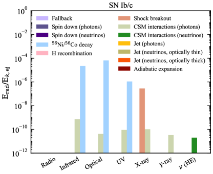
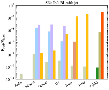
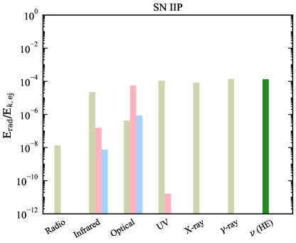
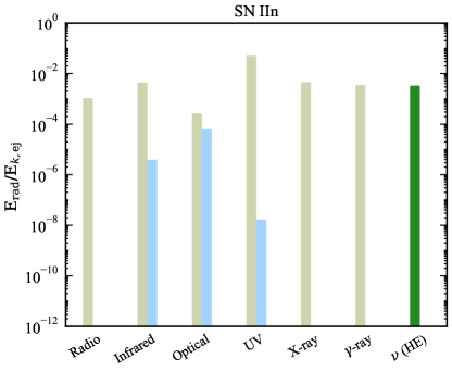
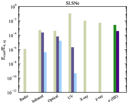
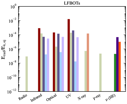
Figure 4: Ratio of the energy radiated across electromagnetic wavebands and in neutrinos (Eq. 4) and the kinetic energy of the ejecta (or energy of the jet) for SNe Ib/c, SNe Ib/c BL with jet, SNe II-P, SNe IIn, SLSNe and LFBOTs (from top left to bottom right, respectively). The color code for each process is the same as in Fig. 2. For each transient, we assume the fiducial parameters in Table 2. If the transient is engine driven, then the bulk of radiation is emitted in the UVOIR band through either fallback of matter onto the BH or the magnetar spin down. In the case of successful jet (GRB), most of the energy is emitted in the X-ray/gamma-ray bands, whereas a dimmer flash of light in the same bands resulting from shock breakout is expected for unsuccessful jets. If a dense CSM surrounds the collapsing star, then a significant fraction of energy is radiated in the UVOIR, radio and X-ray bands. In this case, also bright gamma-ray and neutrino signals are expected. Finally, when the heating source is either radioactive ⁵⁶Ni decay or H recombination, the outflow radiates energy in the UVOIR band.

V.2 Supernovae of Type IIP

Type IIP SNe originate from red supergiants, massive stars which retain the extended hydrogen envelope. The abundance of hydrogen in their progenitor may cause the plateau of variable duration observed in the light curve of these SNe due to hydrogen recombination (Hamuy, 2003; Smartt et al., 2009; Sanders et al., 2015; Rubin et al., 2016).

Typical values for the mass-loss rates of red supergiant stars are $\dot{M}_{w}\simeq 10^{-6}$–$10^{-5}\;M_{\odot}$ yr^-1, with wind velocity $v_{w}\simeq 10$ km s^-1 Margutti et al. (2017). Nevertheless, larger CSM densities are inferred from the observation of SNe IIP, with $\dot{M}_{w}\simeq\mathcal{O}(10^{-3})\;M_{\odot}$ yr^-1 (Nakaoka et al., 2018; Yaron et al., 2017; Bullivant et al., 2018). Such large densities can be explained invoking eruptive mass loss of the progenitor star $\simeq\mathcal{O}(1)$ year before the SN explosion (Morozova et al., 2017; Wagle and Ray, 2020; Nakaoka et al., 2018). Besides hydrogen recombination, ⁵⁶Ni decay can heat the SN outflow, together with CSM interactions. Recent work shows that $f_{\rm{Ni}}\equiv M_{\rm{Ni}}/M_{\rm{ej}}\lesssim 0.05$ Müller et al. (2017), thus the contribution from the radioactive decay of ⁵⁶Ni is expected to be subleading.

The total energy radiated across all electromagnetic wavebands and the neutrino energy budget are shown in Fig. 4 (middle left panel) for the parameters in Table 2. The bulk of energy radiated in the UVOIR band is produced through CSM interactions ($E^{\rm{UVOIR}}/E_{k,\rm{ej}}\simeq 10^{-4}$) and hydrogen recombination ($E^{\rm{UVOIR}}/E_{k,\rm{ej}}\simeq 6\times 10^{-5}$). Significant X-ray emission is also expected due to bremmsthralung as the ejecta propagate in the optically thin CSM ($E^{\rm{X-ray}}/E_{k,\rm{ej}}\simeq 7\times 10^{-5}$). These results depend on the assumption of eruptive mass-loss episodes prior to the stellar collapse. If typical mass-loss rates of red supergiants were adopted, the energy in the UVOIR band would be radiated through hydrogen recombination and the X-ray energy would be a negligible fraction of the explosion energy. This may be the case for most of the SNe IIP, as suggested by the lack of X-ray bright SNe IIP (Dwarkadas, 2014). Due to the large CSM density, neutrinos are produced with $E^{\nu}/E_{k,\rm{ej}}\simeq 10^{-4}$.

V.3 Supernovae of Type IIn

Type IIn SNe show clear signs of strong CSM interactions and some of them may linked to luminous blue variable, red supergiants or yellow hypergiant stars Smith (2017); Taddia et al. (2013). The mass-loss rate of the surrounding CSM ranges between $\dot{M}=10^{-4}$–$10\;M_{\odot}$ yr¹ (Smith, 2014; Moriya et al., 2014), with wind velocity $v_{w}\simeq 30$–$600$ km s^-1. As a result of the dense CSM, this class of SNe exhibits signs of strong CSM interactions.

We consider CSM interactions and ⁵⁶ Ni decay as the main processes contributing to the heating of the outflow. The results are shown in Fig. 4 (middle left panel) for the parameters in Table 2. The bulk of energy is emitted in the UVOIR band and it is produced by CSM interactions, with $E^{\rm{UVOIR}}/{E_{k,\rm{ej}}}\simeq 4\times 10^{-2}$. A significant amount of energy is also emitted through non-thermal processes in the radio ${E}^{\rm{Radio}}/{E_{k,\rm{ej}}}\simeq 10^{-3}$ and X-ray bands ${E}^{\rm{X-ray}}/{E_{k,\rm{ej}}}\simeq 5\times 10^{-3}$. Due to the large CSM density, $E^{\nu}/E_{k,\rm{ej}}\simeq 3.3\times 10^{-3}$.

V.4 Superluminous supernovae

SLSNe are an emerging class of SN explosions whose optical luminosity is ten or more times larger than standard core-collapse SNe Gal-Yam (2019). They can be broadly classified as H-poor (Type I) and H-rich (Type II) SLSNe; the lightcurve of many H-rich SLSNe is consistent with the interaction of the SN outflow with a dense CSM (Moriya et al., 2018), similarly to the case of SNe IIn. The mechanism powering Type I SLSNe is not clear, even though observations suggest that these transients may be powered by a magnetar (Kasen and Bildsten, 2010; Dexter and Kasen, 2013), which would explain the observed large kinetic energy of the outflow and radiation output (Quimby et al., 2011; Gal-Yam, 2012). On the contrary, Type II SLSNe exhibit signs of strong CSM interactions, like SNe IIn, and they are thought to be powered by CSM interactions (Smith et al., 2010). Since hybrid mechanisms invoking magnetar spin down, CSM interactions and ⁵⁶Ni decay can also be considered for this class of transients, we include all these heating sources Chen et al. (2017); Inserra et al. (2017).

The energy radiated across the electromagnetic wavebands and neutrinos is displayed in Fig. 4 (bottom left panel) for the parameters in Table 2. Most of the energy is radiated in the UVOIR band, thanks to interactions with the CSM (${E}^{\rm{UVOIR}}/{E}_{k,\rm{ej}}\simeq 10^{-1}$) and spin down of the magnetar (${E}^{\rm{UVOIR}}/{E}_{k,\rm{ej}}\simeq 2.4\times 10^{-4}$). A significant amount of energy is also emitted in X-rays through bremmstrahlung (${E}^{\rm{X-ray}}/{E}_{k,\rm{ej}}\simeq 10^{-2}$). Due to the large CSM density, a bright neutrino counterpart is expected. Furthermore, neutrinos can be produced in the magnetar wind. The fraction of energy radiated in neutrinos is $E^{\nu}/E_{k,\rm{ej}}\simeq 2\times 10^{-3}$ ($E^{\nu}/E_{k,\rm{ej}}\simeq 4\times 10^{-4}$) for CSM interactions (for the magnetar wind).

V.5 Luminous fast blue optical transients

Luminous FBOTs (LFBOTs, namely FBOTs with optical luminosity $L_{\rm{opt}}\gtrsim 10^{44}$ erg s^-1) are an emerging SN-like class reaching peak luminosity in less than $10$ days (Drout et al., 2014; Arcavi et al., 2016; Tanaka et al., 2016; Pursiainen et al., 2018), whose observed outflow asymmetry and variability of the X-ray light curve hint towards the presence of a compact object (Ho et al., 2019; Margutti et al., 2019; Gottlieb et al., 2022b). The latter should be responsible for the ejection of the observed asymmetric and fast outflow (Margutti et al., 2019; Maund et al., 2023).

One of the scenarios proposed to explain LFBOT observations invokes the collapse of a massive star, followed by the launch of a jet which inflates the cocoon (Gottlieb et al., 2022b). The star may not be completely depleted of hydrogen, thus the jet may fail in breaking out and be choked in the stellar mantle. This scenario would explain the lack of direct association between gamma-rays and LFBOTs (Bietenholz et al., 2020), as well as the asymmetric outflow and the hydrogen lines observed in the spectra of some LFBOTs (Perley et al., 2019; Margutti et al., 2019; Coppejans et al., 2020).

Radio observations suggest that a fast blastwave drives the shock moving with $v_{\rm{sh}}\gtrsim 0.1c$ in the dense CSM, extended up to $R_{\rm{CSM}}\gtrsim 10^{16}$ cm. Even though observations reveal an asymmetric CSM, using the normalization in Eq. 18, $M_{w}\simeq 10^{-4}$–$10^{-3}$ M_⊙ yr^-1 is inferred, for a wind velocity $v_{w}\simeq 1000$ km s^-1 (Ho et al., 2019; Margutti et al., 2019; Coppejans et al., 2020).

The energy radiated across the electromagnetic wavebands and in neutrinos is shown in Fig. 4 (bottom right panel). We rely on the benchmark parameters in Table 2 and consider CSM interactions, ⁵⁶Ni decay, magnetar spin down, matter fallback, and shock breakout from a massive star that is not completely hydrogen stripped star. Additionally, we consider the possibility that radiation is emitted through the adiabatic expansion of the ejecta (Gottlieb et al., 2022b), whose output luminosity is described by the homogeneous solution in Eq. 3. However, we warn the reader that the mechanism powering LFBOTs is still uncertain and that they may not be linked to collapsing massive stars, see e.g. Ref. (Metzger, 2022).

Following Ref. (Guarini et al., 2022a), we consider CSM interactions and a jet choked in an extended envelope surrounding the progenitor core as sites of neutrino production. We show the most optimistic scenario considered in Ref. (Guarini et al., 2022a) as a representative case, however the results are model dependent. The assumed total energy of the explosion only holds if LFBOTs originate from the core collapse of a massive star, whereas different origin (e.g. cf. Ref. (Metzger, 2022)) may affect the energy budget considered in this work.

From Fig. 4, we deduce that most of the energy is emitted in the UVOIR band, with ${E}^{\rm{UVOIR}}/{E}_{k,\rm{ej}}\simeq 1.6\times 10^{-2}$ (${E}^{\rm{UVOIR}}/{E}_{k,\rm{ej}}\simeq 5\times 10^{-4}$), through adiabatic expansion of the outflow (magnetar spin down). Radioactive decay of ⁵⁶Ni does not contribute significantly to the emitted radiation in the UVOIR band (Perley et al., 2019). This is consistent with the model outlined in Ref. (Gottlieb and Globus, 2021), where most of the energy is radiated through the cooling of the cocoon inflated as the jet propagates in the stellar envelope. Consistently with observations, synchrotron radiation from accelerated electrons is responsible for the observed radio emission (Margutti et al., 2019; Coppejans et al., 2020; Ho et al., 2019), with ${E}^{\rm{Radio}}/E_{k,\rm{ej}}\simeq 10^{-7}$. Neutrinos can be produced through CSM interactions and in the magnetar wind, with $E^{\nu}/E_{k,\rm{ej}}\simeq 2\times 10^{-7}$ and $E^{\nu}/E_{k,\rm{ej}}\simeq 5\times 10^{-5}$, respectively. For the assumed choked jet scenario, neutrinos are produced with $E^{\nu}/E_{k,\rm{ej}}\simeq 10^{-5}$.

VI Connection between electromagnetic emission and neutrinos

In this section, we investigate the correlation between electromagnetic radiation and neutrinos from transient sources resulting from massive stars. Since neutrino emission is expected for sources powered by the magnetar spin down, CSM interactions or sources harboring a jet, we focus on these scenarios. The magnetar spin down could be applied to the case of SLSNe and LFBOTs. On the other hand, SNe IIn, IIp, SLSNe as well as LFBOTs may have efficient CSM interactions. Efficient neutrino production is also expected in GRB jets and in jets smothered in an extended envelope, which may be the case for LFBOTs.

If the CSM is not very dense, a small fraction of the ejecta kinetic energy is radiated in neutrinos and the neutrino counterpart is not bright enough to be detected. This may be the case for non-jetted SNe Ib/c or SNe IIP which do not show signs of strong CSM interactions. Therefore, if the observed transient is only powered by ⁵⁶Ni decay or hydrogen recombination and does not show any signs of engine or CSM interactions, we expect the corresponding neutrino signal to be negligible and do not discuss this case further.

VI.1 Magnetar spin down: Superluminous supernovae and fast blue optical transients

A magnetar could power the emission of SLSNe and LFBOTs (see Fig. 4). As the spin down of the magnetar powers bright UVOIR radiation, we can correlate the neutrino signal with the electromagnetic signal.

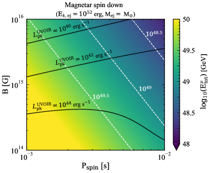
Figure 5: Isocontours of the total energy radiated in neutrinos ${E}_{\rm{tot}}^{\nu}$ (Eq. IV.3) for transients whose UVOIR lightcurve is powered by the magnetar spin down, in the plane spanned by the magnetar spin $P_{\rm{spin}}$ and magnetic field $B$. The brown dashed isocontours are displayed to guide the eye. The solid black isocontours mark benchmark values for the peak of the UVOIR luminosity, which is degenerate with respect to ($P_{\rm{spin}},B$). For a transient whose UVOIR lightcurve is powered by the magnetar spin down, the expected energy radiated in neutrinos can be inferred by localizing the transient in this plane.

Figure 5 shows contours for the total energy radiated in neutrinos from the magnetar wind (Eq. IV.3), in the plane spanned by the magnetar spin $P_{\rm{spin}}$ and the magnetic field $B$. The black solid lines mark the values of the peak bolometric luminosity in the UVOIR band for each ($P_{\rm{spin}},B$) pair. The results are shown for ${E}_{k,\rm{ej}}=10^{52}$ erg and $M_{\rm{ej}}=M_{\odot}$, however Eq. IV.3 should be used for a given kinetic energy and mass of the ejecta. These parameters can be inferred from the bolometric lightcurve, which gives information on the photospheric velocity and the rise time; the former scales as $v_{\rm{ph}}\propto\sqrt{E_{k,\rm{ej}}/v_{\rm{ej}}}$, while the latter goes like $t_{\rm{rise}}\simeq t_{\rm{d}}\propto\sqrt{M_{\rm{ej}}}$.

The peak luminosity ($L_{\rm{pk}}^{\rm{UVOIR}}$) is degenerate with respect to the ($P_{\rm{spin}},B$) pairs. The only way to break this degeneracy is to complement the information from the UVOIR band with the non-thermal signal produced by the compact object observable in the X-ray band. To a first approximation, the total energy of non-thermal photons is proportional to the magnetic field $E_{\rm{n-th}}\propto B^{-2}$, whereas it is independent on the spin $P_{\rm{spin}}$ (Fang and Metzger, 2017). Note that we have not considered the non-thermal signal in Sec. II, as its modeling is affected by large theoretical uncertainties (see Ref. (Fang and Metzger, 2017) for details).

The total energy radiated in neutrinos ($E^{\nu}_{\rm{tot}}$) from a transient powered by the magnetar spin down can be obtained from Eq. IV.3, with the characteristic parameters inferred combining observations in the UVOIR and X-ray bands. From Fig. 5 we conclude that sources with a bright UVOIR signal consistent with the spin down of a magnetar are expected to produce a very bright neutrino counterpart. Intriguingly, if neutrinos should be detected in coincidence with the UVOIR signal, the total energy emitted in neutrinos can be combined with the peak of the bolometric UVOIR lightcurve to break the degeneracy between $P_{\rm{spin}}$ and $B$, as shown in Fig. 5.

Note that we consider time-integrated quantities, yet neutrino production in the magnetar wind starts later than the UVOIR radiation, at $t_{\nu,\rm{in}}\simeq 1.4\times 10^{5}\eta_{-1}^{8/25}B_{14}^{-18/25}M_{\rm{ej},-2}^{9/50}P_{\rm{spin},-3}^{9/25}\epsilon_{B,-2}^{8/25}$ s. The neutrino flux is expected to be maximum at $t_{\nu,\rm{max}}\simeq 9.3\times 10^{5}\eta^{1/3}_{-1}B^{-2/3}_{14}M_{\rm{ej},-2}^{1/4}P_{\rm{spin},-3}^{1/2}\epsilon_{B,-2}^{1/6}$ s. This time does not correspond to the peak of the UVOIR light curve, which is expected around $10$–$100$ days (Villar et al., 2017). For example, for the benchmark transient in Fig. 2, the neutrino signal peaks at $t\simeq 34$ days when the production of thermal UVOIR radiation already stopped. Therefore, the search for neutrinos from a magnetar-powered transient should be performed for $t_{\nu,\rm{in}}\lesssim t\lesssim t_{{\nu},\rm{max}}$.

VI.2 Circumstellar interactions: Supernovae IIP, IIn, superluminous supernovae, and luminous fast blue optical transients

When the observed transient exhibits strong signs of CSM interactions in the UVOIR light curve, bright radio and X-ray counterparts are expected— modulo absorption processes taking place in the CSM—together with high-energy neutrinos; see also Refs. Katz et al. (2011); Murase et al. (2011). Here, we focus on the relation existing between the synchrotron radio and neutrino signals produced by the decelerating blastwave. This case is of relevance for SNe IIP and IIn, SLSNe, and LFBOTs (see Fig. 4).

For these transients a direct temporal correlation between the synchrotron radio and neutrino signals can be established, since both signals are produced through non-thermal processes in the proximity of the same blastwave. As the outflow propagates in the dense CSM, the forward shock converts its kinetic energy into internal energy, whose density at each time $t$ is given by Eq. 24. The energy density stored in protons is

$$u_{p}(t)\simeq E_{p}^{2}\frac{{\rm{d}}N_{p}}{{\rm{d}}E_{p}{\rm{d}}V}\simeq\epsilon_{p}\frac{u_{\rm{int}}}{\ln({E_{p,\max}/E_{p,\min}})}\;,$$ (30)

where we assume the injection spectrum given by Eq. 26.

Neutrinos are produced at the forward shock trough $pp$ interactions (Sec. IV). The neutrino energy density in the blastwave at each radius $R$ can be approximated as (Fang et al., 2020)

$${u}_{\nu}(R)\approx\frac{1}{2}{u}_{p}\left(1-e^{-\tau_{pp}}\right)\;,$$ (31)

where $u_{p}$ is given in Eq. 30 and ${\tau}_{pp}$ is the optical depth of relativistic protons. The latter is given by $\tau_{\rm{pp}}\approx\sigma_{\rm{pp}}n_{p,\rm{CSM}}R_{\rm{sh}}$ for $E_{p}=E_{p,\max}$, while $\tau_{pp}=t_{\rm{dyn}}/t_{pp}$ for $E_{p}\ll E_{p,\max}$. Here, $E_{p,\max}$, $t_{\rm{dyn}}$ and $t_{pp}$ are the maximum energy, the dynamical and $pp$ interaction timescales of protons accelerated at the external shock, respectively; see Appendix A. Finally, the cross section for $pp$ interactions is assumed to be independent of energy ($\sigma_{pp}\simeq 5\times 10^{-26}$ cm²).

The total energy emitted in neutrinos from the transient during its interaction with the CSM is

$$E_{\rm{tot}}^{\nu}=\int_{R_{\rm{bo}}}^{R_{\max}}dR4\pi R^{2}u_{\nu}(R)\;,$$ (32)

where $R_{\rm{bo}}$ is the breakout radius (Eq. 19) and $R_{\max}$ is the outer edge of neutrino production region defined as indicated in Sec. IV. From Eq. 32, we deduce that the total energy emitted by the blastwave in neutrinos is related to the upstream CSM density and the blastwave velocity at the considered time. The same dependence holds for the flux radiated in the radio band, which is produced through synchrotron losses (Margalit et al., 2022).

While the total energy radiated in neutrinos scales with $\epsilon_{p}$, the radio signal strongly depends on $\epsilon_{B}$. Thus, the ratio $E_{\rm{tot}}^{\nu}/E^{\rm{Radio}}\propto\epsilon_{p}/\epsilon_{B}$. Typical values inferred from observations are $\epsilon_{B}\simeq 10^{-3}$– $10^{-2}$ Bell and Lucek (2001), while the fraction of energy stored in protons accelerated at the forward shock is expected to be $\epsilon_{p}\lesssim 0.1$ Aharonian (2009); Helder et al. (2009). Therefore, when a bright radio source whose signal is consistent with synchrotron radiation is detected, its radio flux sets a lower limit on the total energy emitted in neutrinos by the expanding blastwave.

Figure 6 shows the contour plot of the total energy radiated in neutrinos, in the plane spanned by the upstream CSM density $n_{\rm{CSM}}$ and the blastwave dimensionless velocity $\beta_{\rm{sh}}=v_{\rm{sh}}/c$, both measured at $t=100$ days. We use $\epsilon_{p}=\epsilon_{e}=10^{-1}$ and $\epsilon_{B}=10^{-2}$ in our calculations. Radio data allow to measure the CSM density at the time $t$, while the velocity of the fastest component of the ejecta $\beta_{\rm{sh}}$ can be inferred from radio data of the transient (Chevalier and Fransson, 1994; Chevalier, 1998). A transient whose radio signal is produced through interactions of the outflow with the CSM can be located in the ($n_{\rm{CSM}},\beta_{\rm{sh}}$) plane. Once the ($n_{\rm{CSM}},\beta_{\rm{sh}}$) pair is fixed, the observed peak radio luminosity $L_{\rm{pk}}^{\rm{Radio}}$ and peak frequency $\nu_{\rm{pk}}$ can be obtained simultaneously only for a specific ($\epsilon_{B},\epsilon_{e}$) pair and vice-versa (Granot and Ramirez-Ruiz, 2004).

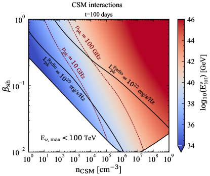
Figure 6: Isocontours of the total energy radiated in neutrinos (Eq. 32) through CSM interactions, in the plane spanned by the upstream density $n_{\rm{CSM}}$ and the shock adimensional velocity $\beta_{\rm{sh}}=v_{\rm{sh}}/c$, both measured at $t=100$ days after the explosion. The solid black (dashed purple) lines mark the peak of the radio flux $L_{\rm{pk}}^{\rm{Radio}}$ (peak frequency $\nu_{\rm{pk}}$) for $\epsilon_{B}=0.01$ and $\epsilon_{e}=0.1$. We exclude the region of the parameter space producing neutrinos with energy $E_{\nu,\max}\lesssim 100$ TeV throughout the duration of CSM interactions; see main text for details. When a transient bright in radio is detected and its light curve is consistent with synchrotron radiation, the ($n_{\rm{CSM}},\beta_{\rm{sh}}$) pair can be inferred and the expected energy radiated in neutrinos at a fixed time can be estimated from Eq. 32.

The minimum luminosity radiated in neutrinos can be inferred from radio observation as $L_{\rm{min}}^{\nu}\simeq L_{\rm{pk}}^{\rm{Radio}}\nu_{\rm{pk}}$. The total energy in neutrinos $E_{\rm{tot}}^{\nu}$ can be estimated locating the transient in the plane in Fig. 6. Otherwise, once the ($n_{\rm{CSM}},\beta_{\rm{sh}}$) pair is inferred from radio observations, the corresponding $E_{\rm{tot}}^{\nu}$ can be estimated from Eq. 32.

In summary, transients detected with a bright radio counterpart are expected to produce a bright neutrino signal. As neutrinos and radio photons are produced over the same time interval during CSM interactions (see Fig. 2), it is fundamental to identify radio sources at early times, in order to quickly initiate follow-up neutrino observations. However, we stress that the neutrino curve is expected to peak at a time likely shifted with respect to the one when the radio and optical light curves peak (Pitik et al., 2021, 2023). The procedure outlined here can be performed at different times of radio observations.

We exclude in Fig. 6 the region of the parameter space leading to the production of neutrinos with maximum energy $E_{\nu,\max}\simeq 0.05E_{p,\max}\lesssim 100$ TeV throughout the duration of CSM interactions. In fact, the neutrino events detected below $100$ TeV are contaminated by the atmospheric background and astrophysical neutrino detection would be challenging (Vitagliano et al., 2020).

If neutrinos are produced as a result of CSM interactions, then a gamma-ray counterpart should be also expected Sarmah et al. (2022, 2023). However, gamma-rays undergo $\gamma$-$\gamma$ and Bethe-Heitler processes before reaching Earth, making the correlation with the corresponding neutrino signal less straightforward.

VI.3 Jetted transients

The neutrino signal produced in the optically thin part of GRBs is strictly correlated with X-ray/gamma-ray radiation and its detectability has been extensively discussed in Ref. (Pitik et al., 2022). We refer the reader to the criterion outlined in Ref. (Guépin and Kotera, 2017) for the detectability of neutrinos from GRBs whether the bolometric X-ray/gamma-ray light curve is powered by internal shocks. The criterion does not hold if energy is dissipated through magnetic reconnection along the jet, and the correlation between neutrinos and photons is no longer trivial.

When a GRB is detected electromagnetically, correlated neutrino searches should be carried out also at energies $10^{-1}\lesssim E_{\nu}\lesssim 10^{5}$ GeV, since neutrinos may be produced in this energy range in the optically thick part of the jet (Guarini et al., 2023). Subphotospheric neutrinos could be easily differentiated from the prompt signal, as the latter peaks at energies $E_{\nu}\simeq 10^{5}-10^{6}$ GeV (Pitik et al., 2021). We note that neutrinos produced in the optically thick part of the jetted outflow do not have any direct electromagnetic counterpart, yet their detection in the direction of a GRB could be the smoking gun of the jet magnetization.

The only electromagnetic counterpart of unsuccessful jets would be the flash of light in the hard X-ray/soft gamma-ray band (Nakar and Sari, 2012; Nakar, 2015) due to the shock breakout of the cocoon, as discussed in Sec. III. Neutrinos with energy $10^{-1}\lesssim E_{\nu}\lesssim 10^{5}$ GeV  (Guarini et al., 2023) can be produced below the photosphere, if the jet is magnetized, while a neutrino signal peaking at $E_{\nu}\simeq 10^{5}$ GeV may exist if the jet is smothered in an extended envelope (Guarini et al., 2022a).

VII Detection prospects

In this section, we explore the detection prospects of neutrinos emitted from the transients considered throughout this paper (all of them already observed electromagnetically). Finally, we discuss the best strategy for follow-up searches of single transient sources and stacking searches.

VII.1 Expected number of neutrino events

In order to compute the expected number of neutrino events, where suitable, we consider IceCube-Gen2 (Aartsen et al., 2021) for representative purposes because of its large expected rate. The number of muon neutrino events expected at IceCube-Gen2 (Abbasi et al., 2021b; Aartsen et al., 2021) for a source at redshift $z$ is $N_{\nu_{\mu}}(z)=\int_{E_{\nu,\rm{min}}}^{E_{\nu,\rm{max}}}dE_{\nu}\Phi_{\nu_{\mu}}^{\rm{obs}}(E_{\nu},z)\mathcal{A}_{\rm{eff}}(E_{\nu},\delta)$, where $\mathcal{A}_{\rm{eff}}(E_{\nu},\delta)$ is the detector effective area for a source at declination $\delta$ (van Santen et al., 2022), $E_{\nu,\min}$ and $E_{\nu,\max}$ are the minimum and maximum neutrino energy, respectively. We fix $E_{\nu,\min}=100$ TeV, in order to avoid the background of atmospheric neutrinos, and choose $\delta=0^{\circ}$ to maximize the effective area of the detector. The observed fluence of muon neutrinos is $\Phi_{\nu_{\mu}}^{\rm{obs}}(E_{\nu},z)$ [in units of GeV^-1 cm^-2], calculated as outlined in Sec. IV for the model parameters in Table 2 and including neutrino flavor conversion (Anchordoqui et al., 2014; Farzan and Smirnov, 2008).

Figure 7 shows the number of muon neutrino events expected at IceCube-Gen2 as a function of the luminosity distance for SNe Ib/c BL harboring a jet, SNe IIP and IIn, SLSNe, as well as LFBOTs. For all source classes, we consider neutrino production through CSM interactions. For our fiducial parameters, CSM interactions produce neutrinos with $E_{\nu,\max}\lesssim 10^{8}$ GeV, in agreement with previous work (Murase et al., 2011, 2014; Cardillo et al., 2015; Pitik et al., 2022, 2023; Petropoulou et al., 2017; Sarmah et al., 2022; Guarini et al., 2022a).

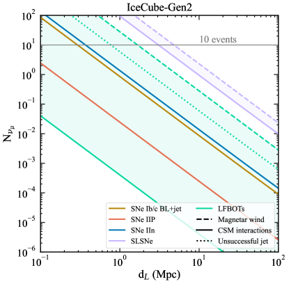
Figure 7: Expected number of muon neutrino and antineutrino events at IceCube-Gen2 as a function of the luminosity distance for SNe Ib/c BL harboring jets, SNe IIP, SNe IIn, SLSNe and LFBOTs. The gray horizontal line marks $N_{\nu_{\mu}}=10$. We consider neutrinos from CSM interactions (solid lines), from the magnetar wind (dashed lines) and from jets (dotted lines). For SNe Ib/c BL harboring a jet, we display the total number of neutrinos given by CSM interactions and the jet; CSM interactions alone produce a number of neutrinos which falls below the plotted range. CSM interactions can produce $N_{\nu_{\mu}}\simeq\mathcal{O}(10)$ at IceCube-Gen2 for SLSNe (SNe IIn) located at $d_{L}\lesssim 4$ Mpc ($d_{L}\lesssim 0.6$ Mpc). The magnetar wind can produce $N_{\nu_{\mu}}\simeq\mathcal{O}(10)$ at IceCube-Gen2 radio for SLSNe (LFBOTs) located at $d_{L}\lesssim 5$ Mpc ($d_{L}\lesssim 2$ Mpc). $N_{\nu_{\mu}}\simeq\mathcal{O}(10)$ is expected at IceCube-Gen2 from LFBOTs harboring unsuccessful jets and placed at $d_{L}\lesssim 1$ Mpc. Note that the number of neutrino events from jets, both successful and unsuccessful, is model dependent; see main text for details.

For SLSNe and LFBOTs, we also calculate the number of neutrino events expected from the magnetar wind. These neutrinos have energies larger than the ones produced through CSM interactions, with their signal expected to peak at $E_{\nu}\simeq 10^{8}$–$10^{9}$ GeV (Fang and Metzger, 2017). In this energy range the sensitivity of the radio extension of IceCube-Gen2 is better than its optical component (Aartsen et al., 2021), thus we estimate the detection perspectives of neutrinos from the magnetar wind at IceCube-Gen2 radio. In our simplified model, we assume that $N_{\nu_{\mu}}\simeq E_{\rm{rad}}^{\nu,\max}/10^{8.5}\;\rm{GeV}\mathcal{A}_{\rm{eff}}(10^{8.5}\;\rm{GeV})$, where $\mathcal{A}_{\rm{eff}}(10^{8.5}\;\rm{GeV})$ is the effective area of the radio extension IceCube-Gen2 at $\simeq 10^{8.5}$ GeV (van Santen et al., 2022). This is an approximation due to the fact that we do not consider the energy distribution of neutrinos from the magnetar.

As for SNe Ib/c BL harboring jets, we show the total number of events expected at IceCube-Gen2 in Fig. 7 from a successful jet, whereas the neutrino signal from CSM interactions only would be too small to be detected (see Sec. V). If the jet is smothered in the Wolf-Rayet star progenitor, neutrinos with $E_{\nu}\lesssim 10^{5}$ GeV may be produced; the related detection prospects of subphotospheric neutrinos havew been explored in Ref. (Guarini et al., 2023).

As outlined in Sec. V, LFBOTs may harbor jets which are smothered in the extended envelope surrounding the progenitor core (Gottlieb et al., 2022b). In this scenario, a signal peaking at $E_{{\nu}}\simeq 10^{5}$ GeV may be produced in the unsuccessful jet (Guarini et al., 2022a) (see also Ref. (Senno et al., 2016) for neutrino production in jets smothered in an extended envelope). In Fig. 7 we show the corresponding expected number of neutrino events, obtained by relying on the most optimistic model of Ref. (Guarini et al., 2022a).

From Fig. 7, we deduce that the expected number of neutrino events from CSM interactions is $N_{\nu_{\mu}}\simeq\mathcal{O}(10)$ for SLSNe (SNe IIn) located at $d_{L}\lesssim 4$ Mpc ($d_{L}\lesssim 0.6$ Mpc). Large CSM densities may be possible around SLSNe and SNe IIn, with $M_{w}\lesssim 10M_{\odot}$ yr^-1 (Smith, 2014; Moriya et al., 2014); in this case, the expected number of neutrino events from SLSNe and SNe IIn could be larger than considered here (Pitik et al., 2023). Neutrinos from magnetar winds show promising detection perspectives at IceCube-Gen2 radio, with $N_{\nu_{\mu}}\simeq\mathcal{O}(10)$ for SLSNe and LFBOTs located at $d_{L}\lesssim 5$ Mpc and $d_{L}\lesssim 2$ Mpc, respectively. Unsuccessful jets in LFBOTs may produce $N_{\nu_{\mu}}\gtrsim\mathcal{O}(10)$, if the source is at $d_{L}\lesssim 1$ Mpc. However, we note that the neutrino signal from the choked jet peaks at energies $E_{\nu}\simeq 10^{5}$ GeV and it quickly drops at larger energies (Guarini et al., 2022a), where the sensitivity of IceCube-Gen2 increases (Aartsen et al., 2021). Thus, the most promising detection prospects for LFBOT sources are obtained with IceCube, due to its sensitivity range (Abbasi et al., 2021b) (see Fig. 6 in Ref. (Guarini et al., 2022a) for the expected number of neutrinos in this case). We stress that the results for both successful and smothered jets are model dependent and the number of events is calculated assuming that the jet is observed on-axis.

In order to assess the likelihood of finding such transients and contrast the local rate with the expected number of muon neutrino events, we assume that all these sources follow the star formation rate as a function of redshift. The local rates of the sources considered throughout this paper ($\mathcal{R}_{0}$) relative to the one of core-collapse SNe—$\mathcal{R}_{0}^{\rm{CCSN}}=(1.02\times 10^{-4})^{+70\%}_{-30\%}$ Mpc^-3 yr^-1 (Margutti et al., 2014; Vitagliano et al., 2020)—are listed in Table 3.

Table 3: Local rate ($\mathcal{R}_{0}$) of the sources considered throughout this paper including their error bands, relative to the local rate of core-collapse SNe [$\mathcal{R}_{0}^{\rm{CCSN}}=(1.25\times 10^{-4})^{+70\%}_{-30\%}$ Mpc^-3 yr^-1] (Yuksel et al., 2008; Vitagliano et al., 2020). Note that the local rate of GRBs refers to GRBs beamed towards us. For reference, we also show the rate of low-luminosity (LL) GRBs as they are more abundant and might also be related to choked jets and/or shock breakouts.

Source	$\mathcal{R}_{0}/\mathcal{R}_{0}^{\rm{CCSNe}}$	Reference
SNe Ib/c	$(26\%)^{+5.1\%}_{-4.8\%}$	(Smith et al., 2011)
SNe Ib/c BL	$\lesssim 13\%$	(Corsi and Lazzati, 2021)
SNe Ib/c BL with choked jet	Unknown	(Corsi and Lazzati, 2021)
GRBs	$\lesssim 10^{-5}$	(Lien et al., 2014)
LL GRBs	$\lesssim 10^{-3}$	(Virgili et al., 2009)
SNe IIP	$(48.2\%)^{+5.7\%}_{-5.6}$	(Smith et al., 2011)
SNe IIn	$(8.8\%)^{+3.3\%}_{-2.9\%}$	(Smith et al., 2011)
SLSNe	$\lesssim 2.8\times 10^{-3}$	(Quimby et al., 2013)
LFBOTs	$\lesssim 10^{-3}$	(Coppejans et al., 2020)

SLSNe and LFBOTs display the most promising chances of neutrino detections if powered by a magnetar, however these sources are the least abundant in the local universe. Using Table 3, $\simeq 4\times\mathcal{O}(10^{-7})$ Mpc^-3 yr^-1 [ $\simeq 2\times\mathcal{O}(10^{-7})$ Mpc^-3 yr^-1 ] SLSNe (LFBOTs) are expected at $d_{L}=10$ Mpc (note that we consider the central values of the rates). On the contrary, SNe IIP are the most abundant sources locally, with $\mathcal{R}_{0}^{\rm{SN\;IIP}}=1.1\times 10^{-4}$ Mpc^-3 yr^-1. Nevertheless, their neutrino signal is too weak to be detected at IceCube-Gen2. Jetted outflows are also expected to produce a significant number of neutrinos. Yet the probability that the jet points towards us is $\theta_{j}^{2}/4\simeq\mathcal{O}(10^{-3})$ for typical opening angles (see Table 2). The beaming factor and the small local rate of GRBs, LFBOTs and SNe Ib/c BL which may harbor jets (Table 3) challenge the associated neutrino detection.

VII.2 Combining multi-messenger signals

On the basis of our findings, we now outline a possible strategy to carry out multi-messenger observations of transients originating from collapsing massive stars. As outlined in Sec. VI.2, radio sources whose signal is consistent with synchrotron radiation are expected to have a bright neutrino counterpart. SLSNe, SNE IIn, LFBOTs and SNe IIP with eruptive episodes fall in the category of transients with strong CSM interactions, as shown in Figs. 4 and 7. The synchrotron signal is the signature of a collisionless shock expanding in a dense CSM and it plays a crucial role for multi-messenger searches. First, as neutrinos and radio photons are produced over the same time interval from CSM interactions (Fig. 2), early detection of the radio signal will be crucial to swiftly initiate follow-up neutrino searches. The latter can be guided by the criterion outlined in Sec. VI.2. Since gamma-rays are also expected to be produced together with neutrinos (Kelner and Aharonian, 2008) (see Fig. 4), radio detection should also guide gamma-ray follow-up searches, e.g. with Fermi-LAT (Atwood et al., 2009) or the Cherenkov Telescope Array (CTA) (Mazin, 2020).

Sources emitting in X-rays due to bremsstrahlung emission are also hosted in a dense CSM, although this signal is produced through radiative shocks and may hint towards the existence of an asymmetric CSM (Brethauer et al., 2022). Neutrinos produced at the same site of bremmsthralung radiation have energies below the sensitivity range of IceCube and IceCube-Gen2 (Fang et al., 2020) and we have not considered them throughout this work. Yet, X-ray data from bremmsthralung can be combined with synchrotron radio data to infer the CSM properties, that affect the expected neutrino signal (Fang et al., 2020; Sarmah et al., 2023; Pitik et al., 2023).

If the UVOIR lightcurve shows signs of central magnetar activity, as it may be the case for SLSNe and LFBOTs, X-ray telescopes should look for a non-thermal and time variable signal. The latter may emerge at later times than the UVOIR light, due to the opacity of the outflow (Margutti et al., 2019). As detailed in Sec. VI.1, the non-thermal X-ray signal is key to disentangle the degeneracies plaguing the UVOIR lightcurve. Neutrino searches from this class of transients should start later than the UVOIR observations, and they should be carried out in the time window [$t_{\nu,\min},t_{\nu,\max}$] defined in Sec. VI.1, e.g. with IceCube-Gen2 radio.

Intriguingly, SLSNe and LFBOTs may be powered either by CSM interactions or magnetar spin down. While neutrinos from the former have energies $E_{\nu}<10^{8}$ GeV, a signal peaking at $E_{\nu}\gtrsim 10^{8}$ GeV is expected from the latter. The time window during which neutrinos are radiated is different and it depends on the mechanism responsible for their production (see Fig. 2). Thus, the energies and the detection time of neutrinos in the direction of the transient source can be combined with electromagnetic observations to disentangle the dominant mechanism powering the lightcurve.

Some sources, such as LFBOTs and SNe Ib/c BL, may harbor a choked jet pointing towards us. The resulting outflow has an asymmetry observable in the UVOIR and radio bands and it moves with middly-relativistic velocity, otherwise unreachable through symmetric explosions (Maeda et al., 2023). The electromagnetic signature of the choked jet would be a flash of light in the X-ray band (Nakar and Sari, 2012); see Fig. 4. Improving X-ray detection techniques to unambiguously detect shock breakouts will be crucial to model the associated neutrino signal.

If a mildly-relativistic outflow is inferred from radio observations, one should search for neutrinos in the direction of the transient hundred to thousand seconds before and after the first observation in the UVOIR band (see also Fig. 2). Indeed, if an unsuccessful jet is hidden in the source, neutrinos may be produced while the outflow is still optically thick and for a time $t_{\rm{dur}}^{\nu}\simeq t_{j}$. IceCube and IceCube-Gen2 could potentially detect neutrinos from a jet smothered in a red supergiant progenitor star, whereas IceCube DeepCore (Abbasi et al., 2012) is needed to observe neutrinos from a jet choked in Wolf-Rayet stars (Guarini et al., 2023, 2022a). A combined search may be promising for neutrinos from mildly-relativistic sources.

Finally, if the UVOIR lightcurve should mostly exhibit signs of ⁵⁶Ni decay or hydrogen recombination, the corresponding neutrino emission would be a negligible fraction [$\lesssim\mathcal{O}(10^{-13})$] of the ejecta kinetic energy. Searches of neutrinos in the direction of sources only powered through these processes would not be successful.

Table 4: Summary of our results. We list the luminosity distance ($d_{L}$) where $N_{\nu_{\mu}}=10$ for our benchmark transients (Fig. 7), the number of transients expected per year within $d_{L}$ [$N_{\rm{trans}}(\leq d_{L})$] and the best wavelength to correlate with neutrinos. The bands reflect the uncertainty on the local core-collapse SN rate (Mathews et al., 2014) and on the fraction of SNe belonging to each class (Smith et al., 2011). Note that for SNe Ib/c BL with a choked jet we calculate the number of neutrinos expected at IceCube DeepCore (Abbasi et al., 2012), by relying on the results in Ref. (Guarini et al., 2023).

Source	Model	$d_{L}$ [Mpc]	$N_{\rm{trans}}(\leq d_{L})$ [yr-1]	Best correlated wavelength
SLSNe	CSM interactions	4	$\lesssim 10^{-3}$	Radio
SLSNe	Magnetar wind	5	$\lesssim 2\times 10^{-3}$	UVOIR+X-ray
SNe IIn	CSM interactions	0.6	$3.5\times 10^{-3}-2\times 10^{-2}$	Radio
SNe IIP	CSM interactions	$0.05$	$6\times 10^{-4}-2\times 10^{-3}$	Radio
LFBOTs	Magnetar wind	2	$\lesssim 2\times 10^{-6}$	UVOIR+X-ray
LFBOTs with jet	Choked jet in extended envelope	1	$\lesssim 5\times 10^{-7}$	X-ray/gamma-ray
GRBs	Envelope of more models (Ref. (Pitik et al., 2022))	$0.2$	$\lesssim 2\times 10^{-8}$	X-ray/gamma-ray
SNe Ib/c with choked jet	Choked jet in Wolf-Rayet star	90	Unknown	X-ray/gamma-ray

VII.3 Follow-up searches for selected sources and stacking searches for a source class

The detection prospects for follow-up searches of a selected source together with the best wavelength to correlate with neutrinos for each transient are summarized in Table 4. We list the luminosity distance ($d_{L}$) where $N_{\nu_{\mu}}=10$ for our benchmark transients in Fig. 7, and the number of transients expected per year within $d_{L}$ [$N_{\rm{trans}}(\leq d_{L})$]. The bands reflect the uncertainty on the local core-collapse SN rate (Mathews et al., 2014) and the fraction of SNe belonging to each class (Smith et al., 2011). We do not include SNe Ib/c as the number of expected neutrinos from CSM interactions only is too low to be detected. For completeness, we also show the expected distance where $N_{\nu_{\mu}}=10$ at IceCube DeepCore (Abbasi et al., 2012) for jets choked in Wolf-Rayet star progenitors, by relying on the results of Ref. (Guarini et al., 2023).

In order to carry out stacking searches of neutrinos from radio-bright transients, one can search through archival all-sky neutrino data for clusters of a few neutrino events in the direction of identified radio transients. To this purpose, it would be useful to compile catalogues of transients detected in the radio band, e.g. relying on data from the Very Larger Array Sky Survey (VLASS) (Lacy et al., 2020). Additional radio catalogues will be available in the near future, through the Square Kilometer Array Observatory (SKA), which will cover the Southern hemisphere (Macquart et al., 2015). Note, however, that an appropriate weighting of the sources relative to each other is recommended in order to optimize neutrino searches Pitik et al. (2023).

Another important factor in the search for neutrinos from radio sources is the time window. As extensively discussed in this work and shown in Fig. 2, the neutrino and radio signals are produced over the same window. The peak of the neutrino signal is expected to occur not too far from the breakout time of the forward shock from the CSM, or anyway around the peak of the optical lightcurve (Pitik et al., 2023). The same results do not hold for the radio signal, whose peak can occur much later than the optical one, depending on the properties of the CSM and the forward shock. Thus, it is crucial to combine UVOIR and radio data to optimize the time window for neutrino searches.

The atmospheric neutrino background increases when a long time window is chosen. Yet the criterion presented in Fig. 6 excludes the parameter space contaminated by atmospheric neutrinos, considering only the $(n_{\rm{CSM}},\beta_{\rm{sh}})$ pairs which allow for the production of neutrinos with $E_{\nu}\gtrsim 10^{5}$ GeV. Our findings provide guidance to identify the ideal time window to carry out radio and neutrino stacking searches. We also encourage to initiate radio follow-up observations of neutrino alerts (Aartsen et al., 2017b). In order to better assess the CSM properties, follow-up observations in the X-ray bands are needed to break the degeneracies in the $(n_{\rm{CSM}},\beta_{\rm{sh}})$ space (Margalit et al., 2022).

VIII Discussion and conclusions

In this work, we consider SNe Ib/c, SNe Ib/c BL harboring jets, SNe II-P, SNe IIn, SLSNe, as well as LFBOTs and compute the energy radiated across the observable electromagnetic wavebands and neutrinos. Our findings reveal that most of the energy is radiated in the UVOIR band. However, a significant fraction of the outflow kinetic energy can be emitted either in the radio or the X-ray bands through synchrotron or bremsstrahlung processes, when a dense CSM engulfs the collpasing star. Since the UVOIR light curve is degenerate with respect to the transient model parameters, a correlation of neutrino observations with this band alone is not sufficient, in agreement with the findings of Ref. Pitik et al. (2023). However, one could combine UVOIR observations with radio data to infer upper and lower limits, respectively, on the ejecta energy $E_{\rm{ej}}$ and mass $M_{\rm{ej}}$ (Coppejans et al., 2020; Ho et al., 2019; Chevalier, 1998).

While the peak of the UVOIR luminosity of transients powered by the spin down of a magnetar is degenerate with respect to the spin period and magnetic field of the pulsar, multi-wavelength observations are fundamental to break these degeneracies. In particular, X-ray/non-thermal data can be combined with the thermal UVOIR ones to infer the spin and magnetic field (Fang and Metzger, 2017) and allow to forecast the neutrino number of events. Neutrino observations could be instrumental to break the degeneracy between the spin period and the magnetic field. As the neutrino production starts (ends) when photopion processes become efficient (inefficient), neutrino searches should be carried out in a time window uncorrelated with the UVOIR lightcurve.

Our findings reveal that bright radio sources are promising high-energy neutrino factories. Opposite to the UVOIR signal, a correlation between the radio and optical signals exist. Radio photons and neutrinos are produced over the same time interval and therefore neutrino searches should be performed over the duration of the radio emission. The radio counterpart allows to infer the CSM density $n_{\rm{CSM}}$ and the shock velocity $\beta_{\rm{sh}}=v_{\rm{sh}}/c$ at the observed time (Chevalier, 1998). The minimum neutrino luminosity expected at each emission time from the transient can be computed considering the product of the radio peak luminosity and peak frequency $E_{\rm{rad},\min}^{\nu}\simeq L_{\rm{pk}}^{\rm{Radio}}\nu_{\rm{pk}}$, and the total energy radiated in neutrinos can be localized in the plane spanned by $n_{\rm{CSM}}$ and $\beta_{\rm{sh}}$.

For our fiducial parameters, IceCube-Gen2 will be able to detect neutrinos from SLSNe at $d_{L}\lesssim 4$ Mpc, when neutrinos are produced from CSM interactions. If SLSNe (LFBOTs) harbor a central magnetar, $10$ neutrino events produced in the magnetar wind are expected in IceCube-Gen2 radio for sources at $d_{L}\lesssim 5(2)$ Mpc.

While transients linked to massive stars are routinely detected in the UVOIR band, our findings urge to optimize the detection opportunities in the radio and X-ray bands to swiftly identify CSM and magnetar powered transients. Furthermore, neutrino searches would be useful for mildly-relativistic transients, as neutrinos may signal the presence of a choked jet. Improving observational techniques in the UV/X-ray will be fundamental to detect the shock breakout light and model the corresponding neutrino signal. Neutrino searches from mildly-relativistic sources should be performed $\mathcal{(}10$–$1000)$ s before and after the first UVOIR signal.

In summary, in order to optimize the chances of joint detection of electromagnetic radiation and neutrinos from transients stemming from collapsing massive stars, follow-up programs solely based on UVOIR observations are not optimal. UVOIR data should be complemented by radio data tracing CSM interactions or X-ray data carrying imprints of the activity of the central engine, if any. Only exploiting multi-wavelength and neutrino data can we explore the physics powering these fascinating sources and properly guide multi-messenger follow-up programs.

Appendix A Interaction rates of accelerated protons

In this appendix we summarize the interaction rates of protons accelerated in the magnetar wind as well as at CSM interactions or in a jetted outflow.

A.1 Magnetar wind

The energy deposited by the spin down is partially deposited into kinetic energy of the outflow, with the remaining energy being used to produce thermal and non-thermal radiation. Therefore, protons accelerated in the magnetar wind interact through $p\gamma$ interactions both with thermal and non-thermal photons in the wind nebula. The corresponding interaction rates are (Fang and Metzger, 2017):

$$t^{-1}_{p\gamma,\rm{th}} = 7.7\times 10^{-5}t_{5.5}^{-15/8}B_{14}^{-3/4}\beta_{w}^{-15/8}\;\rm{s}\;,$$ (33)

$$t^{-1}_{p\gamma,\rm{nth}} = 2.4\times 10^{-5}t_{5.5}^{-27/8}B_{14}^{-7/4}\beta_{w}^{-19/8}\;\rm{s}\;,$$ (34)

where $\beta_{w}\simeq 1M_{\rm{ej},-2}^{-1/2}P_{\rm{spin},-3}^{-1}$ is the wind velocity after its acceleration, at times $t\gg t_{\rm{sd}}$, where $t_{\rm{sd}}$ is the spin-down time defined as in Eq. 10.

The interaction rate for $pp$ interactions is

$$t_{pp}^{-1}=6.25\times 10^{-9}M_{\rm{ej},-2}^{-1}t_{5.5}^{3}\beta_{w}^{3}\;\rm{s}\;.$$ (35)

Pions are created in the wind nebula at a rate

$$t^{-1}_{\pi,\rm{cre}}=t^{-1}_{p\gamma,\rm{th}}+t^{-1}_{p\gamma,\rm{nth}}+t^{-1}_{pp}\;.$$ (36)

The only proton cooling process competing with pion production is the synchrotron cooling, whose characteristic time is

$$t_{p,\rm{rad}}=5.6\times 10^{-6}\eta^{-1}_{-1}t_{5.5}^{5}B^{3}_{14}\beta_{w}^{3}\epsilon_{B,-2}^{-1}\;\rm{s}.$$ (37)

Thus, pion creation in the wind nebula is suppressed by a factor

$$f^{p}_{\rm{sup}}=\min\left(1,\frac{t_{\rm{ad}}}{t_{\pi,\rm{cre}}},\frac{t_{p,\rm{rad}}}{t_{\pi,\rm{cre}}}\right)\,$$ (38)

where $t_{\rm{ad}}\simeq R/\beta_{w}c$ is the adiabatic expansion time scale of the wind nebula.

The onset of neutrino production corresponds to the time when efficient photopion production starts, namely when $t_{p,\rm{rad}}^{-1}\equiv t_{\pi,\rm{cre}}^{-1}$. Similarly, neutrino production ends at the time when photopion processes are no longer efficient, i.e. $t_{\pi,\rm{cre}}^{-1}\equiv t_{\rm{cross}}^{-1}$.

Before decaying, secondary pions and muons also cool. Their cooling affects the neutrino signal through the following suppression factors:

$$f^{\pi}_{\rm{sup}} = 0.3\eta_{-1}^{-2}B_{14}^{4}\epsilon_{B,-2}^{-1}t_{5.5}^{6}\;,$$ (39)

$$f^{\mu}_{\rm{sup}} = 1.5\times 10^{-3}\eta_{-1}^{-2}B_{14}^{4}\beta_{w}^{3}\epsilon_{B,-2}^{-1}t_{5.5}^{6}\;.$$ (40)

A.2 CSM interactions and jets

In the case of non-relativistic and mildly relativistic shocks—such as the external shock driven by the outflow as it expands in the CSM—the proton acceleration rate is obtained from the Bohm limit (Protheroe and Clay, 2004)

$$t^{\prime-1}_{\rm{acc}}\simeq\frac{3eBv_{\rm{sh}}^{2}}{20\gamma_{p}m_{p}c^{3}}\;,$$ (41)

where $e=\sqrt{\hbar\alpha c}$ is the elementary electric charge, $\alpha=1/137$ is the fine structure constant and $\hbar$ is the reduced Planck constant; for non-relativistic shocks, the comoving frame of the outflow and the center of explosion frame coincide—we carry out the calculations in the comoving frame of the outflow and we denote quantities with $X^{\prime}$. The magnetic field $B$ is defined as in Sec. II and $\gamma_{p}$ is the proton Lorentz factor.

In the case of relativistic and mildly relativistic outflows, the proton acceleration rate is

$$t^{\prime-1}_{\rm{acc}}=\frac{ceB^{\prime}}{\xi E^{\prime}_{p}}\;,$$ (42)

where $\xi$ represents the number of gyroradii needed for accelerating protons. We assume $\xi=10$ (Gao et al., 2012). Finally, $B^{\prime}$ is the magnetic field along the jet, which depends on the energy dissipation mechanism (Pitik et al., 2021).

The total cooling rate of accelerated protons is

$$t^{{}^{\prime}-1}_{p,\rm{cool}}=t^{{}^{\prime}-1}_{\rm{ad}}+t^{{}^{\prime}-1}_{p,\rm{sync}}+t^{{}^{\prime}-1}_{p\rm{\gamma}}+t^{{}^{\prime}-1}_{pp}+t^{{}^{\prime}-1}_{p,\rm{BH}}+t^{{}^{\prime}-1}_{p,\rm{IC}}\ ,$$ (43)

where $t^{{}^{\prime}-1}_{\rm{ad}}$, $t^{{}^{\prime}-1}_{p,\rm{sync}}$, $t^{{}^{\prime}-1}_{p\gamma}$, $t^{{}^{\prime}-1}_{{pp}}$, $t^{{}^{\prime}-1}_{p,\rm{BH}}$, $t^{{}^{\prime}-1}_{p,\rm{IC}}$ are the adiabatic, synchrotron, photo-hadronic ($p\gamma$), hadronic ($pp$), Bethe-Heitler (BH, $p\gamma\rightarrow pe^{+}e^{-}$) and inverse Compton (IC) cooling rates, respectively, defined as follows (Dermer and Menon, 2009; Gao et al., 2012; Razzaque et al., 2005):

$$t^{\prime-1}_{\rm{ad}} = \frac{v}{R}\ ,$$ (44)

$$t^{\prime-1}_{p,\rm{sync}} = \frac{4\sigma_{T}m_{e}^{2}E^{\prime}_{p}B^{\prime 2}}{3m_{p}^{4}c^{3}8\pi}\ ,$$ (45)

$$t^{\prime-1}_{p\gamma} = \frac{c}{2\gamma^{\prime 2}_{p}}\int_{E_{\rm{th}}}^{\infty}dE^{\prime}_{\gamma}\frac{n^{\prime}_{\gamma}(E^{\prime}_{\gamma})}{E^{\prime 2}_{\gamma}}$$

$$\;\times\int_{E_{\rm{th}}}^{2\gamma^{\prime}_{p}E^{\prime}_{\gamma}}dE_{r}E_{r}\times\sigma_{p\gamma}(E_{r})K_{p\gamma}(E_{r})\ ,$$

$$t^{\prime-1}_{{pp}} = cn^{\prime}_{p}\sigma_{pp}K_{pp}\ ,$$ (47)

$$t^{\prime-1}_{p,\rm{BH}} = \frac{7m_{e}\alpha\sigma_{T}c}{9\sqrt{2}\pi m_{p}\gamma^{\prime 2}_{p}}\int_{\gamma_{p}^{\prime-1}}^{\frac{E^{\prime}_{\gamma,\rm{max}}}{m_{e}c^{2}}}d\epsilon^{\prime}\frac{n^{\prime}_{\gamma}(\epsilon^{\prime})}{\epsilon^{{}^{\prime}2}}$$

$$\;\times\biggl{\{}(2\gamma^{\prime}_{p}\epsilon^{\prime})^{3/2}\biggl{[}\ln(\gamma^{\prime}_{p}\epsilon^{\prime})-\frac{2}{3}\biggr{]}+\frac{2^{5/2}}{3}\biggr{\}}\ ,$$

$$t^{\prime-1}_{p,\rm{IC}} = \frac{3(m_{e}c^{2})^{2}\sigma_{T}c}{16\gamma_{p}^{\prime 2}(\gamma^{\prime}_{p}-1)\beta^{\prime}_{p}}\int_{E^{\prime}_{\gamma,\rm{min}}}^{E^{\prime}_{\gamma,\rm{max}}}\frac{dE^{\prime}_{\gamma}}{E_{\gamma}^{{}^{\prime}2}}$$

$$\;\times F(E^{\prime}_{\gamma},\gamma^{\prime}_{p})n^{\prime}_{\gamma}(E^{\prime}_{\gamma})\ ,$$

where $v=2c\Gamma$ for the jetted outflow and $v=v_{\rm{sh}}$ for CSM interactions, $\gamma_{p}=E^{\prime}_{p}/m_{p}c^{2}$ is the proton Lorentz factor, $\epsilon^{\prime}=E^{\prime}_{\gamma}/m_{e}c^{2}$, $E_{\rm{th}}=0.150$ GeV is the energy threshold for photo-pion production, and $\beta^{\prime}_{p}\approx 1$ for relativistic particles. The function $F(E^{\prime}_{\gamma},\gamma^{\prime}_{p})$ is defined in Ref. Jones (1965), with the replacement $m_{e}\rightarrow m_{p}$. The cross sections for $p\gamma$ and $pp$ interactions, $\sigma_{p\gamma}$ and $\sigma_{pp}$ are taken from Ref. Zyla et al. (2020). The function $K_{p\gamma}(E_{r})$ is the inelasticity of $p\gamma$ interactions defined in Eq. 9.9 of Dermer and Menon (2009):

$$K_{p\gamma}(E_{r})=\left\{\begin{array}[]{@{}l@{}}0.2\;\;\;\;\;\;\;\;\;E_{\rm{th}}<E_{r}<1~{}\rm{GeV}\\ 0.6\;\;\;\;\;\;\;\;\;E_{r}>1~{}\rm{GeV}\ ,\end{array}\right.\$$ (50)

with $E_{r}=\gamma^{\prime}_{p}E^{\prime}_{\gamma}(1-\beta^{\prime}_{p}\cos\theta^{\prime})$ being the relative energy between a proton with Lorentz factor $\gamma^{\prime}_{p}$ and a photon with energy $E^{\prime}_{\gamma}$, which move in the comoving frame of the interaction region along directions which form an angle $\theta^{\prime}$. The comoving proton density is $n^{\prime}_{p}={E}_{\rm{iso}}/(4\pi R_{j}^{2}c{t}_{j}\Gamma^{2})$ for the jetted outflow, and $n^{\prime}_{p}=4n_{p,\rm{CSM}}m_{p}c^{2}$ for CSM interaction. The inelasticity of $pp$ interactions is $K_{pp}=0.5$ and $n^{\prime}_{\gamma}(E^{\prime}_{\gamma})$ is the photon target for accelerated protons, defined in the main text for the jetted and spherical outflow. Before decaying, also secondary pions and muons cool through synchrotron, adiabatic and hadronic energy losses. Their cooling rates are defined as for protons, but replacing $m_{p}\rightarrow m_{x}$, with $m_{x}$ being the mass of the $x$ secondary particle.

Appendix B Radiative shocks

When the gas behind the shock immediately cools in a thin shell, the shocks are radiative. This happens when the CSM density is very large (Fang et al., 2020; Margalit et al., 2022). Also in the radiative regime the dynamical timescale for the forward shock driven by the outflow in the optically thin CSM is $t_{\rm{dyn}}=R/v_{\rm{sh}}$.

When the forward shock breaks out from the dense CSM shell, bremmstrahlung becomes the leading mechanisms for photon production and electrons mainly cool through free-free emission. The timescale for this process reads

$$t_{\rm{ff}}=\frac{3n_{e}k_{B}T_{e}}{2\Lambda_{\rm{ff}}(n_{e},T_{e})}\;,$$ (51)

where $\Lambda_{\rm{ff}}$ is the free-free cooling rate (Draine, 2011), $k_{B}T_{e}=3/16\mu_{p}m_{p}v_{\rm{sh}}^{2}$ is the post-shock temperature of the gas, with $\mu_{p}\simeq 0.62$ being the mean molecular weight for a fully-ionized gas. The post-shock electron density is $n_{e}=4\rho_{\rm{CSM}}m_{p}/\mu_{e}$ and $\mu_{e}\simeq 1.18$. Finally, $L_{\rm{sh}}=2\pi R_{\rm{CSM}}^{2}\rho_{\rm{CSM}}(R_{\rm{CSM}})v_{\rm{sh}}^{3}$ is the total kinetic shock power computed at the CSM edge.

References

- Janka (2012) H.-T. Janka, Ann. Rev. Nucl. Part. Sci. 62, 407 (2012), arXiv:1206.2503 [astro-ph.SR] .
- Woosley (1993) S. E. Woosley, Astrophys. J. 405, 273 (1993).
- MacFadyen and Woosley (1999) A. MacFadyen and S. E. Woosley, Astrophys. J. 524, 262 (1999), arXiv:astro-ph/9810274 .
- Woosley and Bloom (2006) S. E. Woosley and J. S. Bloom, Ann. Rev. Astron. Astrophys. 44, 507 (2006), arXiv:astro-ph/0609142 .
- Gehrels et al. (2009) N. Gehrels, E. Ramirez-Ruiz, and D. B. Fox, Ann. Rev. Astron. Astrophys. 47, 567 (2009), arXiv:0909.1531 [astro-ph.HE] .
- Kaneko et al. (2006) Y. Kaneko, E. Ramirez-Ruiz, J. Granot, C. Kouveliotou, S. E. Woosley, S. K. Patel, E. Rol, J. J. M. i. Zand, R. A. M. J. Wijers, and R. Strom, Astrophys. J. 654, 385 (2006), arXiv:astro-ph/0607110 .
- Drout et al. (2014) M. R. Drout et al., Astrophys. J. 794, 23 (2014), arXiv:1405.3668 [astro-ph.HE] .
- Arcavi et al. (2016) I. Arcavi et al., Astrophys. J. 819, 35 (2016), arXiv:1511.00704 [astro-ph.CO] .
- Tanaka et al. (2016) M. Tanaka et al., Astrophys. J. 819, 5 (2016), arXiv:1601.03261 [astro-ph.HE] .
- Pursiainen et al. (2018) M. Pursiainen et al. (DES), Mon. Not. Roy. Astron. Soc. 481, 894 (2018), arXiv:1803.04869 [astro-ph.HE] .
- Ho et al. (2023) A. Y. Q. Ho et al., Astrophys. J. 949, 120 (2023), arXiv:2105.08811 [astro-ph.HE] .
- Quimby et al. (2011) R. M. Quimby et al., Nature 474, 487 (2011), arXiv:0910.0059 [astro-ph.CO] .
- Gal-Yam (2019) A. Gal-Yam, Ann. Rev. Astron. Astrophys. 57, 305 (2019), arXiv:1812.01428 [astro-ph.HE] .
- Milisavljevic et al. (2015a) D. Milisavljevic et al., Astrophys. J. 815, 120 (2015a), arXiv:1511.01907 [astro-ph.HE] .
- Margutti et al. (2017) R. Margutti et al., Astrophys. J. 835, 140 (2017), arXiv:1601.06806 [astro-ph.HE] .
- Villar et al. (2017) V. A. Villar, E. Berger, B. D. Metzger, and J. Guillochon, Astrophys. J. 849, 70 (2017), arXiv:1707.08132 [astro-ph.HE] .
- Rodney et al. (2018) S. A. Rodney et al., Nature Astronomy 2, 324 (2018), arXiv:1707.02434 [astro-ph.GA] .
- Dekany et al. (2020) R. Dekany et al., Publ. Astron. Soc. Pac. 132, 038001 (2020), arXiv:2008.04923 [astro-ph.IM] .
- Kochanek et al. (2017) C. S. Kochanek et al., Pub. Astron. Soc. Pac. 129, 104502 (2017), arXiv:1706.07060 [astro-ph.SR] .
- Chambers et al. (2016) K. C. Chambers et al., (2016), arXiv:1612.05560 [astro-ph.IM] .
- Jones et al. (2021) D. O. Jones et al. (Young Supernova Experiment), Astrophys. J. 908, 143 (2021), arXiv:2010.09724 [astro-ph.HE] .
- Roming et al. (2005) P. W. A. Roming et al., Space Sci. Rev. 120, 95 (2005), arXiv:astro-ph/0507413 .
- Hambleton et al. (2022) K. M. Hambleton et al. (LSST), (2022), arXiv:2208.04499 [astro-ph.IM] .
- Shvartzvald et al. (2023) Y. Shvartzvald et al., (2023), arXiv:2304.14482 [astro-ph.IM] .
- Aartsen et al. (2018) M. G. Aartsen et al., Science 361, eaat1378 (2018), arXiv:1807.08816 [astro-ph.HE] .
- Stein et al. (2021) R. Stein et al., Nature Astron. 5, 510 (2021), arXiv:2005.05340 [astro-ph.HE] .
- Reusch et al. (2022) S. Reusch et al., Phys. Rev. Lett. 128, 221101 (2022), arXiv:2111.09390 [astro-ph.HE] .
- Pitik et al. (2022) T. Pitik, I. Tamborra, C. R. Angus, and K. Auchettl, Astrophys. J. 929, 163 (2022), arXiv:2110.06944 [astro-ph.HE] .
- Abbott et al. (2017a) B. P. Abbott et al. (LIGO Scientific, Virgo), Phys. Rev. Lett. 119, 161101 (2017a), arXiv:1710.05832 [gr-qc] .
- Abbott et al. (2017b) B. P. Abbott et al., Astrophys. J. Lett. 848, L12 (2017b), arXiv:1710.05833 [astro-ph.HE] .
- Aartsen et al. (2017a) M. G. Aartsen et al. (IceCube), JINST 12, P03012 (2017a), arXiv:1612.05093 [astro-ph.IM] .
- Avrorin et al. (2021) A. D. Avrorin et al. (Baikal-GVD), Phys. At. Nucl. 84, 513 (2021), arXiv:2011.09209 [astro-ph.HE] .
- Ageron et al. (2011) M. Ageron et al., Nuclear Instruments and Methods in Physics Research A 656, 11 (2011), arXiv:1104.1607 [astro-ph.IM] .
- Blaufuss (2018) E. Blaufuss, The Astronomer’s Telegram 11785, 1 (2018).
- Guarini et al. (2022a) E. Guarini, I. Tamborra, and R. Margutti, Astrophys. J. 935, 157 (2022a), arXiv:2205.12282 [astro-ph.HE] .
- Aartsen et al. (2021) M. G. Aartsen et al. (IceCube-Gen2), J. Phys. G 48, 060501 (2021), arXiv:2008.04323 [astro-ph.HE] .
- Sanguineti (2023) M. Sanguineti (KM3NeT), Nuovo Cim. C 46, 4 (2023).
- Álvarez-Muñiz et al. (2020) J. Álvarez-Muñiz et al. (GRAND), Sci. China Phys. Mech. Astron. 63, 219501 (2020), arXiv:1810.09994 [astro-ph.HE] .
- Venters et al. (2020) T. M. Venters, M. H. Reno, J. F. Krizmanic, L. A. Anchordoqui, C. Guépin, and A. V. Olinto, Phys. Rev. D 102, 123013 (2020), arXiv:1906.07209 [astro-ph.HE] .
- Agostini et al. (2020) M. Agostini et al. (P-ONE), Nature Astron. 4, 913 (2020), arXiv:2005.09493 [astro-ph.HE] .
- Fang et al. (2020) K. Fang, B. D. Metzger, I. Vurm, E. Aydi, and L. Chomiuk, Astrophys. J. 904, 4 (2020), arXiv:2007.15742 [astro-ph.HE] .
- Guépin and Kotera (2017) C. Guépin and K. Kotera, Astron. Astrophys. 603, A76 (2017), arXiv:1701.07038 [astro-ph.HE] .
- Guépin et al. (2022) C. Guépin, K. Kotera, and F. Oikonomou, Nature Rev. Phys. 4, 697 (2022), arXiv:2207.12205 [astro-ph.HE] .
- Pitik et al. (2023) T. Pitik, I. Tamborra, M. Lincetto, and A. Franckowiak, Mon. Not. Roy. Astron. Soc. 524, 3 (2023), arXiv:2306.01833 [astro-ph.HE] .
- Stein et al. (2023) R. Stein et al., Mon. Roy. Astron. Soc. 521, 5046 (2023), arXiv:2203.17135 [astro-ph.HE] .
- Kankare et al. (2019) E. Kankare et al. (Pan-STARRS, IceCube), Astron. Astrophys. 626, A117 (2019), arXiv:1901.11080 [astro-ph.HE] .
- Necker et al. (2022) J. Necker et al., Mon. Roy. Astron. Soc. 516, 2455 (2022), arXiv:2204.00500 [astro-ph.HE] .
- Abbasi et al. (2023) R. Abbasi et al. (IceCube), Astrophys. J. Lett. 949, L12 (2023), arXiv:2303.03316 [astro-ph.HE] .
- Abbasi et al. (2021a) R. Abbasi et al. (IceCube), Astrophys. J. 910, 4 (2021a), arXiv:2012.04577 [astro-ph.HE] .
- Atwood et al. (2009) W. B. Atwood et al., Astrophys. J. 697, 1071 (2009), arXiv:0902.1089 [astro-ph.IM] .
- Garrappa et al. (2021) S. Garrappa, S. Buson, A. Franckowiak, M. Giroletti, I. Liodakis, and C. Nanci (Fermi-LAT), PoS ICRC2021, 956 (2021), arXiv:2112.11586 [astro-ph.HE] .
- Acciari et al. (2021) V. A. Acciari et al., PoS ICRC2021, 960 (2021), arXiv:2109.04350 [astro-ph.HE] .
- Arnett (1980) W. D. Arnett, Astrophys. J. 237, 541 (1980).
- Chatzopoulos et al. (2012) E. Chatzopoulos, J. C. Wheeler, and J. Vinko, Astrophys. J. 746, 121 (2012), arXiv:1111.5237 [astro-ph.HE] .
- Sim (2017) S. A. Sim, in Handbook of Supernovae, edited by A. W. Alsabti and P. Murdin (2017) p. 769.
- Ofek et al. (2014) E. O. Ofek et al., Astrophys. J. 781, 42 (2014), arXiv:1307.2247 [astro-ph.HE] .
- Chen and Beloborodov (2007) W.-X. Chen and A. M. Beloborodov, Astrophys. J. 657, 383 (2007), arXiv:astro-ph/0607145 .
- Lee and Ramirez-Ruiz (2006) W. H. Lee and E. Ramirez-Ruiz, Astrophys. J. 641, 961 (2006), arXiv:astro-ph/0509307 .
- Metzger et al. (2018) B. D. Metzger, P. Beniamini, and D. Giannios, Astrophys. J. 857, 95 (2018), arXiv:1802.07750 [astro-ph.HE] .
- Metzger et al. (2008) B. D. Metzger, A. L. Piro, and E. Quataert, Mon. Not. Roy. Astron. Soc. 390, 781 (2008), arXiv:0805.4415 [astro-ph] .
- Metzger (2020) B. D. Metzger, Living Rev. Rel. 23, 1 (2020), arXiv:1910.01617 [astro-ph.HE] .
- Lopez-Camara et al. (2009) D. Lopez-Camara, W. H. Lee, and E. Ramirez-Ruiz, Astrophys. J. 692, 804 (2009), arXiv:0808.0462 [astro-ph] .
- Kippenhahn et al. (2020) R. Kippenhahn, A. Weigert, and A. Weiss, Stellar structure and evolution (Springer-Verlag, 2020).
- Bromberg and Tchekhovskoy (2016) O. Bromberg and A. Tchekhovskoy, Mon. Not. Roy. Astron. Soc. 456, 1739 (2016), arXiv:1508.02721 [astro-ph.HE] .
- Dexter and Kasen (2013) J. Dexter and D. Kasen, Astrophys. J. 772, 30 (2013), arXiv:1210.7240 [astro-ph.HE] .
- Chevalier (1989) R. A. Chevalier, Astrophys. J. 346, 847 (1989).
- Ostriker and Gunn (1969) J. P. Ostriker and J. E. Gunn, Astrophys. J. 157, 1395 (1969).
- Kasen and Bildsten (2010) D. Kasen and L. Bildsten, Astrophys. J. 717, 245 (2010), arXiv:0911.0680 [astro-ph.HE] .
- Lattimer and Schutz (2005) J. M. Lattimer and B. F. Schutz, Astrophys. J. 629, 979 (2005), arXiv:astro-ph/0411470 .
- Fang and Metzger (2017) K. Fang and B. D. Metzger, Astrophys. J. 849, 153 (2017), arXiv:1707.04263 [astro-ph.HE] .
- Arnett (1979) W. D. Arnett, Astrophys. J. Lett. 230, L37 (1979).
- Wheeler et al. (2015) J. C. Wheeler, V. Johnson, and A. Clocchiatti, Mon. Not. Roy. Astron. Soc. 450, 1295 (2015), arXiv:1411.5975 [astro-ph.SR] .
- Hamuy (2003) M. Hamuy, Astrophys. J. 582, 905 (2003), arXiv:astro-ph/0209174 .
- Smartt et al. (2009) S. J. Smartt, J. J. Eldridge, R. M. Crockett, and J. R. Maund, Mon. Not. Roy. Astron. Soc. 395, 1409 (2009), arXiv:0809.0403 [astro-ph] .
- Sanders et al. (2015) N. E. Sanders et al., Astrophys. J. 799, 208 (2015), arXiv:1404.2004 [astro-ph.HE] .
- Rubin et al. (2016) A. Rubin et al., Astrophys. J. 820, 33 (2016), arXiv:1512.00733 [astro-ph.HE] .
- Kasen and Woosley (2009) D. Kasen and S. E. Woosley, Astrophys. J. 703, 2205 (2009), arXiv:0910.1590 [astro-ph.CO] .
- MacLeod et al. (2017) M. MacLeod, P. Macias, E. Ramirez-Ruiz, J. Grindlay, A. Batta, and G. Montes, Astrophys. J. 835, 282 (2017), arXiv:1605.01493 [astro-ph.SR] .
- Kasen and Ramirez-Ruiz (2010) D. Kasen and E. Ramirez-Ruiz, Astrophys. J. 714, 155 (2010), arXiv:0911.5358 [astro-ph.HE] .
- Nakar and Sari (2010) E. Nakar and R. Sari, Astrophys. J. 725, 904 (2010), arXiv:1004.2496 [astro-ph.HE] .
- Nakar and Sari (2012) E. Nakar and R. Sari, Astrophys. J. 747, 88 (2012), arXiv:1106.2556 [astro-ph.HE] .
- Waxman and Katz (2017) E. Waxman and B. Katz, in Handbook of Supernovae, edited by A. W. Alsabti and P. Murdin (2017) p. 967.
- Soderberg et al. (2008) A. M. Soderberg et al., Nature 453, 469 (2008), arXiv:0802.1712 [astro-ph] .
- Alp and Larsson (2020) D. Alp and J. Larsson, Astrophys. J. 896, 39 (2020), arXiv:2004.09519 [astro-ph.HE] .
- Novara et al. (2020) G. Novara et al., Astrophys. J. 898, 37 (2020), arXiv:2004.10665 [astro-ph.HE] .
- Chevalier and Fransson (2017) R. A. Chevalier and C. Fransson, in Handbook of Supernovae, edited by A. W. Alsabti and P. Murdin (2017) p. 875.
- Ellison et al. (2007) D. C. Ellison, D. J. Patnaude, P. Slane, P. Blasi, and S. Gabici, Astrophys. J. 661, 879 (2007), arXiv:astro-ph/0702674 .
- Patnaude and Fesen (2009) D. J. Patnaude and R. A. Fesen, Astrophys. J. 697, 535 (2009), arXiv:0808.0692 [astro-ph] .
- Schure et al. (2010) K. M. Schure, A. Achterberg, R. Keppens, and J. Vink, Mon. Not. Roy. Astron. Soc. 406, 2633 (2010), arXiv:1004.2766 [astro-ph.HE] .
- Suzuki et al. (2020) A. Suzuki, T. J. Moriya, and T. Takiwaki, Astrophys. J. 899, 56 (2020), arXiv:2006.16494 [astro-ph.HE] .
- Slane et al. (2014) P. Slane et al., Astrophys. J. 783, 33 (2014).
- Sato et al. (2018) T. Sato, S. Katsuda, M. Morii, A. Bamba, J. P. Hughes, Y. Maeda, M. Ishida, and F. Fraschetti, Astrophys. J. 853, 46 (2018), arXiv:1710.06992 [astro-ph.HE] .
- Chevalier and Irwin (2011) R. A. Chevalier and C. M. Irwin, Astrophys. J. Lett. 729, L6 (2011), arXiv:1101.1111 [astro-ph.HE] .
- Margalit et al. (2022) B. Margalit, E. Quataert, and A. Y. Q. Ho, Astrophys. J. 928, 122 (2022), arXiv:2109.09746 [astro-ph.HE] .
- Chevalier (1998) R. A. Chevalier, Astrophys. J. 499, 810 (1998).
- Piran (1999) T. Piran, Phys. Rept. 314, 575 (1999), arXiv:astro-ph/9810256 .
- Kumar et al. (2008) P. Kumar, R. Narayan, and J. L. Johnson, Mon. Not. Roy. Astron. Soc. 388, 1729 (2008), arXiv:0807.0441 [astro-ph] .
- Ramirez-Ruiz et al. (2005a) E. Ramirez-Ruiz, J. Granot, C. Kouveliotou, S. E. Woosley, S. K. Patel, and P. A. Mazzali, Astrophys. J. Lett. 625, L91 (2005a), arXiv:astro-ph/0412145 .
- Izzard et al. (2004) R. G. Izzard, E. Ramirez-Ruiz, and C. A. Tout, Mon. Not. Roy. Astron. Soc. 348, 1215 (2004), arXiv:astro-ph/0311463 .
- Nakar (2015) E. Nakar, Astrophys. J. 807, 172 (2015), arXiv:1503.00441 [astro-ph.HE] .
- Gilkis and Arcavi (2022) A. Gilkis and I. Arcavi, Mon. Not. Roy. Astron. Soc. 511, 691 (2022), arXiv:2111.04432 [astro-ph.SR] .
- Sobacchi et al. (2017) E. Sobacchi, J. Granot, O. Bromberg, and M. C. Sormani, Mon. Not. Roy. Astron. Soc. 472, 616 (2017), arXiv:1705.00281 [astro-ph.HE] .
- Rees and Meszaros (1994) M. J. Rees and P. Meszaros, Astrophys. J. Lett. 430, L93 (1994), arXiv:astro-ph/9404038 .
- Daigne and Mochkovitch (1998) F. Daigne and R. Mochkovitch, Mon. Not. Roy. Astron. Soc. 296, 275 (1998), arXiv:astro-ph/9801245 .
- Kobayashi et al. (1997) S. Kobayashi, T. Piran, and R. Sari, Astrophys. J. 490, 92 (1997), arXiv:astro-ph/9705013 .
- Zhang and Yan (2011) B. Zhang and H. Yan, Astrophys. J. 726, 90 (2011), arXiv:1011.1197 [astro-ph.HE] .
- Drenkhahn (2002) G. Drenkhahn, Astron. Astrophys. 387, 714 (2002), arXiv:astro-ph/0112509 .
- Drenkhahn and Spruit (2002) G. Drenkhahn and H. C. Spruit, Astron. Astrophys. 391, 1141 (2002), arXiv:astro-ph/0202387 .
- Giannios (2008) D. Giannios, Astron. Astrophys. 480, 305 (2008), arXiv:0711.2632 [astro-ph] .
- Pitik et al. (2021) T. Pitik, I. Tamborra, and M. Petropoulou, JCAP 05, 034 (2021), arXiv:2102.02223 [astro-ph.HE] .
- Tarnopolski (2015) M. Tarnopolski, Astron. Astrophys. 581, A29 (2015), arXiv:1506.07324 [astro-ph.HE] .
- Gehrels et al. (2009) N. Gehrels, E. Ramirez-Ruiz, and D. B. Fox, Ann. Rev. of Astron. and Astrophys. 47, 567 (2009), arXiv:0909.1531 [astro-ph.HE] .
- Guarini et al. (2022b) E. Guarini, I. Tamborra, D. Bégué, T. Pitik, and J. Greiner, JCAP 06, 034 (2022b), arXiv:2112.07690 [astro-ph.HE] .
- Bromberg et al. (2011) O. Bromberg, E. Nakar, T. Piran, and R. Sari, Astrophys. J. 740, 100 (2011), arXiv:1107.1326 [astro-ph.HE] .
- Ramirez-Ruiz et al. (2002) E. Ramirez-Ruiz, A. Celotti, and M. J. Rees, Mon. Not. Roy. Astron. Soc. 337, 1349 (2002), arXiv:astro-ph/0205108 .
- Lazzati and Begelman (2005) D. Lazzati and M. Begelman, Astrophys. J. 629, 903 (2005), arXiv:astro-ph/0502084 .
- Zhang et al. (2003) W. Zhang, S. E. Woosley, and A. I. MacFadyen, Astrophys. J. 586, 356 (2003), arXiv:astro-ph/0207436 .
- Gottlieb et al. (2022a) O. Gottlieb, M. Liska, A. Tchekhovskoy, O. Bromberg, A. Lalakos, D. Giannios, and P. Mösta, Astrophys. J. Lett. 933, L9 (2022a), arXiv:2204.12501 [astro-ph.HE] .
- Gottlieb et al. (2020) O. Gottlieb, E. Nakar, and O. Bromberg, Mon. Not. Roy. Astron. Soc. 500, 3511 (2020), arXiv:2006.02466 [astro-ph.HE] .
- Maeda et al. (2023) K. Maeda, A. Suzuki, and L. Izzo, Mon. Roy. Astron. Soc. 522, 2267 (2023), arXiv:2304.04146 [astro-ph.HE] .
- Guarini et al. (2023) E. Guarini, I. Tamborra, and O. Gottlieb, Phys. Rev. D 107, 023001 (2023), arXiv:2210.03757 [astro-ph.HE] .
- Murase et al. (2011) K. Murase, T. A. Thompson, B. C. Lacki, and J. F. Beacom, Phys. Rev. D 84, 043003 (2011), arXiv:1012.2834 [astro-ph.HE] .
- Petropoulou et al. (2017) M. Petropoulou, S. Coenders, G. Vasilopoulos, A. Kamble, and L. Sironi, Mon. Not. Roy. Astron. Soc. 470, 1881 (2017), arXiv:1705.06752 [astro-ph.HE] .
- Katz et al. (2011) B. Katz, N. Sapir, and E. Waxman, (2011), arXiv:1106.1898 [astro-ph.HE] .
- Sarmah et al. (2022) P. Sarmah, S. Chakraborty, I. Tamborra, and K. Auchettl, JCAP 08, 011 (2022), arXiv:2204.03663 [astro-ph.HE] .
- Matthews et al. (2020) J. Matthews, A. Bell, and K. Blundell, New Astron. Rev. 89, 101543 (2020), arXiv:2003.06587 [astro-ph.HE] .
- Sironi et al. (2013) L. Sironi, A. Spitkovsky, and J. Arons, Astrophys. J. 771, 54 (2013), arXiv:1301.5333 [astro-ph.HE] .
- Malkov and Drury (2001) M. A. Malkov and L. O. Drury, Reports on Progress in Physics 64, 429 (2001).
- Beloborodov (2017) A. M. Beloborodov, Astrophys. J. 838, 125 (2017), arXiv:1604.02794 [astro-ph.HE] .
- Werner et al. (2018) G. R. Werner, D. A. Uzdensky, M. C. Begelman, B. Cerutti, and K. Nalewajko, Mon. Not. Roy. Astron. Soc. 473, 4840 (2018), arXiv:1612.04493 [astro-ph.HE] .
- Kelner and Aharonian (2008) S. R. Kelner and F. A. Aharonian, Phys. Rev. D 78, 034013 (2008), [Erratum: Phys.Rev.D 82, 099901 (2010)], arXiv:0803.0688 [astro-ph] .
- Huemmer et al. (2010) S. Huemmer, M. Rueger, F. Spanier, and W. Winter, Astrophys. J. 721, 630 (2010), arXiv:1002.1310 [astro-ph.HE] .
- Kelner et al. (2006) S. R. Kelner, F. A. Aharonian, and V. V. Bugayov, Phys. Rev. D 74, 034018 (2006), [Erratum: Phys.Rev.D 79, 039901 (2009)], arXiv:astro-ph/0606058 .
- Kennel and Coroniti (1984) C. F. Kennel and F. V. Coroniti, Astrophys. J. 283, 710 (1984).
- Brethauer et al. (2022) D. Brethauer et al., Astrophys. J. 939, 105 (2022), arXiv:2206.00842 [astro-ph.HE] .
- Gottlieb and Globus (2021) O. Gottlieb and N. Globus, Astrophys. J. Lett. 915, L4 (2021), arXiv:2105.01076 [astro-ph.HE] .
- Senno et al. (2016) N. Senno, K. Murase, and P. Meszaros, Phys. Rev. D 93, 083003 (2016), arXiv:1512.08513 [astro-ph.HE] .
- Smith (2014) N. Smith, Ann. Rev. Astron. Astrophys. 52, 487 (2014), arXiv:1402.1237 [astro-ph.SR] .
- Gagliano et al. (2022) A. Gagliano et al. (Young Supernova Experiment), Astrophys. J. 924, 55 (2022), arXiv:2105.09963 [astro-ph.HE] .
- Jung et al. (2022) M.-K. Jung, S.-C. Yoon, and H.-J. Kim, Astrophys. J. 925, 216 (2022), arXiv:2112.00272 [astro-ph.SR] .
- Ramirez-Ruiz et al. (2005b) E. Ramirez-Ruiz, G. Garcia-Segura, J. D. Salmonson, and B. Perez-Rendon, Astrophys. J. 631, 435 (2005b), arXiv:astro-ph/0412446 .
- Sarmah et al. (2023) P. Sarmah, S. Chakraborty, I. Tamborra, and K. Auchettl, (2023), arXiv:2303.13576 [astro-ph.HE] .
- Berger et al. (2002) E. Berger, S. R. Kulkarni, and R. A. Chevalier, Astrophys. J. Lett. 577, L5 (2002), arXiv:astro-ph/0206183 .
- Milisavljevic et al. (2015b) D. Milisavljevic et al., Astrophys. J. 799, 51 (2015b), arXiv:1408.1606 [astro-ph.HE] .
- Pignata et al. (2011) G. Pignata et al., Astrophys. J. 728, 14 (2011), arXiv:1011.6126 [astro-ph.SR] .
- Kawabata et al. (2002) K. S. Kawabata et al., Astrophys. J. Lett. 580, L39 (2002), arXiv:astro-ph/0205414 .
- Margutti et al. (2014) R. Margutti et al., Astrophys. J. 797, 107 (2014), arXiv:1402.6344 [astro-ph.HE] .
- Woosley (1993) S. E. Woosley, Astrophys. J. 405, 273 (1993).
- Hayakawa and Maeda (2018) T. Hayakawa and K. Maeda, Astrophys. J. 854, 43 (2018), arXiv:1801.09681 [astro-ph.HE] .
- Duncan and Thompson (1992) R. C. Duncan and C. Thompson, Astrophys. J. Lett. 392, L9 (1992).
- Mazzali et al. (2006) P. A. Mazzali, J. Deng, K. Nomoto, E. Pian, N. Tominaga, M. Tanaka, and K. Maeda, Nature 442, 1018 (2006), arXiv:astro-ph/0603567 .
- Metzger et al. (2011) B. D. Metzger, D. Giannios, T. A. Thompson, N. Bucciantini, and E. Quataert, Mon. Not. Roy. Astron. Soc. 413, 2031 (2011), arXiv:1012.0001 [astro-ph.HE] .
- Nakaoka et al. (2018) T. Nakaoka et al., Astrophys. J. 859, 78 (2018), arXiv:1804.06065 [astro-ph.GA] .
- Yaron et al. (2017) O. Yaron et al., Nature Phys. 13, 510 (2017), arXiv:1701.02596 [astro-ph.HE] .
- Bullivant et al. (2018) C. Bullivant et al., Mon. Not. Roy. Astron. Soc. 476, 1497 (2018), arXiv:1801.01532 [astro-ph.HE] .
- Morozova et al. (2017) V. Morozova, A. L. Piro, and S. Valenti, Astrophys. J. 838, 28 (2017), arXiv:1610.08054 [astro-ph.HE] .
- Wagle and Ray (2020) G. A. Wagle and A. Ray, Astrophys. J. 889, 86 (2020), arXiv:1911.12831 [astro-ph.HE] .
- Müller et al. (2017) T. Müller, J. L. Prieto, O. Pejcha, and A. Clocchiatti, Astrophys. J. 841, 127 (2017), arXiv:1702.00416 [astro-ph.SR] .
- Dwarkadas (2014) V. V. Dwarkadas, Mon. Not. Roy. Astron. Soc. 440, 1917 (2014), arXiv:1402.5150 [astro-ph.HE] .
- Smith (2017) N. Smith, in Handbook of Supernovae, edited by A. W. Alsabti and P. Murdin (2017) p. 403.
- Taddia et al. (2013) F. Taddia et al., Astron. Astrophys. 555, A10 (2013), arXiv:1304.3038 [astro-ph.CO] .
- Moriya et al. (2014) T. J. Moriya, K. Maeda, F. Taddia, J. Sollerman, S. I. Blinnikov, and E. I. Sorokina, Mon. Not. Roy. Astron. Soc. 439, 2917 (2014), arXiv:1401.4893 [astro-ph.SR] .
- Moriya et al. (2018) T. J. Moriya, E. I. Sorokina, and R. A. Chevalier, Space Sci. Rev. 214, 59 (2018), arXiv:1803.01875 [astro-ph.HE] .
- Gal-Yam (2012) A. Gal-Yam, Science 337, 927 (2012), arXiv:1208.3217 [astro-ph.CO] .
- Smith et al. (2010) N. Smith, R. Chornock, J. M. Silverman, A. V. Filippenko, and R. J. Foley, Astrophys. J. 709, 856 (2010), arXiv:0906.2200 [astro-ph.HE] .
- Chen et al. (2017) T. W. Chen et al., Astron. Astrophys. 602, A9 (2017), arXiv:1611.09910 [astro-ph.SR] .
- Inserra et al. (2017) C. Inserra et al., Mon. Not. Roy. Astron. Soc. 468, 4642 (2017), arXiv:1701.00941 [astro-ph.HE] .
- Ho et al. (2019) A. Y. Q. Ho et al., Astrophys. J. 871, 73 (2019), arXiv:1810.10880 [astro-ph.HE] .
- Margutti et al. (2019) R. Margutti et al., Astrophys. J. 872, 18 (2019), arXiv:1810.10720 [astro-ph.HE] .
- Gottlieb et al. (2022b) O. Gottlieb, A. Tchekhovskoy, and R. Margutti, Mon. Not. Roy. Astron. Soc. 513, 3810 (2022b), arXiv:2201.04636 [astro-ph.HE] .
- Maund et al. (2023) J. R. Maund et al., Mon. Not. Roy. Astron. Soc. 521, 3323 (2023), arXiv:2303.00787 [astro-ph.SR] .
- Bietenholz et al. (2020) M. F. Bietenholz, R. Margutti, D. Coppejans, K. D. Alexander, M. Argo, N. Bartel, T. Eftekhari, D. Milisavljevic, G. Terreran, and E. Berger, Mon. Not. Roy. Astron. Soc. 491, 4735 (2020), arXiv:1911.08778 [astro-ph.HE] .
- Perley et al. (2019) D. A. Perley et al., Mon. Not. Roy. Astron. Soc. 484, 1031 (2019), arXiv:1808.00969 [astro-ph.HE] .
- Coppejans et al. (2020) D. L. Coppejans et al., Astrophys. J. Lett. 895, L23 (2020), arXiv:2003.10503 [astro-ph.HE] .
- Metzger (2022) B. D. Metzger, Astrophys. J. 932, 84 (2022), arXiv:2203.04331 [astro-ph.HE] .
- Bell and Lucek (2001) A. R. Bell and S. G. Lucek, Mon. Not. Roy. Astron. Soc. 321, 433 (2001).
- Aharonian (2009) F. Aharonian (H.E.S.S.), Astrophys. J. 692, 1500 (2009), arXiv:0810.2689 [astro-ph] .
- Helder et al. (2009) E. A. Helder, J. Vink, C. G. Bassa, A. Bamba, J. A. M. Bleeker, S. Funk, P. Ghavamian, K. J. van der Heyden, F. Verbunt, and R. Yamazaki, Science 325, 719 (2009), arXiv:0906.4553 [astro-ph.GA] .
- Chevalier and Fransson (1994) R. A. Chevalier and C. Fransson, Astrophys. J. 420, 268 (1994).
- Granot and Ramirez-Ruiz (2004) J. Granot and E. Ramirez-Ruiz, Astrophys. J. Lett. 609, L9 (2004), arXiv:astro-ph/0403421 .
- Vitagliano et al. (2020) E. Vitagliano, I. Tamborra, and G. G. Raffelt, Rev. Mod. Phys. 92, 45006 (2020), arXiv:1910.11878 [astro-ph.HE] .
- Abbasi et al. (2021b) R. Abbasi et al. (IceCube), (2021b), 10.21234/CPKQ-K003, arXiv:2101.09836 [astro-ph.HE] .
- van Santen et al. (2022) J. van Santen, B. A. Clark, R. Halliday, S. Hallmann, and A. Nelles, “toise: Performance estimator for high-energy neutrino detectors,” Astrophysics Source Code Library, record ascl:2208.024 (2022), ascl:2208.024 .
- Anchordoqui et al. (2014) L. A. Anchordoqui et al., JHEAp 1-2, 1 (2014), arXiv:1312.6587 [astro-ph.HE] .
- Farzan and Smirnov (2008) Y. Farzan and A. Y. Smirnov, Nucl. Phys. B 805, 356 (2008), arXiv:0803.0495 [hep-ph] .
- Murase et al. (2014) K. Murase, T. A. Thompson, and E. O. Ofek, Mon. Not. Roy. Astron. Soc. 440, 2528 (2014), arXiv:1311.6778 [astro-ph.HE] .
- Cardillo et al. (2015) M. Cardillo, E. Amato, and P. Blasi, Astropart. Phys. 69, 1 (2015), arXiv:1503.03001 [astro-ph.HE] .
- Yuksel et al. (2008) H. Yuksel, M. D. Kistler, J. F. Beacom, and A. M. Hopkins, Astrophys. J. Lett. 683, L5 (2008), arXiv:0804.4008 [astro-ph] .
- Smith et al. (2011) N. Smith, W. Li, A. V. Filippenko, and R. Chornock, Mon. Not. Roy. Astron. Soc. 412, 1522 (2011), arXiv:1006.3899 [astro-ph.HE] .
- Corsi and Lazzati (2021) A. Corsi and D. Lazzati, New Astron. Rev. 92, 101614 (2021).
- Lien et al. (2014) A. Lien, T. Sakamoto, N. Gehrels, D. M. Palmer, S. D. Barthelmy, C. Graziani, and J. K. Cannizzo, Astrophys. J. 783, 24 (2014), arXiv:1311.4567 [astro-ph.HE] .
- Virgili et al. (2009) F. Virgili, E. Liang, and B. Zhang, Mon. Not. Roy. Astron. Soc. 392, 91 (2009), arXiv:0801.4751 [astro-ph] .
- Quimby et al. (2013) R. M. Quimby, F. Yuan, C. Akerlof, and J. C. Wheeler, Mon. Not. Roy. Astron. Soc. 431, 912 (2013), arXiv:1302.0911 [astro-ph.CO] .
- Mazin (2020) D. Mazin (CTA Consortium), PoS ICRC2019, 741 (2020), arXiv:1907.08530 [astro-ph.IM] .
- Abbasi et al. (2012) R. Abbasi et al. (IceCube), Astropart. Phys. 35, 615 (2012), arXiv:1109.6096 [astro-ph.IM] .
- Mathews et al. (2014) G. J. Mathews, J. Hidaka, T. Kajino, and J. Suzuki, Astrophys. J. 790, 115 (2014), arXiv:1405.0458 [astro-ph.CO] .
- Lacy et al. (2020) M. Lacy et al., Publ. Astron. Soc. Pac. 132, 035001 (2020), arXiv:1907.01981 [astro-ph.IM] .
- Macquart et al. (2015) J. P. Macquart et al., in Advancing Astrophysics with the Square Kilometre Array (AASKA14) (2015) p. 55, arXiv:1501.07535 [astro-ph.HE] .
- Aartsen et al. (2017b) M. G. Aartsen et al. (IceCube), Astropart. Phys. 92, 30 (2017b), arXiv:1612.06028 [astro-ph.HE] .
- Protheroe and Clay (2004) R. J. Protheroe and R. W. Clay, Publications of the Astronomical Society of Australia 21, 122 (2004).
- Gao et al. (2012) S. Gao, K. Asano, and P. Mészáros, JCAP 11, 058 (2012), arXiv:1210.1186 [astro-ph.HE] .
- Dermer and Menon (2009) C. D. Dermer and G. Menon, High Energy Radiation from Black Holes: Gamma Rays, Cosmic Rays, and Neutrinos (Princeton University Press, 2009).
- Razzaque et al. (2005) S. Razzaque, P. Mészáros, and E. Waxman, Mod. Phys. Lett. A 20, 2351 (2005), arXiv:astro-ph/0509729 .
- Jones (1965) F. C. Jones, Phys. Rev. 137, B1306 (1965).
- Zyla et al. (2020) P. A. Zyla et al. (Particle Data Group), PTEP 2020, 083C01 (2020).
- Draine (2011) B. T. Draine, Physics of the Interstellar and Intergalactic Medium (Princeton University Press, 2011).