Phase shift, Amplitude and Wavefunctions for np-system using Morse Potential by Calogero’s Approach

Abstract

Phase shift($\delta(r)$), Amplitude($A(r)$) and Wave function($u(r)$) vs r (in fm) curves for various channels (S, P and D) of n-p scattering have been calculated using phase function method (PFM) method. To do this, inverse potentials obtained using the Morse function as the zeroth reference potential is employed. Recently, the GRANADA group published a comprehensive partial wave analysis of scattering data, consisting of 6713 np phase shift data points from 1950 to 2013. Using the final experimental data points from GRANADA we obtained the parameters for Morse potential by minimizing mean square error (MSE) as the cost function. Various quantum functions i.e. $\delta(r)$, $A(r)$ and $u(r)$ are described upto 5fm with energies $E_{\ell ab}=[1,10,50,100,150,250,350]$.

keywords: n-p scattering, phase function method (PFM), Morse potential, scattering phase shifts

1 Introduction

Under “standard approach” main objective of theoretical physicst is to calculate the wavefunction from which other scattering properties like phase shifts, low energy scattering parameters, static properties etc., can be obtained. It is to be noted that the experimentalists do not get wavefunction as an output of an experiment, rather one gets outputs like differential cross sections and total cross-sections, transition energies etc., which are a result of the interaction processes. Phase shifts are further related to the cross sections. The interaction is portrayed from the experimental outputs in form of V(r) vs r (fm) plots. According to Schwinger, Landau and Smorodinsky [1] “The meeting place between theory and experiment is not the phase shifts themselves but the value of the variational parameters implied by phase shifts”.
There are various techniques that can be used to obtain the scattering phases by solving the Schrödinger equation like: Born approximation, Brysk’s approximation,and other successive approximation techniques. In our earlier papers we have applied PFM or VPA for studying n-p [2, 3, 4], n-d [5] and n-$\alpha$ [6] using Morse potential. Knowing that using PFM, phase shifts of the nucleon-nucleon scattering can be obtained using different types of potentials (high precision phenomenological potentials) and interaction models between two nucleons. This paper is an extension of our recent published work [8] where we have considered Morse potential [7] as nuclear interaction for obtaining scattering phase shifts (SPS) for various $\ell$ channels in np scattering. The current paper deals with using the obtained parameters [8] and using those parameters we have obtained various functions like $\delta$ vs r,$A$ vs r and $u$ vs r.

2 Methodology:

The Morse function is given by [7]

$$V(r)=V_{0}(e^{-2\frac{(r-r_{m})}{a_{m}}}-2e^{-\frac{(r-r_{m})}{a_{m}}})$$ (1)

In above equation, the parameters $V_{0}$, $r_{m}$, and $a_{m}$ represent the strength of interaction between the particles, the equilibrium distance at which maximum attraction is felt, and the shape of the potential, respectively. The Morse potential possesses several distinguishing properties that differentiate it from other phenomenological potentials, including: (i) The Schr$\ddot{\text{o}}$dinger equation is exactly solvable for this potential.(ii) Unlike other phenomenological potentials such as Manning-Rosen [9], Malfliet-Tjon [10], Hulthén [11], and others, the Morse potential has an exact analytical expression for the ${}^{1}S_{0}$ state.(iii) It exhibits a relatively simpler wavefunction.(iv) It is a shape-invariant potential. Hence, it can be considered as a good choice for modeling the interaction between any two scattering particles.

2.1 Phase Function Method:

The Schr$\ddot{o}$dinger wave equation for a spinless particle with energy E and orbital angular momentum $\ell$ undergoing scattering is given by

$$\frac{\hbar^{2}}{2\mu}\bigg{[}\frac{d^{2}}{dr^{2}}+\big{(}k^{2}-\ell(\ell+1)/r^{2}\big{)}\bigg{]}u_{\ell}(k,r)=V(r)u_{\ell}(k,r)$$ (2)

Where $k=\sqrt{E/(\hbar^{2}/2\mu)}$.

Second order differential equation Eq.2 has been transformed to the first order non-homogeneous differential equation of Riccati type [12, 13] given by

$$\delta_{\ell}^{\prime}(k,r)=-\frac{V(r)}{{k\left(\hbar^{2}/2\mu\right)}}\bigg{[}\cos(\delta_{\ell}(k,r))\hat{j}_{\ell}(kr)-\sin(\delta_{\ell}(k,r))\hat{\eta}_{\ell}(kr)\bigg{]}^{2}$$ (3)

Prime denotes differentiation of phase shift with respect to distance and the Riccati Hankel function of first kind is related to $\hat{j_{\ell}}(kr)$ and $\hat{\eta_{\ell}}(kr)$ by $\hat{h}_{\ell}(r)=-\hat{\eta}_{\ell}(r)+\textit{i}~{}\hat{j}_{\ell}(r)$ . In integral form the above equation can be written as

$$\delta(k,r)=\frac{-1}{{k\left(\hbar^{2}/2\mu\right)}}\int_{0}^{r}{V(r)}\bigg{[}\cos(\delta_{\ell}(k,r))\hat{j_{\ell}}(kr)-\sin(\delta_{\ell}(k,r))\hat{\eta_{\ell}}(kr)\bigg{]}^{2}dr$$ (4)

Eq.3 is numerically solved using Runge-Kutta 5^th order (RK-5) method [14] with initial condition $\delta_{\ell}(0)=0$. For $\ell=0$, the Riccati-Bessel and Riccati-Neumann functions $\hat{j}_{0}$ and $\hat{\eta}_{0}$ get simplified as $\sin(kr)$ and $-\cos(kr)$, so Eq.3, for $\ell=0$ becomes

$$\delta^{\prime}_{0}(k,r)=-\frac{V(r)}{{k\left(\hbar^{2}/2\mu\right)}}\sin^{2}[kr+\delta_{0}(k,r)]$$ (5)

In above equations $k=\sqrt{E/(\hbar^{2}/2\mu)}$ and $\hbar^{2}/2\mu$ = 41.47 MeV fm² for np case. In above equation the function $\delta_{0}(k,r)$ was termed “Phase function” by Morse and Allis [15]. Similarly by varying the Bessel functions for various l values by using following recurrence relations [16]

$$\hat{j}_{{\ell}+1}(kr)=\frac{2{\ell}+1}{kr}\hat{j}_{\ell}(kr)-\hat{j}_{{\ell}-1}(kr)\\$$ (6)

$$\hat{\eta}_{{\ell}+1}(kr)=\frac{2{\ell}+1}{kr}\hat{\eta}_{\ell}(kr)-\hat{\eta}_{{\ell}-1}(kr)$$ (7)

we obtain PFM equation for P-wave having following form

$$\delta_{1}^{\prime}(k,r)=\frac{-V(r)}{k\left(\hbar^{2}/2\mu\right)}\left[\frac{\sin\left(\delta_{1}+kr\right)-kr\cdot\cos\left(\delta_{1}+kr\right)}{kr}\right]^{2}$$ (8)

PFM equation for D-wave takes following form

$$\delta_{2}^{\prime}(k,r)=\frac{-V(r)}{k\left(\hbar^{2}/2\mu\right)})\left[-\sin\left(kr+\delta_{2}\right)-3\cos\frac{\left(\delta_{2}+kr\right)}{kr}+3\sin\frac{\left(\delta_{2}+kr\right)}{(kr)^{2}}\right]^{2}$$ (9)

The equation for amplitude function[17] with initial condition is obtained in the form

$$A_{\ell}^{\prime}(r)= -\frac{A_{\ell}V(r)}{k}\left[\cos(\delta_{\ell}(k,r))\hat{j}_{\ell}(kr)-\sin(\delta_{\ell}(k,r))\hat{\eta}_{\ell}(kr)\right]$$ (10)

$$\times\left[\sin(\delta_{\ell}(k,r))(\hat{j}_{\ell}(kr)+\cos(\delta_{\ell}(k,r))\hat{\eta}_{\ell}(kr)\right]$$

also the equation to obtained wavefunction[17] is

$$u_{\ell}(r)=A_{\ell}(r)\left[\cos(\delta_{\ell}(k,r))\hat{j}_{\ell}(kr)-\sin(\delta_{\ell}(k,r))\hat{\eta}_{\ell}(kr)\right]$$ (11)

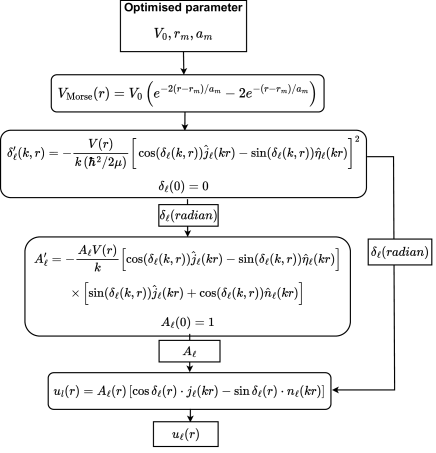
Figure 1: Detailed flowchart for obtaining phase shift, amplitude function and wavefunction.

3 Results and Discussion

Table 1: Model Parameters for Morse potential for various channels of n-p scattering [8].

States	$V_{0}(MeV)$	$r_{m}(fm)$	$a_{m}(fm)$	$MSE$
${}^{1}S_{0}$	70.438	0.901	0.372	0.649
${}^{1}P_{1}$	0.010	5.442	1.016	1.568
${}^{3}P_{0}$	11.579	1.750	0.601	0.049
${}^{3}P_{1}$	0.010	4.514	0.778	0.832
${}^{1}D_{2}$	131.302	0.010	0.526	0.026
${}^{3}D_{2}$	106.379	0.209	0.747	0.066

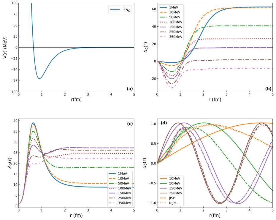
Figure 2: The potential $V(r)$, scattering phase shift $\delta(r)$, amplitude $A(r)$, and wavefunction $u(r)$ for the ${}^{1}S_{0}$ state are shown in Figure 2. The dashed line represents the potential obtained from the JISP model [18, 19], while the dotted lines correspond to the NIJM-II potential from [19].

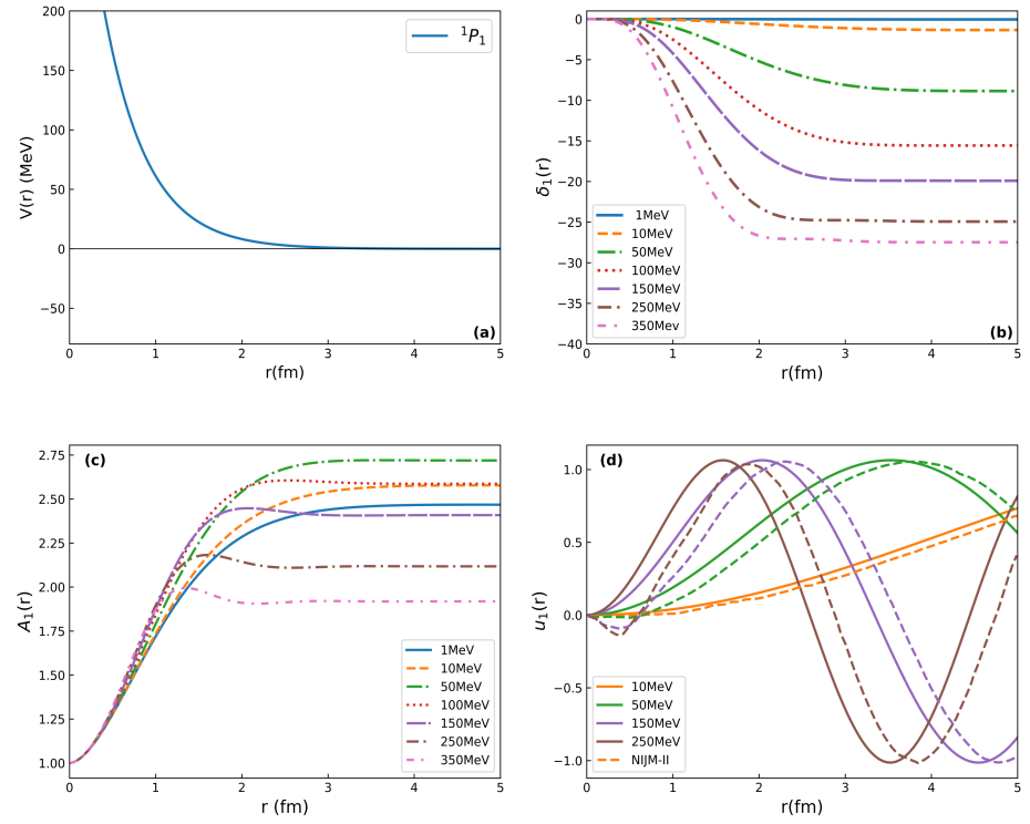
Figure 3: The potential $V(r)$, scattering phase shift $\delta(r)$, amplitude $A(r)$, and wavefunction $u(r)$ for the ${}^{1}P_{1}$ state are shown in Figure 3. The dashed lines correspond to the NIJM-II potential [19].

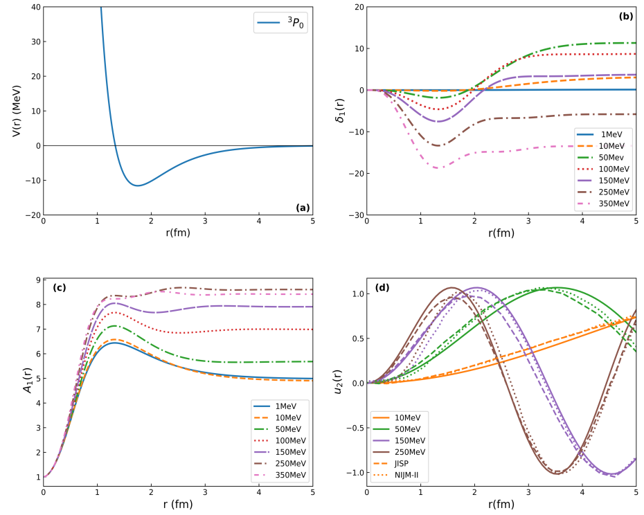
Figure 4: The potential $V(r)$, scattering phase shift $\delta(r)$, amplitude $A(r)$, and wavefunction $u(r)$ for the ${}^{3}P_{0}$ state are shown in Figure 4. The dashed line represents the potential obtained from the JISP model [18, 19], while the dotted lines correspond to the NIJM-II potential [19].

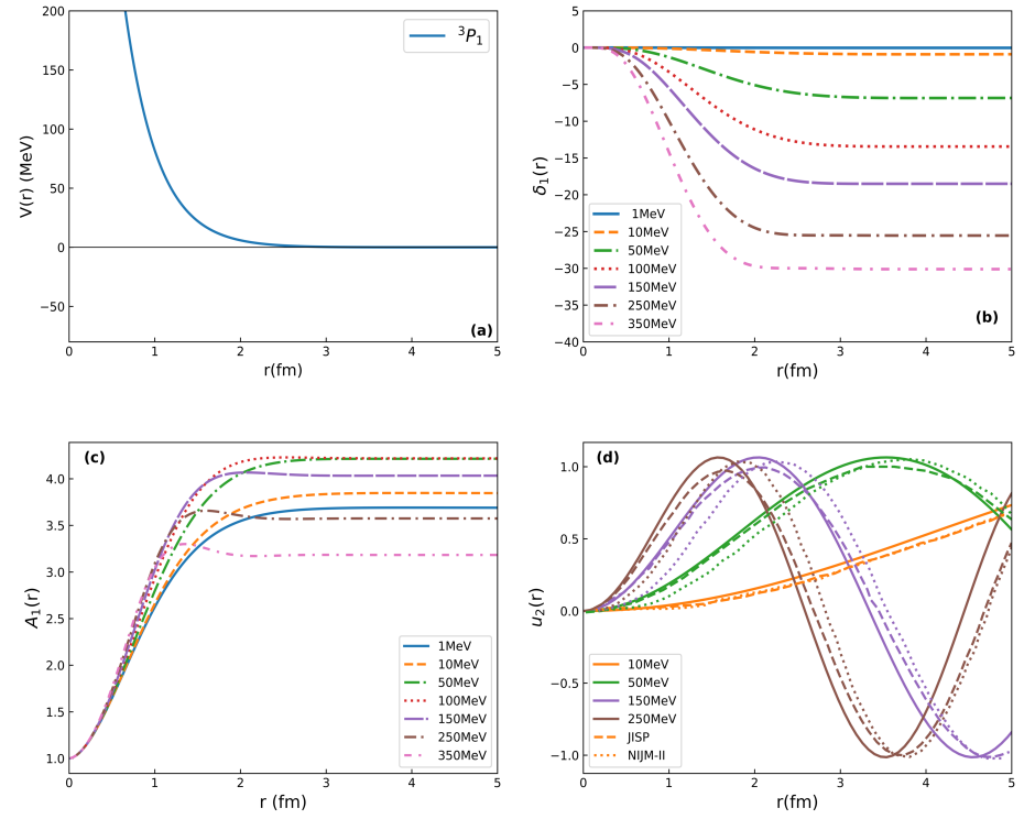
Figure 5: The potential $V(r)$, scattering phase shift $\delta(r)$, amplitude $A(r)$, and wavefunction $u(r)$ for the ${}^{3}P_{1}$ state are shown in Figure 5. The dashed line represents the potential obtained from the JISP model [18, 19], while the dotted lines correspond to the NIJM-II potential [19].

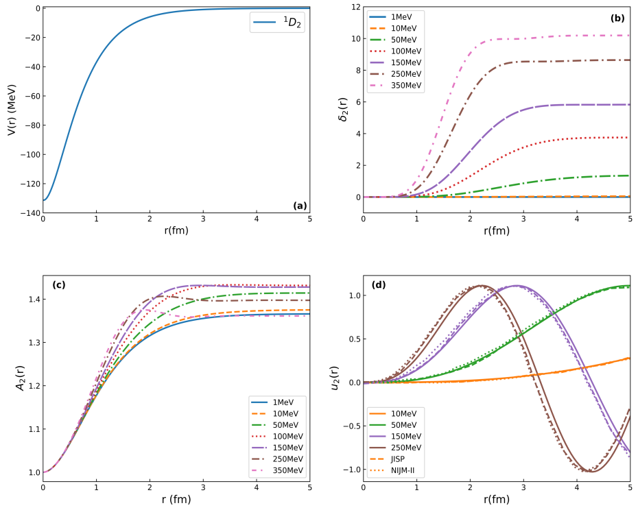
Figure 6: The potential $V(r)$, scattering phase shift $\delta(r)$, amplitude $A(r)$, and wavefunction $u(r)$ for the ${}^{1}D_{2}$ state are shown in Figure 6. The dashed line represents the potential obtained from the JISP model [18, 19], while the dotted lines correspond to the NIJM-II potential [19].

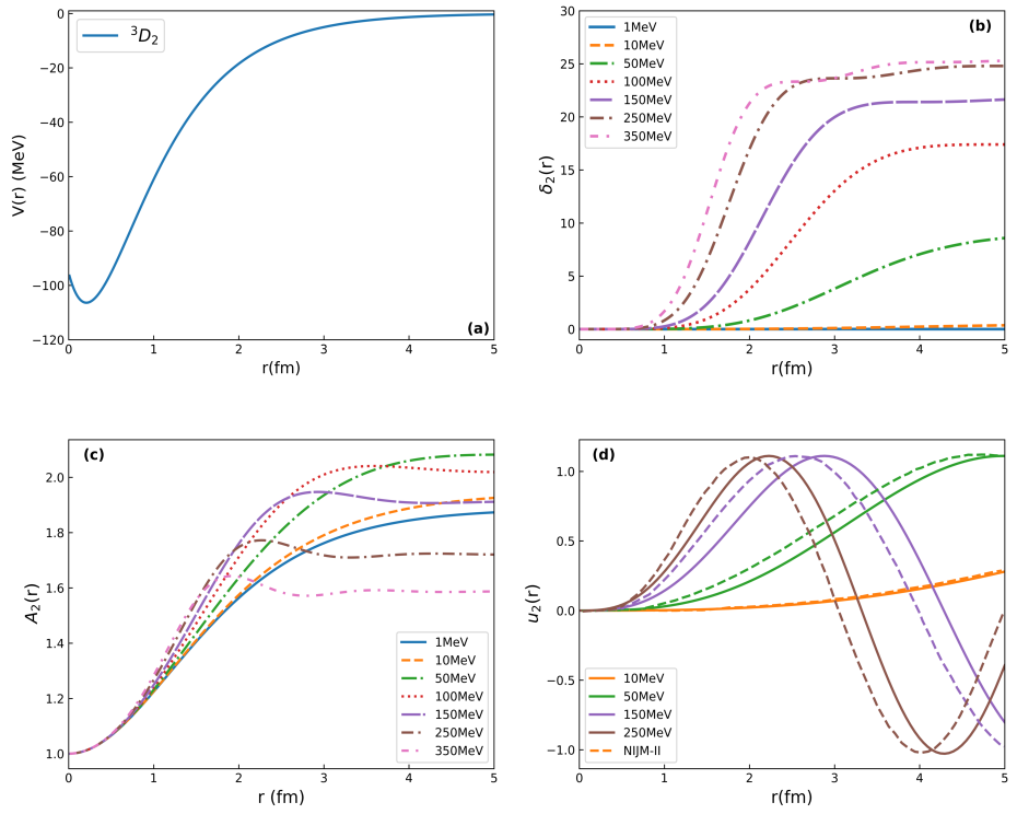
Figure 7: The potential $V(r)$, scattering phase shift $\delta(r)$, amplitude $A(r)$, and wavefunction $u(r)$ for the ${}^{3}D2$ state are shown in Figure 7. The dashed lines correspond to the NIJM-II potential [19].

3.1 Discussion

1. For ${}^{1}S_{0}$ state in the region $0\leq r\leq 1$ fm, low-energy particles face the attractive part of the potential. As the energy increases to $350$ MeV $(0\leq r\leq 1$ fm), the repulsive interaction takes place, indicating that the interaction is occurring near the repulsive core. According to the PFM equation, the repulsive potential will result in negative phase shifts. This phenomenon is clearly depicted in Figure 2(b). For $r\geq 1$ fm, the interaction moves towards the attractive core of the potential, leading to positive phase shifts. The amplitude variation for the ${}^{1}S_{0}$ state is shown in Figure2(c) and exhibits a very good match with those observed in Zhaba’s work [17] using Av-18 potential [5]. Finally, the wave functions are plotted at various energies ($E=10$, $50$, $150$, and $250$ MeV). At $10$ MeV, our obtained wave function ([14, 15] is not observed to be in good aggreement and can be seen for energies greater than $50$ MeV.

2. For ${}^{1}P_{1}$ state, the potential is purely repulsive in nature. From PFM (Phase Function Method), we know that a positive potential will lead to negative phase shifts. The variation of phase shifts can be observed to be very small for lower energies because, at lower energies, the interaction is away from the repulsive core and the effective interaction is very close to zero. However, as the energy increases, the repulsive core interaction comes into play, resulting in a significant negative phase shift. The variation of the amplitude function also exhibits reasonable variation with the NIJM-II [15].

3. ${}^{3}P_{0}$ potential is having both attractive and repulsive nature. Hence phase shift variation from negative to positive is observed in Figure 4. Almost identical variation for amplitudes at different energies is observed, which indicates that our inverse potential is in good relation with that of Av-18. A small magnitude difference between our and Zhaba’s amplitude is found, which may be a result of a small difference between the depths of Morse and Av-18 potential. Again, the wave function for the 3P0 state is found to be in very good match with those by NIJM-II [15] and JISP [14]. Our wave function can be seen to be in close agreement with those given by NIJM-II.

4. As in the ${}^{1}P_{1}$ case, for the ${}^{3}P_{1}$ state, the potential is purely repulsive in nature, as shown in Figure 5(a). From PFM, we know that a positive potential will lead to negative phase shifts, as seen in Figure 5(b). The variation of phase shifts can be observed to be very small for lower energies because, at lower energies, the interaction is away from the repulsive core and the effective interaction is very close to zero. However, as the energy increases, the repulsive core interaction comes into play, resulting in a significant negative phase shift. The variation of the amplitude function also exhibits reasonable variation with NIJM-II [15] .

5. For the ${}^{1}D_{2}$ state, the potential is having a Gaussian shape, i.e., purely attractive with a tail going to zero. This indicates that the phase shift must be purely positive, as shown in Figure 6(b). The phase shift is again in good match with that given by Zhaba. The wavefunction for the 1D2 state is in excellent agreement with that given by the Av-18 potential and JISM method, as shown in Figure 6(d).

6. For the ${}^{3}D_{2}$ state, the potential is also seen to be purely attractive. The phase shift, amplitudes, and wavefunction variation are shown in Figure 7(a), Figure 7(b), and Figure 7(c), respectively.

Overall, the results indicate that our inverse procedure is validated by obtaining the wavefunctions in close agreement with the Av-18 potential and JISP. However, a certain phase lag is observed between our results and those of NIJM-II and JISP [18, 19] for certain states. This phase lag can be attributed to the simplistic Morse model used in our approach. To refine the results, we can apply the Combinatorial Data Analysis (CDA) procedure developed by our group [4]. This procedure can generate a certain class of isospectral potentials that may provide better agreement between the compared wavefunctions in this work.

4 Conclusion

The obtained phases serve as a quantum mechanical magnification glass, allowing us to explore the intricacies of the nuclear domain. The variation of phase shift with distance provides a beautiful demonstration that, for repulsive potentials, the phase shift $\delta$ takes on positive values, while for attractive potentials, it assumes negative values. This observation aligns perfectly with the main equation of the Phase Function Method (PFM). The presence of Bessel functions in the PFM equation leads to the oscillatory nature of the phase shift for certain states. Our inverse procedure is effective in obtaining Phase shift($\delta(r)$), Amplitude($A(r)$) and Wave function($u(r)$) for various quantum mechanical states.

The wave function for specific states, such as ${}^{3}P_{0}$, ${}^{3}P_{1}$, and ${}^{1}D_{2}$, exhibits excellent agreement with those obtained by NIJM-II and JISP [18, 19]. This computational approach to constructing inverse potentials offers certain advantages, although further improvements are desired for enhanced performance. Moreover, this methodology can be extended to investigate a wide range of scattering scenarios, including $n-\alpha$, $p-\alpha$, $n-C$ among others. We are actively exploring these possibilities.

5 Acknowledgements

I am grateful to Prof. O. S. K. S. Sastri, my PhD advisor, my colleague Lalit Kumar, and M.Sc. student Sudhir Banyal for their insightful remarks and suggestions on this study.

Appendix

Amplitude Function Equations

for $\ell=0$,$\ell=1$, $\ell=2$

$$A_{0}^{\prime} =-\frac{A_{0}V(r)}{k\left(\frac{\hbar^{2}}{2\mu}\right)}\left[\cos\delta_{0}\cdot\sin(kr)-\sin\delta_{0}\cdot(-\cos(kr))\right]$$

$$\quad\times\left[\sin\delta_{0}\cdot\sin(kr)+\cos\delta_{0}\cdot(-\cos(kr))\right]$$ (12)

$$A_{1}^{\prime} =-\frac{A_{1}V(r)}{k\left(\frac{\hbar^{2}}{2\mu}\right)}\left[\cos\delta_{1}\left(\frac{\sin(kr)}{(kr)}-\cos(kr)\right)-\sin\delta_{1}\left(-\frac{\cos(kr)}{(kr)}-\sin(kr)\right)\right]$$

$$\quad\times\left[\sin\delta_{1}\left(\frac{\sin(kr)}{(kr)}-\cos(kr)\right)+\cos\delta_{1}\left(-\frac{\cos(kr)}{(kr)}-\sin(kr)\right)\right]$$ (14)

$$A_{2}^{\prime} =-\frac{A_{2}V(r)}{k\left(\frac{\hbar^{2}}{2\mu}\right)}\biggl{[}\cos\delta_{2}\left(\left(\frac{3}{(kr)^{2}}-1\right)\sin(kr)-\frac{3}{(kr)}\cos(kr)\right)$$

$$\quad\times\left(\sin\delta_{2}\left(\left(\frac{3}{(kr)^{2}}-1\right)\sin(kr)-\frac{3}{(kr)}\cos(kr)\right)+\cos\delta_{2}\left(\left(-\frac{3}{(kr)^{2}}+1\right)\cos(kr)\right.\right.$$

$$\quad\left.\left.-\frac{3}{(kr)}\sin(kr)\right)\right]$$ (15)

Wavefunction Equations

for $\ell=0$, $\ell=1$, $\ell=2$

$$u_{0}(r)=A_{0}(r)\left[\cos\delta_{0}(r)\cdot\sin(kr)-\sin\delta_{0}(r)\cdot\cos(kr)\right]$$ (16)

$$u_{1}(r)=A_{1}(r)\left[\cos\delta_{1}(r)\left(\frac{\sin(kr)}{(kr)}-\cos(kr)\right)-\sin\delta_{1}(r)\left(-\frac{\cos(kr)}{(kr)}-\sin(kr)\right)\right]$$ (17)

$$u_{2}(r)=A_{2}(r)\bigg{[}\cos\delta_{2}(r)\bigg{(}\left(\frac{3}{(kr)^{2}}-1\right)\sin(kr)-\frac{3}{(kr)}\cos(kr)\bigg{)}$$

$$\qquad-\sin\delta_{2}(r)\bigg{(}-\left(-\frac{3}{(kr)^{2}}+1\right)\cos(kr)-\frac{3}{(kr)}\sin(kr)\bigg{)}\bigg{]}$$ (18)

References

- [1] Blatt, J.M. and Jackson, J.D., 1949. On the interpretation of neutron-proton scattering data by the Schwinger variational method. Physical Review, 76(1), p.18.
- [2] Khachi, A., Kumar, L. and Sastri, O.S.K.S., 2021. Neutron-Proton Scattering Phase Shifts in S-Channel using Phase Function Method for Various Two Term Potentials. Journal of Nuclear Physics, Material Sciences, Radiation and Applications, 9(1), pp.87-93.
- [3] Sastri, O.S.K.S., Khachi, A. and Kumar, L., 2022. An Innovative Approach to Construct Inverse Potentials Using Variational Monte-Carlo and Phase Function Method: Application to np and pp Scattering. Brazilian Journal of Physics, 52(2), p.58.
- [4] Khachi, A., Kumar, L., Kumar, M.G. and Sastri, O.S.K.S., 2023. Deuteron structure and form factors: Using an inverse potential approach. Physical Review C, 107(6), p.064002.
- [5] Awasthi S., Sastri O. S. K. S., 2023. Real and Imaginary Phase Shifts for Nucleon-Deuteron Scattering using Phase Function Method. arXiv:2304.10478
- [6] Kumar, L., Khachi, A. and Sastri, O.S.K.S., 2022. Phase Shift Analysis for Neutron-Alpha Elastic Scattering Using Phase Function Method with Local Gaussian Potential. Journal of Nuclear Physics, Material Sciences, Radiation and Applications, 9(2), pp.215-221.
- [7] Morse, P.M., 1929. Diatomic molecules according to the wave mechanics. II. Vibrational levels. Physical review, 34(1), p.57.
- [8] Khachi, A., Kumar, L., Awasthi, A. and Sastri, O.S.K.S., 2023. Inverse potentials for all channels of neutron-proton scattering using reference potential approach. Physica Scripta, 98, 095301
- [9] Khirali, B., Behera, A.K., Bhoi, J. and Laha, U., 2020. Scattering with Manning–Rosen potential in all partial waves. Annals of Physics, 412, p.168044.
- [10] Malfliet, R.A. and Tjon, J.A., 1969. Solution of the Faddeev equations for the triton problem using local two-particle interactions. Nuclear Physics A, 127(1), pp.161-168.
- [11] Bhoi, J. and Laha, U., 2017. Hulthen potential models for and elastic scattering. Pramana, 88, pp.1-6.
- [12] F. Calogero, Variable Phase Approach to Potential Scattering (Academic, New York, 1967)
- [13] Babikov, V.V.E., 1967. The phase-function method in quantum mechanics. Soviet Physics Uspekhi, 10(3), p.271.
- [14] Butcher, J.C., 1996. A history of Runge-Kutta methods. Applied numerical mathematics, 20(3), pp.247-260.
- [15] Morse, P.M. and Allis, W.P., 1933. The effect of exchange on the scattering of slow electrons from atoms. Physical Review, 44(4), p.269.
- [16] Palov, A.P. and Balint-Kurti, G.G., 2021. VPA: computer program for the computation of the phase shift in atom–atom potential scattering using the variable phase approach. Computer Physics Communications, 263, p.107895.
- [17] Zhaba, V.I., 2019. The variable phase approach: phase, amplitude and wave functions of the states for np-system for Argonne v18 potential. World Scientific News, (123), pp.161-180.
- [18] Mazur, A.I., Shirokov, A.M., Vary, J.P., Weber, T.A., Zaitsev, S.A. and Mazur, E.A., 2007. Nonlocal nucleon-nucleon interaction JISP. Bulletin of the Russian Academy of Sciences: Physics, 71, pp.754-763.
- [19] Shirokov, A.M., Mazur, A.I., Zaytsev, S.A., Vary, J.P. and Weber, T.A., 2004. Nucleon-nucleon interaction in the J-matrix inverse scattering approach and few-nucleon systems. Physical Review C, 70(4), p.044005.