Parametric Modeling of Serpentine Waveguide Traveling Wave Tubes

Abstract

A simple and fast model for numerically calculating small-signal gain in serpentine waveguide traveling-wave tubes (TWTs) is described. In the framework of the Pierce model, we consider one-dimensional electron flow along a dispersive single-mode slow-wave structure (SWS), accounting for the space-charge effect. The analytical model accounts for the frequency-dependent phase velocity and characteristic impedance obtained using various equivalent circuit models from the literature, validated by comparison with full-wave eigenmode simulation. The model includes a relation between the modal characteristic impedance and the interaction (Pierce) impedance of the SWS, including also an extra correction factor that accounts for the variation of the electric field distribution and hence of the interaction impedance over the beam cross section. By applying boundary conditions to our generalized Pierce model, we compute both the theoretical gain of a TWT and all the complex-valued wavenumbers of the hot modes versus frequency and compare our results with numerically intensive particle-in-cell (PIC) simulations; the good agreement in the comparison demonstrates the accuracy and simplicity of our generalized model. For various examples where we vary the average electron beam (e-beam) phase velocity, average e-beam current, number of unit cells, and input radio frequency (RF) power, we demonstrate that our model is robust in the small-signal regime.

I Introduction

The traveling-wave tube (TWT) is a type of common microwave vacuum electron tube that has been widely used for applications such as communication, radar, and electronic countermeasures [1, 2, 3]. Among the different kinds of TWTs, the serpentine waveguide TWT has advantages over other kinds of millimeter wave TWTs (e.g. helix TWT, coupled cavity (CC) TWT, ring-bar TWT) due to its moderate bandwidth with power-handling capacity at higher frequencies and its compatibility with planar fabrication using lithography or micromachining [4, 5, 6, 7, 8]. The slow-wave structure (SWS) of the serpentine waveguide TWT is formed by bending rectangular waveguides in the electric field plane ($E$-plane). Also, a cylindrical electron beam (e-beam) is transported through the cylindrical beam tunnel to interact with the radio frequency (RF) propagating wave. Although the serpentine waveguide SWS’s performance is limited by its low interaction impedance and interaction efficiency, many schemes of enhancing the on-axis interaction impedance and also enhancement of interaction efficiency have been proposed [9, 10, 11, 12, 13, 14].

In order to analyze the e-beam and electromagnetic (EM) wave dynamics of a serpentine waveguide TWT, it is necessary to examine the EM characteristics of the SWS. Various analytical models have been developed for its characterization. In 1987, Dohler et al. proposed a simple analytical method for determining the dispersion characteristics and the interaction impedance of the EM modes in the serpentine waveguide [4]. Liu suggested an analytical formulation adding the effect of bends [5]. Then, researchers developed a closed-form algebraic dispersion relation based on an equivalent circuit model that also considered the effect of mismatch between straight and bend sections as well as an approximate model for beam holes [15, 16]. A thorough equivalent circuit analysis of serpentine waveguides by modeling the effect of beam tunnels as orthogonal stubs was developed by Booske et al. [17] for the calculation of dispersion characteristics, following the approach of transmission line (TL) cascading networks and benchmarked using three-dimensional (3D) simulations with Ansys HFSS, MAFIA, and CST Studio Suite. Recently, Antonsen et al. [18] developed a hybrid model consisting of a combination of TL segments and lumped electrical elements, which is utilized to analyze serpentine waveguide dispersion characteristics and interaction impedance. The model also captures the effects of asymmetric fields and beam tunnel misalignment. Although some commercial full-wave simulation software like Ansys HFSS and CST Studio Suite are versatile and can analyze SWS characteristics, simulation times are longer than analytical methods. Therefore, analytical methods are preferred for quickly iterating through and optimizing various SWS designs.

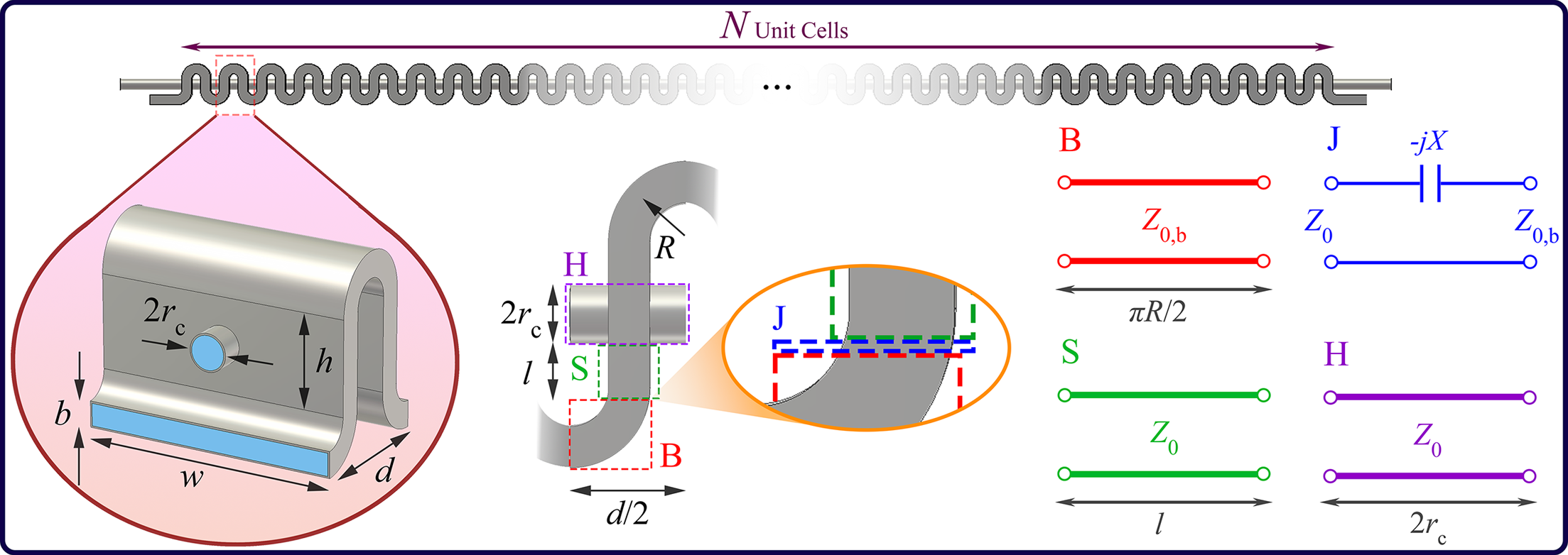
Figure 1: Schematic illustration of a serpentine waveguide unit cell, constitutive segments (colored dashed rectangles), and parametric dimensions are shown in the left and central panels. The equivalent TL model for the TE10 mode in each segment is shown in the right panel for: (B) $E$-plane circular bend, (J) circular bend to straight waveguide junction, (S) straight waveguide section, and (H) e-beam hole.

To design and analyze serpentine waveguide TWTs, various beam-EM wave interaction models exist. Particle-in-cell (PIC) simulation has been widely used to characterize the beam-EM wave interaction of TWTs because it is capable of predicting amplification performance more accurately than cold-circuit simulations alone. Nevertheless, the computational burden of 3D PIC simulators is high compared to other TWT codes. The United States Naval Research Laboratory applied the hybrid TL model to the large signal beam-EM wave interaction programs (CHRISTINE-CC and TESLA-CC), which are used for analyzing CC-TWTs. Then, they extended a 1D frequency-domain interaction model named CHRISTINE-FW developed for folded waveguide TWTs [19] and a two-dimensional (2D) frequency-domain interaction model named TESLA-FW [20, 21]. Also, a large signal beam-EM wave interaction code with computation time improvement was developed by Meyne et al. [22]. A 3D steady-state beam-EM wave interaction code using a three-port network representation of the circuit and a set of discrete ray representations of the 3D e-beam was developed by Yan et al. [23]. In addition to previous models, a nonlinear model for the numerical simulation of terahertz serpentine waveguide TWT is described in [24] in which the propagated EM wave in the SWS is represented as an infinite set of space harmonics that interact with an e-beam. Also, an improved large-signal model was developed in [25], which predicts beam-EM wave interaction with an analytical method. Recently, Figotin [26] advanced a Lagrangian field theory of CC-TWTs that integrates into it the space-charge effects; that model can also be used for serpentine waveguide TWTs as explained in detail in that paper.

In this paper, we present an analytical model for analyzing beam-EM wave interactions in serpentine waveguide TWTs shown in Fig. 1. We develop a model that can be used to obtain the small-signal gain and the "hot eigenmodes" dispersion, accounting for nonuniform beam-EM wave interaction. Hot eigenmodes exist in a TWT when the e-beam interacts with the guided EM wave. First, we show various methods from the literature that can be used to calculate SWS cold characteristics, i.e., characteristic impedance and phase velocity, based on the equivalent circuit model presented in [17]. We calculate the interaction impedance, which is one of the critical parameters for predicting TWT gain. Based on the fundamental equations of the Pierce model [27, 28, 29, 30], we further develop the model to account for frequency-dependent parameters and the space-charge effect, following the method explained in [31] for a helix TWT. Then, we introduce the frequency-dependent coupling strength coefficient which shows the strength of the interaction between e-beam and EM wave and also connects interaction impedance and characteristic impedance. We also include the small frequency-independent factor $\delta_{\mathrm{e}}$ that corrects for the nonuniform interaction impedance over the beam cross section. This correction factor models the nonuniform interaction between the EM wave and the e-beam in the interaction gap. Moreover, we model the e-beam effect on the equivalent TL model by using the electronic beam admittance per unit length $Y_{\mathrm{b}}$, accounting for the space-charge effect. By introducing $Y_{\mathrm{b}}$, it is possible to find out the conditions that lead to amplification in the TWT system. Finally, we utilize the proposed theoretical method to predict the gain versus frequency of a TWT amplifier and we compare our results to those from numerically intensive 3D PIC simulations, showing high accuracy. In order to show the flexibility and accuracy of our method, comparison with 3D PIC simulations for many examples is done by varying the e-beam parameters such as the average e-beam phase velocity, average e-beam current, number of unit cells, and input RF power.

The organization of this paper is as follows. In Section II, we highlight the main achievements of our developed model. Then, we show how to combine some analytical methods from the literature to calculate the cold parameters of the serpentine waveguide in Section III. An example of a cold model characteristic calculation is presented in Section IV. We describe the conventional method to calculate interaction impedance and introduce the extra correction factor required for our model in Section V. We develop a model for beam-EM wave interaction in Section VI and evaluate it by providing an example in Section VII, where we apply boundary conditions to determine the TWT gain. Next, we demonstrate the accuracy and efficiency of our model in Section VIII by varying TWT parameters. Finally, we conclude the paper in Section IX and discuss the supplementary information in the Appendices.

II Summary of Main Results

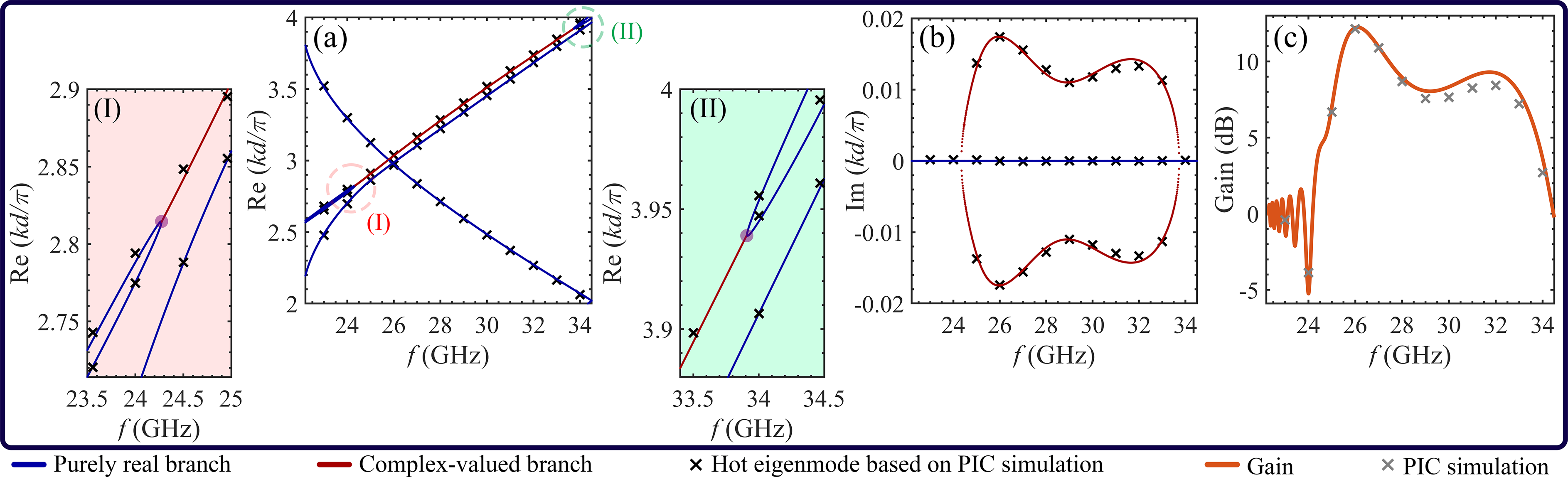
Figure 2: The (a) real and (b) imaginary parts of complex-valued wavenumbers of the hot modes, where dark blue curves indicate branches with purely real wavenumbers, dark red curves indicate branches with complex-valued wavenumbers, and black crosses indicate the results obtained using a hot eigenmode solver for beam-loaded SWS based on PIC simulations [32]. (I) and (II) show the real part of the complex-valued wavenumbers of the hot modes near the two transition points (purple circles). (c) The theoretical and PIC simulated gain versus frequency are depicted in orange curves and gray crosses, respectively. The parameters used for this example are provided in Sections IV and VII.

We present a summary of the main results calculated by our developed model and compared to PIC simulations, leaving explanations, technical details and numerical examples in the sections that follow. Figures 2(a) and (b) illustrate the real and imaginary parts of complex-valued wavenumbers of the eigenmodes supported by the serpentine waveguide with the e-beam, i.e., of the hot modes, for the example with the parameters provided in Sections IV and VII. The solid lines in Figs. 2(a) and (b) represent the calculated frequency dispersion of the hot modes resulting from the interaction between the guided EM wave in the SWS and the two space charge waves of the e-beam. The dark blue curves indicate “stable branches” whose imaginary parts of the wavenumber of the hot modes are equal to zero and hence are not amplified. In contrast, dark red curves indicate branches whose imaginary parts of the wavenumber are nonzero, and the positive values of the imaginary part allow for amplification (unstable or amplification branch). In order to verify our theoretical calculations displayed by solid curves, we calculate the real and imaginary parts of the complex-valued wavenumbers of the hot modes at a discrete set of frequencies by using the “hot eigenmode solver” for beam-loaded SWS based on PIC simulations developed in [32] (indicated by black crosses). There is excellent agreement between our theoretical model and the PIC-based model of [32], both in the real and imaginary parts of the complex wavenumber. In addition, we show the zoomed-in plot of the real part of the complex-valued wavenumber near the two transition points (bifurcations) in Figs. 2(I) and (II). The purple circles indicate the transition points that separate the stable branches with purely real wavenumbers from the unstable branches with complex-valued wavenumbers. Some features of these critical points have been previously explored in [31, 33]. Lastly, we calculate the gain versus frequency diagram for the TWT using the developed theoretical model, shown by the solid orange curve in Fig. 2(c), and compare with results from computationally intensive 3D PIC simulations, shown by gray crosses, demonstrating very good agreement. The camel-like hump curve on the gain diagram in Fig. 2(c) has the same shape as the unstable branch in Fig. 2(b). The excellent agreement between our developed theoretical results and PIC simulated results in Fig. 2 demonstrates the accuracy of our method.

III Equivalent Circuit Model of Cold SWS

It is crucial to have a simple model that estimates the cold (i.e., without the e-beam) characteristics of the SWS, especially for evaluating the operational bandwidth and interaction efficiency of TWTs. Here, we present the cold equivalent circuit model and compare frequency-dependent cold results, such as phase velocity, with those of full-wave eigenmode simulations.

A schematic design of an $E$-plane bend serpentine waveguide circuit is shown in Fig. 1. It is assumed that only the fundamental transverse-electric (TE) mode, i.e., TE10, propagates along the waveguide with a rectangular cross section. In practice, reflections at the junction with a bend cannot be completely avoided (segment J), and we also need to take into account that the characteristic impedance of the EM mode in the bend (segment B) is slightly different from that of the EM mode in the straight segment; hence, the junction between the two segments involves reactive fields [34, 35, Ch. 4]. Note that the U-shaped bends in serpentine waveguides considered here produce less reflection than the right angle bends commonly found in folded waveguides [16, 36, 37]. Additionally, reactive loading from the beam hole (segment H) can affect device performance, depending on the hole’s diameter. The effect of both of these kinds of reflections is the creation of a stopband that may limit the TWT’s maximum operating frequency. In addition, a band edge can also be a source of instability if an e-beam synchronizes with it [16, 38]. The different segments of the serpentine waveguide are represented in the center panel of Fig. 1, each with its own equivalent TL circuit in the right panel. In this case, B, J, S, and H correspond to the following parts of the unit cell: $E$-plane circular bend, circular bend to straight waveguide junction, straight waveguide section, and e-beam hole, respectively. By multiplying (cascading) the transfer matrices of the individual segments we build the equivalent TL model corresponding to the serpentine waveguide’s unit cell which will be further discussed in Subsection III-B. The equivalent voltage and current in the TLs are calculated at discrete locations using the transfer matrix $\mathbf{\underline{T}}_{\mathrm{U}}$ as

$$\boldsymbol{\Psi}_{n}=\left[\begin{array}[]{c}V_{n}\\ I_{n}\end{array}\right],\;\boldsymbol{\Psi}_{n}=\mathbf{\underline{T}}_{\mathrm{U}}\boldsymbol{\Psi}_{n-1},$$ (1)

where $V_{n-1}$ and $I_{n-1}$ are the equivalent voltage and current [34] at the input port of the $n$th unit cell and $V_{n}$ and $I_{n}$ are the equivalent voltage and current at the output port of the $n$th unit cell as shown in Fig. 3. See also Appendix A for more details.

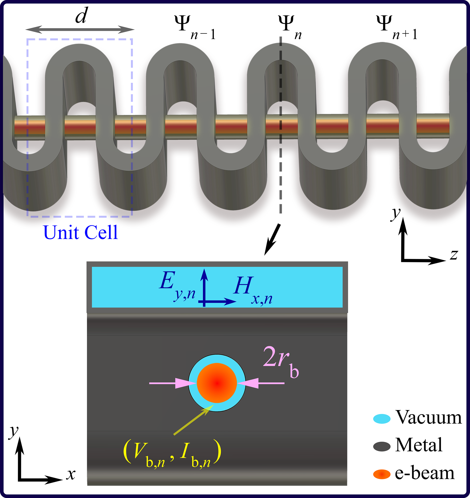
Figure 3: Equivalent voltage and current at the input and output of each unit cell and the corresponding TE10 electric and magnetic fields in the cross section of the serpentine waveguide. We also show the equivalent kinetic beam voltage and beam current pertinent to the two charge waves.

III-A Equivalent Matrix for Each Segment

III-A1 Straight Waveguide (Segment S)

The straight rectangular waveguide segment of the unit cell is modeled as a uniform TL of length $l$ with characteristic modal impedance $Z_{0}=\eta_{0}/\sqrt{1-\left(\omega_{\mathrm{co}}/\omega\right)^{2}}$ of the fundamental TE10 mode, where $\eta_{0}=\sqrt{\mu_{0}/\varepsilon_{0}}$ is the wave impedance of free space, $\omega_{\mathrm{co}}=\pi c/w$ is the cutoff angular frequency, $w$ is the width of the rectangular waveguide, and $\omega$ is the operating angular frequency. The phase propagation constant of the TE10 mode is $\beta_{\mathrm{g,s}}=\sqrt{k_{0}^{2}-\left(\pi/w\right)}$, where $k_{0}=2\pi/\lambda_{0}$, and $\lambda_{0}=2\pi c/\omega$ is wavelength in free space. The equivalent TL circuit representation of the straight waveguide segment is shown in Fig. 1 (segment S), and the equivalent transfer matrix is

$$\mathbf{\underline{T}}_{\mathrm{S}}=\left[\begin{array}[]{rr}\cos\left(\beta_{\mathrm{g,s}}l\right)&jZ_{0}\sin\left(\beta_{\mathrm{g,s}}l\right)\\ j\sin\left(\beta_{\mathrm{g,s}}l\right)/Z_{0}&\cos\left(\beta_{\mathrm{g,s}}l\right)\end{array}\right].$$ (2)

III-A2 Circular Bend to Straight Waveguide Junction (Segment J)

The junction between the straight waveguide and the $E$-plane bend is represented by the equivalent circuit in Fig. 1 (segment J) with equivalent lumped reactance [34, Sec. 5.34]

$$X=Z_{0}\left(\frac{32}{\pi^{7}}\left(\frac{2\pi b}{\lambda_{\mathrm{g,s}}}\right)^{3}\left(\frac{b}{R}\right)^{2}\sum_{n=1,3,\ldots}^{\infty}\frac{1}{n^{7}}\sqrt{1-\left(\frac{2b}{n\lambda_{\mathrm{g,s}}}\right)^{2}}\right),$$ (3)

where $R$ is the mean radius of the bend, and $\lambda_{\mathrm{g,s}}=2\pi/\beta_{\mathrm{g,s}}=\lambda_{0}/\sqrt{1-\left(\omega_{\mathrm{co}}/\omega\right)^{2}}$ is the guided wavelength. The equivalent transfer matrix for the junction is

$$\mathbf{\underline{T}}_{\mathrm{J}}=\left[\begin{array}[]{rr}1&-jX\\ 0&1\end{array}\right].$$ (4)

III-A3 $E$-plane Circular Bend (Segment B)

An equivalent TL circuit for the quarter $E$-plane bend is given in Fig. 1 (segment B). Here, $\pi R/2$ is the mean length of the $E$-plane bend and the length of the equivalent TL. The modified characteristic impedance for the fundamental propagating mode in the bend is [34, Sec. 5.34]

$$Z_{0,\mathrm{b}}=Z_{0}\left(1+\frac{1}{12}\left(\frac{b}{R}\right)^{2}\left[\frac{1}{2}-\frac{1}{5}\left(\frac{2\pi b}{\lambda_{\mathrm{g,s}}}\right)^{2}\right]\right).$$ (5)

In addition, the circular bend is considered as a uniform angular waveguide with a guided wavelength of

$$\lambda_{\mathrm{g,b}}\simeq\lambda_{\mathrm{g,s}}\left(1-\frac{1}{12}\left(\frac{b}{R}\right)^{2}\left[-\frac{1}{2}+\frac{1}{5}\left(\frac{2\pi b}{\lambda_{\mathrm{g,s}}}\right)^{2}-\ldots\right]\right),$$ (6)

for the fundamental mode. As a result, in the wavelength range $2b/\lambda_{\mathrm{g,s}}<1$ [34, Sec. 5.34], the TL matrix for the circular bend segment is

$$\mathbf{\underline{T}}_{\mathrm{B}}=\left[\begin{array}[]{rr}\cos\left(\frac{\pi^{2}R}{\lambda_{\mathrm{g,b}}}\right)&jZ_{0,\mathrm{b}}\sin\left(\frac{\pi^{2}R}{\lambda_{\mathrm{g,b}}}\right)\\ j\sin\left(\frac{\pi^{2}R}{\lambda_{\mathrm{g,b}}}\right)/Z_{0,\mathrm{b}}&\cos\left(\frac{\pi^{2}R}{\lambda_{\mathrm{g,b}}}\right)\end{array}\right].$$ (7)

III-A4 Beam Tunnel Hole

The radius of the beam hole can slightly affect the phase velocity, dispersion and cutoff frequency of the EM mode in the SWS [39, 40]. A wide beam tunnel will add significant periodic reactive loading to the SWS and introduce a stopband at the $3\pi$ point of the modal dispersion diagram, and the larger beam tunnel radius results in a larger stopband [41]. On the other hand, a wide beam tunnel permits higher beam currents since the beam radius can be larger with the same current density, resulting in higher d.c. beam power and output RF power at saturation [42]. However, an e-beam of a very small radius (with the same d.c. beam current) will experience strong Coulomb repulsion between electrons, and it is unrealistic to apply an intense magnetic field to confine an e-beam with a small radius and high current density [41]. Also, it is desirable to have an e-beam with a lower accelerating voltage and a higher current, resulting in a higher gain. Therefore, it is necessary to trade off beam tunnel size, current density, and beam radius to optimize TWT properties, such as linear gain and efficiency.

A general and accurate circuit to model the beam tunnel hole that can be used in all cases has not been developed yet. In [15], the authors modeled the circular hole as a shunt reactance, where the value depends on rectangular waveguide width and height and beam tunnel diameter. Also, in [17], a circuit model of the beam tunnel hole based on the modification of the model for different tunnel radii in [34] was presented. The reference structure is a circular waveguide connected orthogonally to the broad wall of a rectangular waveguide through a small aperture. The difference between the reference structure in [34] and the structure to be modeled is that the cylindrical tunnel is represented as a stub whose diameter equals the aperture diameter and is below the cutoff for propagation and there are two of these stubs present. By assuming that the hole radius is electrically small (i.e., much smaller than the guided wavelength), we can often neglect the effect of holes and model this section as a simple straight rectangular waveguide as we described in Subsection III-A1. This approximation leads to acceptable results and more investigation for an specific example is provided in Appendix B.

III-B Cascaded Circuit Model

The basic SWS segments shown in Fig. 1 are represented by equivalent TL segments, each with an equivalent transfer matrix as discussed above. The transfer matrices for the lossless circuit segments are cascaded to arrive at the transfer matrix of the unit cell represented as

$$\begin{array}[]{c}\mathbf{\underline{T}}_{\mathrm{U}}=\left[\begin{array}[]{cc}T_{11}&T_{12}\\ T_{21}&T_{22}\end{array}\right]=\left(\mathbf{\underline{T}}_{\mathrm{U/2}}\right)^{2}.\end{array}$$ (8)

For convenience we use the half unit cell transfer matrix defined as

$$\mathbf{\underline{T}}_{\mathrm{U/2}}=\left(\mathbf{\underline{T}}_{\mathrm{B}}\mathbf{\underline{T}}_{\mathrm{J}}\mathbf{\underline{T}}_{\mathrm{S}}\mathbf{\underline{T}}_{\mathrm{H}}\mathbf{\underline{T}}_{\mathrm{S}}\mathbf{\underline{T}}_{\mathrm{J}}\mathbf{\underline{T}}_{\mathrm{B}}\right).$$ (9)

Using our unit cell transfer matrix $\mathbf{\underline{T}}_{\mathrm{U}}$, we find solutions for the state vector, $\boldsymbol{\Psi}=\left[V,I\right]^{\mathrm{T}}$, that satisfies

$$\mathbf{\underline{T}}_{\mathrm{U}}\boldsymbol{\Psi}=e^{-\mathit{j}\beta_{\mathrm{c,0}}\mathit{d}}\boldsymbol{\Psi},$$ (10)

where $d$ is unit cell period and $\mathit{\beta_{\mathrm{c,0}}}$ is the wavenumber of the fundamental spatial harmonic. Solving the eigenvalue problem,

$$\mathrm{det\left(\mathbf{\underline{T}}_{\mathrm{U}}-e^{-\mathit{j}\mathit{\beta_{\mathrm{c,0}}}\mathit{d}}\mathbf{\underline{I}}\right)}=0,$$ (11)

for $\beta_{\mathrm{c,0}}$, yields the Bloch wavenumbers of the cold EM modes allowed in the SWS, where $\mathbf{\underline{I}}$ is the $2\times 2$ identity matrix. Then, the propagation constants for the $m$th spatial harmonic is

$$\beta_{\mathrm{c},m}=\beta_{\mathrm{c,0}}+\frac{2m\pi}{d},\quad m=0,\pm 1,\pm 2,\ldots$$ (12)

The phase velocity of the spatial harmonic of the cold mode is calculated as $v_{\mathrm{c},m}=\omega/\beta_{\mathrm{c},m}$. Based on the definition of the state vector at the beginning of each unit cell, the characteristic Bloch impedance of the fundamental guided mode is calculated as

$$Z_{\mathrm{c}}=\frac{V}{I}=\frac{\left(T_{22}-e^{-\mathit{j}\beta_{\mathrm{c},0}\mathit{d}}\right)}{T_{21}}=\frac{T_{12}}{\left(T_{11}-e^{-\mathit{j}\beta_{\mathrm{c},0}\mathit{d}}\right)}.$$ (13)

Note that the Bloch impedance depends on where the section separating unit cells is defined, and if we substitute $\beta_{\mathrm{c},0}$ for $\beta_{\mathrm{c},m}$, the result does not change.

III-C Equivalent Uniform TL Model

Each EM mode is comprised of a fundamental Bloch wavenumber $\beta_{\mathrm{c,0}}$ and all its spatial harmonics $\beta_{\mathrm{c},m}$. However, the Pierce model [27, 29, 30] is based on the assumption that the SWS can be considered as a uniform TL supporting a single mode with wavenumber $\beta_{\mathrm{c}}$ that is velocity-synchronized with the e-beam, which is discussed here. To highlight this view, we impose that the cascaded matrix $\mathbf{\underline{T}}_{\mathrm{U}}$ in (8) should be equal to the transfer matrix of an equivalent uniform single TL, as was done also in [15, 17],

$$\begin{array}[]{c}\mathbf{\underline{T}}_{\mathrm{Uni}}=\left[\begin{array}[]{rr}\cos\left(\beta_{\mathrm{c,0}}d\right)&jZ_{\mathrm{c}}\sin\left(\beta_{\mathrm{c,0}}d\right)\\ j\sin\left(\beta_{\mathrm{c,0}}d\right)/Z_{\mathrm{c}}&\cos\left(\beta_{\mathrm{c,0}}d\right)\end{array}\right]\\ =\left[\begin{array}[]{rr}T_{\mathrm{a}}&T_{\mathrm{b}}\\ T_{\mathrm{c}}&T_{\mathrm{a}}\end{array}\right]\equiv\left(\mathbf{\underline{T}}_{\mathrm{U/2}}\right)^{2}.\end{array}$$ (14)

Since the right-hand side of (14) is calculated from the circuit equivalent model of each segment as explained in the previous subsection, we obtain the elements of $\mathbf{\underline{T}}_{\mathrm{Uni}}$ for $\beta_{\mathrm{c,0}}d$, which is the effective phase shift per unit cell of the fundamental spatial harmonic. As a result, the propagation constants for all spatial harmonics are [43, Sec. 4.5.1]

$$\beta_{\mathrm{c},m}=\frac{\cos^{-1}\left(T_{\mathrm{a}}\right)}{d}+\frac{2m\pi}{d},\quad m=0,\pm 1,\pm 2,\ldots,$$ (15)

where $m$ denotes the harmonic number. In serpentine waveguide TWTs usually the first spatial harmonic ($m=1$) is synchronized with the e-beam. The phase velocity corresponding to the $m$th spatial harmonic is $v_{\mathrm{c},m}=\omega/\beta_{\mathrm{c},m}$. The second and third elements in the equivalent transmission matrix $\mathbf{\underline{T}}_{\mathrm{Uni}}$ are used to calculate the modal characteristic impedance of the equivalent uniform TL as $Z_{\mathrm{c}}=\sqrt{T_{\mathrm{b}}/T_{\mathrm{c}}}$ [43, Sec. 4.5.1].

III-D Waveguide Projection Model (Without Considering the Junction and Bend Effect)

The guided wavenumbers $\beta_{\mathrm{c},m}$ can also be approximated by considering the SWS as a straightened version of the serpentine waveguide. In this simple view, the effect of the junction between straight and bend sections is ignored and we assume that the TE10 propagation constant in the curved segments is the same as in the straight segments. The on-axis phase shift per pitch for the $m$th spatial harmonics is $\beta_{\mathrm{c},m}d=\theta+2m\pi$, where $\beta_{\mathrm{c},m}$ is the effective on-axis propagation constant, $\theta=\beta_{\mathrm{g,s}}L$ is phase delay per pitch of EM wave, and $L=2\left(\pi R+h\right)$ is defined as the distance traveled by the wave per pitch. The phase velocity of $m$th spatial harmonics is expressed by [44]

$$v_{\mathrm{c},m}=\frac{\omega}{\beta_{\mathrm{c},m}}=\frac{\omega d}{\beta_{\mathrm{g,s}}L+2\pi m}.$$ (16)

The derivation of (16) assumes that the bends do not present significant mismatches to the wave. In practice, both the bends and the beam holes introduce small mismatches that may cause stopbands where the dispersion curves of spatial harmonics cross. These effects are ignored in this simplified model.

IV Validation of Equivalent Circuit Model

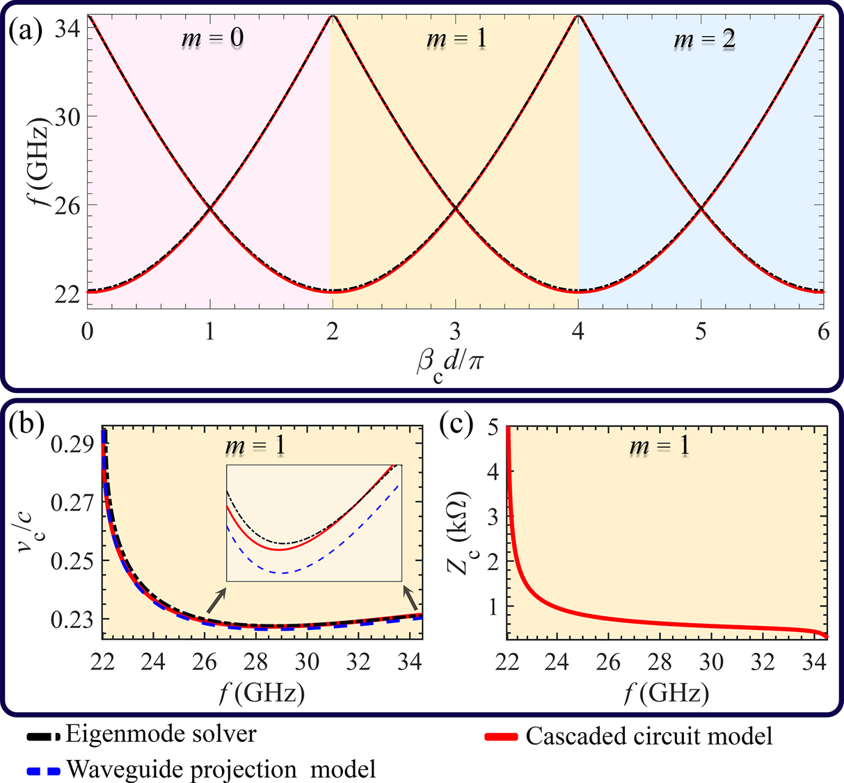
Figure 4: Cold simulation results for the serpentine waveguide using theoretical and simulation methods. (a) Modal dispersion curves for three spatial harmonics ($m=0,1$ and $2$) by employing the full-wave eigenmode solver (dashed black curves) and cascaded circuit model (solid red curve). (b) Normalized phase velocity for the first spatial harmonic ($m=1$) by using the eigenmode solver (dashed black curves), cascaded circuit model (solid red curve) and waveguide projection model (dashed blue curves). Also, the zoomed-in version of normalized phase velocity in the frequency range from $26\>\mathrm{GHz}$ to $34.5\>\mathrm{GHz}$ is shown to demonstrate the superior accuracy of the cascaded circuit model compared to the waveguide projection model. (c) Characteristic impedance for the first spatial harmonic ($m=1$) calculated using a cascaded circuit model (solid red curve).

The cold SWS characteristics for a specific design are shown via the three theoretical models discussed in the previous section, compared with simulations performed using the CST Studio Suite eigenmode solver. Figure 1 shows the model of a typical serpentine waveguide with a cylindrical beam tunnel, where the geometric parameters $w$, $b$, $d$, $h$, and $r_{\mathrm{c}}$ represent the dimensions of wide side, narrow side, full period, straight waveguide wall, and radius of beam tunnel, respectively. The parameter values for a specific design are listed in Table I.

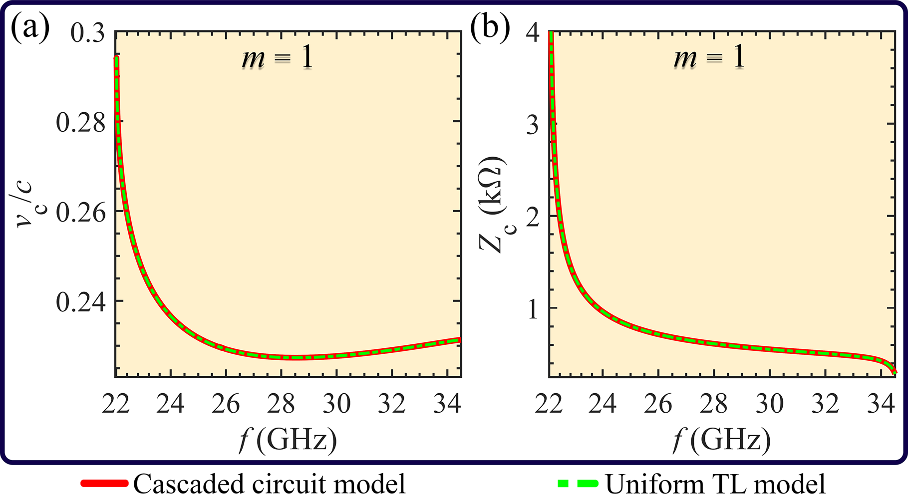
Figure 5: (a) Normalized phase velocity and (b) characteristic impedance of the first spatial harmonic ($m=1$) calculated by using the cascaded circuit model (solid red curve) described in Subsection III-B and the uniform TL model (dashed green curve) described in Subsection III-C.

TABLE I: Designed structural parameters for the serpentine waveguide SWS.

Description	Parameter	Length (mm)
The width of rectangular waveguide	$w$	$6.8$
The height of rectangular waveguide	$b$	$0.7$
The full period length	$d$	$4$
The whole straight waveguide length	$h$	$2.5$
The radius of beam tunnel	$r_{\mathrm{c}}$	$0.5$

Figure 4 shows the wavenumber, phase velocity and characteristic impedance of the EM modes in the cold serpentine waveguide obtained using theoretical and simulation methods. Figure 4(a) shows the wavenumber dispersion diagram of the modes in the serpentine waveguide, showing three spatial harmonics, obtained by varying the phase between periodic boundaries. The simulated results based on the CST Studio Suite eigenmode solver (dashed black curves) are in excellent agreement with the theoretical dispersion diagram calculated by the cascaded circuit model (solid red curves) discussed in Subsection III-B. The cutoff frequency of the designed serpentine waveguide is around $f_{\mathrm{c}}=22.15\>\mathrm{GHz}$. Then, the normalized phase velocity corresponding to the first spatial harmonic ($m=1$) as a function of frequency ranging from $22.15\>\mathrm{GHz}$ to $34.5\>\mathrm{GHz}$ is plotted in Fig. 4(b). There is excellent agreement between the results provided by the eigenmode solver (dashed black curve), cascaded circuit model (solid red curve) in Subsection III-B, and waveguide projection model (dashed blue curve) in Subsection III-D. As a general observation, the cascaded circuit model is more accurate than the waveguide projection model because mismatches due to circular bends and junctions are taken into account in this model. In addition, the characteristic impedance of the serpentine waveguide SWS is shown in Fig. 4(c).

In order to demonstrate that the serpentine waveguide can be modeled by a single straight uniform TL, we compare the results based on the uniform TL model with the cascaded circuit model. The calculated results for the first spatial harmonic in both cases are shown in Fig. 5(a) and (b), and we observe excellent agreement between these two theoretical methods. Also, previous studies, such as [17], utilized the uniform TL model that is very similar to what is discussed in this paper for the cold case. In contrast, in this paper we also develop a model for finding the “hot eigenmodes” dispersion of the device and the TWT gain. The accurate calculation of the characteristic parameters of the cold structure, i.e., $Z_{\mathrm{c}}$ and $v_{\mathrm{c}}$, has a vital role in our model. To reinforce this point, we note that one of the conclusions of [17] is that accurate determination of the small-signal gain in a serpentine waveguide TWT amplifier requires a precise evaluation of the phase velocity to within $0.5\%$ and the interaction impedance within $10\%$ of the actual parameters found by time-consuming full-wave eigenmode simulations. The calculated gain is very sensitive to these parameters, and requires correct phase velocity and interaction impedance specification. Sensitivity studies in [17] indicate that variations in the phase velocity of $0.5\%$ can result in $8\>\mathrm{dB}$ of variation in the predicted small-signal gain, while a $10\%$ variation in the interaction impedance can result in a $5\>\mathrm{dB}$ change in the predicted small-signal gain of the specific design.

V Interaction Impedance

In order to predict the performance of a TWT, one needs to determine the interaction (Pierce) impedance of the serpentine waveguide because amplifier gain is proportional to the cubic root of this parameter [29]. The interaction impedance is a measure of how much the on-axis electric field can velocity modulate electrons for a given EM power propagating along the length of the structure [45, Ch. 10]. In the ideal case, the e-beam is assumed to be very narrow. From Pierce theory, the interaction impedance for a thin beam is defined for a specific spatial harmonic $m$ as [45, Ch. 10]

$$Z_{\mathrm{P},m}\left(\beta_{\mathrm{c,}m}\right)=\frac{\left|E_{z,m}\left(\beta_{\mathrm{c,}m}\right)\right|^{2}}{2\beta_{\mathrm{c,}m}^{2}P},$$ (17)

where $\left|E_{z,m}\left(\beta_{\mathrm{c,}m}\right)\right|$ is the magnitude of the axial electric field phasor along the center of the cold SWS where the e-beam will be introduced, for a given phase constant and spatial harmonic $m$, and $P$ is the time-average power flux through the SWS at the given phase propagation constant $\beta_{\mathrm{c,}m}$ [45]. The quantity $\left|E_{z,m}\right|$ is the weight of the $m$th Floquet-Bloch spatial harmonics of the axial field decomposition $E_{z}\left(z,\beta_{\mathrm{c}}\right)=\sum_{m=-\infty}^{\infty}E_{z,m}\left(\beta_{\mathrm{c}}\right)e^{-j\beta_{\mathrm{c,}m}z}$. It is calculated by numerically obtaining the phasor of the axial electric field $E_{z}\left(z,\beta_{\mathrm{c}}\right)$ of the cold serpentine waveguide with beam tunnel using full-wave eigenmode simulations, followed by performing the Fourier transform in space

$$E_{z,m}\left(\beta_{\mathrm{c}}\right)=\frac{1}{d}\intop_{0}^{d}E_{z}\left(z,\beta_{\mathrm{c}}\right)e^{j\beta_{\mathrm{c,}m}z}dz.$$ (18)

In addition, the time average power flux is simply calculated as $P=W_{\mathrm{t}}v_{\mathrm{g}}/d$ [46], where $W_{\mathrm{t}}$ is the total EM energy of the wave stored in a unit cell, and the group velocity $v_{\mathrm{g}}=d\omega/d\beta_{\mathrm{c}}$ can be determined directly from the dispersion diagram by using numerical differentiation. The EM energy simulated within a single unit cell between periodic boundaries in the CST Studio Suite eigenmode solver is always $1~{}\mathrm{Joule}$. For a serpentine waveguide, the interaction impedance is typically evaluated within the first Brillouin zone (i.e., $m=1$), where the interaction occurs. Additionally, the e-beam diameter also influences the interaction impedance. For beam cross sections and beam tunnel diameters that are not infinitesimally thin, the longitudinal electric field and the interaction impedance within the beam tunnel can vary over the beam cross section area, becoming larger near the edges of the tunnel. As a consequence, the additional correction factor (average factor) should be considered in calculating the interaction impedance by taking into account the variation of the electric field within the interaction area (interaction gap) [47]. Additional analysis of the variation of the electric field distribution in the interaction area for the specific example can be found in Appendix C. Therefore, a modified or “effective interaction impedance” corresponding to each spatial harmonic considering the nonuniform electric field distribution in the interaction area is given by

$$Z_{\mathrm{P},\mathrm{e},m}=\left(1+\delta_{\mathrm{e}}\right)^{2}Z_{\mathrm{P},m},$$ (19)

where, $\delta_{\mathrm{e}}>0$ is the correction factor. The value of the correction factor can be found either by (i) averaging the EM axial field over the beam cross section, or (ii) by matching the maximum value of the theoretical and PIC-simulated gain at the synchronization frequency.

VI E-beam and EM Wave Interaction

The classical small-signal theory by J. R. Pierce is one of the most famous approaches used for TWT modeling and design [27, 28, 29, 30]. Our implementation based on the generalization of Pierce’s theory is summarized here following our previous work [31]. We follow the linearized equations that describe the space-charge wave as originally presented by Pierce.

The equivalent model for the TWT describes the EM wave traveling in a serpentine waveguide interacting with an e-beam flowing in the $z$ direction as shown schematically in Fig. 6. The electrons have an average velocity and linear charge density of $u_{0}$ and $\rho_{0}$, respectively. The e-beam has an average current $I_{0}=-\rho_{0}u_{0}$ in the $-z$ direction and an equivalent kinetic d.c. voltage as $V_{0}\approx u_{0}^{2}/\left(2\eta\right)$ for non-relativistic beams (assuming that thermal initial velocity of the electron is neglected) or $V_{0}=\left(\sqrt{1-\left(u_{0}/c\right)^{2}}-1\right)c^{2}/\eta$ for relativistic beams, where $c$ is the speed of light in a vacuum, $\eta=e/m=1.758820\times 10^{11}\>\mathrm{C/Kg}$ is the charge-to-mass ratio of the electron with charge $-e$ and rest mass $m$ [48, Ch. 3]. The small-signal modulations in the charge velocity $u_{\mathrm{b}}$ and charge density $\rho_{\mathrm{b}}$, describe the “space-charge wave”. The a.c. equivalent beam current and kinetic voltage are given by $i_{\mathrm{b}}=u_{\mathrm{b}}\rho_{0}+u_{0}\rho_{\mathrm{b}}$ and $v_{\mathrm{b}}=u_{\mathrm{b}}u_{0}/\eta$, where we have kept only the linear terms based on the small-signal approximation [30]. We implicitly assume a time dependence of $\exp\left(j\omega t\right)$, so the a.c. space-charge wave modulating the e-beam is described in the phasor domain with $V_{\mathrm{b}}\left(z\right)$ and $I_{\mathrm{b}}\left(z\right)$, as

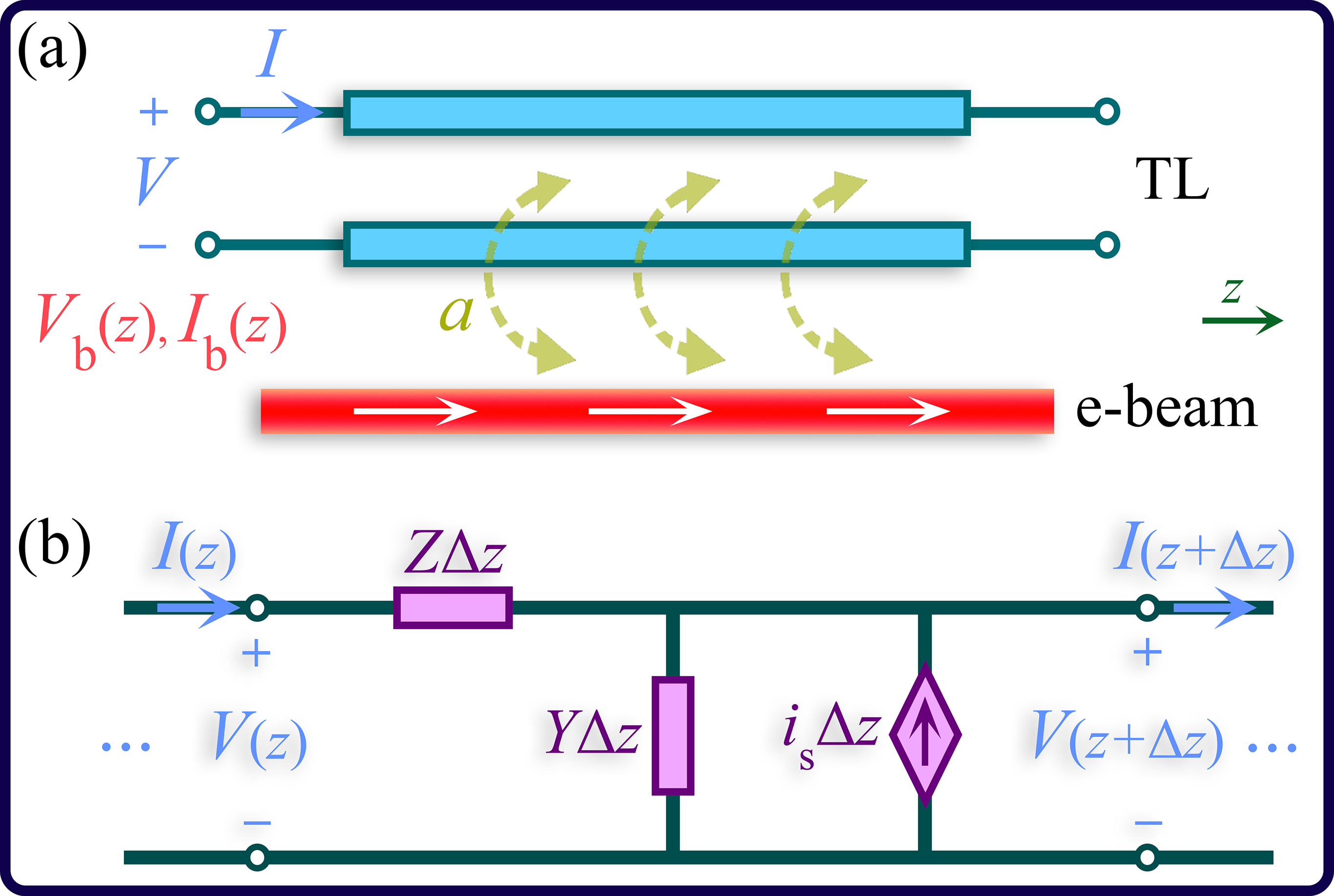
Figure 6: (a) Schematic of the equivalent TL coupled to the e-beam used to study the beam-EM wave interaction in the serpentine waveguide TWT. (b) Equivalent TL circuit showing the per-unit-length impedance, admittance and current generator $i_{\mathrm{s}}=-a\partial_{z}I_{\mathrm{b}}$ that represents the effect of the e-beam on the TL.

$$\frac{d}{dz}V_{\mathrm{b}}=-j\beta_{0}V_{\mathrm{b}}-aZI-j\frac{I_{\mathrm{b}}}{A\varepsilon_{0}\omega},$$ (20)

$$\frac{d}{dz}I_{\mathrm{b}}=-jgV_{\mathrm{b}}-j\beta_{0}I_{\mathrm{b}},$$ (21)

where $\beta_{0}=\omega/u_{0}$ is the space-charge wave equivalent phase constant (when neglecting plasma frequency effects), $g=I_{0}\beta_{0}/\left(2V_{0}\right)$, $Z$ is the equivalent TL distributed series impedance, and $I\left(z\right)$ is the equivalent TL current. The term $E_{\mathrm{w}}=aZI$ is the longitudinal electric field of the EM mode propagation in the SWS, affecting the bunching of the e-beam. In addition, the coefficient $a$ represents a coupling strength that describes how the e-beam couples to the TL, already introduced in [49, 31, 50] and [51, 52, Ch. 3] and investigated in more detail in Appendix D. Also, the term $E_{\mathrm{p}}=jI_{\mathrm{b}}/\left(A\varepsilon_{0}\omega\right)$ is the longitudinal electric field term arising from the nonuniform charge density that causes the so-called “debunching” [45, Ch. 10], where $A$ is the e-beam cross sectional area, and $\varepsilon_{0}$ is vacuum permittivity. This field is responsible of the repulsive forces in a dense beam of charged particles. Therefore, $E_{z}=E_{\mathrm{w}}+E_{\mathrm{p}}$ is the total longitudinal $z$-polarized electric field component in the hot structure (when also the e-beam is present) that modulates the velocity and bunching of the electrons. In serpentine waveguide TWTs, the beam-EM wave interaction occurs in the first spatial harmonic ($m=1$), so in this section we drop the subscript harmonic index $m$ for simplicity. The telegrapher’s equations,

$$\frac{d}{dz}V=-ZI,$$ (22)

$$\frac{d}{dz}I=-YV-a\frac{d}{dz}I_{\mathrm{b}},$$ (23)

describe the modal propagation in the SWS of the EM mode synchronizing with the e-beam in terms of equivalent TL voltage $V\left(z\right)$ and current $I\left(z\right)$ phasors, based on the equivalent TL model shown in Fig. 6(b). Figure 6(b) shows the distributed per-unit-length series impedance $Z$ and shunt admittance $Y$ as well as the term $i_{\mathrm{s}}=-a\left(dI_{\mathrm{b}}/dz\right)$ that represents an equivalent distributed current generator [53, 49, 31, 50]. This current generator accounts for the effect of the beam’s charge wave flowing in the SWS. It is well known that dependent sources are used to describe gain in transistors and linear amplifiers, which justifies this approach to model the e-beams effect on the TL. The frequency dependent parameters $Z$ and $Y$ could be obtained using the cascaded circuit model described in Subsection III-B as follows. We evaluate the phase velocity of the cold circuit EM modes $v_{\mathrm{c}}\left(\omega\right)=\omega/\beta_{\mathrm{c}}\left(\omega\right)$, where $\beta_{\mathrm{c}}\left(\omega\right)=\sqrt{-Z\left(\omega\right)Y\left(\omega\right)}$ is the phase propagation constant harmonic of the cold SWS mode interacting with the e-beam, and the equivalent TL characteristic impedance $Z_{\mathrm{c}}\left(\omega\right)$. Then, one could obtain the equivalent frequency-dependent distributed series impedance $Z\left(\omega\right)=j\beta_{\mathrm{c}}\left(\omega\right)Z_{\mathrm{c}}\left(\omega\right)$ and shunt admittance $Y\left(\omega\right)=j\beta_{\mathrm{c}}\left(\omega\right)/Z_{\mathrm{c}}\left(\omega\right)$.

For convenience, we define a state vector $\boldsymbol{\Psi}\left(z\right)=\left[V,I,V_{\mathrm{b}},I_{\mathrm{b}}\right]^{\mathrm{T}}$ ($\mathrm{T}$ indicates transpose operation) that describes the hot mode propagation, and rewrite (20), (21), (22), and (23) in matrix form as

$$\frac{d}{dz}\boldsymbol{\Psi}(z)=-j\mathbf{\underline{M}}\boldsymbol{\Psi}(z),$$ (24)

$$\underline{\mathbf{M}}=\left[\begin{array}[]{rrrr}0&\beta_{\mathrm{c}}Z_{\mathrm{c}}&0&0\\ \beta_{\mathrm{c}}/Z_{\mathrm{c}}&0&-ag&-a\beta_{0}\\ 0&a\beta_{\mathrm{c}}Z_{\mathrm{c}}&\beta_{0}&\zeta_{\mathrm{sc}}\\ 0&0&g&\beta_{0}\end{array}\right],$$ (25)

where $\underline{\mathbf{M}}$ is the $4\times 4$ system matrix. Here, we have used directly the primary TL parameters $\beta_{\mathrm{c}}\left(\omega\right)$ and $Z_{\mathrm{c}}\left(\omega\right)$ instead of $Z\left(\omega\right)$ and $Y\left(\omega\right)$. In the above system matrix, $\zeta_{\mathrm{sc}}$ is the space-charge parameter related to the debunching of beam’s charges, and is given by [31]

$$\zeta_{\mathrm{sc}}=\frac{R_{\mathrm{sc}}}{A\varepsilon_{0}\omega}=\frac{2V_{0}\omega{}_{\mathrm{q}}^{2}}{\omega I_{0}u_{0}},$$ (26)

where $\omega_{\mathrm{q}}=R_{\mathrm{sc}}\omega_{\mathrm{p}}$ is the reduced plasma angular frequency, $\omega_{\mathrm{p}}=\sqrt{-\rho_{0}\eta/\left(A\varepsilon_{0}\right)}=\sqrt{I_{0}u_{0}/\left(2V_{0}A\varepsilon_{0}\right)}$ is the plasma frequency [54], and $R_{\mathrm{sc}}$ is the plasma frequency reduction factor [55, 56]. The term $R_{\mathrm{sc}}$ accounts for reductions in the magnitude of the axial component of the space-charge electric field due to either a finite beam radius or proximity to the surrounding conducting walls of the e-beam tunnel [57] (details in Appendix E). As shown in Appendix D, the coupling strength coefficient $a$ is found by using the formula

$$a=\sqrt{\frac{Z_{\mathrm{P,e}}}{Z_{\mathrm{c}}}},$$ (27)

and it is frequency dependent as shown later on. In summary, all the parameters of the presented model are found using cold simulations of the EM mode in the serpentine waveguide SWS to estimate the performance of the hot structure.

VI-A Characteristic Equation and Electronic Beam Admittance

Assuming a state vector $z$-dependence of the form $\boldsymbol{\Psi}\left(z\right)\propto\exp\left(-jkz\right)$, where $k$ is the complex-valued wavenumber of a hot mode in the interactive system, leads to the eigenvalue problem $k\boldsymbol{\Psi}\left(z\right)=\mathbf{\underline{M}}\boldsymbol{\Psi}\left(z\right)$. The resulting modal dispersion characteristic equation is given by

$$\begin{array}[]{c}D\left(\omega,k\right)=\det\left(\mathbf{\underline{M}}-k\mathbf{\underline{I}}\right)=k^{4}-k^{3}\left(2\beta_{0}\right)\\ \\ +k^{2}\left(\beta_{0}^{2}-\beta_{\mathrm{q}}^{2}-\beta_{\mathrm{c}}^{2}+a^{2}g\beta_{\mathrm{c}}Z_{\mathrm{c}}\right)+k\left(2\beta_{\mathrm{c}}^{2}\beta_{0}\right)\\ \\ -\beta_{\mathrm{c}}^{2}\left(\beta_{0}^{2}-\beta_{\mathrm{q}}^{2}\right)=0,\end{array}$$ (28)

where $\beta_{\mathrm{q}}=\omega_{\mathrm{q}}/u_{0}=\sqrt{\zeta_{\mathrm{sc}}g}$ is the phase constant of space-charge wave. The solution of (28) leads to four modal complex-valued wavenumbers of the four hot modes in the interactive system. The characteristic equation is rewritten as follows

$$\left(k^{2}-\beta_{\mathrm{c}}^{2}\right)\left[\left(k-\beta_{0}\right)^{2}-\beta_{\mathrm{q}}^{2}\right]=-a^{2}gk^{2}\beta_{\mathrm{c}}Z_{\mathrm{c}},$$ (29)

to stress that the term $-a^{2}g\beta_{\mathrm{c}}Z_{\mathrm{c}}k^{2}$ ($=-g\beta_{\mathrm{c}}Z_{\mathrm{P,e}}k^{2}$) indicates the coupling between the two dispersion equations of the isolated EM waves in the cold SWS $\left(k^{2}-\beta_{\mathrm{c}}^{2}\right)=0$, and isolated charge waves $\left[\left(k-\beta_{0}\right)^{2}-\beta_{\mathrm{q}}^{2}\right]=0$. Here, only parameters obtained from cold SWS simulations are used to find the dispersion of the four hot modes. For a given eigenmode, the e-beam interaction with the EM wave could be completely modeled as an active TL with a voltage-dependent current source, as shown schematically in Fig. 6, given by [49]

$$i_{\mathrm{s}}=jakI_{\mathrm{b}}=-Y_{\mathrm{b}}V,$$ (30)

where the electronic beam admittance per unit length $Y_{\mathrm{b}}$ is

$$Y_{\mathrm{b}}=-j\frac{a^{2}gk^{2}}{\left[\left(k-\beta_{0}\right)^{2}-\beta_{\mathrm{q}}^{2}\right]}.$$ (31)

This admittance is a generalization of the one already provided in [49] since here we have included the space charge effect $\beta_{\mathrm{q}}^{2}=g\zeta_{\mathrm{sc}}$.

VI-B TWT Amplifier Gain

We describe the theoretical calculation to compute the gain of a TWT amplifier using the circuit model illustrated in Fig. 7, where a matched resistance is considered for the source generator $R_{\mathrm{S}}$, and the output is terminated by the matched load $R_{\mathrm{L}}$. The serpentine waveguide TWT is modeled by the system matrix $\underline{\mathbf{M}}$ described earlier, input state vector of $\boldsymbol{\Psi}_{1}=\left[V^{\mathrm{i}},I^{\mathrm{i}},V_{\mathrm{b}}^{\mathrm{i}},I_{\mathrm{b}}^{\mathrm{i}}\right]^{\mathrm{T}}$ calculated at $z=0$, and output state vector of $\boldsymbol{\Psi}_{2}=\left[V^{\mathrm{o}},I^{\mathrm{o}},V_{\mathrm{b}}^{\mathrm{o}},I_{\mathrm{b}}^{\mathrm{o}}\right]^{\mathrm{T}}$ calculated at $z=Nd$, i.e., at the end of the TWT, where $N$ indicates the number of unit cells. The output state vector is calculated as $\boldsymbol{\Psi}_{2}=\underline{\mathbf{T}}\boldsymbol{\Psi}_{1}$, where $\underline{\mathbf{T}}=\exp\left(-j\underline{\mathbf{M}}Nd\right)$ is the TWT transfer matrix.

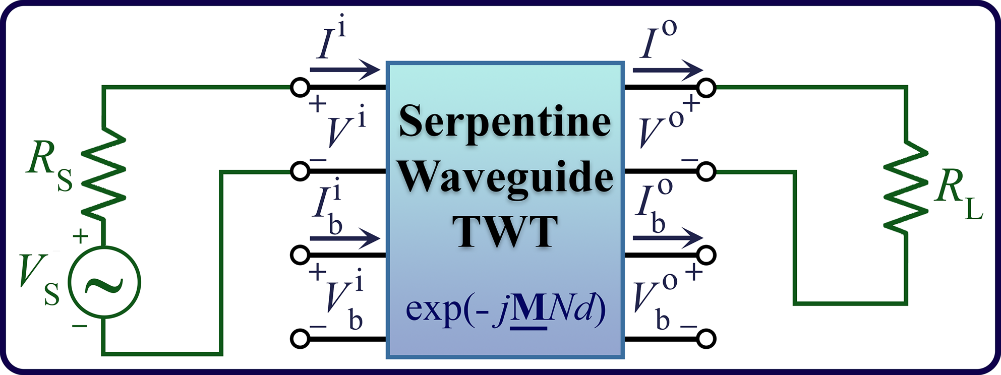
Figure 7: Circuit model for gain calculation considering frequency-dependent resistances for the source and load ($R_{\mathrm{S}}$ and $R_{\mathrm{L}}$).

In the model, we use the following boundary conditions at $z=0$ and $z=Nd$,

$$\left\{\begin{array}[]{l}V_{\mathrm{b}}^{\mathrm{i}}=0,\;I_{\mathrm{b}}^{\mathrm{i}}=0\\ V^{\mathrm{i}}+I^{\mathrm{i}}R_{\mathrm{S}}=V_{\mathrm{S}},\;V^{\mathrm{o}}-I^{\mathrm{o}}R_{\mathrm{L}}=0\end{array}\right.$$ (32)

In these equations, the source resistance $R_{\mathrm{S}}$ and load resistance $R_{\mathrm{L}}$ are assumed to be equal to the frequency-dependent characteristic impedance of the serpentine waveguide $Z_{\mathrm{c}}$, and $V_{\mathrm{S}}$ is the generator voltage source. We solve the system of equations at each frequency and calculate the equivalent circuit current and voltage (proportional to the electric and magnetic fields) at the TWT output port. Then, we calculate the output power $P_{\mathrm{out}}=\left|V^{\mathrm{o}}\right|^{2}/\left(2R_{\mathrm{L}}\right)$, and the available input power $P_{\mathrm{av}}=\left|V_{\mathrm{S}}\right|^{2}/\left(8R_{\mathrm{S}}\right)$ (also denoted as incident power) to obtain the frequency-dependent gain as $G=P_{\mathrm{out}}/P_{\mathrm{av}}$. An explanation of the calculation method is provided in Appendix F.

VII Validation of Model for Hot Structure

In order to investigate the accuracy of the presented model for the interaction, we compare the theoretically calculated gain versus frequency results from our model with those numerically obtained from the commercial PIC software CST Particle Studio. As explained in Section V, in our model we consider the effective interaction impedance, which describes the strength of beam-EM mode interaction in the TWT. In this paper, the correction factor $\delta_{\mathrm{e}}$ is calculated by matching the maximum gain value from the theoretical model with the one obtained by only one PIC simulation that occurs at the synchronization frequency, $Z_{\mathrm{P}}$ is determined from (17) by post-processing the data extracted from CST eigenmode simulations and $v_{\mathrm{c}}$ is calculated by theoretical circuit models, i.e., a cascaded circuit model.

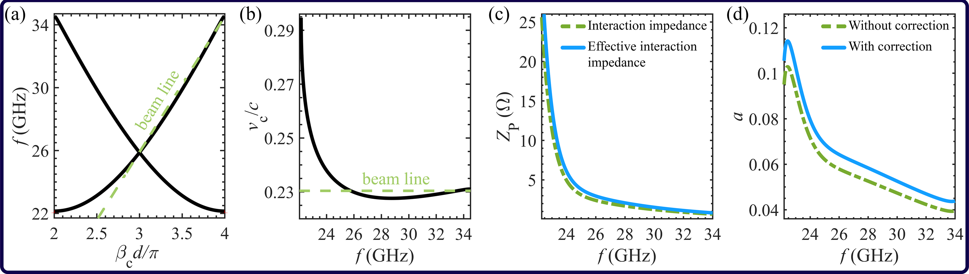
Figure 8: Cold results: (a) Dispersion curve and (b) normalized phase velocity of the modes in the cold serpentine waveguide SWS in the first spatial harmonic. (c) The on-axis interaction impedance of the serpentine waveguide SWS at the center of the beam tunnel with (solid blue) and without (dashed green) considering the correction factor $\delta_{\mathrm{e}}$. (d) The frequency-dependent value of the coupling strength coefficient $a$ with (solid blue) and without (dashed green) correction factor.

In this study, synchronization with the first spatial harmonic of the SWS is selected for low beam voltage operation. However, for simplicity of notation, we drop the harmonic index number and we will call the circuit modal wavenumber and phase velocity belonging to the $m=1$ spatial harmonic simply as $\beta_{\mathrm{c}}$ and $v_{\mathrm{c}}$. We consider a serpentine waveguide SWS with the geometry parameters listed in Table I. The e-beam has $I_{0}=10\>\mathrm{mA}$ and a radius $r_{\mathrm{b}}=0.35\>\mathrm{mm}$ and we end up with a tunnel filling factor of $\left(r_{\mathrm{b}}/r_{\mathrm{c}}\right)^{2}=0.5$. For the e-beam, the normalized phase velocity $u_{0}/c$ is set to be $0.230$. This value corresponds to an average kinetic voltage of $V_{0}=14.077\>\mathrm{kV}$ for the e-beam. Additionally, a uniform longitudinal magnetic field of $0.8\;\mathrm{T}$ was applied to confine the e-beam. The cold dispersion diagram and beam line are illustrated in Fig. 8(a) where the beam line with normalized phase velocity of $u_{0}/c=0.230$ is superimposed to the wavenumber of the EM mode, in the SWS on both left and right of the $3\pi$ point. Additionally, the beam line may synchronize with the EM backward mode near $3\pi$ at the intersection frequency which may result in parasitic oscillations [41]. So, in the design of a long serpentine waveguide TWT, attenuators can be used to mitigate oscillation risk. However, this issue is not discussed here, and how the presented model can be adapted to cases with attenuators will be studied in our future work. The frequency-dependent interaction impedance calculated at the beam center for the first spatial harmonic by using (17) is shown in Fig. 8(c). In this example, the interaction impedance correction factor is considered to be $\delta_{\mathrm{e}}=0.11$, which is a relatively small factor. We show both the calculated interaction impedance without correction factor $Z_{\mathrm{P}}$ (see (17)) and effective interaction impedance with correction factor $Z_{\mathrm{P,e}}$ (see (19)) in Fig. 8(c) by using dashed green and solid blue curves respectively. The on-axis interaction impedance approaches very high values near the waveguide cutoff frequency at $f_{\mathrm{c}}=22.15\>\mathrm{GHz}$ and gradually drops as the frequency grows further away from the cutoff frequency. The frequency-dependent value of the coupling strength coefficient without considering correction factor, $a=\sqrt{Z_{\mathrm{P}}/Z_{\mathrm{c}}}$, and with correction factor, $a=\sqrt{Z_{\mathrm{P,e}}/Z_{\mathrm{c}}}=(1+\delta_{\mathrm{e}})\sqrt{Z_{\mathrm{P}}/Z_{\mathrm{c}}}$, are shown in Fig. 8(d).

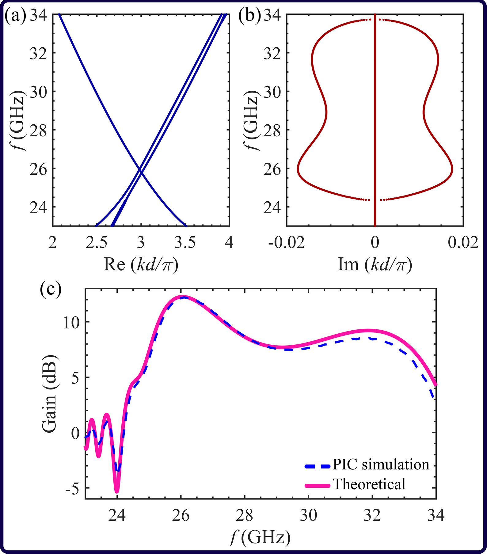
Figure 9: Hot results: The (a) real and (b) imaginary parts of complex-valued wavenumbers of hot modes by varying frequency. (c) TWT gain versus frequency predicted by the proposed theoretical model (solid pink), compared to 3D PIC simulations (dashed green).

According to the intersection of the cold EM mode phase velocity curve $v_{\mathrm{c}}$ and the beam line in Fig. 8(b), we observe beam-EM wave full synchronization at $25.73\>\mathrm{GHz}$ and $33.52\>\mathrm{GHz}$, where high amplification is expected to occur. The real and imaginary parts of the complex-valued wavenumber of the hot modes (i.e., accounting for the beam-EM wave interaction) are calculated by (29) and shown in Figs. 9(a) and (b). The amplification regime is obtained when there is a hot mode with $\mathrm{Im}\left(k\right)>0$. The numerical gain versus frequency diagram is theoretically calculated by the method described in Subsection VI-B for the serpentine waveguide TWT with $N=40$ unit cells ($160\>\mathrm{mm}$ in length) and input power of $P_{\mathrm{in}}=0\>\mathrm{dBm}$. It is compared with the one obtained by numerically intensive 3D PIC simulations, resulting in excellent agreement. The comparison also validated the value of the interaction impedance correction factor $\delta_{\mathrm{e}}=0.11$. Since the analysis is in the linear regime, instead of using $N=40$ unit cells, a quick simulation to estimate the correction factor $\delta_{\mathrm{e}}$ was done based on only $N=10$ unit cells. However, as a check we also verified that we obtained the same value when considering $N=40$.

The theoretical and PIC simulated gain versus frequency are illustrated in Fig. 9(c) by solid pink and dashed blue curves, respectively. The agreement is excellent, indicating the accuracy of the model. Additionally, as predicted, maximum gains are obtained around synchronization frequencies. The total number of mesh cells in the simulation is approximately 2.6 million and a steady state output signal is seen after a transient time of $10\>\mathrm{ns}$ elapses. We use a sinusoidal signal as an excitation signal in the PIC simulation and a frequency sweep is performed to calculate output power in the selected frequency band. As shown in Fig. 9(c), the 3-dB bandwidth is $9.37\%$ covering from $25.21\>\mathrm{GHz}$ to $27.65\>\mathrm{GHz}$. Also, the maximum amplifier gain of $12.27\>\mathrm{dB}$ is obtained at $26.04\>\mathrm{GHz}$. We also investigated another example with a wider e-beam with tunnel filling factor of $\left(r_{\mathrm{b}}/r_{\mathrm{c}}\right)^{2}=0.95$. In this case, the correction factor is $\delta_{\mathrm{e}}=0.18$. This value is explainable since according to Fig. 14(c) and (d) we observe bigger values of electric fields near the beam tunnel wall which leads to stronger beam-EM wave interaction. Note that the purpose of this paper is not to design a TWT that can compete with conventional designs, but to showcase a simple and accurate model to predict TWT performance.

VIII Parameter Study

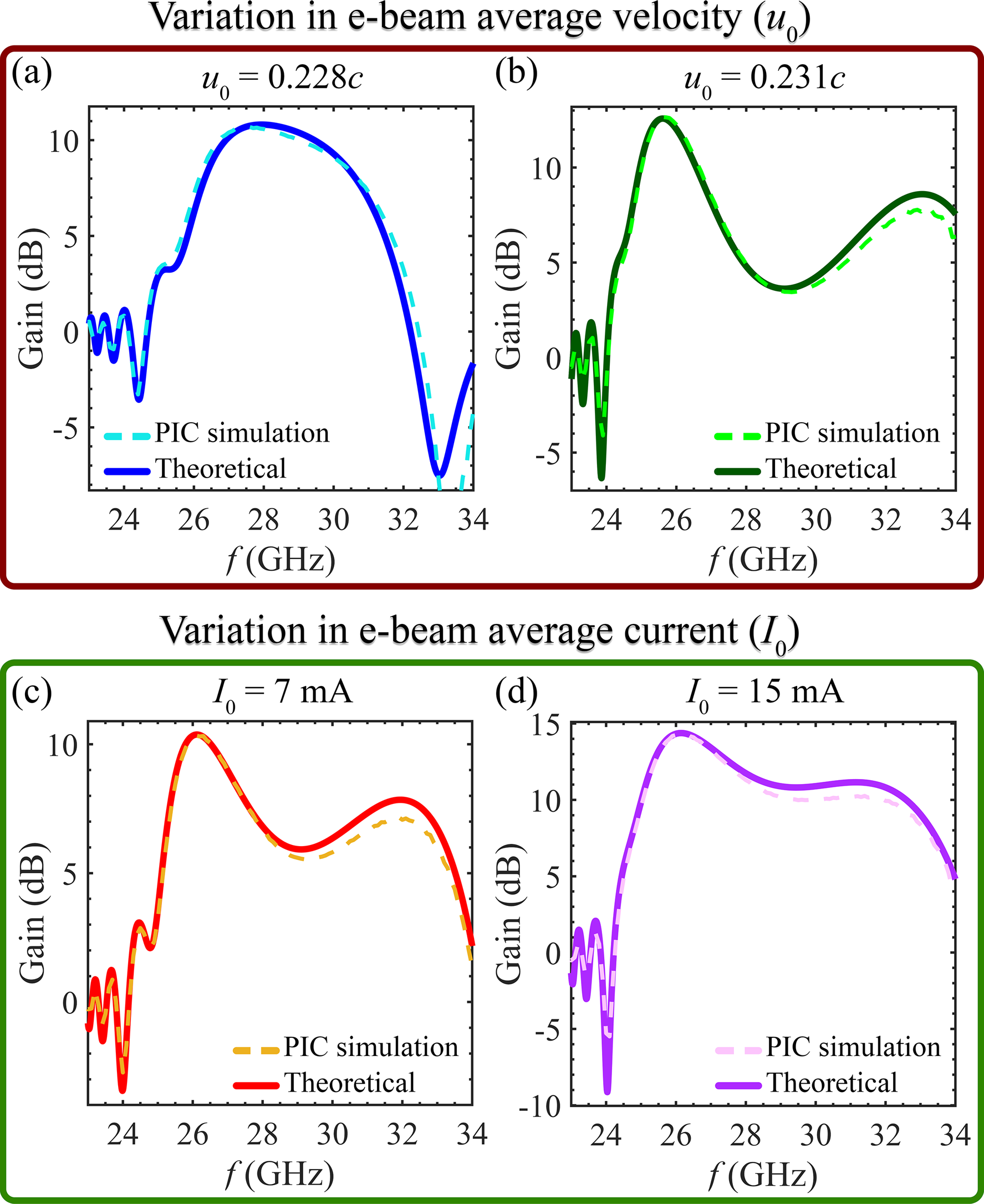
Figure 10: Comparison of gain versus frequency for a serpentine waveguide TWT calculated using our theoretical model and PIC simulations. In the first row, we show gain diagram by varying e-beam average phase velocity as (a) $u_{0}=0.228c$ and (b) $u_{0}=0.231c$. In the second row, we illustrate gain diagram by varying e-beam average current as (c) $I_{0}=7\>\mathrm{mA}$ and (d) $I_{0}=15\>\mathrm{mA}$. The solid curves in these plots show the results obtained via PIC simulation whereas dashed curves are obtained based on the proposed theoretical model.

To validate the presented model, a variety of simulation runs and comparisons have been carried out. We will apply the same correction factor $\delta_{\mathrm{e}}=0.11$ obtained in the previous section to all the following examples. In fact, the effective interaction impedance and correction factor $\delta_{\mathrm{e}}$ are identical for all examples, even when changing the e-beam parameters, number of unit cells and input power in the linear regime. First, we vary $u_{0}$ to change the synchronization frequency but leave all other parameters unchanged, which are equal to the parameters used in Section VII. In Fig. 10(a), we select $u_{0}=0.228c$, which is $0.002c$ slower than the value used in the previous example. In this case, the forward branch of the modal dispersion diagram is approximately linear in the vicinity of the optimum frequency (i.e., the phase velocity remains almost constant). Here, the 3-dB bandwidth is $15.87\%$ of the center frequency covering from $26.27\>\mathrm{GHz}$ to $30.70\>\mathrm{GHz}$ and the maximum amplifier gain of $10.82\>\mathrm{dB}$ is predicted at $27.93\>\mathrm{GHz}$. Consequently, by establishing optimum synchronization, we can dramatically increase bandwidth. Next, in Fig. 10(b) we increase the e-beam phase velocity to $u_{0}=0.231c$, which leads to synchronization around $f_{\mathrm{sync}}=25.5\>\mathrm{GHz}$ and $f_{\mathrm{sync}}=34.26\>\mathrm{GHz}$, and calculate the gain. In these two plots, we also illustrate the theoretically calculated gain based on the proposed theoretical method, and we observe excellent agreement between theoretical (solid curves) and PIC simulation (dashed curves) results. We stress that we did not have to recalculate the correction factor $\delta_{\mathrm{e}}$ that was already calculated in the example in the previous section.

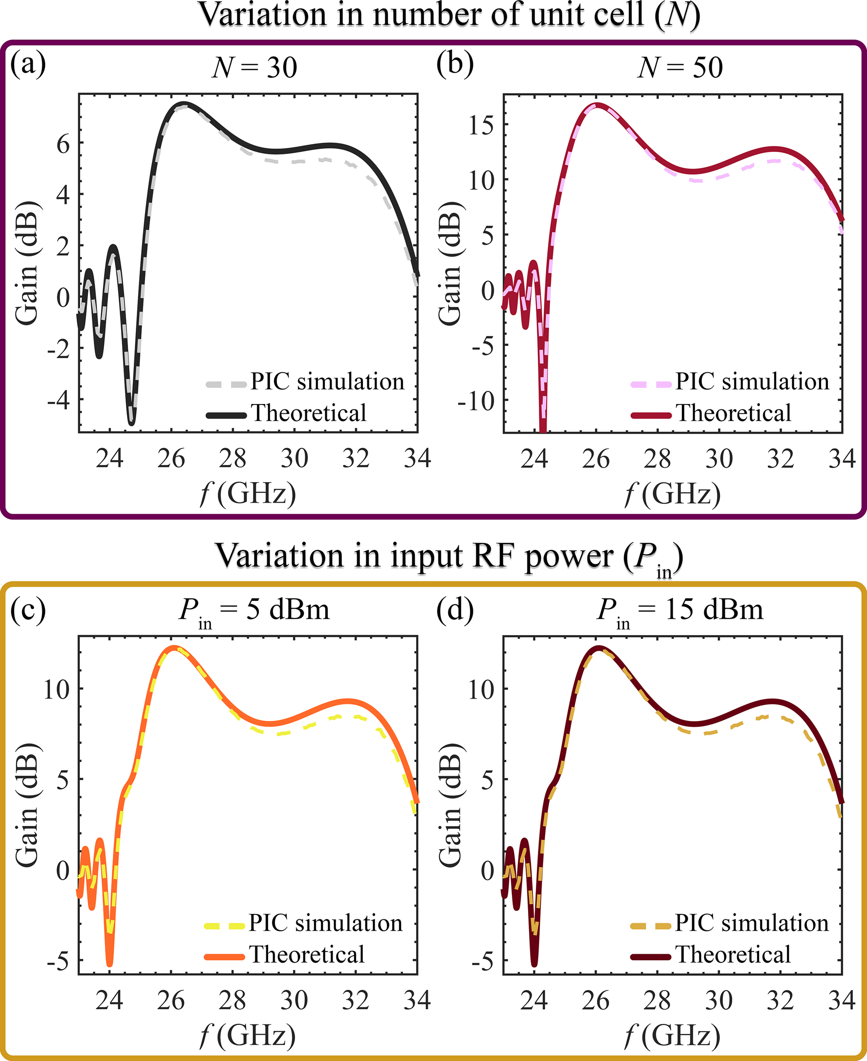
Figure 11: Comparison of gain versus frequency for a serpentine waveguide TWT calculated using our theoretical model and PIC simulations. In the first row, we show gain diagram by varying number of unit cells as (a) $N=30$ and (b) $N=50$. In the second row, we illustrate gain diagram by varying input power as (c) $P_{\mathrm{in}}=5\>\mathrm{dBm}$ and (d) $P_{\mathrm{in}}=15\>\mathrm{dBm}$. The solid curves in these plots show the results obtained via PIC simulation whereas dashed curves are obtained based on the proposed theoretical model.

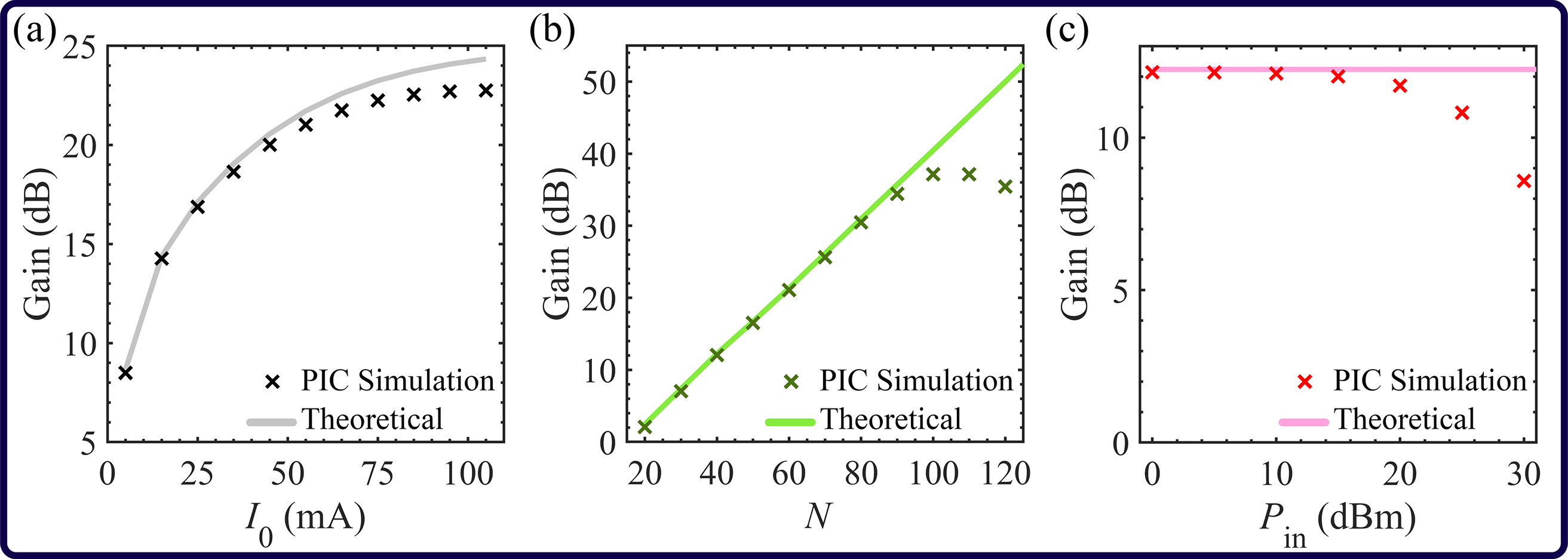
Figure 12: Comparison of gain versus frequency for a serpentine waveguide TWT calculated using our developed theoretical model (solid curves) and PIC simulations (dashed curves). In these plots, we change (a) e-beam average current, (b) number of unit cells, and (c) input power to show the accuracy of our theoretical calculation in the linear regime.

In the next step, the gain diagrams are calculated for the e-beam average currents of $I_{0}=7\>\mathrm{mA}$ and $I_{0}=15\>\mathrm{mA}$, shown in Figs. 10(c) and (d). All the other parameters are as described in the previous section. The maximum gain in both cases occurs approximately at the same frequency since the e-beam phase velocity is equal in both examples. On the other hand, the maximum gain for the current value of $I_{0}=15\>\mathrm{mA}$ is much bigger than the gain value for $I_{0}=7\>\mathrm{mA}$. Hence, it is critical to choose the right value for the e-beam current to avoid saturation. The solid curves obtained based on the proposed theoretical model show good agreement with the dashed curves calculated using PIC simulation. It is important to note that the correction factor $\delta_{\mathrm{e}}=0.11$ that was calculated in the previous section did not need to be adjusted or recalculated.

Our next step is to demonstrate how selecting the number of unit cells affects the gain and how this gain can be calculated accurately by the proposed model, still retaining the same correction factor $\delta_{\mathrm{e}}=0.11$ that was already calculated in the example in the previous section. The gain diagrams by varying the number of unit cells as $N=30$ and $N=50$ are calculated and shown in Figs. 11(a) and (b). In both cases, the e-beam has the same phase velocity, so maximum gain occurs roughly at the same frequency. The solid curves calculated by the theoretical model show excellent agreement with the dashed curves obtained by numerically intensive PIC simulations. Increasing the number of interaction unit cells too much will eventually result in undesirable oscillations when the small-signal gain becomes too high (e.g. above the practical limit of 30 dB for a single-stage TWT). Therefore, it is critical to consider the proper number of unit cells to prevent oscillations. As a result of using the longer device for higher gain extraction, we should use sever in the design which will be investigated in detail in our future work.

Next, we show the effect of input power variation on the gain diagram, but still retaining the same correction factor $\delta_{\mathrm{e}}=0.11$ that was already calculated in the example in the previous section. Since our method is based on small-signal approximation, we neglected the effect of nonlinear terms in our model. We provide two different examples with $P_{\mathrm{in}}=5\>\mathrm{dBm}$ and $P_{\mathrm{in}}=15\>\mathrm{dBm}$ and the calculated results are presented in Figs. 11(c) and (d). In comparison to the dashed curves obtained by PIC simulations, the theoretical results represented by solid curves exhibit good agreement.

As a last analysis, we calculate the gain at the synchronization frequency of $f_{\mathrm{sync}}=26\>\mathrm{GHz}$ by assuming the parameters used in Section VII. The gain diagram by varying the e-beam average current is shown in Fig. 12(a). In this plot, the theoretical gain is shown by a solid curve and the cross sign shows the corresponding simulation gain obtained from PIC simulation at sampled currents. When the e-beam current is increased, saturation occurs, so designers should choose the proper current value carefully. The analogous analysis is provided by varying the number of unit cells and the calculated gain at the synchronization frequency by both theoretical and PIC simulation is shown in Fig. 12(b). The simulation results confirm the calculated gain value when the number of unit cells is lower than 90 elements. It is significant to note that we did not use sever in the design of TWTs and all the simulations are provided for single-stage TWT. Finally, Fig. 12(c) shows the linear and saturation regions of the TWT depending on different input powers. The analysis shows that by increasing power we move into a nonlinear regime and the calculated results based on linear approximation will not be reliable. Again, it should be noted that the correction factor value in these plots has not changed from previous examples.

IX Conclusion

We have presented an extended analytical model for studying beam-EM wave interaction in a serpentine waveguide TWT that considers space-charge effects and dispersive waveguide parameters to predict gain in TWT amplifiers. The method is simple because it uses an equivalent circuit model to calculate the SWS cold (i) modal wavenumber, (ii) characteristic impedance, and (iii) the interaction impedance, which are all frequency dependent. We added a frequency-independent correction factor $\delta_{\mathrm{e}}$ to the interaction impedance, to model the nonuniform beam-EM wave interaction in the overlapping region of the e-beam and SWS longitudinal electric field. A theoretical method is used to predict the gain versus frequency and complex-valued wavenumber of the hot modes, and the results are compared with numerically intensive PIC simulations. The proposed method has been found always in good agreement with PIC simulations and much faster and flexible. For example, the flexibility of our method has been shown by changing the e-beam parameters, number of unit cells, and input power and by comparing the theoretical gain results with numerical gain results based on PIC simulations. The results consistently showed that our model is accurate and efficient at predicting serpentine waveguide TWT amplification characteristics.

Appendix A Definition of Voltage and Current

We use the equivalent representation in [34, 58] that models the rectangular waveguide as a TL with equivalent voltage and current. Following the derivation in [34, 58] for the TE10 mode in a straight rectangular waveguide and using the coordinates shown in the inset of Fig. 3, the transverse fields can be written. Then, the discrete voltages and the currents that represent the EM state in the phasor domain at different rectangular cross sections of the waveguide are defined as

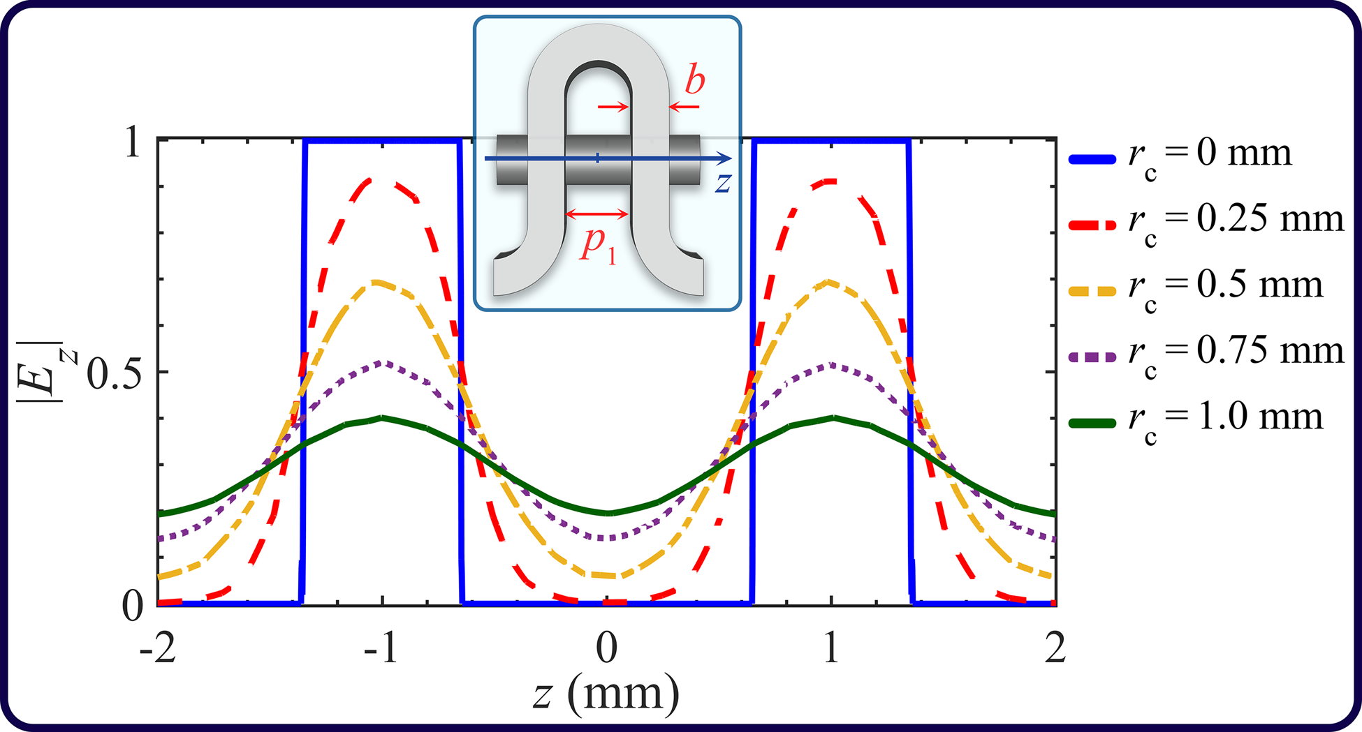
Figure 13: The on-axis $z$-component of electric field distribution as a function of longitudinal position $z$ in a one unit cell with $d=4\>\mathrm{mm}$, at the center of beam tunnel (i.e., $r=0$) for five beam tunnel radii $r_{\mathrm{c}}$. The calculated values are normalized to the maximum value of the $z$-component of the electric field in the interaction area when $r_{\mathrm{c}}=0$, i.e., the case without tunnel.

$$V_{n}=\sqrt{\frac{wb}{2}}E_{y,n},\;I_{n}=-\sqrt{\frac{wb}{2}}H_{x,n},$$ (33)

where $E_{y,n}$ and $H_{x,n}$ are the transverse electric and magnetic fields of the TE10 mode calculated at the center of the rectangular waveguide cross section as shown in Fig. 3, respectively. The proper normalization of voltages and currents in (33) provides the power carried by the TE10 mode

$$P_{n}=\frac{1}{2}\iint_{S}\mathrm{Re}\left(-E_{y,n}H_{x,n}^{*}\right)dxdy=\frac{1}{2}\mathrm{Re}\left(V_{n}I_{n}^{*}\right),$$ (34)

where $S=wb$ shows cross section area. Then, we define wave impedance that relates the transverse electric and magnetic fields as $Z_{\mathrm{TE}}=V_{n}/I_{n}=-E_{y,n}/H_{x,n}$.

Appendix B Longitudinal Fields in The Beam Tunnel

A number of works analyzed the effect of variation in the tunnel gap between the walls of the waveguide and the effect of thin interaction gap ($b$ in Fig. 13) [9, 59, 60, 61, 12, 13]. In addition, the tunnel between the straight waveguide sections ($p_{1}=d/2-b$ in Fig. 13) should be long enough to prevent the guided EM wave from directly coupling between straight sections via the beam tunnel, which operates below the cutoff [15, 16]. The analysis of the electric field distribution in the beam tunnel and interaction area of the cold single unit cell is shown in Fig. 13. The parameters used in this example are the same as those listed in Table I and we illustrate the on-axis $z$-component of electric field at the center of beam tunnel by varying beam tunnel radius $r_{\mathrm{c}}$.

Figure 14: The on-axis $z$-component of electric field distribution in the beam tunnel area in a cold serpentine waveguide SWS: (a) Over the longitudinal cross section, i.e., at $x=0$ plane; (b) in the interaction area at three different transverse cross section planes with $z_{0}=0.7\>\mathrm{mm}$, $z_{0}=0.85\>\mathrm{mm}$ and $z_{0}=1\>\mathrm{mm}$; (c) in the $x$ direction, with $y=0$, at three different $z_{0}$ coordinate; (d) at three different radii $r_{0}$, along the beam tunnel.

Appendix C Longitudinal Fields in The Interaction Regions

The magnitude of the $z$-component of electric field distribution at the center of the longitudinal cross section (the $x=0$ plane) of a cold serpentine waveguide is shown in Fig. 14(a). For better illustration, the $z$-component magnitude in the beam and EM wave interaction area at various transverse cross sections of $z_{0}=0.7\>\mathrm{mm}$, $z_{0}=0.85\>\mathrm{mm}$ and $z_{0}=1\>\mathrm{mm}$ is shown in Fig.14(b). We can see that the electric field magnitude increases near the beam tunnel perimeter. Also, the magnitude of the $z$-component of the electric field in a straight line in the $x$ direction, with $y=0$, at three different $z$ values is depicted in Fig. 14(c). The magnitude of the $z$-component of the electric field is also calculated at different radii inside the beam tunnel as shown in Fig. 14(d). These plots demonstrate that the minimum field value is obtained at the center of the beam tunnel and that the magnitude of $E_{z}$ increases gradually with an increasing radius. Thus, in the interaction area, the minimum interaction impedance is calculated at the center of the beam tunnel, i.e., at $r=0$. To account for the nonuniform distribution of the longitudinal electric field in the interaction area, the interaction impedance should be multiplied by a correction factor, i.e., $\left(1+\delta_{\mathrm{e}}\right)^{2}$. Since the electric field magnitude is greater near the tunnel wall, the correction factor should be greater than one ($\delta_{\mathrm{e}}\geq 0$).

Appendix D Coupling Strength Coefficient

The characteristic impedance of a mode guided by a cold waveguide is $Z_{\mathrm{c}}$ and by using this value, matching networks can be designed to terminate the input and output ends of the TWT. In contrast, in the Pierce model, the characteristic impedance of the equivalent TL that represents EM synchronization is the interaction impedance $Z_{\mathrm{P}}$. These two dispersive impedances are related by a frequency-dependent coupling strength coefficient discussed here. Other works have used this coupling strength coefficient introduced as an ad-hoc parameter, including [51, 49, 62, 63, 64, 52, 31, 65, 33, 66, 26]. Considering the modal propagation in the equivalent TL, the $z$-component of the a.c. electric field induced on the cold SWS was related to the phenomenological coupling strength coefficient $a$ as [49, 31]

$$E_{z}=-a\frac{dV\left(z\right)}{dz}.$$ (35)

The equivalent voltage on the TL is related to the per-unit length impedance and equivalent current as $dV\left(z\right)/dz=-ZI\left(z\right)$. For a lossless TL, the per-unit-length impedance is calculated by $Z=j\beta_{\mathrm{c}}Z_{\mathrm{c}}$. Then, we relate the equivalent voltage and current of the TL via the characteristic impedance by

$$\frac{dV\left(z\right)}{dz}=-j\beta_{\mathrm{c}}Z_{\mathrm{c}}I\left(z\right).$$ (36)

Substituting (36) in (35), we obtain the relation between the axial electric field of the guided mode and the equivalent current of TL by

$$E_{z}=ja\beta_{\mathrm{c}}Z_{\mathrm{c}}I\left(z\right).$$ (37)

Then, the interaction impedance $Z_{\mathrm{P}}$ is calculated by (17) for the interacting harmonic (i.e., $m=1$). Here, we derive the coupling strength coefficient in terms of $Z_{\mathrm{c}}$ and $Z_{\mathrm{P}}$. By substituting $E_{z}$ from (37) and time-average power along the TL $P=Z_{\mathrm{c}}\left|I\left(z\right)\right|^{2}/2$ in (17), the interaction impedance and characteristic impedance of the SWS are related through the coupling strength coefficient $a$, as $a=\sqrt{Z_{\mathrm{P}}/Z_{\mathrm{c}}}$. Using this relation between the characteristic impedance and the interaction impedance, one can transform the TL equivalent voltage and current of the state vector and system matrix in (25) to be in terms of scaled state vector quantities $V^{\prime}\left(z\right)=aV\left(z\right)$ and $I^{\prime}\left(z\right)=I\left(z\right)/a$ that maintain the average power definition $P=\mathrm{Re}\left[VI^{*}\right]/2=\mathrm{Re}\left[V^{\prime}I^{\prime}{}^{*}\right]/2$, where ^∗ is the complex conjugate operator. By making this transformation, the system equations are expressed as

$$\frac{d}{dz}\boldsymbol{\Psi}^{\prime}\left(z\right)=j\mathbf{\underline{M}}^{\prime}\boldsymbol{\Psi}^{\prime}\left(z\right),$$ (38)

where the transformed state vector is defined as $\boldsymbol{\Psi}^{\prime}\left(z\right)=\left[V^{\prime},I^{\prime},V_{\mathrm{b}},I_{\mathrm{b}}\right]^{\mathrm{T}}$ and the transformed system matrix is expressed in terms of interaction impedance rather than characteristic impedance as

$$\mathbf{\underline{M}}^{\prime}=\left[\begin{array}[]{rrrr}0&a^{2}\beta_{\mathrm{c}}Z_{\mathrm{c}}&0&0\\ \beta_{\mathrm{c}}/\left(a^{2}Z_{\mathrm{c}}\right)&0&-g&-\beta_{0}\\ 0&a^{2}\beta_{\mathrm{c}}Z_{\mathrm{c}}&\beta_{0}&\zeta_{\mathrm{sc}}\\ 0&0&g&\beta_{0}\end{array}\right],$$ (39)

or equivalently

$$\mathbf{\underline{M}}^{\prime}=\left[\begin{array}[]{rrrr}0&\beta_{\mathrm{c}}Z_{\mathrm{P}}&0&0\\ \beta_{\mathrm{c}}/Z_{\mathrm{P}}&0&-g&-\beta_{0}\\ 0&\beta_{\mathrm{c}}Z_{\mathrm{P}}&\beta_{0}&\zeta_{\mathrm{sc}}\\ 0&0&g&\beta_{0}\end{array}\right],$$ (40)

where the coupling strength coefficient $a$ is not present explicitly anymore. This alternative formulation for the TWT matrix is very informative, since the interaction impedance can be readily found for a realistic serpentine waveguide SWS using full-wave eigenmode simulations, i.e., by performing a simulation of only one unit cell of the cold SWS. Furthermore, to improve the accuracy of our calculations, we consider the “effective interaction impedance $Z_{\mathrm{P,e}}$” discussed in Section V by adding the correction factor $\delta_{\mathrm{e}}$ that accounts for the nonuniform cross sectional distribution of the electric field in the interaction area (see Appendix C), given by

$$Z_{\mathrm{P,e}}=\left(1+\delta_{\mathrm{e}}\right)^{2}Z_{\mathrm{P}}.$$ (41)

Accordingly, the definition of the coupling strength coefficient becomes $a=\sqrt{Z_{\mathrm{P,e}}/Z_{\mathrm{c}}}$, also reported in (27). Consequently, the transformed system matrix (40) is finally rewritten as

$$\mathbf{\underline{M}}^{\prime}=\left[\begin{array}[]{rrrr}0&\beta_{\mathrm{c}}Z_{\mathrm{P,e}}&0&0\\ \beta_{\mathrm{c}}/Z_{\mathrm{P,e}}&0&-g&-\beta_{0}\\ 0&\beta_{\mathrm{c}}Z_{\mathrm{P,e}}&\beta_{0}&\zeta_{\mathrm{sc}}\\ 0&0&g&\beta_{0}\end{array}\right].$$ (42)

The coupling strength coefficient $a$ has been eliminated through the proposed transformation, and we can use the effective interaction impedance $Z_{\mathrm{\mathrm{P,e}}}$ instead of the characteristic impedance $Z_{\mathrm{c}}$ in our derived equations. We can use this alternative definition when dealing with power since $P=\mathrm{Re}\left[VI^{*}\right]/2=\mathrm{Re}\left[V^{\prime}I^{\prime}{}^{*}\right]/2$. One could also use the impedance to calculate the output power as $P_{\mathrm{out}}=\left|V^{\mathrm{o}}\right|^{2}/\left(2Z_{\mathrm{c}}\right)=\left|V^{\mathrm{o}\prime}\right|^{2}/\left(2Z_{\mathrm{P,e}}\right)$, where $Z_{\mathrm{P,e}}=a^{2}Z_{\mathrm{c}}$ and $V^{\mathrm{o}\prime}=aV^{o}$ , assuming the TWT is matched to the modal characteristic impedance $Z_{\mathrm{c}}$ (see Subsection VI-B).

Appendix E Plasma Reduction Factor

As explained in [67, 55, 68], the finite cross section of the e-beam, along with the surrounding metallic walls of the tunnel will make the scalar electric potential of the e-beam nonuniform over the beam cross section. Consequently, the plasma frequency of the beam will be reduced by the plasma frequency reduction factor. The closed-form frequency-dependent value we use for $R_{\mathrm{sc}}$ is calculated as [68]

$$R_{\mathrm{sc}}^{2}=1-2\mathrm{\mathit{I}_{1}}\left(\beta_{0}r_{\mathrm{b}}\right)\left(\mathrm{\mathit{K}_{1}}\left(\beta_{0}r_{\mathrm{b}}\right)+\frac{\mathrm{\mathit{K}_{0}}\left(\beta_{0}r_{\mathrm{c}}\right)}{\mathrm{\mathit{I}_{0}}\left(\beta_{0}r_{\mathrm{c}}\right)}\mathrm{\mathit{I}_{1}}\left(\beta_{0}r_{\mathrm{b}}\right)\right),$$ (43)

where, we assume the beam has a cylindrical cross section with radius $r_{\mathrm{b}}$ and the beam tunnel is assumed to be a metallic cylinder with a radius of $r_{\mathrm{c}}$. In addition, $I_{n}$ and $K_{n}$ are modified Bessel functions of the first and second kind, respectively. Moreover, the analytical method for calculating the reduced plasma frequency based on 3D PIC simulations is developed in [69] which can be used for cylindrical-shaped e-beam flowing inside of a cylindrical tunnel.

Appendix F Gain Calculation Method

In the gain model, we use the boundary conditions at $z=0$ and $z=Nd$ provided by a set of equations in (32). Then, the $8\times 8$ matrix problem for the TWT is given by $\mathbf{\underline{A}}\mathbf{X}=\mathbf{B}$, where the vector $\mathbf{X}$, which contains the state vectors at the input and output of the TWT is $\mathbf{X}=\left[V^{\mathrm{i}},I^{\mathrm{i}},V_{\mathrm{b}}^{\mathrm{i}},I_{\mathrm{b}}^{i},V^{\mathrm{o}},I^{\mathrm{o}},V_{\mathrm{b}}^{\mathrm{o}},I_{\mathrm{b}}^{\mathrm{o}}\right]^{\mathrm{T}}$ and the $8\times 8$ matrix $\mathbf{\underline{A}}$ is defined as

$$\underline{\boldsymbol{\mathrm{A}}}=\left[\begin{array}[]{cc}\left[-\exp\left(-j\underline{\mathbf{M}}Nd\right)\right]&\left[\underline{\boldsymbol{\mathrm{I}}}_{4\times 4}\right]\\ \begin{array}[]{cccc}0&0&1&0\\ 0&0&0&1\\ 1&R_{\mathrm{S}}&0&0\\ 0&0&0&0\end{array}&\begin{array}[]{cccc}0&0&0&0\\ 0&0&0&0\\ 0&0&0&0\\ 1&-R_{\mathrm{L}}&0&0\end{array}\end{array}\right],$$ (44)

where $\underline{\boldsymbol{\mathrm{I}}}_{4\times 4}$ is the $4\times 4$ identity matrix. Finally, the input vector of the system is expressed as $\mathbf{B}=\left[0,0,0,0,0,0,V_{\mathrm{S}},0\right]^{\mathrm{T}}$. Then, solving this $8\times 8$ system of equations for the vector $\mathbf{X}$ allows us to compute the TWT gain.

References

- [1] S.-T. Han, J.-K. So, K.-H. Jang, Y.-M. Shin, J.-H. Kim, S.-S. Chang, N. M. Ryskin, and G.-S. Park, “Investigations on a microfabricated FWTWT oscillator,” IEEE transactions on electron devices, vol. 52, no. 5, pp. 702–708, 2005.
- [2] P. Wong, P. Zhang, and J. Luginsland, “Recent theory of traveling-wave tubes: A tutorial-review,” Plasma research express, vol. 2, no. 2, p. 023001, 2020.
- [3] C. Paoloni, D. Gamzina, R. Letizia, Y. Zheng, and N. C. Luhmann Jr, “Millimeter wave traveling wave tubes for the 21st century,” Journal of electromagnetic waves and applications, vol. 35, no. 5, pp. 567–603, 2021.
- [4] G. Dohler, D. Gagne, D. Gallagher, and R. Moats, “Serpentine waveguide TWT,” in 1987 International electron devices meeting. IEEE, 1987, pp. 485–488.
- [5] S. Liu, “Folded waveguide circuit for broadband MM wave TWTs,” International journal of infrared and millimeter waves, vol. 16, pp. 809–815, 1995.
- [6] C. Collins, R. Miles, R. Pollard, D. Steenson, J. Digby, G. Parkhurst, J. Chamberlain, N. Cronin, S. Davies, and J. W. Bowen, “Technique for micro-machining millimetre-wave rectangular waveguide,” Electronics Letters, vol. 34, no. 10, pp. 996–997, 1998.
- [7] C. Collins, R. Miles, J. Digby, G. Parkhurst, R. Pollard, J. Chamberlain, D. Steenson, N. Cronin, S. Davies, and J. W. Bowen, “A new micro-machined millimeter-wave and terahertz snap-together rectangular waveguide technology,” IEEE microwave and guided wave letters, vol. 9, no. 2, pp. 63–65, 1999.
- [8] H. Gong, Y. Gong, T. Tang, J. Xu, and W.-X. Wang, “Experimental investigation of a high-power ka-band folded waveguide traveling-wave tube,” IEEE transactions on electron devices, vol. 58, no. 7, pp. 2159–2163, 2011.
- [9] J. He, Y. Wei, Z. Lu, Y. Gong, and W. Wang, “Investigation of a ridge-loaded folded-waveguide slow-wave system for the millimeter-wave traveling-wave tube,” IEEE transactions on plasma science, vol. 38, no. 7, pp. 1556–1562, 2010.
- [10] M. Liao, Y. Wei, Y. Gong, J. He, W. Wang, and G.-S. Park, “A rectangular groove-loaded folded waveguide for millimeter-wave traveling-wave tubes,” IEEE transactions on plasma sience, vol. 38, no. 7, pp. 1574–1578, 2010.
- [11] Y. Tian, L. Yue, J. Xu, W. Wang, Y. Wei, Y. Gong, and J. Feng, “A novel slow-wave structure-folded rectangular groove waveguide for millimeter-wave TWT,” IEEE transactions on electron devices, vol. 59, no. 2, pp. 510–515, 2011.
- [12] Y. Hou, Y. Gong, J. Xu, S. Wang, Y. Wei, L. Yue, and J. Feng, “A novel ridge-vane-loaded folded-waveguide slow-wave structure for 0.22-THz traveling-wave tube,” IEEE transactions on electron devices, vol. 60, no. 3, pp. 1228–1235, 2013.
- [13] Y. Wei, G. Guo, Y. Gong, L. Yue, G. Zhao, L. Zhang, C. Ding, T. Tang, M. Huang, W. Wang et al., “Novel W-band ridge-loaded folded waveguide traveling wave tube,” IEEE electron device letters, vol. 35, no. 10, pp. 1058–1060, 2014.
- [14] R. Marosi, T. Mealy, A. Figotin, and F. Capolino, “Three-way serpentine slow wave structures with stationary inflection point and enhanced interaction impedance,” IEEE Transactions on Plasma Science, vol. 50, no. 12, pp. 4820–4833, 2022.
- [15] J. Choi, C. Armstrong, A. Ganguly, and F. Calise, “Folded waveguide gyrotron traveling-wave-tube amplifier,” Physics of Plasmas, vol. 2, no. 3, pp. 915–922, 1995.
- [16] H.-J. Ha, S.-S. Jung, and G.-S. Park, “Theoretical study for folded waveguide traveling wave tube,” International journal of infrared and millimeter waves, vol. 19, no. 9, pp. 1229–1245, 1998.
- [17] J. H. Booske, M. C. Converse, C. L. Kory, C. T. Chevalier, D. A. Gallagher, K. E. Kreischer, V. O. Heinen, and S. Bhattacharjee, “Accurate parametric modeling of folded waveguide circuits for millimeter-wave traveling wave tubes,” IEEE transactions on electron devices, vol. 52, no. 5, pp. 685–694, 2005.
- [18] T. M. Antonsen, A. N. Vlasov, D. P. Chernin, I. A. Chernyavskiy, and B. Levush, “Transmission line model for folded waveguide circuits,” IEEE transactions on electron devices, vol. 60, no. 9, pp. 2906–2911, 2013.
- [19] D. Chernin, T. M. Antonsen, A. N. Vlasov, I. A. Chernyavskiy, K. T. Nguyen, and B. Levush, “1-D large signal model of folded-waveguide traveling wave tubes,” IEEE Transactions on Electron Devices, vol. 61, no. 6, pp. 1699–1706, 2014.
- [20] I. A. Chernyavskiy, A. N. Vlasov, B. Levush, T. M. Antonsen, and K. T. Nguyen, “Parallel 2D large-signal modeling of cascaded TWT amplifiers,” in 2013 IEEE 14th international vacuum electronics conference (IVEC). IEEE, 2013, pp. 1–2.
- [21] I. A. Chernyavskiy, T. M. Antonsen, A. N. Vlasov, D. Chernin, K. T. Nguyen, and B. Levush, “Large-signal 2-D modeling of folded-waveguide traveling wave tubes,” IEEE transactions on electron devices, vol. 63, no. 6, pp. 2531–2537, 2016.
- [22] S. Meyne, P. Bernadi, P. Birtel, J.-F. David, and A. F. Jacob, “Large-signal 2.5-D steady-state beam-wave interaction simulation of folded-waveguide traveling-wave tubes,” IEEE transactions on electron devices, vol. 63, no. 12, pp. 4961–4967, 2016.
- [23] W.-Z. Yan, Y.-L. Hu, Y.-X. Tian, J.-Q. Li, and B. Li, “A 3-D large-signal model of folded-waveguide TWTs,” IEEE Transactions on Electron Devices, vol. 63, no. 2, pp. 819–826, 2016.
- [24] K. Li, W. Liu, Y. Wang, and M. Cao, “A nonlinear analysis of the terahertz serpentine waveguide traveling-wave amplifier,” Physics of plasmas, vol. 22, no. 4, p. 043115, 2015.
- [25] R. Zhang, X. Lin, T. Wang, X. Xiao, Z. Wang, Z. Duan, Y. Gong, J. Feng, G. Travish, and H. Gong, “An active transmission matrix-based nonlinear analysis for folded waveguide TWT,” IEEE transactions on electron devices, vol. 67, no. 3, pp. 1205–1210, 2020.
- [26] A. Figotin, “Analytic theory of coupled-cavity traveling wave tubes,” Journal of mathematical physics, vol. 64, no. 4, p. 042705, 2023.
- [27] J. R. Pierce, “Theory of the beam-type traveling-wave tube,” Proceedings of the IRE, vol. 35, no. 2, pp. 111–123, 1947.
- [28] J. R. Pierce and W. B. Hebenstreit, “A new type of high-frequency amplifier,” The Bell system technical journal, vol. 28, no. 1, pp. 33–51, 1949.
- [29] J. R. Pierce, Traveling-wave tubes. D.Van Nostrand Company Inc., 1950.
- [30] J. R. Pierce, “Waves in electron streams and circuits,” Bell System Technical Journal, vol. 30, no. 3, pp. 626–651, 1951.
- [31] K. Rouhi, R. Marosi, T. Mealy, A. F. Abdelshafy, A. Figotin, and F. Capolino, “Exceptional degeneracies in traveling wave tubes with dispersive slow-wave structure including space-charge effect,” Applied physics letters, vol. 118, no. 26, p. 263506, 2021.
- [32] T. Mealy and F. Capolino, “Traveling wave tube eigenmode solution for beam-loaded slow wave structure based on particle-in-cell simulations,” IEEE transactions on plasma science, vol. 50, no. 3, pp. 635–648, 2022.
- [33] A. Figotin, “Exceptional points of degeneracy in traveling wave tubes,” Journal of mathematical physics, vol. 62, no. 8, p. 082701, 2021.
- [34] N. Marcuvitz, Waveguide handbook. IET, 1951.
- [35] R. E. Collin, “Foundations for microwave engineering,” 2001.
- [36] S. Bhattacharjee, J. H. Booske, C. L. Kory, D. W. Van Der Weide, S. Limbach, S. Gallagher, J. D. Welter, M. R. Lopez, R. M. Gilgenbach, R. L. Ives et al., “Folded waveguide traveling-wave tube sources for terahertz radiation,” IEEE transactions on plasma science, vol. 32, no. 3, pp. 1002–1014, 2004.
- [37] M. Sumathy, D. Augustin, S. K. Datta, L. Christie, and L. Kumar, “Design and RF characterization of W-band meander-line and folded-waveguide slow-wave structures for TWTs,” IEEE transactions on electron devices, vol. 60, no. 5, pp. 1769–1775, 2013.
- [38] D. Hung, I. Rittersdorf, P. Zhang, D. Chernin, Y. Lau, T. Antonsen Jr, J. Luginsland, D. Simon, and R. Gilgenbach, “Absolute instability near the band edge of traveling-wave amplifiers,” Physical review letters, vol. 115, no. 12, p. 124801, 2015.
- [39] S. Liu, “Study of propagating characteristics for folded waveguide TWT in millimeter wave,” International journal of infrared and millimeter waves, vol. 21, no. 4, pp. 655–660, 2000.
- [40] K. Li, W. Liu, Y. Wang, and M. Cao, “Dispersion characteristics of two-beam folded waveguide for terahertz radiation,” IEEE transactions on electron devices, vol. 60, no. 12, pp. 4252–4257, 2013.
- [41] K. T. Nguyen, A. N. Vlasov, L. Ludeking, C. D. Joye, A. M. Cook, J. P. Calame, J. A. Pasour, D. E. Pershing, E. L. Wright, S. J. Cooke et al., “Design methodology and experimental verification of serpentine/folded-waveguide TWTs,” IEEE transactions on electron devices, vol. 61, no. 6, pp. 1679–1686, 2014.
- [42] S. Meyne, Simulation and design of traveling-wave tubes with folded-waveguide delay lines. Technische Universität Hamburg-Harburg, 2017.
- [43] R. G. Carter, Microwave and RF vacuum electronic power sources. Cambridge University Press, 2018.
- [44] R. Zheng and X. Chen, “Parametric simulation and optimization of cold-test properties for a 220 ghz broadband folded waveguide traveling-wave tube,” Journal of infrared, millimeter, and terahertz waves, vol. 30, no. 9, pp. 945–958, 2009.
- [45] J. W. Gewartowski and H. A. Watson, Principles of electron tubes: including grid-controlled tubes, microwave tubes, and gas tubes. Van Nostrand, 1965.
- [46] R. K. Sharma, A. Grede, S. Chaudhary, V. Srivastava, and H. Henke, “Design of folded waveguide slow-wave structure for W-band TWT,” IEEE transactions on plasma science, vol. 42, no. 10, pp. 3430–3436, 2014.
- [47] H. Sudhamani, J. Balakrishnan, and S. Reddy, “Investigation of instabilities in a folded-waveguide sheet-beam TWT,” IEEE transactions on electron devices, vol. 64, no. 10, pp. 4266–4271, 2017.
- [48] A. Gilmour, Principles of traveling wave tubes. Artech House Radar Library, 1994.
- [49] V. A. Tamma and F. Capolino, “Extension of the pierce model to multiple transmission lines interacting with an electron beam,” IEEE transactions on plasma science, vol. 42, no. 4, pp. 899–910, 2014.
- [50] K. Rouhi, R. Marosi, T. Mealy, A. Figotin, and F. Capolino, “Modeling of serpentine waveguide traveling wave tube to calculate gain diagram,” in 2023 24th International vacuum electronics conference (IVEC). IEEE, 2023, pp. 1–2.
- [51] A. Figotin and G. Reyes, “Multi-transmission-line-beam interactive system,” Journal of mathematical physics, vol. 54, no. 11, p. 111901, 2013.
- [52] A. Figotin, An analytic theory of multi-stream electron beams in traveling wave tubes. World Scientific, 2020.
- [53] N. Marcuvitz and J. Schwinger, “On the representation of the electric and magnetic fields produced by currents and discontinuities in wave guides. I,” Journal of applied physics, vol. 22, no. 6, pp. 806–819, 1951.
- [54] J. Hammer, “Coupling between slow waves and convective instabilities in solids,” Applied physics letters, vol. 10, no. 12, pp. 358–360, 1967.
- [55] G. Branch and T. Mihran, “Plasma frequency reduction factors in electron beams,” IRE transactions on electron devices, vol. 2, no. 2, pp. 3–11, 1955.
- [56] J. H. Booske and M. C. Converse, “Insights from one-dimensional linearized pierce theory about wideband traveling-wave tubes with high space charge,” IEEE transactions on plasma science, vol. 32, no. 3, pp. 1066–1072, 2004.
- [57] T. Antonsen and B. Levush, “Traveling-wave tube devices with nonlinear dielectric elements,” IEEE transactions on plasma science, vol. 26, no. 3, pp. 774–786, 1998.
- [58] L. B. Felsen and N. Marcuvitz, Radiation and scattering of waves. John Wiley & Sons, 1994.
- [59] J. He, Y. Wei, Y. Gong, W. Wang, and G.-S. Park, “Investigation on a W band ridge-loaded folded waveguide TWT,” IEEE transactions on plasma science, vol. 39, no. 8, pp. 1660–1664, 2011.
- [60] Y. Hou, J. Xu, H.-R. Yin, Y.-Y. Wei, L.-N. Yue, G. Zhao, and Y.-B. Gong, “Equivalent circuit analysis of ridge-loaded folded-waveguide slow-wave structures for millimeter-wave traveling-wave tubes,” Progress in electromagnetics research, vol. 129, pp. 215–229, 2012.
- [61] G. Guo, Y. Wei, L. Yue, Y. Gong, X. Xu, J. He, G. Zhao, W. Wang, and G.-S. Park, “A tapered ridge-loaded folded waveguide slow-wave structure for millimeter-wave traveling-wave tube,” Journal of infrared, millimeter, and terahertz waves, vol. 33, pp. 131–140, 2012.
- [62] M. A. K. Othman, V. A. Tamma, and F. Capolino, “Theory and new amplification regime in periodic multimodal slow wave structures with degeneracy interacting with an electron beam,” IEEE transactions on plasma science, vol. 44, no. 4, pp. 594–611, Apr 2016.
- [63] M. A. K. Othman, M. Veysi, A. Figotin, and F. Capolino, “Giant amplification in degenerate band edge slow-wave structures interacting with an electron beam,” Physics of plasmas, vol. 23, no. 3, p. 033112, Mar 2016.
- [64] A. F. Abdelshafy, M. A. Othman, F. Yazdi, M. Veysi, A. Figotin, and F. Capolino, “Electron-beam-driven devices with synchronous multiple degenerate eigenmodes,” IEEE transactions on plasma science, vol. 46, no. 8, pp. 3126–3138, 2018.
- [65] A. F. Abdelshafy, M. A. Othman, A. Figotin, and F. Capolino, Multitransmission line model for slow wave structures interacting with electron beams and multimode synchronization. John Wiley & Sons, Ltd, 2021, pp. 17–56.
- [66] A. Figotin, “Analytic theory of multicavity klystrons,” Journal of mathematical physics, vol. 63, no. 6, p. 062703, 2022.
- [67] S. Ramo, “The electronic-wave theory of velocity-modulation tubes,” Proceedings of the IRE, vol. 27, no. 12, pp. 757–763, 1939.
- [68] S. K. Datta and L. Kumar, “A simple closed-form formula for plasma-frequency reduction factor for a solid cylindrical electron beam,” IEEE transactions on electron devices, vol. 56, no. 6, pp. 1344–1346, 2009.
- [69] T. Mealy, R. Marosi, and F. Capolino, “Reduced plasma frequency calculation based on particle-in-cell simulations,” IEEE Transactions on Plasma Science, vol. 50, no. 10, pp. 3570–3577, 2022.