Goodness-of-Fit of Attributed Probabilistic
Graph Generative Models

Abstract.

Probabilistic generative models of graphs are important tools that enable representation and sampling. Many recent works have created probabilistic models of graphs that are capable of representing not only entity interactions but also their attributes. However, given a generative model of random attributed graph(s), the general conditions that establish goodness of fit are not clear a-priori. In this paper, we define goodness of fit in terms of the mean square contingency coefficient for random binary networks. For this statistic, we outline a procedure for assessing the quality of the structure of a learned attributed-graph by ensuring that the discrepancy of the mean square contingency coefficient (constant, or random) is minimal with high probability. We apply these criteria to verify the representation capability of a probabilistic generative model for various popular types of graph models.

1. Introduction

Labeled graphs are powerful tools to represent complex systems components and their interactions (Kim and Leskovec, 2010; Spyropoulou et al., 2014). For instance, metabolite types in metabolic networks, political affiliation in social networks, and behavior types in a network of birds, can all be modeled as node-attributes (Zhou and Nakhleh, 2011; Ahmed and Xing, 2009; Jeong et al., 2000; Psorakis et al., 2012). Further, the properties of many real networks include community structure with connections drawn from a power-law degree distribution. Models such as the preferential-attachment model (Barabasi and Albert, 1999), the cumulative-advantage model (de Solla Price, 1976), the Holme-Kim model (Holme and Kim, 2002), among others, generate graphs with power-law degree distributions.

While node attributes contain insightful information on the properties of elements linked by the underlying graph structures, modeling the associations of node attributes and graph structures is a challenging problem. To address this issue, one can construct hierarchical Probabilistic Generative Models (PGM) by modeling the marginal distributions of the node attributes and edges’ structure (Pfeiffer III et al., 2014). This approach simplifies the procedure of data fitting and avoids cyclic dependencies. Our work particularly focuses on the generative modeling of binary attributes. Since modeling attributes is complex (due to the attribute types: discrete vs. continuous attributes; the mathematical representation; and data size and dimensionality), our work creates a framework but focuses on binary attributes. Despite the numerous contributions to attributed-graph modeling (Bothorel et al., 2015; Silva et al., 2012; Kolar et al., 2014), it remains unclear what are the general conditions that guarantee a generative model from attributes can capture the true generative process of graph(s) nor is it clear how to assess the goodness-of-fit from underlying graph distributions.

While goodness-of-fit measures for graphs is a thriving area of research (Yang et al., 2018; Leppälä et al., 2017; Chen and Onnela, 2019; Shore and Lubin, 2015; Weckbecker et al., 2022), goodness-of-fit for attributed graphs is less explored (Eswaran et al., 2019; Adriaens et al., 2020). Existing work (Dimitriadis et al., 2020) relies on traditional metrics such as the R-Squared. We define characteristics of the parameters that specify when structure and node-attributes are captured simultaneously, as opposed to separately through traditional metrics.

We focus on probabilistic generative models of binary attributed graphs. Under this setting, we identify that the mean square contingency coefficient (Cramer, 1946) can be used to assess the quality of the representation of attributed graphs. We developed a theoretical framework to understand generative models of complex graphs guided by a statistic of the data and the model. Specifically, we choose models that minimize the distance of these statistics as measured by the mean contingency coefficient from the data vs. the one that may be derived from graphs from the model. Our contributions are the following: we (1) formalize the goodness of fit measure for labeled graphs and establish its characteristics in the parameter space; (2) derive the mathematical conditions necessary to ensure the faithful representation of the graph data with high probability (3) evaluate this framework empirically on various existing and widely used generative models of graphs where labels are incorporated.

1.1. Problem Description

Let $G=(\mathbf{V},\mathbf{E})$ be a graph with set of vertices $\mathbf{V}$ and edges $\mathbf{E}\subset\mathbf{V}\times\mathbf{V}$. We define $\mathcal{A}_{ij}$ to be a binary random variable, where its realization $A_{ij}\!=\!1$ indicates that the edge $e_{ij}$ between nodes $V_{i},\!V_{j}\in\mathbf{V}$ exists ($e_{ij}\in\mathbf{E}$), and $A_{ij}\!=\!0$ if $e_{ij}\!\notin\!\mathbf{E}$. Thus, $A$ is an adjacency matrix. We denote $f_{G}(\Theta):\mathbb{R}^{d}\rightarrow[0,1]^{|V|\times|V|}$ (where $d\in\mathbb{N}$) as a probabilistic generative model of graphs (PGM) with parameter $\Theta$ that generates a network $G$ through a sampling process. The process is represented by using a $|\mathbf{V}|\!\times\!|\mathbf{V}|$ probability matrix $\mathbf{P}$, where $\mathbf{P}_{ij}\!=\!Pr(\mathcal{A}_{ij}=1)$ is the probability of an edge between $V_{i}$ and $V_{j}$. The random variables $A_{ij}$ may not be independent.

Given the random variable $D_{i}=\sum_{j=1}^{|\mathbf{V}|}\mathcal{A}_{ij}$, a PGM of scale-free graphs samples graphs with degree density function $f_{D_{i}}(d)\sim d^{\gamma}$ for some $\gamma>0$. In the following, definitions with high probability means with probability greater than $1-\delta$ for some small value $\delta>0$.

We define ${\bf X}=\{X_{1},$ $\ldots,X_{|\mathbf{V}|}\}$ be the node attributes for a graph $G$. Let $\{\mathcal{\mathcal{G}}_{i}\}_{i=1}^{N_{g}}$, where $\mathcal{\mathcal{G}}_{i}=(G_{i},\mathbf{X}_{i})$ for $i=1,\ldots,N_{g}$, be a set of input attributed graph(s) and $\mathcal{F}_{\mathcal{G}}(\Theta)$ be the joint distribution of both the graph and the node attributes. We denote $\mathcal{S}$ as the statistic that measures the label-structure dependencies of $\mathbf{P}$ and $\mathbf{X}$.

In our work, we are interested in the capability of a model to achieve representation of a graph, namely representing not only their attribute and graph distribution but their interaction $\mathcal{S}$ (see formal Def. 2). We now formalize the problem of interest.

Definition 0 (Representation).

Given an attributed graph $\mathcal{\mathcal{G}}_{0}$, we say that $\mathcal{\mathcal{G}}_{0}$ is representable by a probabilistic model $\mathcal{F}_{\mathcal{G}}(\Theta)$ with respect to a graph statistic $\mathcal{S}$ if the absolute difference between the sample statistic $\mathcal{S}(\mathcal{\mathcal{G}}_{0})$ and the statistic $\mathcal{S}(\mathcal{G}_{i})$ from any random graph $\mathcal{G}_{i}$ sampled from $\mathcal{F}_{\mathcal{G}}(\Theta)$ converges to $0$ with high probability.

Problem 1 (Conditions for Representation).

Given an attributed graph, $\mathcal{\mathcal{G}}_{0}$ an a candidate model $\mathcal{F}_{\mathcal{G}}(\Theta)$ our objective is to identify the properties of $\mathcal{F}_{\mathcal{G}}(\Theta)$ s.t., $\mathcal{G}_{0}$ is representable by $\mathcal{F}_{\mathcal{G}}(\Theta)$ with respect the some graph statistic $\mathcal{S}$.

For the choice of $\mathcal{S}$ we must use a function (or statistic) that captures interactions of graph structure and node attributes. In consequence, the properties of $\mathcal{F}_{\mathcal{G}}(\Theta)$ are nothing but the parameters and structural requirements to guarantee sampling graphs given a choice of statistics, i.e., $\mathcal{S}$. Thus, our Problem characterizes the conditions for the convergence defined as representation of a graph.

In practice, we use the mean square contingency coefficients (MSCC), denoted as $\phi$, as the statistic $\mathcal{S}$ to evaluate the difference between $\mathcal{S}(\mathcal{G}_{0})$ and $\mathcal{S}(\mathcal{G}_{i})$. We chose MSCC because it has several advantages over comparable measures. It is more robust to inbalanced scenarios (Powers, 2020) than others, with some limitations (Zhu, 2020), but at the same time behaves similarly to Pearson correlation in the case of binary variables (Cramer, 1946; Powers, 2020). Then, to solve our problem we derive the probability of sampling graphs with a chosen $\phi$. Our contributions are as follows: (a) we prove that for a generative model of graphs $f_{G}$ and the binary multivariate attributes ${\mathbf{X}}$, one can verify the size of graphs for which $f_{G}$ can learn the attribute-structure interactions with high probability. (b) we identify the parametric conditions of $f_{G}$ (in terms of the statistic $\mathcal{S}$) that guarantee the target $\phi$ can be obtained independently of the value of the target $\phi$; (c) We use our formulation as a goodness-of-fit measure to perform model selection on Stochastic Block Models (Holland et al., 1983) in the experimental evaluation. (d) Finally, we use our formulation for modeling the attribute-feasibility of several generative models of graphs.

2. Preliminaries

Probabilistic Models of Scale-Free Attributed-Graphs.

We consider the following generative model, denoted as $\tilde{\mathcal{F}}_{\mathcal{G}}(\Theta)$, to approximate true $\mathcal{F}_{\mathcal{G}}(\Theta)$. First, we sample the vector of attributes for some fitted attribute distribution $f_{X}(x)$ and then sample candidate $\mathcal{G}$ from a proposal conditional distribution $f_{G|X}(\Theta)$:

$$\mathbf{X} \sim f_{X}(x);$$

(1) $$G|\mathbf{X} \sim f_{G|X}(\Theta),$$

Third, we accept the candidate $\mathcal{G}$ with some probability $p_{{\mathcal{C}}}$ determined by the proposal distribution. We assume marginal distributions the same as ${f_{G}}(\Theta):\mathbb{R}^{d}\rightarrow[0,1]^{|V|\times|V|}$ (for $d\in\mathrm{Z}^{+}$).

This approximation schema is general and able to incorporate characteristics that most real-world graphs have, including scale-free degrees (Crane and Dempsey, 2016), sparsity, exchangeability, attribute-correlation preservation (Bansal et al., 2004), projectivity (Shalizi and Rinaldo, 2013), and others. Intuitively, a sequence of random graphs is edge-exchangeable when the underlying generative distribution is invariant to finite permutations of the edge realization process. We now introduce the formal definition adapted from Cai et al. (2016). Consider the superindex $i$ as an indicator of the graph associated to the edges $\mathbf{E}$, and $k\in[n_{s}],n_{s}<{|\mathbf{V}|}^{2}$ is the iteration of the edge-exchangeable sampling process.

Definition 0 (Exchangeability).

Let $\sigma$ be a permutation of integers in $[n_{s}]$. For an edge set in each $G_{i}$, a random graph generator of the sequence $(G_{i})_{i\in\mathrm{N}}$ is parameter-wise infinitely edge-exchangeable if for every $i,j\in\mathrm{N}$ and every $\sigma$, then $G_{i}\overset{d}{=}G_{j}$ for $|\mathbf{V}_{i}|=|\mathbf{V}_{j}|$, i.e., the joint distributions of candidate edges are equal $Pr(\mathbf{E}^{i}_{1},\ldots,\mathbf{E}^{i}_{n_{s}})=Pr(\mathbf{E}^{j}_{1},\ldots,\mathbf{E}^{j}_{n_{s}})$ and $\mathbf{E}^{i}_{\sigma(k)}=\mathbf{E}^{j}_{k}$.

In our work, we are interested in the adjacency matrix directly to avoid sampling graphs and to simplify the process to combine attributes and structure. Thus, effectively evaluating the model without the sampling process. We will see later that an application of our framework is the computation of test statistics for which generation of graphs is not needed. Hence, we make the following assumptions.

Assumption 1 (Sampling-agnostic exchangeability of structure) Any graph model $f_{G}(\Theta)$, independently of the geometric realization of the graphs, must be edge-exchangeable and, thus, it must guarantee sparsity and sampling stationarity (Cai et al., 2016).

Assumption 2 (Exchangeability preservation) An approximation $\tilde{\mathcal{F}}_{\mathcal{G}}(\Theta)$ should maintain the edge exchangeability defined by $f_{G}(\Theta)$.

There are various graph models that satisfy Assumption 1 – 2, including the Erdős-Rényi model (ER) (Rényi and Erdős, 1959), the Stochastic Block Model (SBM) (Holland et al., 1983), and the Graph Frequency Model (GF) (Cai et al., 2016).

Some models of scale-free graphs are mechanistic, since they rely on an iterative algorithm to add edges to the sampled graph in a way that ensures the power-law of degree distributions, and other characteristics (Barabasi and Albert, 1999; de Solla Price, 1976; Holme and Kim, 2002). Thus, do not satisfy the edge-exchangeable property stated in Assumption 1 – 2.

In the following, we discuss examples of ways that attributes could interact with the graph, under the model (2). This builds the foundation of our analysis in the following section. Consider the PGM $f_{G}$ and the binary set of (data) attributes ${\mathbf{X}}=\{\mathbf{X}^{1},\ldots,\mathbf{X}^{m}\}$ and (output) sample attributes $\tilde{\mathbf{X}}=\{\tilde{\mathbf{X}}^{1},\ldots,\tilde{\mathbf{X}}^{m}\}$ from a fitted probability mass function. We make the following observations:

Observation 1 (Effect of $\tilde{\mathbf{X}}$ on $\tilde{G}$ - sample) The elements of an attributed graph interact in two ways: (1) $\tilde{\mathbf{X}}$ labels every entry of $\tilde{\mathbf{V}}$, thus for every pair of nodes $(\tilde{\mathbf{v}}_{i},\tilde{\mathbf{v}}_{j})$ s.t. $\tilde{\mathbf{v}}_{i},\tilde{\mathbf{v}}_{j}\in\tilde{\mathbf{V}}$, the pairs $(\tilde{\mathbf{x}}_{i}^{p},\tilde{\mathbf{x}}_{j}^{q})$ for $p,q\in[1,m]$ form potential edge labels of $\tilde{G}$. (2) $\tilde{\mathbf{X}}$ labels every entry of $\tilde{\mathbf{E}}$, thus, for every pair of nodes $(\tilde{\mathbf{v}}_{i},\tilde{\mathbf{v}}_{j})$ s.t. $\tilde{\mathbf{e}}_{i,j}\in\tilde{\mathbf{E}}$ there are pairs $(\tilde{\mathbf{x}}_{i}^{p},\tilde{\mathbf{x}}_{j}^{q})$ for $p,q\in[1,m]$ that are actual edge labels of $\tilde{G}$.

There might be repeated edge-labels in both cases. Hence, we will represent the unique list of edge-labels as $\Psi$ (for example $\Psi=\{00,10,11\}$ for undirected graphs with binary attributes and assume the value is homogeneous between data and sample.

Observation 2 (Effect of $\mathbf{X}$ on $\mathbf{P}$ - data/model) The pair $(\mathbf{P},\mathbf{X})$ can be also represented with the pair $(\mathbf{U},\mathcal{T})$, where $\mathbf{U}=\{\pi_{1},\pi_{2},\ldots,\pi_{u\!}~{},\ldots,\pi_{\kappa}\}$ is the set of unique Bernoulli parameters that appears in the matrix $\mathbf{P}$ ($\kappa=|\mathbf{U}|$), i.e. $\mathbf{U}={\Phi}_{\Theta}(\mathbf{P})$. The function ${\Phi_{\Theta}}$ factorizes $\mathbf{P}_{ij}$ into its parametric components, and hence depends on $f_{G}$. $\mathcal{T}$ is a matrix where each entry contains a set of positions $\mathcal{T}_{j,{u\!}}$ for pair of nodes with labels $\Psi_{j}$ and probability $\pi_{u\!}$ of link between them.

Observation 3 (Attribute-structure interactions) Consider the input $\mathbf{X},G$ and construct the vectors $\mathcal{X}^{p},\mathcal{X}^{q}$ s.t. $\mathcal{X}^{p}=\{\mathbf{x}^{p}_{i}\}$ and $\mathcal{X}^{q}=\{\mathbf{x}^{p}_{j}\}$ for each $\mathbf{e}_{i,j}\in\mathbf{E}$. From Observation 1–2, we can infer that the interactions of $\mathbf{X},G$ can be summarized with ${\beta},|\mathbf{E}|$, where the j-th entry of $\beta$, denoted as $\beta_{j}$, is the fraction of edges that share the same label $\Psi_{j}$. A similar observation applies to the sample $\tilde{\mathbf{X}},\tilde{G}$.

3. Main Results – Representation Closeness

We begin this section by first introducing the notion of MSCC and notations. Then, we introduce Definition 2 to mathematically formulate Problem 1 using the MSCC. Then, to solve Problem 2, we use Theorem 4, 1 which provides a relation between the size of the candidate edges of $f_{G}(\Theta)$ as a consequence of $\mathcal{F}_{\mathcal{G}}(\Theta)$.

Our work is a generalization of the work of El-Sanhury and Davenport in the case of the $\phi$-coefficient associated with random graphs:

Definition 0 (Mean Square Contingency Coefficient).

The $\phi$-coefficient is a measure of association between two binary variables. In a contingency table with entries $n_{ij}$ for $i,j\in\{0,1\}$, $\phi$ is defined as $\phi=\frac{n_{11}n_{00}-n_{10}n_{01}}{\sqrt{n_{1\bullet}n_{0\bullet}n_{\bullet 0}n_{\bullet 1}}}$.

Notice that the coefficient can be defined for any categorical variables and the size will be $pm$ for variables with cardinality of categories $p$ and $m$, respectively. The bullet $\bullet$ indicates all the rows/columns (i.e., the total for the column/row, respectively).

In the case of contingency tables of size $2\times 2$, $\phi$ is equivalent to the Pearson correlation $\rho$, which is why we use this to simplify our analysis. Our work is a generalization of (El-Sanhury and Davenport ; 1991) for the case of tables derived from random graphs. We compute the $\phi$ coefficient globally and reformulate the $n_{ij}$ entries as $\beta_{k}$ as detailed in the following notation description. These values will be computed for both the original graph data and for graphs sampled from the models.

Notation For Theorems and Lemmas. We summarize and introduce additional notation for the lemmas and theorems. We denote as $\mathbf{P}$ the matrix of edge-probabilities of a structural model and $\mathbf{X}$ the attribute-values associated with the nodes. $\mathcal{T}_{ij}(\Psi_{i},\pi_{j})$ is the list of possible edges associated with parameter $\pi_{j}$ and edge-type $\Psi_{i}$ (described in Preliminaries). We denote as $\mathbf{U}=\{\pi_{j}\}_{j=1}^{\kappa}$, the set of unique probabilities from probabilistic generative model $\mathcal{M}$.

Let the edge-types $\Psi=\{00,01,11\}$ come from Bernoulli-distributed node-attributes $\mathbf{X}$ in an undirected network. Let $N_{i,j}=|\mathcal{T}_{ij}|$ be the cardinality of the list of possible edges associated with parameter $\pi_{j}$ and edge-type $\Psi_{i}$, $n_{j}=\sum_{i=1}^{|\Psi|}N_{ij}$ be the total number of possible edges per $\pi_{j}$, $r_{j}=(N_{1j}+N_{3j})/(\sum_{i=1}^{|\Psi|}N_{ij})$ be the fraction of possible edges of type $\{11,00\}$, and $y_{j}\sim Bin(n_{j},\pi_{j})$ be the number of edges to sample. Under the condition of $\Psi$, the MSCC $\phi$ is equivalent to the correlation $\rho$. Hence, for the main theorems we will focus on the values target correlation we desire to model (data) and the output correlation of the sampled graph, denoted as $\rho_{IN},\rho_{OUT}$ respectively. For binary labels $\rho_{IN},\rho_{OUT}$ can be represented as $\beta,\tilde{\beta}$ in terms of edge-labels as described in the theorems, explained in Observation 3.

We now formally define the notion of graph representation:

Definition 0.

(Graph Representation - Formal Definition) Given the input graph $\mathcal{G}=\{G,\mathbf{X}\}$ and an output graph $\tilde{\mathcal{G}}=\{\tilde{G},\tilde{\mathbf{X}}\}$ sampled from $\tilde{\mathcal{F}}_{\mathcal{G}}(\Theta)$ fitted by the data. Then, we say that $\tilde{\mathcal{F}}_{\mathcal{G}}(\Theta)$ is an $\epsilon$-representation of $\mathcal{G}$ if $|\rho_{{}_{IN}}-\rho_{{}_{OUT}}|<\epsilon$ for small $\epsilon>0$.

Lemma 3 provides a criterion for boundedness of the correlation in terms of $r_{j}$ per parameter $\pi_{j}$. It tells us the condition when there is an upper-bound of $\rho_{OUT}$ beyond which input data cannot be represented:

Lemma 0.

(Boundedness of Representation) Let $D_{KL}(r_{j}||\pi_{j})$ be the Kullback-Leibler divergence of Bernoulli distributions with parameters $r_{j}$ and $\pi_{j}$, and $c_{0}=23.03$ be a universal constant. If there exists $\pi_{j}\in\mathbf{U}$ such that $n_{j}D_{KL}(r_{j}||\pi_{j})\geq c_{0}$, for $c_{1}=1-10^{-10}$, then a) if $0<r_{j}<\pi_{j}$, then $\rho_{OUT}\leq c_{1}$ and $c_{1}<1$;
b) if $\pi_{j}<r_{j}<1$, then $\rho_{OUT}\leq c_{1}$ and $c_{1}=1$.

The proof is available in the appendix.

Remark 1.

Recall from Observation 2 that the sampling of edges is done on the binomials defined by $\mathbf{U}$, $N,\psi,\beta$ and the edges are indexed by $\mathcal{T}$. Thus, the lemma above has important implications. Condition (a) implies that we must sample edges linking nodes with opposite labels $(01)$ because the number of edges needed to sample $y_{j}$ is likely to be greater than node pairs with positively correlated labels. Therefore, there is an upper-bound of the correlation that can be achieved. The magnitude of $y_{j}-N_{1j}-N_{3j}$ determines the maximum achievable correlation, i.e., $\rho_{OUT}<1$. Condition (b) implies that it is possible to sample edges to obtain the correlation among them ($\rho_{OUT}$ can be up to $1$), because the number of edges to sample $y_{j}$ is less than the positively correlated available.

Remark 2.

This result applies to any sampling method that draws edges randomly from $P(G)$.

The following theorem tells us the probability that the input data can be represented and sampled from a learned model, i.e., $Pr(|\rho_{IN}-\rho_{OUT}|<\epsilon)$.

Theorem 4 (Correlation Recovery - Constant $\rho_{IN}$).

Let $\chi_{ij}$ be the number of edges sampled by $\mathcal{S}$ per edge-label $\psi_{i}$ and parameter $\pi_{j}$ and $\mu=\sum_{j}^{\kappa}y_{j}$. Then, for any $\mathcal{M}$ and $\mathcal{S}$ and small $\delta,\epsilon_{1},\epsilon_{3}>0$, the bound of the difference between the target correlation $\rho_{IN}$ and the correlation of the sampled graph $\rho_{OUT}$has probability

(2) $$Pr(|\rho_{IN}-\rho_{OUT}|<\epsilon)>1-\delta,$$

for $\delta=\sum_{i=1}^{2}\tau_{i}+\prod_{i=1}^{2}\tau_{i}$,
where $\tau_{i}=\exp{\left(-{{\left({(\beta_{i}-\epsilon_{i})^{-1}{\sum_{j}^{\kappa}\chi_{ij}}-\mu}\right)}^{2}}/{3\mu}\right)}+$
$\exp{\left(-{{\left({\mu}-(\beta_{i}+\epsilon_{i})^{-1}{\sum_{j}^{\kappa}\chi_{ij}}\right)}^{2}}/{2\mu}\right)}$
and $\epsilon=\frac{\beta_{3}-(p+\Delta p)^{2}}{(p+\Delta p)(1-p-\Delta p)}-\frac{\beta_{3}-p^{2}}{p(1-p)}$, where $p=\beta_{3}+\frac{1-\beta_{1}-\beta_{3}}{2}$ and $\Delta p=\epsilon_{3}+\frac{-\epsilon_{1}-\epsilon_{3}}{2}$.

Remark 3.

This theorem determines the probability that certain configuration of structure and labels of a reference graph could be sampled for a given estimated model. Thus, the theorem can be used to verify whether sampling certain number of edges will lead to a correlation that is close to the target with high probability. This could be useful for post estimation tasks, such as model selection, goodness-of-fit test, sensitivity analysis, and others, where assessment of the model is necessary. This theorem shows that to compute this probability we can determine $\epsilon$ as the maximum difference in MSCC for small changes in $\beta$, namely $\epsilon_{1},\epsilon_{3}>0$, which is otherwise not feasible due the degrees of freedom of $\phi$.

3.1. Proof of Theorem 4

To prove this theorem, first we need some intermediate lemmas to prove differences in MSCC can be expressed in closed form. Consider the partial order in $\mathbb{R}^{2}$ defined as $\Upsilon=\{x\preceq y$ iff $x_{i}\leq y_{i}$ for $i=\{1,2\}\}$ and $\Upsilon\subset\mathbb{R}^{2}\times\mathbb{R}^{2}$ and let $\mathcal{U}=\{(x,y)\in[0,1]\times[0,1]:x+y\leq 1\}$.

Remark 4.

(Correlation Identities) The correlation can equally be expressed as either:

(3) $$\rho(\beta_{1},\beta_{3})=\frac{2\beta_{1}\beta_{3}+2\beta_{1}+2\beta_{3}-\beta_{1}^{2}-\beta_{3}^{2}-1}{(1-\beta_{1}+\beta_{3})(1+\beta_{1}-\beta_{3})};$$

(4) $$\rho(\beta_{1},\beta_{3})=\frac{\beta_{3}-p^{2}}{p(1-p)},$$

where $p=\beta_{3}+\frac{1-\beta_{1}-\beta_{3}}{2}$.

To prove these identities, we can replace the values of $\vec{\beta}=[\beta_{i}]_{i=1}^{|\Psi|}$ in the definition of the correlation:

$$\rho =\frac{|E|^{2}\left(\beta_{3}-\left(\beta_{3}+\frac{1-\beta_{1}-\beta_{3}}{2}\right)^{2}\right)}{|E|^{2}\left(\beta_{3}+\frac{1-\beta_{1}-\beta_{3}}{2}\right)\left(1-\left(\beta_{3}+\frac{1-\beta_{1}-\beta_{3}}{2}\right)\right)}=\eqref{eq:rho_2}$$

$$=\frac{(4\beta_{3}-(1+\beta_{1}^{2}+\beta_{3}^{2}-2\beta_{1}+2\beta_{3}-2\beta_{1}\beta_{3}))/4}{(1-\beta_{1}+\beta_{3})/2(1+\beta_{1}+\beta_{3})/2}=\eqref{eq:rho_1}.$$

Definition 0.

Any function $\gamma\!:\!\mathbb{R}^{2}\rightarrow\mathbb{R}$ is monotonic with respect to $(\mathbb{R}^{2},\Upsilon)$ if $x\preceq y$ implies that $\gamma(x)\leq\gamma(y)$ for any $x,y\in\mathbb{R}^{2}$.

In other words $\gamma$ is monotonic with respect to the projections along each dimension of its domain.

Lemma 0.

The correlation $\rho$ of any binary variable is monotonically increasing with respect to the poset $\Delta_{\epsilon}$ defined as the pair $(\mathcal{U},\Upsilon)$.

The proof of this lemma is provided in the Appendix. A sketch proof consists in the following: proof there are dimensions along which there is monotonic increase; then, use Remark 5 to prove monotonic increase in $(\mathcal{U},\Upsilon)$.

Lemma 0.

Let $\rho_{OUT}=\rho(\tilde{\beta}_{1},\tilde{\beta}_{3})$ and $\rho_{IN}=\rho(\beta_{1},\beta_{3})$ be the correlation of the sampled graphs and the correlation of the input graph, respectively. Given small $\epsilon_{1}>0,\epsilon_{3}>0$, the maximum difference $\epsilon=\max(|\rho_{IN}-\rho_{OUT}|)$ that satisfies $|\beta_{1}-\tilde{\beta}_{1}|<\epsilon_{1}\mbox{ and }|\beta_{3}-\tilde{\beta}_{3}|<\epsilon_{3}$ is given by

$\epsilon=\frac{\beta_{3}-(p+\Delta p)^{2}}{(p+\Delta p)(1-p-\Delta p)}-\frac{\beta_{3}-p^{2}}{p(1-p)}$, where $p=\beta_{3}+\frac{1-\beta_{1}-\beta_{3}}{2}$ and $\Delta p=\epsilon_{3}+\frac{-\epsilon_{1}-\epsilon_{3}}{2}$.

The proof of this lemma is provided in the Appendix. A sketch proof consists in the following: Reformulate the values of $\tilde{\beta}_{i}$s in terms of $\beta_{j}$s and $\epsilon_{i}$; find an expression for $\max(|\rho_{IN}-\rho_{OUT}|)$ using Lemma 6.

Equipped with Lemmas 7 and 6, we can prove Theorem 4. The detail is available in the Appendix. As a sketch of the proof, the steps include: Consider defining the correlation in terms of $\beta$; identify bound types; use Lemma 7 to find $\epsilon$. Identifying the probability of closeness of $\rho$ (data vs. model) using the neighborhood $\epsilon$. $\square$

Our analyses state, for given values of the parameters of the model $\mathbf{P},\mathbf{X}$, whether the probability that the correlation of a graph could be sampled is large enough, i.e., they state if the graph(s) with specific correlation can be sampled, or equivalently when the approximation $\tilde{\mathcal{F}}_{\mathcal{G}}(\Theta)$ is close to the true $\mathcal{F}_{\mathcal{G}}(\Theta)$.

These apply to any model and relate $\mathbf{P},\mathbf{X}$ to the probability of modeling/sampling certain type of networks. In summary, our approach can be applied to determine the probability that certain graph structural properties (given degree, connected components, cycles, autocorrelation, etc.) can be sampled for a given estimated model, which simplifies post estimation tasks, including goodness-of-fit test (e.g. Kolmogorov-Smirnov, Anderson-Darling, AIC, etc.). We illustrate this with an application example in Section 4.1.

4. Empirical Evaluation

We evaluated our theoretical insights to identify the structural constraints on real world data using the Stochastic Block Model (SBM) and measured feasibility of representation on four graph models: the Erdős-Rényi model (ER), the Stochastic Block Model (SBM), the Stochastic Kronecker Graph with mixing, and the Graph Frequency Model (GF).

4.1. Model Selection in Real World Networks

Figure 1. Model Selection: $K$ vs. probability of representation. Optimal $K$ corresponds to $K$ with maximal score.

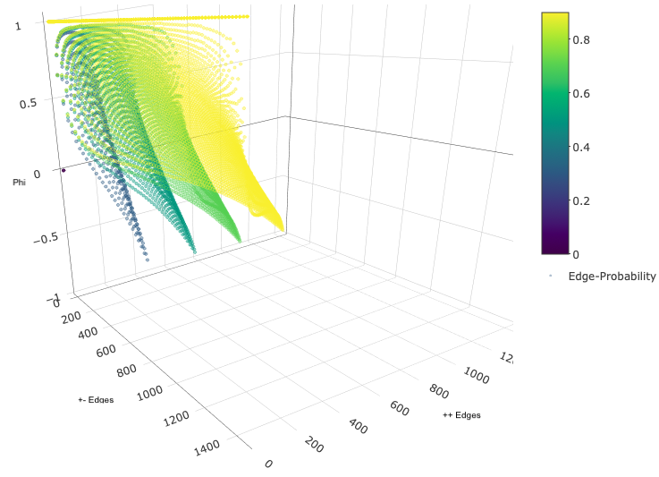
Figure 2. Maximum $\phi$ under the Erdős-Rényyi model: Number of edges per configuration $++,+-$ vs. $\phi$ and the sampling probability. Networks in yellow indicate higher density (edge-probability). Higher MSCC is achieved for networks with higher proportion of edges labeled $++$ than $+-$. The yellow line is parallel to the ’++’ axis

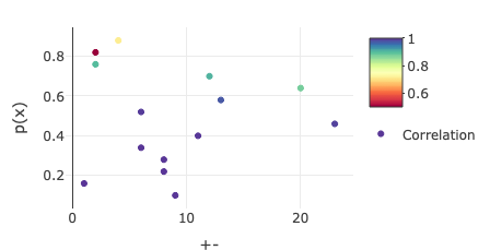
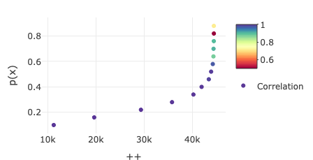
Figure 3. Maximum correlation for the GF model .

$p_{2}=0.4$ spacespacespacespacespacespacespacespacespacespace $p_{2}=0.5$

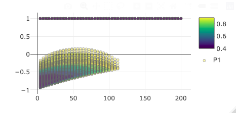
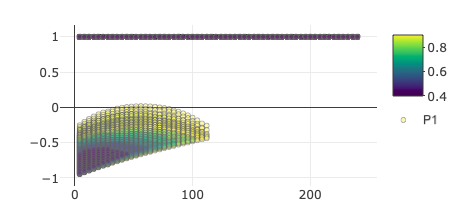
$p_{2}=0.6$ spacespacespacespacespacespacespacespacespacespace $p_{2}=0.7$

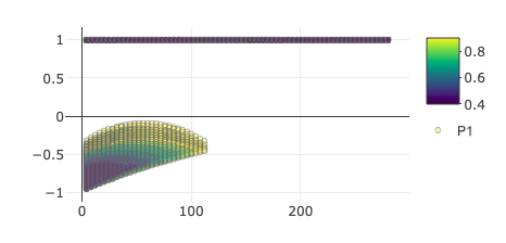
Figure 4. Maximum correlation under $2\times 2$ SBM (undirected). Horizontal axis $=\#$ of $++$ edges. Subplots: $p_{1}$ for $p_{2}=\{0.4,0.5,0.6,0.7\}$

In this experiment we evaluate our framework to perform goodness-of-fit based on the probabilities from Theorem 4. We fitted several real world datasets using the the Stochastic Block Model (SBM) (Holland et al., 1983) model for varying numbers of blocks. A summary of the characteristics of each dataset is presented in Table 1.

Table 1. Real Network Characteristics

Name	Nodes	Edges	Attribute (+)	Ref
adjnoun	109	11881	3564	(Newman, 2006)
dolphins	51	2601	770	(Lusseau et al., 2003)
polbooks	103	10609	3180	(boo, )
football	113	12769	3800	(Girvan and Newman, 2002)
lesmis	74	5476	1642	(Knuth, 1993)

Figure 1 shows the result of this analysis where the horizontal axis correspond to the various choices of the number of blocks and the vertical axis, the probability of representing the reference network. As we can see there, each network has a different optimal choice of $K$. For instance, the lesmis dataset has optimal $K=4$. Most of the datasets (all except football) have high probability of representing the reference graph even with a small value of $K$. The results in the figure also show that larger values of $K$ are less likely to represent the target network, which is obviously the case. The benefit of our work is to provide the tool to identify the conditions (in terms of the model probabilities) for the representation of the correlation of graphs with node attributes with the only constraint that the model belongs to the class of models $\mathcal{C}$. Ours is a non-asymptotic framework to understand the minimal size of a model (in terms of candidate edges and their probabilities) that can generate graphs with specific attribute correlations.

4.2. Simulations and Evaluation of Models

We evaluate empirically the values for maximum correlation that can be modeled under the GF and SBM models (additional experiments appear in the Appendix).

Figure 4 shows the maximum correlation as a function of the edge probability of SBM. Notice that since in SBM the parameters is a matrix, the maximum correlation corresponds to a spectrum of values that reflect how the parameters interact. Namely, for a $2\times 2$ SBM model with parameters $\Theta=\begin{bmatrix}p_{1}&p_{2}\\ p_{3}&p_{4}\end{bmatrix}$ $p_{1}$ and $p_{4}$ has an indirect impact on the maximum correlation achievable, e.g, values of the edge probability of $0.4$ can lead to a maximum correlation of $1$. On the other hand, $p_{2}$ and $p_{3}$ have a more direct impact on the maximum correlation and only large values of $p_{2},p_{3}$ can lead to a maximum correlation of $1$. This is somewhat counter-intuitive but could be explained from the point of view that a within cluster connectivity of $0.4$ may be sufficient to achieve the largest possible correlation.

Figure 3, presents the results for attributed graphs sampled from the graph frequency (GF) model. For the case of the analysis of edge probabilities we used the same parameters used in Cai et al. (2016): $\check{\alpha}=0.5$, $\check{\beta}=1$, $\check{\gamma}=3$ for the three-parameter generalized beta process that defines the edge-probabilities. As in Cai et al. (2016), we stop the process at $2000$ iterations and binarize the graphs. To make comparison fair, we use a number of nodes $N=1600$ and we study the effect of the likelihood among the number of $\beta_{1}$ and $\beta_{2}$ on the correlation. Notice that the monotonicity remains despite the complexity of the model.

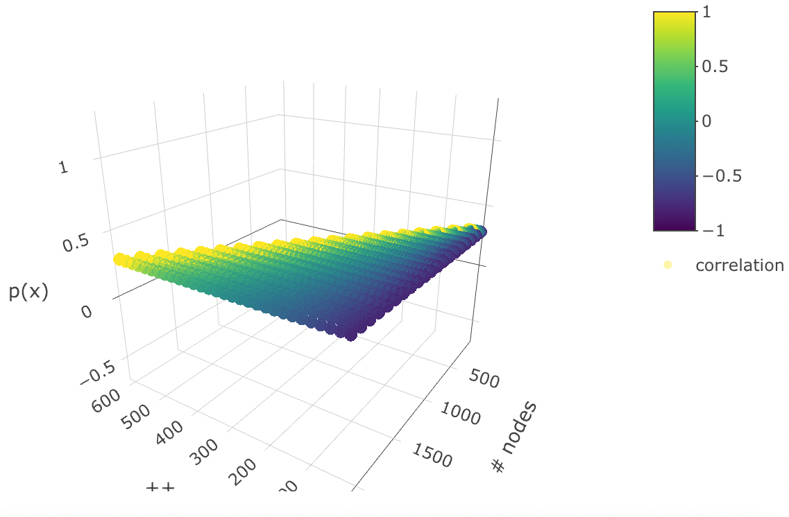
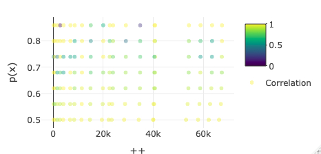
Figure 5. Effect of time for: left: the ER model right: GF model

Finally, Figure 5 shows the results of the effect of the number of nodes on the correlation. we explore the effect of $N$ for the GF model for the same $N$ in the range $[100,2000]$ with step size of $100$. We choose to plot a two-dimensional representation of the effect of $\beta_{1}$ on the maximum correlation because the maximum correlation does not define a clearly separated section of the graph space. This is due to both the complexity of the GF model and the non-trivial relation of the attribute marginal. Notice that due to the binarization the range of density of the nodes is wider than for the $ER$ model. Likewise, we show the case for the ER model with the same parameters, except for $N$, on the left sub-plot. We varied $N$ in the range $[100,2000]$ with step size of $100$. For the ER model we plot a three dimensional representation of the number of nodes, the number of $\beta_{1}$ edges, the attribute probability $p(X)$, and the effect on the maximum correlation (color-coded).

Figure 2 in the Appendix shows the maximum correlation as a function of the edge probability of the ER model as an additional illustrative example. This evaluation shows two important insights obtained from our theoretical framework. First the values of the correlations along $\beta_{1}$ values are monotonically increasing. Second, the maximum correlation of node attributes becomes more restricted as the value of the structural parameter $\Theta_{ER}=[p(x),N]$ increases. Notice that for this experiment we varied p(x) for $N=1600$. We also studied the effect over $N$ as shown later in this section.

5. Related Work

Prior work on models for attributed-graphs include (Bothorel et al., 2015; Silva et al., 2012; Kolar et al., 2014). Goodness-of-fit measures for graphs are a thriving area of research (Yang et al. (2018); Leppälä et al. (2017); Chen and Onnela (2019) etc.). However, goodness-of-fit for labeled graphs is less explored (Eswaran et al. (2019); Adriaens et al. (2020). To the best of our knowledge this problem has not been fully addressed in other works most of which rely on traditional metrics such as $r^{2}$ (Dimitriadis et al. (2020)). We define “characteristics” w.r.t the parameters such that both structure and node-attributes are captured simultaneously, as opposed to separately through traditional metrics.

Our work is related to the threshold phenomena in random graphs (Mossel et al. (2018, 2014); Kalai and Mossel (2015); Deshpande et al. (2018). The closest work to ours is (Mossel et al., 2018) which presented a solution to the clustering problem originally proposed by Decelle et al. (2011), namely, the Threshold Conjecture. However, the labels used in (Mossel et al., 2018) correspond to the block assignment of SBM - thus a clustering problem pertaining to the graph structure. Unlike this problem, ours considers labels drawn from a Bernoulli distribution and may define highly non-symmetric states that are fitted for the marginal distribution of node attributes that have little or no relation to the block community structure - thus ours is a sampling problem. Earlier threshold results for Boolean functions in graphs with symmetry, influence, and pivotality were reported by (Kalai and Safra, 2006).

The mean square contingency coefficient or $\phi$-coefficient is a measure of association between two binary variables. El-Sanhury and Davenport (Ernest C. Davenport and El-Sanhurry, 1991) proved the maximum values for $\phi$ in the case of a constant contingency table. However, this is not directly applicable to our analysis because the table in our case comes from random graphs. Thus, ours is a generalization of this work for the case of tables derived from random graphs.

6. Discussion and Conclusion

In this paper, we presented both sampling guarantees of a general class $\mathcal{C}$ of probabilistic generative models and a framework for sampling graph structure and node-attributes. Specifically, we introduced: the maximal marginal-error associated with the structural and attribute margins of the model and, an information-theoretical and probabilistic guarantee for a general class of models $\mathcal{C}$ equivalent to a possibly sparse parametric matrix. We also provided examples of the applicability of the analysis and an example of the probability of sample graphs (with specific auto-correlation) vs. the size of model in terms of its candidate edges. Our framework is focused on the assumption of sampling-agnostic exchangeability of structure and exchangeability preservation.

The main challenge we aimed to solve was assessing the correlation preservation of a model because preserving structure and attribute distribution can be done with existing Method of Moments and other statistical tools. Extensions to multiple-labeled graphs is not straightforward because the thresholds of each specific family of distributions may be considered.

Our work facilitates an understanding of characteristics of a generative model of node-attributed graphs and can be applied to hypothesis testing. It seeks to understand what type of data can be represented with a model using our probabilistic analysis. It can be used to reduce computational costs for model selection, network hypothesis testing, and among other possible applications (Asta and Shalizi, 2015).

Identifying theoretical constraints in probabilistic models of networks is relevant to the machine learning community because a thorough understanding of representation constraints in random graphs can help research communities determine which models are usable, for instance via hypothesis test – this is highly relevant to such varied domains as relational learning, collaborative filtering, graph mining, etc., where evaluation of graph models are useful.

7. Appendix

7.1. Additional Details of the Proofs of the Theorems

Proof.

Lemma 3 Since the unique probabilities $\pi_{j}\in\mathbf{U}$ are Bernoulli-distributed, the number of edges to sample $y_{j}\sim Bin(n_{j},\pi_{j})$ are binomial-distributed. Consider the tail bounds of the binomial distribution (Arriata and Gordon, 1989) :

$$\begin{array}[]{l}Pr(X\leq k;n,p)\leq e^{\left(-nD_{KL}\left(\frac{k}{n}||p\right)\right)}\mbox{ if }0<\frac{k}{n}<p;\\ Pr(X\geq k;n,p)\leq e^{\left(-nD_{KL}\left(\frac{k}{n}||p\right)\right)}\mbox{ if }p<\frac{k}{n}<1.\\ \end{array}\vspace{-0.5em}$$

Then,

$$\footnotesize{\begin{array}[]{l}Pr(y_{j}\leq N_{1j}+N_{3_{j}};n_{j},\pi_{j})\leq e^{\left(-n_{j}D_{KL}\left(r_{j}||\pi_{j}\right)\right)}\mbox{ if }0<r_{j}<\pi_{j};\\ Pr(y_{j}\geq N_{1j}+N_{3_{j}};n_{j},\pi_{j})\leq e^{\left(-n_{j}D_{KL}\left(r_{j}||\pi_{j}\right)\right)}\mbox{ if }\pi_{j}<r_{j}<1.\\ \end{array}}$$

To find $\exp(-w)<10^{-10}$ consider $-w<-10\log{10}\Rightarrow w>23.03$. Then

$$\left\{\begin{array}[]{l}Pr(y_{j}>N_{1j}+N_{3_{j}};n_{j},\pi_{j})>1-10^{-10},\mbox{ if }\left(n_{j}D_{KL}\left(r_{j}||\pi_{j}\right)\right)>23.03\mbox{ and }0<r_{j}<\pi_{j};\\ Pr(y_{j}<N_{1j}+N_{3_{j}};n_{j},\pi_{j})>1-10^{-10},\mbox{ if }\left(n_{j}D_{KL}\left(r_{j}||\pi_{j}\right)\right)>23.03\mbox{ and }\pi_{j}<r_{j}<1.\\ \end{array}\right.\vspace{-1.7em}$$

∎

Proof.

Lemma 6 Consider the function $\rho:\mathcal{U}\rightarrow[-1,1]$ defined in Equation (3). This function is monotonically increasing along $\beta_{1}$ because

$$\frac{\partial\rho}{\partial\beta_{1}}=\frac{4(\beta_{1}+1)\beta_{3}+2(\beta_{1}-1)^{2}-6\beta_{3}^{2}}{((\beta_{1}-\beta_{3})^{2}-1)^{2}}\geq 0.$$

Likewise, this function is monotonically increasing along $\beta_{3}$ because

$$\frac{\partial\rho}{\partial\beta_{3}}=\frac{4(\beta_{3}+1)\beta_{1}+2(\beta_{3}-1)^{2}-6\beta_{1}^{2}}{((\beta_{3}-\beta_{1})^{2}-1)^{2}}\geq 0.$$

Then, by Remark 5, after considering the dimensions $x_{1},x_{2}$ as $\beta_{1},\beta_{3}$, it follows that for $\vec{\beta}\preceq\vec{\beta}^{\prime}\Rightarrow\rho(\vec{\beta})\leq\rho(\vec{\beta}^{\prime})$. ∎

Proof.

Lemma 7
The conditions $|\beta_{1}-\tilde{\beta}_{1}|<\epsilon_{1}\mbox{ and }|\beta_{3}-\tilde{\beta}_{3}|<\epsilon_{3}$ are equivalent to $\beta_{1}-\epsilon_{1}<\tilde{\beta}_{1}<\beta_{1}+\epsilon_{1}\mbox{ and }\beta_{3}-\epsilon_{3}<\tilde{\beta}_{3}<\beta_{3}+\epsilon_{3}$. Thus, the solution is defined by the values $\tilde{\beta}_{1},\tilde{\beta}_{3}$ that maximize the difference of the correlations in the squared region $(\beta_{1},\beta_{3})+[-\epsilon_{1},\epsilon_{1}]\times[-\epsilon_{3},\epsilon_{3}]$.

From Lemma 6, we know that the correlation is monotonically increasing with respect to projections in each dimension $\beta_{1},\beta_{3}$. Then

$$\epsilon =\max(|\rho_{IN}-\rho_{OUT}|)=\max(|\rho(\tilde{\beta}_{1},\tilde{\beta}_{3})-\rho(\beta_{1},\beta_{3})|)$$

$$=\max(\rho(\beta_{1}+\epsilon_{1},\beta_{3}+\epsilon_{3})-\rho(\beta_{1},\beta_{3}),-\rho(\beta_{1}-\epsilon_{1},\beta_{3}-\epsilon_{3})+\rho(\beta_{1},\beta_{3})).$$

Thus, for values of $\rho(\tilde{\beta}_{1},\tilde{\beta}_{3})$ that oversample $\rho_{IN}$ we can use the expression:

$$\rho(\beta_{1}+\epsilon_{1},\beta_{3}+\epsilon_{3}) -\rho(\beta_{1},\beta_{3})$$

$$=\frac{(\beta_{3}+\epsilon_{3})-\left(\beta_{3}+\epsilon_{3}+\frac{1-\beta_{1}-\epsilon_{1}-\beta_{3}-\epsilon_{3}}{2}\right)^{2}}{(\beta_{3}+\epsilon_{3}+(1-\beta_{1}-\epsilon_{1}-\beta_{3}-\epsilon_{3})/2)(1-(\beta_{3}+\epsilon_{3}+(1-\beta_{1}-\epsilon_{1}-\beta_{3}-\epsilon_{3}))/2)}$$

$$\quad-\frac{(\beta_{3})-\left(\beta_{3}+\frac{1-\beta_{1}-\beta_{3}}{2}\right)^{2}}{(\beta_{3}+(1-\beta_{1}-\beta_{3})/2)(1-(\beta_{3}+(1-\beta_{1}-\beta_{3}))/2)}.$$

Therefore,

$$\epsilon =\frac{\beta_{3}-(p+\Delta p)^{2}}{(p+\Delta p)(1-p-\Delta p)}-\frac{\beta_{3}-p^{2}}{p(1-p)},$$

where $\Delta p=\epsilon_{3}+\frac{-\epsilon_{1}-\epsilon_{3}}{2}$.

∎

Proof.

Theorem 4

Consider the case of a tight bound on $\vec{\beta}$ and let $\beta_{i}$ be each entry of $\vec{\beta}$ (i.e., derived from the data) and let $\tilde{\beta}_{i}$ be associated to the output/sampled graph. By lemma 7 there is an $\epsilon$:

$$|\beta_{1}-\tilde{\beta}_{1}|<\epsilon_{1}\mbox{ and }|\beta_{2}-\tilde{\beta}_{2}|<\epsilon_{2}\Rightarrow|\rho_{IN}-\rho_{OUT}|<\epsilon,$$

Consider $\beta_{i}$ constant. Replacing the definitions of the ratios in $|\beta_{i}-\tilde{\beta}_{i}|<\epsilon_{i}$ gives us $\left|\beta_{i}-\frac{\sum_{j}^{\kappa}\chi_{ij}}{\sum_{j}^{\kappa}y_{j}}\right|<\epsilon_{i}$.

Notice that $\chi$ and $y_{j}$ are not independent and $\chi_{ij}<y_{j}$. In fact, $\chi_{ij}<N_{ij}$. Now the value of $\chi$ can be deterministic or probabilistic. Consider the deterministic case (we will consider the probabilistic case in Thm 1):

$$\frac{\sum_{j}^{\kappa}\chi_{ij}}{\beta_{i}+\epsilon_{i}}<\sum_{j}^{\kappa}y_{j}<\frac{\sum_{j}^{\kappa}\chi_{ij}}{\beta_{i}-\epsilon_{i}},$$

or

$$Pr\left(\sum_{j}^{\kappa}y_{j}<\frac{\sum_{j}^{\kappa}\chi_{ij}}{\beta_{i}-\epsilon_{i}}\right)-Pr\left(\sum_{j}^{\kappa}y_{j}<\frac{\sum_{j}^{\kappa}\chi_{ij}}{\beta_{i}+\epsilon_{i}}\right).$$

Let $X=\sum_{j}^{\kappa}y_{j}$, then $Pr\left(X<a\right)-Pr\left(X<b\right)>1-\delta$ can be written as $\left(Pr\left(X>a\right)+Pr\left(X<b\right)\right)<\delta$. Alternately, considering $Pr\left(X>a\right)<\delta_{1}$ and $Pr\left(X<b\right)<\delta_{2}$, then

$$\left(Pr\left(X>a\right)+Pr\left(X<b\right)\right)<\delta_{1}+\delta_{2}.$$

Consider $a=(1+\xi)\mu$ for $\mu=E[X]$ and $0<\xi<1$, then by multiplicative Chernoff bound:

$$Pr\left(X>a\right)\leq e^{-\frac{\xi^{2}\mu}{3}}=e^{-\frac{{({a-\mu})}^{2}}{3\mu}},$$

where the equality follows by $\xi=\frac{a-\mu}{\mu}$. Consider $b=(1-\xi^{\prime})\mu$ for $\mu=E[X]$ and $0<\xi^{\prime}<1$, then, by the same bound:

$$Pr\left(X<b\right)\leq e^{-\frac{\xi^{\prime 2}\mu}{2}}=e^{-\frac{{({\mu}-b)}^{2}}{2\mu}},$$

— recall $\left(Pr\left(X>a\right)+Pr\left(X<b\right)\right)<\delta_{1}+\delta_{2}$ – Then: $Pr(|\beta_{i}-\tilde{\beta}_{i}|<\epsilon_{i})>1-(e^{-\frac{{({a-\mu})}^{2}}{3\mu}}+e^{-\frac{{({\mu}-b)}^{2}}{2\mu}})$ or equivalently:

$$Pr(|\beta_{i}-\tilde{\beta}_{i}|<\epsilon_{i})>1-\left(e^{-\frac{{\left({\frac{\sum_{j}^{\kappa}\chi_{ij}}{\beta_{i}-\epsilon_{i}}-\mu}\right)}^{2}}{3\mu}}+e^{-\frac{{\left({\mu}-\frac{\sum_{j}^{\kappa}\chi_{ij}}{\beta_{i}+\epsilon_{i}}\right)}^{2}}{2\mu}}\right).$$

Thus, $P(|\rho_{IN}-\rho_{OUT}|<\epsilon)>1-\delta$ for $\delta=\sum_{i=1}^{2}\tau_{i}-\prod_{i=1}^{2}\tau_{i}$ and $\tau_{i}=\exp{\left(-{{\left({\frac{\sum_{j}^{\kappa}\chi_{ij}}{\beta_{i}-\epsilon_{i}}-\mu}\right)}^{2}}/{3\mu}\right)}+\exp{\left(-{{\left({\mu}-\frac{\sum_{j}^{\kappa}\chi_{ij}}{\beta_{i}+\epsilon_{i}}\right)}^{2}}/{2\mu}\right)}$. ∎

Theorem 1 (Correlation Recovery - Random $\rho_{IN}$).

Let $\chi_{ij}$ be the number of edges sampled by $\mathcal{S}$ per edge-label $\psi_{i}$ and parameter $\pi_{j}$ and $\mu=\sum_{j}^{\kappa}y_{j}$ for $y_{j}\sim Bin(n_{j},\pi_{j})$ (number of edges to sample). Then, for any $\mathcal{M}$ and $\mathcal{S}$ and small $\delta,\epsilon_{1},\epsilon_{3}>0$, the bound of the difference between the target correlation $\rho_{IN}$ and the correlation of the sampled graph $\rho_{OUT}$, as per the limited range of edges sampled $\chi_{ij}$ has probability

(5) $$P(|\rho_{IN}-\rho_{OUT}|<\epsilon)>1-\delta,$$

for $\delta=\sum_{i=1}^{2}\tau_{i}+\prod_{i=1}^{2}\tau_{i}$,
where $\tau_{i}=\exp{\left(-{{\left({\mathbbm{E}\left[(\beta_{i}-\epsilon_{i})^{-1}{\sum_{j}^{\kappa}\chi_{ij}}\right]-\mu}\right)}^{2}}/{3\mu}\right)}+\exp{\left(-{{\left({\mu}-\mathbbm{E}\left[(\beta_{i}+\epsilon_{i})^{-1}{\sum_{j}^{\kappa}\chi_{ij}}\right]\right)}^{2}}/{2\mu}\right)}$
and $\epsilon=\frac{\beta_{3}-(p+\Delta p)^{2}}{(p+\Delta p)(1-p-\Delta p)}-\frac{\beta_{3}-p^{2}}{p(1-p)}$, where $p=\beta_{3}+\frac{1-\beta_{1}-\beta_{3}}{2}$ and $\Delta p=\epsilon_{3}+\frac{-\epsilon_{1}-\epsilon_{3}}{2}$.

Theorem 1 describes the number of edges per parameter and edge-label samples required to maximize the probability of obtaining a target autocorrelation distribution.

Notice that $\rho$ in this theorem is not assumed to be a constant but a random variable with a distribution. However, sampling of edges is still done by conditioning on attributes and then defining $\mathbf{U}$, $N,\psi,\beta$ and indices $\mathcal{T}$. This value is similar to the one obtained for Theorem 4, except that the value in Theorem 1 is in expectation and is only valid for values of the variables that are concave around $\mu$ (limited range of $\chi_{ij}$). This condition does not affect the generality of the theorem since the proof includes the relations in terms of the sampling distributions (Further details in the Appendix) required to maximize the probability of obtaining a target autocorrelation distribution. $P(U)$) that describe the behavior of the correlation.

Proof.

Theorem 1

The following is the full proof. As in the previous case, consider the case of a tight bound on $\vec{\beta}$ and let $\beta_{i}$ be each entry of $\vec{\beta}$ (i.e., derived from the data) and let $\tilde{\beta}_{i}$ be associated to the output/sampled graph.

$$|\beta_{1}-\tilde{\beta}_{1}|<\epsilon_{1}\mbox{ and }|\beta_{2}-\tilde{\beta}_{2}|<\epsilon_{2}\Rightarrow|\rho_{IN}-\rho_{OUT}|<\epsilon.$$

Consider $\beta_{i}$ to be random and recall:

$$Pr\left(\sum_{j}^{\kappa}y_{j}<\frac{\sum_{j}^{\kappa}\chi_{ij}}{\beta_{i}-\epsilon_{i}}\right)-Pr\left(\sum_{j}^{\kappa}y_{j}<\frac{\sum_{j}^{\kappa}\chi_{ij}}{\beta_{i}+\epsilon_{i}}\right).$$

Let $X=\sum_{j}^{\kappa}y_{j}$, $U=\frac{\sum_{j}^{\kappa}\chi_{ij}}{\beta_{i}-\epsilon_{i}}$, and $V=\frac{\sum_{j}^{\kappa}\chi_{ij}}{\beta_{i}+\epsilon_{i}}$, we can rewrite the above as

$$Pr\left(X<U\right)-Pr\left(X<V\right);$$

$$Pr\left(X<U\right)=\sum_{u}Pr(X<U|U=u)Pr(U=u).$$

Since

$$Pr\left(X<b\right)\leq e^{-\frac{\xi^{\prime 2}\mu}{2}}=e^{-\frac{{({\mu}-b)}^{2}}{2\mu}},$$

and

$$Pr\left(X>a\right)\leq e^{-\frac{\xi^{2}\mu}{3}}=e^{-\frac{{({a-\mu})}^{2}}{3\mu}},$$

we have

$$Pr\left(X<V\right)\leq\sum_{v}e^{-\frac{{({\mu}-v)}^{2}}{2\mu}}Pr(V=v);$$

$$Pr\left(X>U\right)\leq\sum_{u}e^{-\frac{{({u-\mu})}^{2}}{3\mu}}Pr(U=u).$$

Notice that $U$ and $V$ have inverse distributions:

$$Pr\left(X<V\right)\leq\mathbbm{E}_{V}\left[e^{-\frac{{({\mu}-V)}^{2}}{2\mu}}\right];$$

$$Pr\left(X>U\right)\leq\mathbbm{E}_{U}\left[e^{-\frac{{({U-\mu})}^{2}}{3\mu}}\right].$$

Since Jensen’s inequality is applicable on arbitrary intervals of a partially convex function as long as the function is Borel measurable, we apply the inequality to the convex region of the Gaussian density defined in $\mu\pm\sigma$ (can be determined via inflection points criteria). In a few words, the functions above are concave around $\mu$. Thus, by Jensen’s inequality:

$$Pr\left(X<V\right)<e^{-\frac{{({\mu}-\mathbbm{E}[{V}])}^{2}}{2\mu}};$$

$$Pr\left(X>U\right)<e^{-\frac{{({\mathbbm{E}[{U}]-\mu})}^{2}}{3\mu}}.$$

Following the same steps than the previous theorem, it is easy to see that

$$P(|\rho_{IN}-\rho_{OUT}|<\epsilon)>1-\sum_{i=1}^{2}\tau_{i}+\prod_{i=1}^{2}\tau_{i},$$

where $\tau_{i}=\exp{\left(-{{\left({\mathbbm{E}\left[\frac{\sum_{j}^{\kappa}\chi_{ij}}{\beta_{i}-\epsilon_{i}}\right]-\mu}\right)}^{2}}/{3\mu}\right)}+\exp{\left(-{{\left({\mu}-\mathbbm{E}\left[\frac{\sum_{j}^{\kappa}\chi_{ij}}{\beta_{i}+\epsilon_{i}}\right]\right)}^{2}}/{2\mu}\right)}$
and $\epsilon=\frac{\beta_{1}\beta_{3}-\gamma^{2}}{(\beta_{1}+\gamma)(\beta_{3}+\gamma)}-\frac{\beta_{1}^{{}^{\prime}}\beta_{3}^{{}^{\prime}}-{\gamma^{2}}^{{}^{\prime}}}{(\beta_{1}^{{}^{\prime}}+\gamma^{{}^{\prime}})(\beta_{3}^{{}^{\prime}}+\gamma^{{}^{\prime}})}$, where $\gamma=\beta_{2}/2$ and $\gamma^{{}^{\prime}}=\beta_{2}^{{}^{\prime}}/2.$ ∎

7.2. Additional Experiment Figures

References

- [1] Social organizational network analysis software. URL http://www.orgnet.com/.
- Adriaens et al. [2020] Florian Adriaens, Alexandru Mara, Jefrey Lijffijt, and Tijl De Bie. Block-approximated exponential random graphs. In 2020 IEEE 7th International Conference on Data Science and Advanced Analytics (DSAA), pages 70–80. IEEE, 2020.
- Ahmed and Xing [2009] Amr Ahmed and Eric P. Xing. Recovering time-varying networks of dependencies in social and biological studies. Proceedings of the National Academy of Sciences, 106(29):11878–11883, 2009.
- Asta and Shalizi [2015] Dena Marie Asta and Cosma Rohilla Shalizi. Geometric network comparisons. In UAI, 2015.
- Bansal et al. [2004] Nikhil Bansal, Avrim Blum, and Shuchi Chawla. Correlation clustering. Mach. Learn., 56(1-3):89–113, June 2004. ISSN 0885-6125. doi: 10.1023/B:MACH.0000033116.57574.95. URL https://doi.org/10.1023/B:MACH.0000033116.57574.95.
- Barabasi and Albert [1999] A. Barabasi and R. Albert. Emergence of scaling in random networks. Science, 286:509–512, 1999.
- Bothorel et al. [2015] Cecile Bothorel, Juan David Cruz, Matteo Magnani, and Barbora Micenkova. Clustering attributed graphs: Models, measures and methods. Network Science, 3(3):408–444, 2015.
- Cai et al. [2016] Diana Cai, Trevor Campbell, and Tamara Broderick. Edge-exchangeable graphs and sparsity. In D. D. Lee, M. Sugiyama, U. V. Luxburg, I. Guyon, and R. Garnett, editors, Advances in Neural Information Processing Systems 29, pages 4249–4257. Curran Associates, Inc., 2016.
- Chen and Onnela [2019] Sixing Chen and Jukka-Pekka Onnela. A bootstrap method for goodness of fit and model selection with a single observed network. Scientific reports, 9(1):1–12, 2019.
- Cramer [1946] Harold Cramer. Mathematical methods of statistics, princeton univ. Press, Princeton, NJ, 1946.
- Crane and Dempsey [2016] Harry Crane and Walter Dempsey. Edge exchangeable models for network data. arXiv preprint arXiv:1603.04571, 2016.
- de Solla Price [1976] Derek de Solla Price. A general theory of bibliometric and other cumulative advantage processes. Journal of the Association for Information Science and Technology, 27(5):292–306, 1976.
- Decelle et al. [2011] Aurelien Decelle, Florent Krzakala, Cristopher Moore, and Lenka Zdeborová. Asymptotic analysis of the stochastic block model for modular networks and its algorithmic applications. Phys. Rev. E, 84:066106, Dec 2011.
- Deshpande et al. [2018] Yash Deshpande, Subhabrata Sen, Andrea Montanari, and Elchanan Mossel. Contextual stochastic block models. Advances in Neural Information Processing Systems, 31, 2018.
- Dimitriadis et al. [2020] Ilias Dimitriadis, Marinos Poiitis, Christos Faloutsos, and Athena Vakali. Triage: Temporal twitter attribute graph patterns. In Proceedings of the 10th International Conference on Web Intelligence, Mining and Semantics, pages 44–53, 2020.
- [16] N. El-Sanhury and E Davenport. Phi/phimax: Review and synthesis educational and psychological measurement. Educational and Psychological Measurement, 51(4):821–828.
- Ernest C. Davenport and El-Sanhurry [1991] Jr. Ernest C. Davenport and Nader A. El-Sanhurry. Phi/phimax: Review and synthesis. Educational and Psychological Measurement, 51(4):821–828, 1991.
- Eswaran et al. [2019] Dhivya Eswaran, Reihaneh Rabbany, Arthur Dubrawski, and Christos Faloutsos. Social-affiliation networks: Patterns and the soar model. In Machine Learning and Knowledge Discovery in Databases: European Conference, ECML PKDD 2018, Dublin, Ireland, September 10–14, 2018, Proceedings, Part II, volume 11052, page 105. Springer, 2019.
- Girvan and Newman [2002] Michelle Girvan and Mark EJ Newman. Community structure in social and biological networks. Proceedings of the national academy of sciences, 99(12):7821–7826, 2002.
- Holland et al. [1983] Paul W Holland, Kathryn Blackmond Laskey, and Samuel Leinhardt. Stochastic blockmodels: First steps. Social networks, 5(2):109–137, 1983.
- Holme and Kim [2002] Petter Holme and Beom Jun Kim. Growing scale-free networks with tunable clustering. Physical review E, 65(2):026107, 2002.
- Jeong et al. [2000] H. Jeong, B. Tombor, R. Albert, Z. N. Oltvai, and A. L. Barabasi. The large-scale organization of metabolic networks. Nature, 407(6804):651–654, 10 2000.
- Kalai and Mossel [2015] Gil Kalai and Elchanan Mossel. Sharp thresholds for monotone non-boolean functions and social choice theory. Mathematics of Operations Research, 40(4):915–925, 2015.
- Kalai and Safra [2006] Gil Kalai and Shmuel Safra. Perspectives from mathematics, computer science, and economics. Computational complexity and statistical physics, page 25, 2006.
- Kim and Leskovec [2010] Myunghwan Kim and Jure Leskovec. Multiplicative attribute graph model of real-world networks. In Algorithms and Models for the Web-Graph, volume 6516 of Lecture Notes in Computer Science, pages 62–73, 2010. ISBN 978-3-642-18008-8.
- Knuth [1993] Donald E Knuth. The Stanford GraphBase: a platform for combinatorial computing. Addison-Wesley, 1993.
- Kolar et al. [2014] Mladen Kolar, Han Liu, and Eric P. Xing. Graph estimation from multi-attribute data. J. Mach. Learn. Res., 15(1):1713–1750, January 2014. ISSN 1532-4435.
- Leppälä et al. [2017] Kalle Leppälä, Svend V Nielsen, and Thomas Mailund. admixturegraph: an r package for admixture graph manipulation and fitting. Bioinformatics, 33(11):1738–1740, 2017.
- Lusseau et al. [2003] David Lusseau, Karsten Schneider, Oliver J Boisseau, Patti Haase, Elisabeth Slooten, and Steve M Dawson. The bottlenose dolphin community of doubtful sound features a large proportion of long-lasting associations. Behavioral Ecology and Sociobiology, 54(4):396–405, 2003.
- Mossel et al. [2014] Elchanan Mossel, Joe Neeman, and Allan Sly. Consistency thresholds for binary symmetric block models. arXiv preprint arXiv:1407.1591, 2014.
- Mossel et al. [2018] Elchanan Mossel, Joe Neeman, and Allan Sly. A proof of the block model threshold conjecture. Combinatorica, 38(3):665–708, 2018.
- Newman [2006] Mark EJ Newman. Finding community structure in networks using the eigenvectors of matrices. Physical review E, 74(3):036104, 2006.
- Pfeiffer III et al. [2014] J. J. Pfeiffer III, S. Moreno, T. La Fond, J. Neville, and B. Gallagher. Attributed graph models: Modeling network structure with correlated attributes. In Proceedings of the Twenty-Third International Conference on World Wide Web, WWW ’14, pages 831–842, 2014. ISBN 978-1-4503-2744-2.
- Powers [2020] David MW Powers. Evaluation: from precision, recall and f-measure to roc, informedness, markedness and correlation. arXiv preprint arXiv:2010.16061, 2020.
- Psorakis et al. [2012] Ioannis Psorakis, Stephen J. Roberts, Iead Rezek, and Ben C. Sheldon. Inferring social network structure in ecological systems from spatio-temporal data streams. Journal of The Royal Society Interface, 2012. ISSN 1742-5689.
- Rényi and Erdős [1959] A Rényi and P Erdős. On random graph. Publicationes Mathematicate, 6:290–297, 1959.
- Shalizi and Rinaldo [2013] Cosma Rohilla Shalizi and Alessandro Rinaldo. Consistency under sampling of exponential random graph models. Ann. Statist., 41(2):508–535, 04 2013.
- Shore and Lubin [2015] Jesse Shore and Benjamin Lubin. Spectral goodness of fit for network models. Social Networks, 43:16–27, 2015. ISSN 0378-8733.
- Silva et al. [2012] Arlei Silva, Wagner Meira, Jr., and Mohammed J. Zaki. Mining attribute-structure correlated patterns in large attributed graphs. Proc. VLDB Endow., 5(5):466–477, January 2012. ISSN 2150-8097.
- Spyropoulou et al. [2014] Eirini Spyropoulou, Tijl De Bie, and Mario Boley. Interesting pattern mining in multi-relational data. Data Mining and Knowledge Discovery, 28(3):808–849, 2014. ISSN 1384-5810.
- Weckbecker et al. [2022] Moritz Weckbecker, Wenkai Xu, and Gesine Reinert. On rkhs choices for assessing graph generators via kernel stein statistics. arXiv preprint arXiv:2210.05746, 2022.
- Yang et al. [2018] Jiasen Yang, Qiang Liu, Vinayak Rao, and Jennifer Neville. Goodness-of-fit testing for discrete distributions via stein discrepancy. In Jennifer Dy and Andreas Krause, editors, Proceedings of the 35th International Conference on Machine Learning, volume 80 of Proceedings of Machine Learning Research, pages 5561–5570, 2018.
- Zhou and Nakhleh [2011] Wanding Zhou and Luay Nakhleh. Properties of metabolic graphs: Biological organization or representation artifacts? BMC Bioinformatics, 12(1):1–12, 2011. ISSN 1471-2105.
- Zhu [2020] Qiuming Zhu. On the performance of matthews correlation coefficient (mcc) for imbalanced dataset. Pattern Recognition Letters, 136:71–80, 2020.