Real and complexified configuration spaces for spherical 4-bar linkages
This note is a complete library of symbolic parametrized expressions for both real and complexified configuration spaces of a spherical 4-bar linkage. Building upon the previous work from Izmestiev (2016, Section 2), this library expands on the expressions by incorporating all four folding angles across all possible linkage length choices, along with the polynomial relation between diagonals (spherical arcs). Furthermore, a complete MATLAB app script He (2023) is included, enabling visualization and parametrization. The derivations are presented in a detailed manner, ensuring accessibility for researchers across diverse disciplines.
The spherical 4-bar linkage is an essential constituent of single-degree-of-freedom mechanisms that have held significant importance in engineering for over two centuries. By substituting each spherical linkage with a sectoral rigid panel and each joint with a rotational hinge, an analogous panel-hinge mechanism is obtained. Within the domain of origami engineering, such a mechanism is referred to as a degree-4 single-vertex rigid origami, which has garnered considerable attention in both theoretical and practical applications. Extensive literature exists on the theories and applications of the spherical 4-bar linkage or the degree-4 single-vertex rigid origami. This note specifically focuses on the theoretical aspects and provides comprehensive analytical calculations and examinations for all forms of algebraic analyses. We further refer to Chen and Chiang (1983) for the fourth-order synthesis on adjacent folding angles and analysis on the locus of the pole between the coupler and the fixed linkage; Gibson and Selig (1988a, b) for a series of results on the properties, singularities and reduction of the configuration space under different choices of linkage lengths; Khimshiashvili (2011) for a series of results on the moduli space, cross-ratio, generalized Heron polynomials that can calculate the area of the (spherical) quadrilateral, etc. In origami engineering, we refer to Waitukaitis and van Hecke (2016), Zimmermann and Stanković (2020), Foschi et al. (2022) for analytical calculation on a degree-4 vertex using spherical trigonometry under a case-by-case discussion.
In conjunction with these aforementioned contributions, the information provided in this note serves as a valuable handbook for engineers, architects, and mathematicians seeking parametrized symbolic expressions for configuring 4-bar linkage-based mechanisms.
1 Modelling
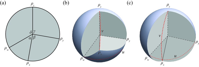
In this section we will set up the notation for a spherical 4-bar linkage, which is shown in Figure 1. We use to describe the magnitudes of sector angles and four folding angles to describe the configuration. means are equivalent if , which implies that we take and as the same rotational angle.
The tangents of half of the folding angles are defined as
| (1) |
is the one-point compactification of the real line, which ‘glues’ and to the same point. Moreover, in further algebraic discussions, and are the lengths of spherical diagonals.
Remark 1.
If considering the ‘stacking sequence’ of these linkages, it is also reasonable to require to be different from . This definition will make , which is called the two-point compactification of the real line.
First, we have the following proposition on the range of sector angles.
Proposition 1.
are the sector angles of a degree-4 single-vertex if and only if
| (2) |
Proof.
Necessity: Suppose we have a degree-4 single vertex,
| (3) |
are all spherical quadrilaterals, hence Equation (2) holds.
Sufficiency: Consider the four spherical triangles , , and when . should satisfy the following condition:
| (4) |
The sufficient condition for to be the sector angles of a degree-4 single-vertex is the range of and being non-empty, which means:
| (5) |
This leads to Equation (2). ∎
Next we will give the polynomial relation between:
-
[1]
adjacent rotational angles and ; and .
-
[2]
opposite rotational angles and .
-
[3]
lengths of diagonals and .
then conduct a detailed case-by-case discussion.
2 Relation between adjacent folding angles
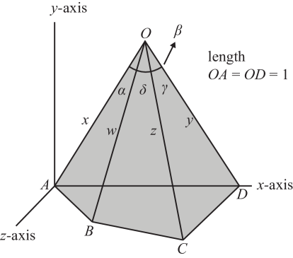
One method to derive the relation between adjacent folding angles is to build an Euclidean coordinate system, as shown in Figure 2. With the provided dimensions we could write the coordinates of and as:
Within triangle OBC we could get the relation between and :
The next step is to simplify the above equation to a polynomial equation on and , the result is:
We further simplify the above equation to the polynomial form below:
| (6) |
is the semi-perimeter of a spherical 4-bar linkage. Note that satisfy Proposition 1, and we allow in Equation (6).
Further we will classify Equation (6) based on the degree of degeneracy – how many of are zero (). From Proposition 1 we have:
We classify a spherical 4-bar linkage in the following way:
-
[1]
a square, if:
-
[2]
a rhombus, if:
-
[3]
a cross, if:
-
[4]
of type Miura I, if:
-
[5]
of type Miura II, if:
-
[6]
an isogram, if:
-
[7]
an anti-isogram, if:
-
[8]
a deltoid I, if:
-
[9]
an anti-deltoid I, if:
-
[10]
a deltoid II, if:
-
[11]
an anti-deltoid II, if:
-
[12]
of type conic I, if:
-
[13]
of type conic II, if:
-
[14]
of type conic III, if:
-
[15]
of type conic IV, if:
-
[16]
of type elliptic, if:
Further, if the following relation is satisfied:
We call this type orthodiagonal since the diagonals are orthogonal on the sphere (sum of the square of opposite arc lengths are equal), and we will analyze its special configuration space later.
Similarly, for the standard form on and , we have the following relation:
| (7) |
3 Relation between opposite folding angles
In terms of and , we could derive the relation between and from spherical trigonometry.
Next step is to transfer them to polynomials,
which leads to the simplified polynomial form on and below:
| (8) |
where
The identities listed in Proposition 3 would help to understand the symmetry of coefficients in Equation (8).
It is clear that and . Note that and can be separated if :
| (9) |
Equation (8) after a case-by-case study is:
-
[1]
square
-
[2]
rhombus
-
[3]
cross
-
[4]
Miura I
-
[5]
Miura II
-
[6]
isogram
-
[7]
anti-isogram
-
[8]
deltoid I
-
[9]
anti-deltoid I
-
[10]
deltoid II
-
[11]
anti-deltoid II
- [12]
-
[13]
conic II
-
[14]
conic III
-
[15]
conic IV
-
[16]
Elliptic. See Section 22 since the expression is not reduced.
4 Relation between the lengths of diagonals
The polynomial relation between the spherical lengths of diagonals and is also of interest to us and is actually used quite often.
For simplicity, we need to consider the relation between and without involving the folding angles. A great tool is called the spherical version of the Cayley-Menger determinant over the four points of a spherical 4-bar linkage. The condition for this linkage lying on a sphere is:
After full simplification, the result is an order 3 polynomial over and :
| (10) | ||||
where
Here we use two simple examples to show how to make use of Equation (10):
-
[1]
square
-
[2]
rhombus
An important conclusion below is derived from Equation (10):
Proposition 2.
There is a one-to-one correspondence between the two spherical 4-bar linkages below:
| (11) |
That is to say, for every spherical 4-bar linkage with sector angles and diagonal lengths , there is another spherical 4-bar linkage with sector angles and the same diagonal lengths . We say they are conjugate spherical 4-bar linkages.
Actually, from direct symbolic calculations with the helpful identities provided in Proposition 3 below, we could see that the coefficients preserve when switching a spherical 4-bar linkage to its conjugate.
5 Helpful identities and sign convention
In this section we will provide some helpful identities in the study of the above polynomial relations.
Proposition 3.
Some identities over and . Note that is the semi-perimeter.
-
[1]
-
[2]
-
[3]
-
[4]
-
[5]
-
[6]
-
[7]
-
[8]
-
[9]
When :
These identities also hold for all the permutations over .
We will also provide some conventions and notations used throughout this note:
| (12) |
At the end of this section we introduce the following important transformation called ‘switching a strip’:
Proposition 4.
One-to-one correspondence between two spherical quadrilaterals.
-
[1]
-
[2]
-
[3]
-
[4]
6 Post-examination, solutions at infinity
Generically, given a flex of we will have two solutions of from Equation (6), two solutions of from Equation (8), and two solutions of from Equation (7). We need to figure out which tuple of is the actual solution among the possible 8 choices. The most efficient way, as far as we know, would be post-examination. Additionally, the relations between and , and , and and will be very helpful in obtaining a better symbolic result, which can be written explicitly by applying a permutation on .
Our discussion in previous sections are not sufficient when talking about solutions at infinity for a polynomial system. In order for a complete discussion, it is necessary to bihomogenize the above equations:
Let
then equations (6), (8) become
| (13) |
| (14) |
For example, to check if there is a solution of at infinity, we could let .
The sections below will be a case-by-case discussion on the finite solutions and solutions at infinity.
7 Square: finite solution
The condition on sector angles is:
which means:
After post-examination, there are two branches of flexes. Each branch will be diffeomorphic to a circle with the parametrization below:
which are just simply folded along collinear opposite creases.
8 Rhombus: finite solution
The condition on sector angles is
which means:
From post-examination, there is a single branch of flex diffeomorphic to a circle with the parametrization below:
which is exactly a rhombus on a sphere.
9 Cross: finite solution
The condition on sector angles is:
which means:
After post-examination, there are three branches of flexes. Each branch will be diffeomorphic to a circle with the parametrization below:
The first two are just simply folded along collinear opposite creases. The third has a self-intersected ‘butterfly’ shape.
10 Miura I: finite solution
The condition on sector angles is:
which means:
After post-examination, there are two branches of flexes. Each branch will be diffeomorphic to a circle with the parametrization below:
11 Miura II: finite solution
The condition on sector angles is:
which means:
After post-examination, there are two branches of flexes. Each branch will be diffeomorphic to a circle with the parametrization below:
12 Isogram: finite solution
The condition on sector angles is:
which means:
From post-examination, there are only two branches. Each branch will be diffeomorphic to a circle with the parametrization below:
The first branch has a non-self-intersecting convex ‘car wiper’ motion, while the second branch has a constantly self-intersecting ‘butterfly’ shape.
13 Anti-isogram: finite solution
The condition on sector angles is:
which means:
From post-examination, there are only two branches. Each branch will be diffeomorphic to a circle with the parametrization below:
14 Deltoid I: finite solution
The condition on sector angles is:
which means:
From post-examination, there is only a single branch. Each branch will be diffeomorphic to a circle with the parametrization below:
This branch has a non-self-intersecting convex ‘car wiper’ motion.
15 Anti-deltoid I: finite solution
The condition on sector angles is:
which means:
From post-examination, there is only a single branch. Each branch will be diffeomorphic to a circle with the parametrization below:
The expression above can also be obtained after ‘switching a strip’ from Deltoid I.
16 Deltoid II: finite solution
The condition on sector angles is
which means:
Only when is there a real solution. From post-examination, there are only two solutions:
| (15) |
where
A more advanced expression is setting (referring to Subsection 5)
We set in order for sign confirmation when calculating the square root.
When ,
When
Actually we could write the expressions in a more compact form:
When :
When :
Further, we want to do an analytical continuation to the above real solutions towards the complex field, which, as we will see later, is a more helpful and unified expression for future symbolic calculations. Let
When ,
When ,
By carefully choosing for real configurations, with the sign convention in Equation (5), it is possible to write the two branches in a unified form. Each branch will be diffeomorphic to with the parametrization below:
| (16) |
Note that
The choices of for real configurations are provided below:
| Choice of for real configurations | Branch 1 | Branch 2 |
| , , when , this branch is continuous at and ‘snaps’ at | , , when , this branch is continuous at and ‘snaps’ at | |
| , , when , this branch is continuous at and ‘snaps’ at | , , when , this branch is continuous at and ‘snaps’ at |
17 Anti-deltoid II: finite solution
The condition on sector angles is
which means:
By ‘switching a strip’ from Deltoid II:
We could also directly write down the two branches. Each branch will be diffeomorphic to with the parametrization below:
| (17) |
Here we continue to use to make the expressions consistent with the deltoid II, while here does not mean the semi-perimeter.
Note that
The choices of for real configurations are provided below:
| Choice of for real configurations | Branch 1 | Branch 2 |
| , , when , this branch is continuous at and ‘snaps’ at | , , when , this branch is continuous at and ‘snaps’ at | |
| , , when , this branch is continuous at and ‘snaps’ at | , , when , this branch is continuous at and ‘snaps’ at |
18 Conic I: finite solution
The condition on sector angles is:
which implies , and:
First, from the case-by-case discussion on Equation (8),
This equation is always hyperbolic. Note that the amplitudes have the form below:
It is worth mentioning that the magnitudes of plays an important role in determining the signs of all the expressions below, as shown in the following table.
This table is derived from Section 5. For example using:
We will take one of the above cases as an example to show the derivation, when and ,
Substitute into the quadratic equation with respect to and , we have
and the solutions are
Take one sign choice of and as an example:
We use here since the phase shift will be defined later. After post-examination on sign choices, the solutions are :
Note that when there is a sign change, which is shown below. Using the same technique as Deltoid II, after listing all the cases and apply analytical continuation we could directly write the final expressions:
| (18) |
| Choice of for real configurations | Branch 1 | Branch 2 |
| , , when , this branch is continuous at and ‘snaps’ at | , , when , this branch is continuous at and ‘snaps’ at | |
| , , when , this branch is continuous at and ‘snaps’ at | , , when , this branch is continuous at and ‘snaps’ at |
We could clearly see that in the complex field, are trigonometric functions with specific amplitudes and phase shifts. Further,
19 Conic II: finite solution
The condition on sector angles is
We could transfer the result for Conic I to Conic II from switching a strip:
| (19) |
Now:
Another thing needs to be noted is the switch of branch 1 and branch 2 when switching a strip.
| (20) |
| Choice of for real configurations | Branch 1 | Branch 2 |
| , , when , this branch is continuous at and ‘snaps’ at | , , when , this branch is continuous at and ‘snaps’ at | |
| , , when , this branch is continuous at and ‘snaps’ at | , , when , this branch is continuous at and ‘snaps’ at |
For the phase shift:
Please refer to the table below on how to determine the maximum sector angle from the range of amplitudes .
20 Conic III: finite solution
The condition on sector angles is
We could transfer the result for Conic I to Conic III from switching a strip:
| (21) |
Now:
and we could directly write the result for Conic III with a little careful checking on the signs of the expressions:
| (22) |
| Choice of for real configurations | Branch 1 | Branch 2 |
| , , when , this branch is continuous at and ‘snaps’ at | , , when , this branch is continuous at and ‘snaps’ at | |
| , , when , this branch is continuous at and ‘snaps’ at | , , when , this branch is continuous at and ‘snaps’ at |
For the phase shift:
Please refer to the table below on how to determine the maximum sector angle from the range of amplitudes .
21 Conic IV: real solution
The condition on sector angles is:
We could transfer the result for Conic I to Conic IV from switching two strips, continuing from Conic II or III:
| (23) |
Now:
and we could directly write the result for Conic IV with a little careful checking on the signs of the expressions:
| (24) |
| Choice of for real configurations | Branch 1 | Branch 2 |
| , , when , this branch is continuous at and ‘snaps’ at | , , when , this branch is continuous at and ‘snaps’ at | |
| , , when , this branch is continuous at and ‘snaps’ at | , , when , this branch is continuous at and ‘snaps’ at |
For the phase shift:
Please refer to the table below on how to determine the maximum sector angle from the range of amplitudes .
22 Elliptic: finite solution
This is the most general case with no extra condition on the sector angles.
Similarly, let us start with Equation (8):
Let
| (25) |
If using the amplitudes and , from Section 5 we could see the above equation implies:
| (26) |
Further,
Divide by :
| (27) | ||||
hence
| (28) | ||||
It has the parametrization using the elliptic functions defined below. Let us start with a brief introduction. For a more complete handbook on elliptic functions we refer to this website https://functions.wolfram.com/EllipticFunctions/.
Consider a simple in-plane pendulum where a heavy object is attached to one end of a light inextensible string with length . The other end of the rod is attached to a fixed point. The gravitational acceleration is . The governing equation on the angular displacement with respect to time , as we are already familiar with, has the form of
If we release this pendulum at angular displacement , the Hamiltonian (mechanical energy) being conserved implies that:
The time it takes to reach angular displacement will be
Let
We could see that:
and
Consider the first kind of elliptic integral in the form below:
The quarter period is:
The Jacobian elliptic functions are:
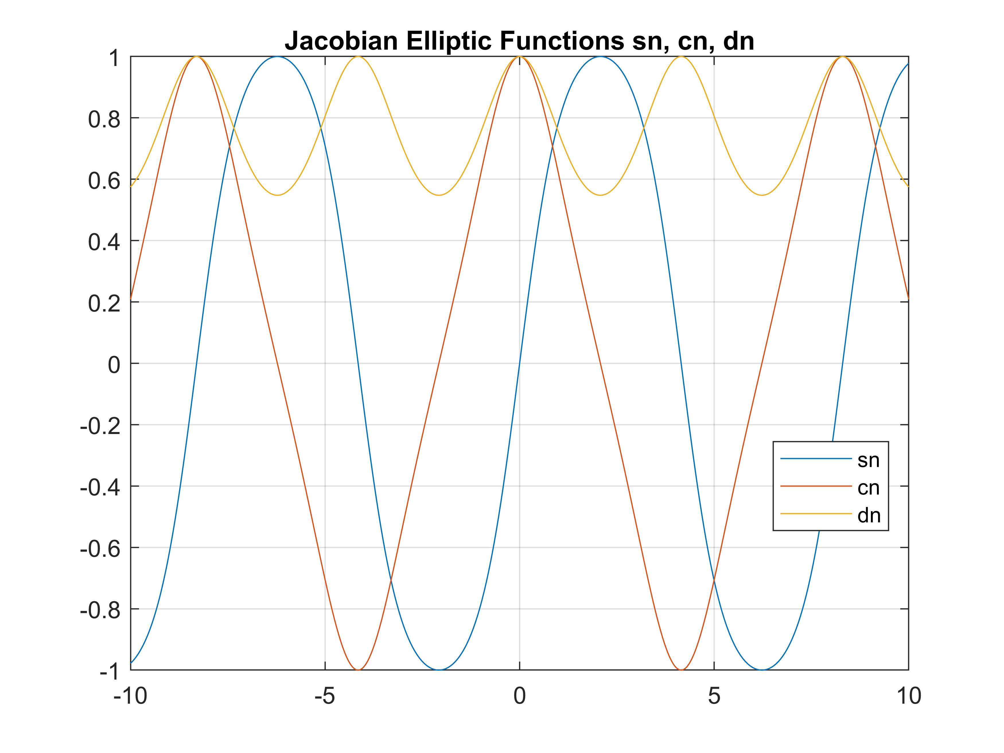
We list all the helpful identities here:
Let :
The addition formulas:
so that
The Jacobian elliptic functions admit an extension to the complex field, which can be computed using the addition formulas on , , .
Proposition 5.
Consider the parametrization of Equation (26), Equation (27) and Equation (28).
- [1]
- [2]
-
[3]
When and :
Hence for the parametrization of Equation (27) when :
The above equation determines in the form of:
When , we need to do the following transformation:
and we could find
Note that when there is a sign change, which is shown in the final expression.
-
[4]
When and :
Hence for the parametrization of Equation (27), when :
The above equation determines in the form of:
When , we need to do the following transformation:
and we could find
Note that when there is a sign change, which is shown in the final expression.
1.
and [2] can be verified by direct calculation. [3] and [4] could be proved by rewritten the addition formulas.
Let , and reform them into polynomials:
Subtract them and divide by we would obtain (3). Further,
Let , and reform them into polynomials:
Subtract them and divide by we would obtain (4). ∎
Similar to the derivation in Conic I, it is still necessary to clarify the magnitudes of .
Proposition 6.
The relation between the magnitudes of and the signs of amplitudes . Note that . .
-
[1]
and imply or :
-
[a]
,
-
[b]
,
-
[a]
-
[2]
and imply or :
-
[a]
,
-
[b]
,
-
[a]
-
[3]
and imply or :
-
[a]
,
-
[b]
,
-
[a]
-
[4]
and imply or :
-
[a]
,
-
[b]
,
-
[a]
Now we are ready to give the solutions for both the real and complexified configuration space.
If :
To calculate with :
| Choice of for real configurations | Branch 1 | Branch 2 |
| , , when , this branch ‘snaps’ at and ‘snaps’ at | , , when , this branch ‘snaps’ at and ‘snaps’ at | |
| , , when , this branch ‘snaps’ at and ‘snaps’ at | , , when , this branch ‘snaps’ at and ‘snaps’ at |
for phase shift:
where
The results in Elliptic I and Elliptic II are formally symmetric, and have a good correspondence with Deltoid II, Conic I, Conic II and Conic III.
23 Orthodiagonal: finite solution
The condition on sector angles is:
and
From the helpful identities listed in Proposition 3, we have the following simplified Equations (6):
That is to say and are separable:
In the parametrized expression, we could obtain , since
and
Further we could say that is half of the quarter period of elliptic functions with modulus :
This is because for half-quarter-periods
If ,
If ,
24 Square: solution at infinity
The condition on sector angles is:
which means:
From post-examination, the solutions at infinity are these two branches of simple folds, each of which is diffeomorphic to a circle .
25 Rhombus: solution at infinity
The condition on sector angles is
which means:
From post-examination, the solutions at infinity are these two branches of simple folds, each of which is diffeomorphic to a circle .
26 Cross: solution at infinity
The condition on sector angles is:
which means:
The solutions at infinity are two isolated points, which are limit points of the finite branches.
27 Miura I: solution at infinity
The condition on sector angles is:
which means:
From post-examination, the solutions at infinity becomes another branch diffeomorphic to a circle :
28 Miura II: solution at infinity
The condition on sector angles is:
which means:
From post-examination, the solutions at infinity becomes another branch diffeomorphic to a circle :
29 Isogram: solution at infinity
The condition on sector angles is
which means:
The solutions at infinity are two isolated points, which are limit points of the finite branches.
30 Anti-isogram: solution at infinity
The condition on sector angles is:
which means:
This is exactly the limit point of the two branches in the finite solution, also called a flat-folded state.
31 Deltoid I: solution at infinity
The condition on sector angles is:
which means:
From post-examination, the solutions at infinity becomes another branch diffeomorphic to a circle :
32 Anti-deltoid I: solution at infinity
The condition on sector angles is:
which means:
For the last two group of points, only one group is real solution, depending on the sign of .
33 Deltoid II: solution at infinity
The condition on sector angles is
which means:
From post-examination, the solutions at infinity becomes another branch diffeomorphic to a circle :
34 Anti-deltoid II: finite solution
The condition on sector angles is
which means:
For the last two group of points, only one group is real solution, depending on the sign of .
35 Conic I: solution at infinity
The condition on sector angles is:
which implies , and:
This is exactly the limit point of the two branches in the finite solution.
36 Conic II: solution at infinity
The condition on sector angles is
From post-examination, the isolated solutions at infinity are:
and when ,
On the other hand, when ,
Note that the two groups of solutions above will switch between real and complex values depending on whether or . Here only real values are admissible solutions at infinity.
37 Conic III: solution at infinity
The condition on sector angles is
From post-examination, the isolated solutions at infinity are:
and, when :
when :
Note that the two groups of solutions above will switch between real and complex value depending on whether or . Here only real values are admissible solutions at infinity.
38 Conic IV: solution at infinity
The condition on sector angles is:
which leads to
From post examination we could obtain the solution similar to Conic II and III.
When ,
When ,
When ,
When ,
Here only two of the four groups are real, while the rest are complex.
39 Elliptic: solution at infinity
The condition on sector angles is:
which leads to
Similarly, our next step is to determine how many of the above solutions are real. Take as an example, the condition for to be real numbers is (referring to the helpful identities in Section 5):
Following the notation introduced for the Elliptic type,
| (29) |
the condition for to be a real configuration is
Let us write all the cases together:
From post-examination, when , reaches the infinity:
When , reaches the infinity:
When , reaches the infinity:
When , reaches the infinity:
40 The Grashof condition and self-intersection
Proposition 7.
(The spherical version of the Grashof condition) If the sum of the shortest and longest linkage of a planar quadrilateral linkage is less than or equal to the sum of the remaining two linkages, then the shortest linkage can rotate fully with respect to a neighbouring linkage.
We could naturally examine this condition from our previous discussions on the solutions at infinity. It holds obviously except for the elliptic type. Without loss of generality, suppose is the shortest linkage, then the condition for or is
Since is the shortest, the statement below holds
hence in order for or can be reached, we need to require:
The right hand side is exactly the Grashof condition.
Proposition 8.
When no folding angle reaches zero or the infinity, a spherical 4-bar linkage is self-intersected if and only if
Proof.
The study of self-intersections of a spherical quadrilateral reduces to study of intersection of two arcs, say, AB and CD. These segments intersect if and only if the points A and B lie on opposite sides of the line CD and the points C and D lie on the opposite sides of the line AB. The points A and B lie on different sides of CD if and only if the oriented areas of the triangles ACD and BCD have different signs. So for a spherical 4-bar linkage ABCD it suffices to compute the oriented areas of all four triangles and to study the pattern of signs. Further, the signs of these oriented areas equal to the signs of the rotational angles . ∎
We have introduced this self-intersection check in the attached MATLAB app.
Acknowledgement
This work is supported by the JST CREST Grant No. JPMJCR1911.
References
- Chen and Chiang (1983) Jen-San Chen and C.H Chiang. Fourth order synthesis of spherical 4-bar function generators. Mechanism and Machine Theory, 18(6):451–456, January 1983. ISSN 0094114X. doi: 10.1016/0094-114X(83)90061-7.
- Foschi et al. (2022) Riccardo Foschi, Thomas C. Hull, and Jason S. Ku. Explicit kinematic equations for degree-4 rigid origami vertices, Euclidean and non-Euclidean. Physical Review E, 106(5):055001, November 2022. doi: 10.1103/PhysRevE.106.055001. Publisher: American Physical Society.
- Gibson and Selig (1988a) C. G. Gibson and J. M. Selig. Movable hinged spherical quadrilaterals – II singularities and reductions. Mechanism and Machine Theory, 23(1):19–24, January 1988a. ISSN 0094-114X. doi: 10.1016/0094-114X(88)90005-5.
- Gibson and Selig (1988b) C.G Gibson and J.M Selig. Movable hinged spherical quadrilaterals – I the configuration space. Mechanism and Machine Theory, 23(1):13–18, January 1988b. ISSN 0094114X. doi: 10.1016/0094-114X(88)90004-3.
- He (2023) Zeyuan He. Elliptic-fun-based config space of spherical 4-bar linkage. MATLAB Central File Exchange, July 2023. https://uk.mathworks.com/matlabcentral/fileexchange/132653-elliptic-fun-based-config-space-of-spherical-4-bar-linkage.
- Izmestiev (2016) Ivan Izmestiev. Classification of flexible Kokotsakis polyhedra with quadrangular base. International Mathematics Research Notices, 2017(3):715–808, 2016. doi: 10.1093/imrn/rnw055.
- Khimshiashvili (2011) G. Khimshiashvili. Complex geometry of quadrilateral linkages. Recent Developments in Generalized Analytic Functions and Their Applications, pages 90–100, 2011.
- Waitukaitis and van Hecke (2016) Scott Waitukaitis and Martin van Hecke. Origami building blocks: Generic and special four-vertices. Physical Review E, 93(2):023003, February 2016. doi: 10.1103/PhysRevE.93.023003. Publisher: American Physical Society.
- Zimmermann and Stanković (2020) Luca Zimmermann and Tino Stanković. Rigid and Flat Foldability of a Degree-Four Vertex in Origami. Journal of Mechanisms and Robotics, 12(1), 2020. Publisher: American Society of Mechanical Engineers Digital Collection.