Minimal model for double Weyl points, multiband quantum geometry,
and singular flat band inspired by LK-99

Moritz M. Hirschmann RIKEN Center for Emergent Matter Science, Wako, Saitama 351-0198, Japan    Johannes Mitscherling Department of Physics, University of California, Berkeley, California 94720, USA
Abstract

Two common difficulties in the design of topological quantum materials are that the desired features lie too far from the Fermi level and are spread over a too large energy range. Doping-induced states at the Fermi level provide a solution, where non-trivial topological properties are enforced by the doping-reduced symmetry. To show this, we consider a regular placement of dopants in a lattice of space group (SG) 176 (P6$\text{}_{3}$/m), which reduces the symmetry to SG 143 (P3). Our two- and four-band models feature symmetry-enforced double Weyl points at $\Gamma$ and A with Chern bands for $k_{z}\neq 0,\pi$, Van Hove singularities, nontrivial multiband quantum geometry due to mixed orbital character, and a singular flat band. The excellent agreement with density-functional theory (DFT) calculations on copper-doped lead apatite (’LK-99’) provides evidence that minimal topological bands at the Fermi level can be realized in doped materials.

Introduction— First experimental and theoretical results on copper-doped lead apatite $\text{Pb}_{10-x}\text{Cu}_{x}(\text{PO}_{4})_{6}\text{O}$ with 0.9$\,<\,$ $x$ $\,<\,$1.1 (’LK-99’) [1, 2, 3, 4, 5, 6, 7, 8, 9, 10, 11, 12, 13] stimulated the question how the doping alters the physical properties of the parent compound. Early density-functional theory (DFT) calculations on $\text{Pb}_{9}\text{Cu}(\text{PO}_{4})_{6}(\text{OH})_{2}$ [5] and $\text{Pb}_{9}\text{Cu}(\text{PO}_{4})_{6}\text{O}$ [6, 7, 8] assumed that a single copper atom replaces one of the four lead atoms on the 4f Wyckoff position. They identified two narrow bands at the Fermi level and two broader bands in the close vicinity. These bands show interesting properties including band crossings at the high-symmetry points $\Gamma$ and A, Van Hove singularities at M and L, and very narrow bands. The character of the relevant bands mainly involve the copper and an extra oxygen from the partially occupied 4e Wyckoff position.

Whereas the DFT studies originally aimed for a better understanding of the experimental results [5, 7, 8, 6], we use their results as an inspiration to tackle common issues in the study of topological band theory [14, 15]. Two difficulties are that (I) the topological features [16, 17, 18] lie too far from the Fermi level and (II) are spread over a too large energy range. Challenge (I) can be addressed by extensive material surveys [19, 20, 21], by pushing interstitial electrons into the gap of a molecular crystal [22], or by defect states within a gap in the vicinity of the Fermi level [23, 24, 25, 26]. Difficulty (II) can be avoided by narrow bands, which are known to occur in hexagonal systems [27, 17, 28]. Our approach expands on the last two ideas.

We construct minimal two- and four-band tight-binding models based on the SG 143 (P3) of the assumed copper-doped crystal structure [5, 6]. Our model exhibits key topological and quantum geometric properties including double Weyl points at $\Gamma$ and A, Chern bands for $k_{z}\neq 0,\pi$, nontrivial Berry curvature and quantum metric for single bands as well as for a combined set of connected bands due to orbital mixing, and a singular flat band resembling the Creutz ladder [29].

Topology via doping-reduced symmetry— As starting point we consider the rich topology of SG 176 ($P6_{3}/m$), the SG of lead apatite [30, 31]. It enforces band crossings on points, lines, and planes [32, 33]. For spinful bands this centrosymmetric group leads to three Dirac nodal lines intersecting at the A point as a result of the off-centered mirror symmetry $m_{z}$ [34]. Systems with spinless representations of $P6_{3}/m$ exhibit always a nodal plane at $k_{z}=\pi$ [35] and Dirac points at $k_{z}=0$ are possible [32].

With doping one site per unit cell one should expect that the space group symmetry is in general reduced. In the absence of a significant structural transition, the new band structure exhibits still the (symmorphic) site symmetry. Specifically, substituting one copper on the 4f Wyckoff position of lead-apatite, as assumed in DFT [5, 7, 8, 6], reduces SG 176 to SG 143 ($P3$) with broken inversion symmetry [36]. Interestingly, the complex spinless representation of $P3$ provides the minimal model for just a pair of Weyl points at the time-reversal invariant momenta (TRIMs) $\Gamma$ and A. In contrast, the spinful representations are known to exhibit eight Kramers-Weyl points [37].

Refer to caption
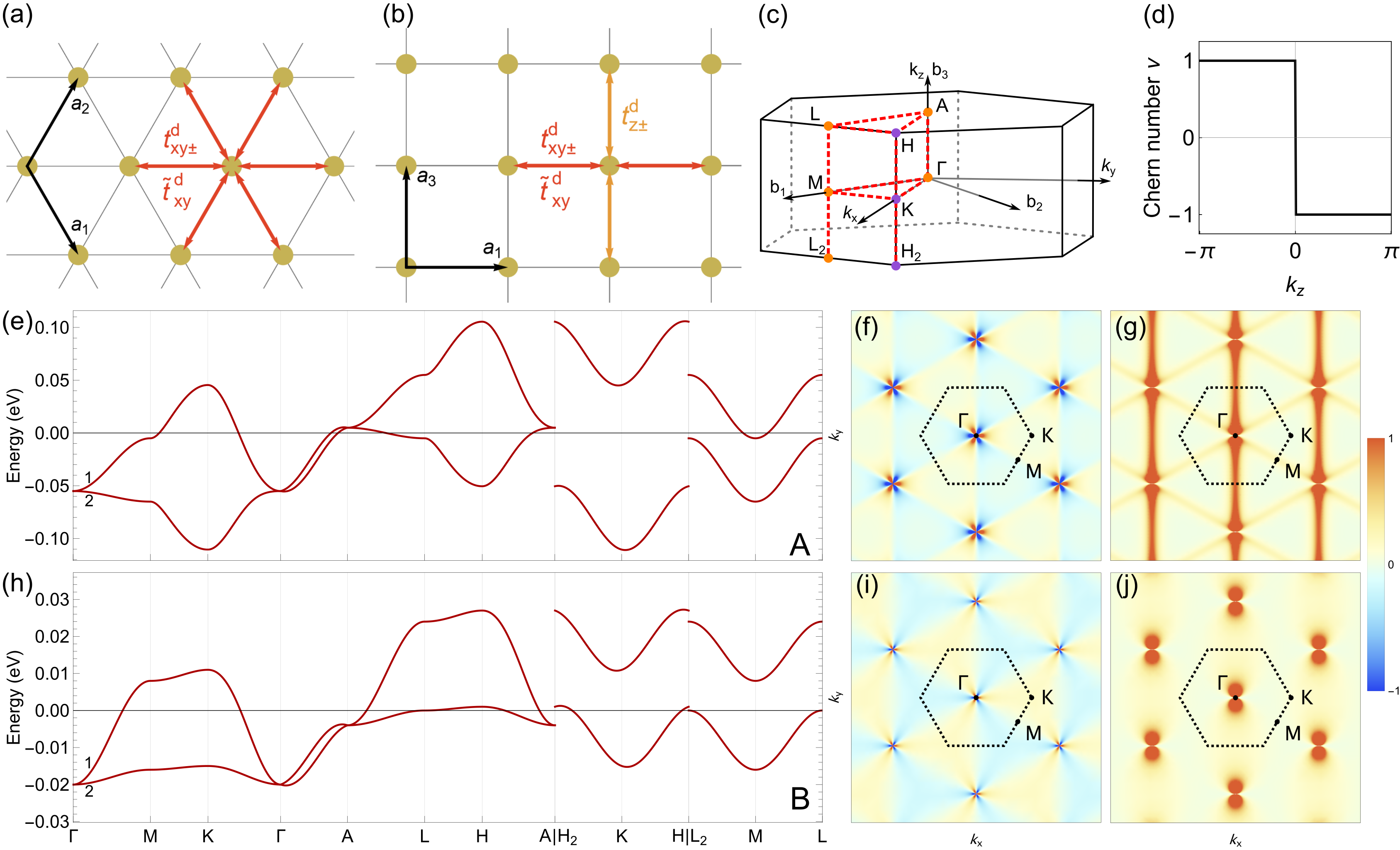
Figure 1: Two-band model for SG P3 (a,b) Top and side view of the trigonal lattice with nearest-neighbor hopping terms, where symmetry-related directions are shown in the same color. 
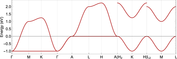
(c) Brillouin zone with TRIMs (orange), high-symmetry points (purple) and k-path (red) that is used for the band structures with parameter sets A and B in (e) and (h), respectively. The parameters are summarized in the supplemental materials (SM) [38]. (d) Symmetry-enforced Chern numbers on planes of constant kzsubscript𝑘𝑧k_{z}. Berry curvature Ω2xysubscriptsuperscriptΩ𝑥𝑦2\Omega^{xy}_{2} (f,i) and quantum metric g2xxsubscriptsuperscript𝑔𝑥𝑥2g^{xx}_{2} (g,h) at kz=0subscript𝑘𝑧0k_{z}=0 corresponding to the models to the left.

Two-band model— To construct an effective model for the doping-induced states in a lattice of SG $P6_{3}/m$, we assume that the relevant states form a lattice with SG $P3$. Without loss of generality, they occupy the 1a Wyckoff position of the trigonal unit cell. We introduce all symmetry-allowed nearest-neighbor hopping terms, see Fig. 1 (a,b). To capture the band topology in a symmetry-enforced fashion, we use the complex representation of the threefold rotation $C_{3}$, created by the operators $\{\hat{d}_{1}^{\dagger},\hat{d}_{2}^{\dagger}\}$ corresponding to the rotation eigenvalues $\mathrm{e}^{2\pi i/3}$ and $\mathrm{e}^{-2\pi i/3}$, respectively. This can capture any band pair comprising $d_{xz}$-, $d_{yz}$-, $d_{x^{2}-y^{2}}$-, and $d_{xy}$-orbital weights [38]. We find the Hamiltonian

$\displaystyle H_{d}(\mathbf{k})$ $\displaystyle=\begin{pmatrix}H_{11}(\mathbf{k})&H_{12}(\mathbf{k})\\[2.84526pt] H^{*}_{12}(\mathbf{k})&H_{22}(\mathbf{k})\end{pmatrix}$ (1)

with

$\displaystyle H_{11}(\mathbf{k})=-\mu_{d}+t^{d}_{z+}\cos\big(\mathbf{k}\cdot\mathbf{a}_{3}\big{missing})+t^{d}_{z-}\,\sin\big(\mathbf{k}\cdot\mathbf{a}_{3}\big{missing})$
$\displaystyle+t^{d}_{xy+}\Big{[}\!\cos\!\big{(}\mathbf{k}\!\cdot\!\mathbf{a}_{1}\big{)}\!+\!\cos\!\big{(}\mathbf{k}\!\cdot\!(\mathbf{a}_{1}\!+\mathbf{a}_{2})\big{)}\!+\cos\!\big{(}\mathbf{k}\!\cdot\!\mathbf{a}_{2}\big{)}\Big{]}$
$\displaystyle+t^{d}_{xy-}\Big{[}\!\sin\!\big{(}\mathbf{k}\!\cdot\!\mathbf{a}_{1}\big{)}-\sin\!\big{(}\mathbf{k}\!\cdot\!(\mathbf{a}_{1}\!+\!\mathbf{a}_{2})\big{)}+\sin\!\big{(}\mathbf{k}\!\cdot\!\mathbf{a}_{2}\big{)}\Big{]}\,,$ (2)
$\displaystyle H_{22}(\mathbf{k})=H_{11}(-\mathbf{k})\,,$ (3)
$\displaystyle H_{12}(\mathbf{k})=\tilde{t}^{d}_{xy}\Big{[}\cos\big(\mathbf{k}\cdot\mathbf{a}_{1}\big{missing})+\mathrm{e}^{i\frac{2\pi}{3}}\cos\big(\mathbf{k}\cdot(\mathbf{a}_{1}+\mathbf{a}_{2})\big{missing})$
$\displaystyle\hskip 71.13188pt+\mathrm{e}^{-i\frac{2\pi}{3}}\cos\big(\mathbf{k}\cdot\mathbf{a}_{2}\big{missing})\Big{]},$ (4)

where we use the lattice vectors $\mathbf{a}_{1}=a(1/2,-\sqrt{3}/2,0)$, $\mathbf{a}_{2}=a(1/2,\sqrt{3}/2,0)$, and $\mathbf{a}_{3}=c(0,0,1)$, setting $a=c=1$. The model has six parameters, the $\mathbf{a}_{1}$-$\mathbf{a}_{2}$-plane hoppings $t^{d}_{xy\pm}$ and $\tilde{t}^{d}_{xy}$, the out-of-plane hoppings $t^{d}_{z\pm}$, and the chemical potential $\mu_{d}$. The subscripts denote the real space directions and whether the hopping is inversion symmetric $(+)$ or antisymmetric $(-)$. We provide longer-range hoppings in the supplemental material (SM) [38]. Two band structures along the path sketched in Fig. 1 (c) are shown in (e) and (h) for different parameter sets [38].

The band gap vanishes at $\Gamma$ and A independent of parameters, as enforced by time-reversal symmetry. The gaps at M and L (K and H) are identical and scale with $|\tilde{t}^{d}_{xy}|$ ($|t^{d}_{xy-}|$). The splitting on $\Gamma$-A is proportional to $|t^{d}_{z-}|$. The comparison of the band curvatures at the band touching points $\Gamma$ and A give insight into the sign of $t^{d}_{xy+}$ and its relative size compared to $|\tilde{t}^{d}_{xy}|$ [38].

Refer to caption
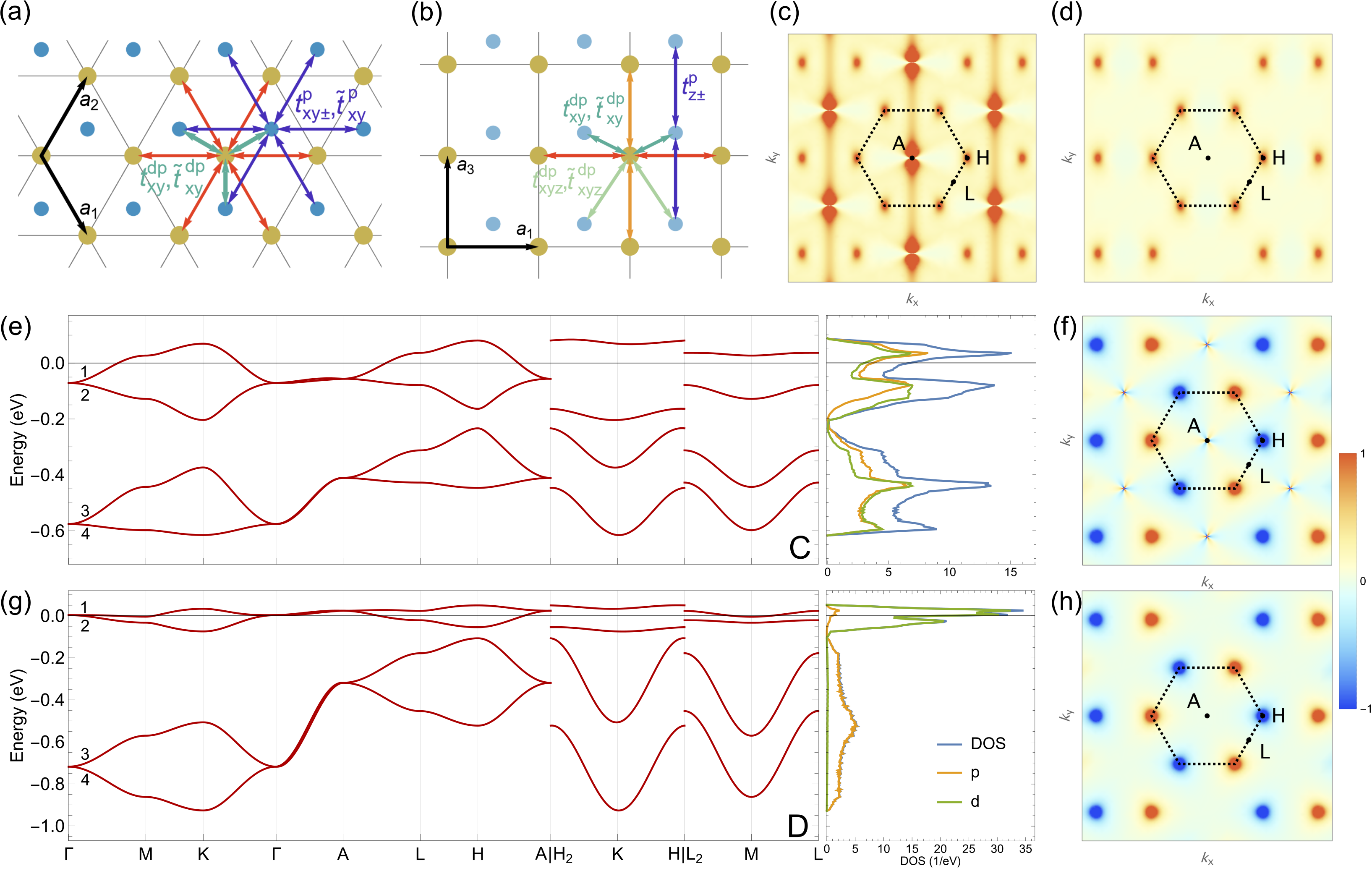
Figure 2: Four-band model for SG P3 (a,b) Top and side view of the trigonal lattice with nearest- and next-nearest-neighbor hopping terms, where symmetry-related directions are shown in the same color. (e,g) Resulting band structures with the corresponding (orbital-resolved) density of states (DOS) for parameter sets C and D [38]. (c,d) Quantum metric $g^{xx}$ for band 2 and bands 1+2 with parameter set C. (f,h) Berry curvature $\Omega^{xy}$ for band 2 and bands 1+2 with parameter set C.

Four-band model— Inspired by the hybridization between the copper Cu and extra-oxygen O or $(\text{OH})_{2}$ orbitals, as seen in DFT [5, 7, 8, 6], we introduce a second site to our lattice on the 1b Wyckoff position of space group $P3$. The resulting second band pair exhibits the complex representation of $P3$, referred to as $\{\hat{p}^{\dagger}_{1},\hat{p}^{\dagger}_{2}\}$. This can capture any band pair comprising $p_{x}$- and $p_{y}$-orbital weights. Our four-band model takes the form

$\displaystyle H_{4\times 4}(\mathbf{k})$ $\displaystyle=\begin{pmatrix}H_{d}(\mathbf{k})&H_{dp}(\mathbf{k})\\[2.84526pt] H^{\dagger}_{dp}(\mathbf{k})&H_{p}(\mathbf{k})\end{pmatrix}\,.$ (5)

The hopping terms, see Fig. 2 (a,b), within each sub-lattice take the same form as in the two-band model. Thus, we keep $H_{d}(\mathbf{k})$ for the $d$ sublattice and define $H_{p}(\mathbf{k})$ for the $p$ sublattice by replacing $d\rightarrow p$ in all indices of $H_{d}(\mathbf{k})$ in Eq. (1). We give the exact form of the inter-sublattice hopping $H_{dp}(\mathbf{k})$ in the SM [38]. Two band structures are shown in Fig. 2 (e) and (g) for different parameter sets [38].

Topology and quantum geometry— Many interesting phenomena are not only related to the energy spectrum but also rely on the wave function properties [39, 40, 41, 42, 43, 44, 45, 46, 47]. Beside the well-known Berry curvature, the quantum metric recently attracted much interest, see e.g. Refs. [48, 49, 50, 51, 52, 53, 54, 55, 56, 57, 58, 59, 60, 61, 62], and has been considered as particularly important in the context of narrow or flat bands [59, 60, 61, 62]. The quantum metric is a measure of the overlap between Bloch states of close-by momenta [63]. We use the convenient mathematical description in terms of gauge-invariant projectors $P_{n}(\mathbf{k})=|u_{n}(\mathbf{k})\rangle\langle u_{n}(\mathbf{k})|$ with eigenstates $|u_{n}(\mathbf{k})\rangle$ of the Hamiltonian [56, 57, 58]. A projector $P_{j}(\mathbf{k})$ on a single band or larger subspace defines the corresponding quantum metric $g^{\alpha\beta}_{j}(\mathbf{k})$ and Berry curvature $\Omega^{\alpha\beta}_{j}(\mathbf{k})$ via

$\displaystyle g^{\alpha\beta}_{j}(\mathbf{k})=\frac{1}{2}\text{Tr}\Big{[}\partial_{\alpha}P_{j}(\mathbf{k})\,\partial_{\beta}P_{j}(\mathbf{k})\Big{]}\,,$ (6)
$\displaystyle\Omega^{\alpha\beta}_{j}(\mathbf{k})=\text{Tr}\Big{[}P_{j}(\mathbf{k})\partial_{\alpha}P_{j}(\mathbf{k})\partial_{\beta}P_{j}(\mathbf{k})\Big{]}-(\alpha\leftrightarrow\beta)\,,$ (7)

with trace Tr and momentum derivative $\partial_{\alpha}=\partial_{k_{\alpha}}$ in direction $\alpha$. Note that the quantum metric is in general non-additive, that is $g^{\alpha\beta}_{(12)}=g^{\alpha\beta}_{1}+g^{\alpha\beta}_{2}+\text{Tr}\big{[}\partial_{\alpha}P_{1}\partial_{\beta}P_{2}\big{]}$ when $P_{(12)}=P_{1}+P_{2}$, where the last cross-term involves the projector of both bands 1 and 2 [57]. The general theory of quantum geometry beyond single particle projectors has recently received increasing interest [58, 64].

As expected for spinless representations [65, 66], we find double Weyl points with Chern number $\nu=-2$ and $\nu=+2$ at $\Gamma$ and A, respectively, as shown in Fig. 1 (d) [67]. We show the Berry curvature $\Omega^{xy}_{2}$ in Fig. 1 (f,i) and the quantum metric $g^{xx}_{2}$ in (g,j) for $k_{z}=0$, where the Weyl points lead to divergences. Depending on the gap size on $\Gamma$-A [38], the Berry curvature in Fig. 1 (f) is larger compared to (i). Whereas the quantum metric is only large around $\Gamma$ in Fig. 1 (j), it has extended regions with larger contributions in (g). More than two bands are required to see nontrivial effects of multiband geometry since the geometry of the combined bands vanishes for a two-band model, $g^{xx}_{(12)}=\Omega^{xy}_{(12)}=0$.

In Fig. 2 (c,d,f,h), we show the Berry curvature $\Omega^{xy}$ and quantum metric $g^{xx}$ at $k_{z}=\pi$ for the four-band model C [38] with band structure and density of state shown in (e). Here, both $d$ and $p$ sites have the same chemical potential $\mu_{d}=\mu_{p}$, which requires a strong d-p coupling $H_{dp}$ in order to obtain the shown band gap. This implies a large orbital mixing between bands. Indeed, the quantum metric $g^{xx}_{2}$ of band 2 shows additional features at H, see (c), which are not present in the two-band model. As shown in (d), these features are present in the quantum metric $g^{xx}_{(12)}$ of the combined bands 1 and 2. This metric shows no singularity, as expected, because the singularities are compensated by the additional cross-term [57]. In (f) and (h) we show the Berry curvature $\Omega^{xy}_{2}$ and $\Omega^{xy}_{(12)}$, respectively. Similarly to the quantum metric, we observe no divergence and find additional contributions at H due to the band gap minimum between band 2 and 3. The four-band model D [38] has only weak d-p coupling and does not show significant additional features compared to the two-band model.

The quantum geometry of an isolated subspace of bands is an interesting property connected to new geometric effects in narrow or flat bands, where the interaction strength exceeds the subspace band width [48, 68, 62, 69]. A key quantity is the integrated quantum metric $\bar{g}_{(12)}\equiv\int\frac{d^{3}\mathbf{k}}{V}\tr g_{(12)}(\mathbf{k})$ with $V=16\pi^{3}/\sqrt{3}$, which can be interpreted as the gauge-invariant part of the Wannier function variance [70]. We find $\bar{g}_{(12)}=0.26$ and $\bar{g}_{(12)}=0.03$ for model C and D, respectively. Geometric contributions to observables are, thus, expected to be significantly larger for model C than D.

Singular flat band— Flat bands have attracted huge interest in the last years, see for instance Refs. [71, 72, 73, 74, 75]. A particular class of flat bands has its origin in destructive interference during the hopping process, so-called frustrated lattices, and has been widely discussed in the literature [76, 77, 78, 79, 80, 81, 82, 83, 84, 85]. It is quite intuitive that such an effect could also lead to a flat band in this case due to the combination of a triangular lattice structure and an orbital degree of freedom.

Indeed, our two-band model exhibits a flat band at kz=0,πsubscript𝑘𝑧0𝜋k_{z}=0,\pi for 2txy+d=±|t~xyd|2subscriptsuperscript𝑡𝑑limit-from𝑥𝑦plus-or-minussubscriptsuperscript~𝑡𝑑𝑥𝑦2t^{d}_{xy+}=\pm|\tilde{t}^{d}_{xy}| and 2txyd=±3|t~xyd|2subscriptsuperscript𝑡𝑑limit-from𝑥𝑦plus-or-minus3subscriptsuperscript~𝑡𝑑𝑥𝑦2t^{d}_{xy-}=\pm\sqrt{3}|\tilde{t}^{d}_{xy}|. The band remains flat for all kzsubscript𝑘𝑧k_{z} if tzd=0subscriptsuperscript𝑡𝑑limit-from𝑧0t^{d}_{z-}=0. If tzd0subscriptsuperscript𝑡𝑑limit-from𝑧0t^{d}_{z-}\neq 0 the flat band gets dispersive for kz0subscript𝑘𝑧0k_{z}\neq 0 as expected due to the finite Chern number. Thus, we can identify it as a singular flat band [86, 38]. 
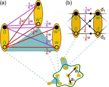
A nonorthogonal compact localized eigenstate involves a site and its six nearest neighbors in the x𝑥x-y𝑦y plane, see Fig. 3. The weights are such that they destructively interfere with each other under intra- and inter-orbital hopping, which resembles the Creutz ladder known in 1d [29, 87, 88, 89].

Refer to caption
Figure 3: Visualization of the compact localized state of the singular flat band and the destructive interference for triangles (a) and lines (b). The orbital weights (green) and hoppings (red, purple) involve $w=(1+i\sqrt{3})/2$, see SM for further details [38].

Application to LK-99— Our band structures shown in Fig. 1 (e,h) and 2 (e,g) are able to reproduce most of the key features reported in the early DFT studies on copper-doped lead apatite [5, 7, 8, 6]. For the two-band model we have identified two parameter sets A and B [38] to capture the band structure differences connected to the relative position of copper and extra oxygen sites [8]. Parameter set B generates the reported almost flat band [5, 8], see also the phenomenological flat-band model in Ref. [12]. Our model shows saddle-point Van Hove singularities in all bands at M and L with an energy profile as reported in Ref. [8]. Via our analysis we identify the reported band crossings at $\Gamma$ and A as double Weyl points. A finite value of $t^{d}_{z-}$ captures the small splitting of the otherwise degenerate bands along the $\Gamma$-A line.

The same aspects are also reproduced in the four-band model with parameter sets C and D [38]. C is constructed to reproduce the nearly equal distribution of p and d orbitals in the density of states, shown in Fig. 2 (e), which was seen in the DFT results [5, 7, 8, 6] for bands 1 and 2. The weak d character of bands 3 and 4 in the DFT results cannot be captured by just four bands. Model D corresponds to a weakly coupled four-band model with mixing of d and p orbitals of at most 10%.

Further theoretical and experimental studies on LK-99 were published very recently [90, 91, 92, 93, 94, 95, 96, 97, 98, 99, 100, 101, 102, 103, 104]. In several DFT studies, tight-binding models were constructed [101, 91, 92, 93, 94, 95, 96, 97] and their parameters are reasonably close to ours. Note that these models use cubic harmonics, whereas our models correspond to $C_{3}$-symmetric combinations of d and p orbitals [38]. P. Lee and Z. Dai [90] study the low-energy physics of LK-99, arguing that it may be in proximity to the metal insulator transition at integer filling. Their argument is based on the ratio between the potential difference of the Cu and O sites and the hopping between them. They estimated similar parameters as in our model D. The topology and quantum geometry analyzed in Ref. [101] align with our conclusions. The symmetry group of doped and undoped lead apatite was revisited [98, 99] and the importance of lattice distortions was highlighted [100]. The originally proposed unusual resistivity signatures in LK-99 [1, 2] were connected to a $\text{CuS}_{2}$ impurity phase by recent experimental studies [101, 102, 103, 104].

Conclusion— We present doping-induced states at the Fermi level as a tool to design systems with topological and geometrical band structures via doping-reduced symmetries. Analogously to the presented example, our method can be applied to other dopant configurations as well as other insulating materials doped with transition metal ions [100]. The corresponding tight-binding models enable the study of disorder, interaction, material realization [105, 106, 107, 108, 109, 82], narrow and flat-band systems [110, 111, 112] and their unique physics [113, 114, 48, 115, 116, 69, 68, 117, 118, 119, 120, 28, 121, 122, 123].

Acknowledgements.
The authors thank Alexander Avdoshkin, Zhehao Dai, Tomohiro Soejima, Jan M. Tomczak, and Taige Wang for very stimulating discussions. M. M. H. is funded by the Deutsche Forschungsgemeinschaft (DFG, German Research Foundation) - project number 518238332. J. M. acknowledges support by the German National Academy of Sciences Leopoldina through Grant No. LPDS 2022-06.

M. M. H. and J. M. contributed equally to this work.

References

  • Lee et al. [2023a] S. Lee, J.-H. Kim, and Y.-W. Kwon, The first room-temperature ambient-pressure superconductor (2023a), arXiv:2307.12008 [cond-mat.supr-con] .
  • Lee et al. [2023b] S. Lee, J. Kim, H.-T. Kim, S. Im, S. An, and K. H. Auh, Superconductor $\text{Pb}_{10-x}\text{Cu}_{x}(\text{PO}_{4})_{6}\text{O}$ showing levitation at room temperature and atmospheric pressure and mechanism (2023b), arXiv:2307.12037 [cond-mat.supr-con] .
  • Hou et al. [2023] Q. Hou, W. Wei, X. Zhou, Y. Sun, and Z. Shi, Observation of zero resistance above $100^{\circ}\,\text{K}$ in $\text{Pb}_{10-x}\text{Cu}_{x}(\text{PO}_{4})_{6}\text{O}$ (2023), arXiv:2308.01192 [cond-mat.supr-con] .
  • Kumar et al. [2023] K. Kumar, N. K. Karn, and V. P. S. Awana, Synthesis of possible room temperature superconductor $\text{LK-}99$: $\text{Pb}_{9}\text{Cu}(\text{PO}_{4})_{6}\text{O}$ (2023), arXiv:2307.16402 [cond-mat.supr-con] .
  • Griffin [2023] S. M. Griffin, Origin of correlated isolated flat bands in copper-substituted lead phosphate apatite (2023), arXiv:2307.16892 [cond-mat.supr-con] .
  • Kurleto et al. [2023] R. Kurleto, S. Lany, D. Pashov, S. Acharya, M. van Schilfgaarde, and D. S. Dessau, Pb-apatite framework as a generator of novel flat-band cuo based physics, including possible room temperature superconductivity (2023), arXiv:2308.00698 [cond-mat.supr-con] .
  • Si and Held [2023] L. Si and K. Held, Electronic structure of the putative room-temperature superconductor $\text{Pb}_{9}\text{Cu}(\text{PO}_{4})_{6}\text{O}$ (2023), arXiv:2308.00676 [cond-mat.supr-con] .
  • Lai et al. [2023] J. Lai, J. Li, P. Liu, Y. Sun, and X.-Q. Chen, First-principles study on the electronic structure of $\text{Pb}_{10-x}\text{Cu}_{x}(\text{PO}_{4})_{6}\text{O}$ $(x=0,1)$ (2023), arXiv:2307.16040 [cond-mat.mtrl-sci] .
  • Abramian et al. [2023] P. Abramian, A. Kuzanyan, V. Nikoghosyan, S. Teknowijoyo, and A. Gulian, Some remarks on possible superconductivity of composition $\text{Pb}_{9}\text{CuP}_{6}\text{O}_{25}$ (2023), arXiv:2308.01723 [cond-mat.supr-con] .
  • Liu et al. [2023] L. Liu, Z. Meng, X. Wang, H. Chen, Z. Duan, X. Zhou, H. Yan, P. Qin, and Z. Liu, Semiconducting transport in $\text{Pb}_{10-x}\text{Cu}_{x}(\text{PO}_{4})_{6}\text{O}$ sintered from $\text{Pb}_{2}\text{SO}_{5}$ and $\text{Cu}_{3}p$ (2023), arXiv:2307.16802 [cond-mat.supr-con] .
  • Baskaran [2023] G. Baskaran, Broad band mott localization is all you need for hot superconductivity: Atom mott insulator theory for $\text{Cu}-\text{Pb}$ apatite (2023), arXiv:2308.01307 [cond-mat.supr-con] .
  • Tavakol and Scaffidi [2023] O. Tavakol and T. Scaffidi, Minimal model for the flat bands in copper-substituted lead phosphate apatite (2023), arXiv:2308.01315 [cond-mat.supr-con] .
  • Oh and Zhang [2023] H. Oh and Y.-H. Zhang, S-wave pairing in a two-orbital t-j model on triangular lattice: possible application to $\text{Pb}_{10-x}\text{Cu}_{x}(\text{PO}_{4})_{6}\text{O}$ (2023), arXiv:2308.02469 [cond-mat.supr-con] .
  • Hasan and Kane [2010] M. Z. Hasan and C. L. Kane, Colloquium: topological insulators, Reviews of modern physics 82, 3045 (2010).
  • Chiu et al. [2016] C.-K. Chiu, J. C. Y. Teo, A. P. Schnyder, and S. Ryu, Classification of topological quantum matter with symmetries, Rev. Mod. Phys. 88, 035005 (2016).
  • Burkov [2016] A. Burkov, Topological semimetals, Nature materials 15, 1145 (2016).
  • Chan et al. [2016] Y.-H. Chan, C.-K. Chiu, M. Y. Chou, and A. P. Schnyder, $\text{Ca}_{3}\text{P}_{2}$ and other topological semimetals with line nodes and drumhead surface states, Phys. Rev. B 93, 205132 (2016).
  • Bernevig et al. [2018] A. Bernevig, H. Weng, Z. Fang, and X. Dai, Recent progress in the study of topological semimetals, Journal of the Physical Society of Japan 87, 041001 (2018).
  • Vergniory et al. [2019] M. Vergniory, L. Elcoro, C. Felser, N. Regnault, B. A. Bernevig, and Z. Wang, A complete catalogue of high-quality topological materials, Nature 566, 480 (2019).
  • Choudhary et al. [2019] K. Choudhary, K. F. Garrity, and F. Tavazza, High-throughput discovery of topologically non-trivial materials using spin-orbit spillage, Scientific reports 9, 8534 (2019).
  • Xu et al. [2020] Y. Xu, L. Elcoro, Z.-D. Song, B. J. Wieder, M. Vergniory, N. Regnault, Y. Chen, C. Felser, and B. A. Bernevig, High-throughput calculations of magnetic topological materials, Nature 586, 702 (2020).
  • Yu et al. [2023] T. Yu, R. Arita, and M. Hirayama, Interstitial-electron-induced topological molecular crystals, Advanced Physics Research 2, 2200041 (2023).
  • Noh et al. [2014] J.-Y. Noh, H. Kim, and Y.-S. Kim, Stability and electronic structures of native defects in single-layer ${\mathrm{mos}}_{2}$Phys. Rev. B 89, 205417 (2014).
  • Trainer et al. [2022] D. J. Trainer, J. Nieminen, F. Bobba, B. Wang, X. Xi, A. Bansil, and M. Iavarone, Visualization of defect induced in-gap states in monolayer mos2, npj 2D Materials and Applications 6, 13 (2022).
  • Schultz [2006] P. A. Schultz, Theory of defect levels and the “band gap problem” in silicon, Phys. Rev. Lett. 96, 246401 (2006).
  • Kim et al. [2023] H. Kim, C.-g. Oh, and J.-W. Rhim, General construction scheme for geometrically nontrivial flat band models (2023), arXiv:2305.00448 [cond-mat.str-el] .
  • Nishino et al. [2003] S. Nishino, M. Goda, and K. Kusakabe, Flat bands of a tight-binding electronic system with hexagonal structure, Journal of the Physical Society of Japan 72, 2015 (2003).
  • Liu et al. [2020] Z. Liu, M. Li, Q. Wang, G. Wang, C. Wen, K. Jiang, X. Lu, S. Yan, Y. Huang, D. Shen, et al., Orbital-selective dirac fermions and extremely flat bands in frustrated kagome-lattice metal CoSn, Nature communications 11, 4002 (2020).
  • Creutz [1999] M. Creutz, End states, ladder compounds, and domain-wall fermions, Phys. Rev. Lett. 83, 2636 (1999).
  • Brückner et al. [1995] S. Brückner, G. Lusvardi, L. Menabue, and M. Saladini, Crystal structure of lead hydroxyapatite from powder x-ray diffraction data, Inorganica Chimica Acta 236, 209 (1995).
  • Krivovichev and Burns [2003] S. V. Krivovichev and P. C. Burns, Crystal chemistry of lead oxide phosphates: crystal structures of $\text{Pb}_{4}\text{O}(\text{PO}_{4})_{2}$, $\text{Pb}_{8}\text{O}_{5}(\text{PO}_{4})_{2}$ and $\text{Pb}_{1}0(\text{PO}_{4})_{6}\text{O}$, Zeitschrift für Kristallographie-Crystalline Materials 218, 357 (2003).
  • Bradlyn et al. [2017] B. Bradlyn, L. Elcoro, J. Cano, M. G. Vergniory, Z. Wang, C. Felser, M. I. Aroyo, and B. A. Bernevig, Topological quantum chemistry, Nature 547, 298 (2017).
  • Zhang et al. [2018] J. Zhang, Y.-H. Chan, C.-K. Chiu, M. G. Vergniory, L. M. Schoop, and A. P. Schnyder, Topological band crossings in hexagonal materials, Physical Review Materials 2, 074201 (2018).
  • Yang et al. [2017] B.-J. Yang, T. A. Bojesen, T. Morimoto, and A. Furusaki, Topological semimetals protected by off-centered symmetries in nonsymmorphic crystals, Physical Review B 95, 075135 (2017).
  • Wilde et al. [2021] M. A. Wilde, M. Dodenhöft, A. Niedermayr, A. Bauer, M. M. Hirschmann, K. Alpin, A. P. Schnyder, and C. Pfleiderer, Symmetry-enforced topological nodal planes at the fermi surface of a chiral magnet, Nature 594, 374 (2021).
  • Tokura and Nagaosa [2018] Y. Tokura and N. Nagaosa, Nonreciprocal responses from non-centrosymmetric quantum materials, Nature communications 9, 3740 (2018).
  • Chang et al. [2018] G. Chang, B. J. Wieder, F. Schindler, D. S. Sanchez, I. Belopolski, S.-M. Huang, B. Singh, D. Wu, T.-R. Chang, T. Neupert, et al., Topological quantum properties of chiral crystals, Nature materials 17, 978 (2018).
  • [38] In this Supplemental Material (SM), we give (i) the used parameters for our two- and four-band model and provide further details of (ii) the constructed two-band model, (iii) the constructed four-band model, and (iv) the analysis of the flat-band including a concrete example.
  • Resta [1994] R. Resta, Macroscopic polarization in crystalline dielectrics: The geometric phase approach, Reviews of Modern Physics 66, 899 (1994).
  • Souza and Vanderbilt [2008] I. Souza and D. Vanderbilt, Dichroic f -sum rule and the orbital magnetization of crystals, Physical Review B 77, 054438 (2008).
  • Souza et al. [2000] I. Souza, T. Wilkens, and R. M. Martin, Polarization and localization in insulators: Generating function approach, Physical Review B 62, 1666 (2000).
  • Resta [2011] R. Resta, The insulating state of matter: A geometrical theory, The European Physical Journal B 79, 121 (2011).
  • Nagaosa et al. [2010] N. Nagaosa, J. Sinova, S. Onoda, A. H. MacDonald, and N. P. Ong, Anomalous hall effect, Rev. Mod. Phys. 82, 1539 (2010).
  • Raoux et al. [2015] A. Raoux, F. Piéchon, J.-N. Fuchs, and G. Montambaux, Orbital magnetism in coupled-bands models, Phys. Rev. B 91, 085120 (2015).
  • Nagaosa et al. [2020] N. Nagaosa, T. Morimoto, and Y. Tokura, Transport, magnetic and optical properties of Weyl materials, Nature Reviews Materials 10.1038/s41578-020-0208-y (2020).
  • Orenstein et al. [2021] J. Orenstein, J. Moore, T. Morimoto, D. Torchinsky, J. Harter, and D. Hsieh, Topology and Symmetry of Quantum Materials via Nonlinear Optical Responses, Annual Review of Condensed Matter Physics 12, 247 (2021).
  • Ma et al. [2021] Q. Ma, A. G. Grushin, and K. S. Burch, Topology and geometry under the nonlinear electromagnetic spotlight, Nature Materials 10.1038/s41563-021-00992-7 (2021).
  • Peotta and Törmä [2015] S. Peotta and P. Törmä, Superfluidity in topologically nontrivial flat bands, Nature Communications 6, 8944 (2015).
  • Holder et al. [2020] T. Holder, D. Kaplan, and B. Yan, Consequences of time-reversal-symmetry breaking in the light-matter interaction: Berry curvature, quantum metric, and diabatic motion, Phys. Rev. Res. 2, 033100 (2020).
  • Mitscherling [2020] J. Mitscherling, Longitudinal and anomalous hall conductivity of a general two-band model, Phys. Rev. B 102, 165151 (2020).
  • Komissarov et al. [2023] I. Komissarov, T. Holder, and R. Queiroz, The quantum geometric origin of capacitance in insulators (2023), arXiv:2306.08035 [cond-mat.mes-hall] .
  • Morimoto et al. [2023] T. Morimoto, S. Kitamura, and N. Nagaosa, Geometric aspects of nonlinear and nonequilibrium phenomena, Journal of the Physical Society of Japan 92, 072001 (2023)https://doi.org/10.7566/JPSJ.92.072001 .
  • Ahn et al. [2020] J. Ahn, G.-Y. Guo, and N. Nagaosa, Low-frequency divergence and quantum geometry of the bulk photovoltaic effect in topological semimetals, Phys. Rev. X 10, 041041 (2020).
  • Ahn et al. [2022] J. Ahn, G.-Y. Guo, N. Nagaosa, and A. Vishwanath, Riemannian geometry of resonant optical responses, Nature Physics 18, 290 (2022).
  • Tai and Claassen [2023] W. T. Tai and M. Claassen, Quantum-geometric light-matter coupling in correlated quantum materials (2023), arXiv:2303.01597 [cond-mat.str-el] .
  • Graf and Piéchon [2021] A. Graf and F. Piéchon, Berry curvature and quantum metric in $n$-band systems: An eigenprojector approach, Phys. Rev. B 104, 085114 (2021).
  • Mera and Mitscherling [2022] B. Mera and J. Mitscherling, Nontrivial quantum geometry of degenerate flat bands, Phys. Rev. B 106, 165133 (2022).
  • Avdoshkin and Popov [2023] A. Avdoshkin and F. K. Popov, Extrinsic geometry of quantum states, Physical Review B 10710.1103/physrevb.107.245136 (2023).
  • Herzog-Arbeitman et al. [2022a] J. Herzog-Arbeitman, A. Chew, K.-E. Huhtinen, P. Törmä, and B. A. Bernevig, Many-body superconductivity in topological flat bands (2022a), arXiv:2209.00007 [cond-mat.str-el] .
  • Herzog-Arbeitman et al. [2022b] J. Herzog-Arbeitman, V. Peri, F. Schindler, S. D. Huber, and B. A. Bernevig, Superfluid weight bounds from symmetry and quantum geometry in flat bands, Phys. Rev. Lett. 128, 087002 (2022b).
  • Bouzerar and Mayou [2021] G. Bouzerar and D. Mayou, Quantum transport in flat bands and supermetallicity, Phys. Rev. B 103, 075415 (2021).
  • Mitscherling and Holder [2022] J. Mitscherling and T. Holder, Bound on resistivity in flat-band materials due to the quantum metric, Phys. Rev. B 105, 085154 (2022).
  • Provost and Vallee [1980] J. P. Provost and G. Vallee, Riemannian Structure on Manifolds of Quantum States, Communications in Mathematical Physics 76, 289 (1980).
  • Bouhon et al. [2023] A. Bouhon, A. Timmel, and R.-J. Slager, Quantum geometry beyond projective single bands (2023), arXiv:2303.02180 [cond-mat.mes-hall] .
  • Tsirkin et al. [2017] S. S. Tsirkin, I. Souza, and D. Vanderbilt, Composite weyl nodes stabilized by screw symmetry with and without time-reversal invariance, Physical Review B 96, 045102 (2017).
  • Alpin et al. [2023] K. Alpin, M. M. Hirschmann, N. Heinsdorf, A. Leonhardt, W. Y. Yau, X. Wu, and A. P. Schnyder, Fundamental laws of chiral band crossings: local constraints, global constraints, and topological phase diagrams, arXiv preprint arXiv:2303.01477  (2023).
  • Fukui et al. [2005] T. Fukui, Y. Hatsugai, and H. Suzuki, Chern numbers in discretized brillouin zone: efficient method of computing (spin) hall conductances, Journal of the Physical Society of Japan 74, 1674 (2005).
  • Hofmann et al. [2020] J. S. Hofmann, E. Berg, and D. Chowdhury, Superconductivity, pseudogap, and phase separation in topological flat bands, Phys. Rev. B 102, 201112 (2020).
  • Mao and Chowdhury [2023] D. Mao and D. Chowdhury, Diamagnetic response and phase stiffness for interacting isolated narrow bands, Proceedings of the National Academy of Sciences 120, e2217816120 (2023).
  • Marzari et al. [2012] N. Marzari, A. A. Mostofi, J. R. Yates, I. Souza, and D. Vanderbilt, Maximally localized wannier functions: Theory and applications, Rev. Mod. Phys. 84, 1419 (2012).
  • Bistritzer and MacDonald [2011] R. Bistritzer and A. H. MacDonald, Moire bands in twisted double-layer graphene, Proceedings of the National Academy of Sciences 108, 12233 (2011).
  • Cao et al. [2018a] Y. Cao, V. Fatemi, A. Demir, S. Fang, S. L. Tomarken, J. Y. Luo, J. D. Sanchez-Yamagishi, K. Watanabe, T. Taniguchi, E. Kaxiras, R. C. Ashoori, and P. Jarillo-Herrero, Correlated insulator behaviour at half-filling in magic-angle graphene superlattices, Nature 556, 80 (2018a).
  • Cao et al. [2018b] Y. Cao, V. Fatemi, S. Fang, K. Watanabe, T. Taniguchi, E. Kaxiras, and P. Jarillo-Herrero, Unconventional superconductivity in magic-angle graphene superlattices, Nature 556, 43 (2018b).
  • Phong and Mele [2023] V. o. T. Phong and E. J. Mele, Quantum geometric oscillations in two-dimensional flat-band solids, Phys. Rev. Lett. 130, 266601 (2023).
  • Sun et al. [2011] K. Sun, Z. Gu, H. Katsura, and S. Das Sarma, Nearly flatbands with nontrivial topology, Phys. Rev. Lett. 106, 236803 (2011).
  • Derzhko et al. [2015] O. Derzhko, J. Richter, and M. Maksymenko, Strongly correlated flat-band systems: The route from Heisenberg spins to Hubbard electrons, International Journal of Modern Physics B 29, 1530007 (2015).
  • Mielke [1991a] A. Mielke, Ferromagnetic ground states for the Hubbard model on line graphs, Journal of Physics A: Mathematical and General 24, L73 (1991a).
  • Mielke [1991b] A. Mielke, Ferromagnetism in the Hubbard model on line graphs and further considerations, Journal of Physics A: Mathematical and General 24, 3311 (1991b).
  • Tasaki [1998] H. Tasaki, From Nagaoka’s Ferromagnetism to Flat-Band Ferromagnetism and Beyond: An Introduction to Ferromagnetism in the Hubbard Model, Progress of Theoretical Physics 99, 489 (1998)https://academic.oup.com/ptp/article-pdf/99/4/489/5209512/99-4-489.pdf .
  • Bergman et al. [2008] D. L. Bergman, C. Wu, and L. Balents, Band touching from real-space topology in frustrated hopping models, Phys. Rev. B 78, 125104 (2008).
  • Pyykkönen et al. [2021] V. A. J. Pyykkönen, S. Peotta, P. Fabritius, J. Mohan, T. Esslinger, and P. Törmä, Flat-band transport and josephson effect through a finite-size sawtooth lattice, Phys. Rev. B 103, 144519 (2021).
  • Kim and Liu [2023] D. Kim and F. Liu, Realization of flat bands by lattice intercalation in kagome metals, Phys. Rev. B 107, 205130 (2023).
  • Kobayashi et al. [2016] K. Kobayashi, M. Okumura, S. Yamada, M. Machida, and H. Aoki, Superconductivity in repulsively interacting fermions on a diamond chain: Flat-band-induced pairing, Phys. Rev. B 94, 214501 (2016).
  • Maimaiti et al. [2017] W. Maimaiti, A. Andreanov, H. C. Park, O. Gendelman, and S. Flach, Compact localized states and flat-band generators in one dimension, Phys. Rev. B 95, 115135 (2017).
  • Häusler [2015] W. Häusler, Flat-band conductivity properties at long-range coulomb interactions, Phys. Rev. B 91, 041102 (2015).
  • Rhim and Yang [2019] J.-W. Rhim and B.-J. Yang, Classification of flat bands according to the band-crossing singularity of bloch wave functions, Phys. Rev. B 99, 045107 (2019).
  • Müller et al. [2016] P. Müller, J. Richter, and O. Derzhko, Hubbard models with nearly flat bands: Ground-state ferromagnetism driven by kinetic energy, Phys. Rev. B 93, 144418 (2016).
  • Mondaini et al. [2018] R. Mondaini, G. G. Batrouni, and B. Grémaud, Pairing and superconductivity in the flat band: Creutz lattice, Phys. Rev. B 98, 155142 (2018).
  • Mahyaeh et al. [2022] I. Mahyaeh, T. Köhler, A. M. Black-Schaffer, and A. Kantian, Superconducting pairing from repulsive interactions of fermions in a flat-band system, Phys. Rev. B 106, 125155 (2022).
  • Lee and Dai [2023] P. A. Lee and Z. Dai, Effective model for $\text{Pb}_{9}\text{Cu}(\text{PO}_{4})_{6}\text{O}$ (2023), arXiv:2308.04480 [cond-mat.supr-con] .
  • Fidrysiak et al. [2023] M. Fidrysiak, A. P. Kadzielawa, and J. Spalek, High temperature superconductivity with strong correlations and disorder: Possible relevance to cu-doped apatite (2023), arXiv:2308.03948 [cond-mat.supr-con] .
  • Si et al. [2023] L. Si, M. Wallerberger, A. Smolyanyuk, S. di Cataldo, J. M. Tomczak, and K. Held, $\text{Pb}_{10-x}\text{Cu}_{x}(\text{PO}_{4})_{6}\text{O}$: a mott or charge transfer insulator in need of further doping for (super)conductivity (2023), arXiv:2308.04427 [cond-mat.supr-con] .
  • Mao et al. [2023] N. Mao, N. Peshcherenko, and Y. Zhang, Wannier functions, minimal model and charge transfer in $\text{Pb}_{9}\text{CuP}_{6}\text{O}_{25}$ (2023), arXiv:2308.05528 [cond-mat.supr-con] .
  • Yue et al. [2023] C. Yue, V. Christiansson, and P. Werner, Correlated electronic structure of $\text{Pb}_{10-x}\text{Cu}_{x}(\text{PO}_{4})_{6}\text{O}$ (2023), arXiv:2308.04976 [cond-mat.str-el] .
  • Bai et al. [2023] H. Bai, L. Gao, and C. Zeng, Ferromagnetic ground state and spin-orbit coupling induced bandgap open in LK99 (2023), arXiv:2308.05134 [cond-mat.supr-con] .
  • Korotin et al. [2023] D. M. Korotin, D. Y. Novoselov, A. O. Shorikov, V. I. Anisimov, and A. R. Oganov, Electronic correlations in promising room-temperature superconductor $\text{Pb}_{9}\text{Cu}(\text{PO}_{4})_{6}\text{O}$: a DFT+DMFT study (2023), arXiv:2308.04301 [cond-mat.supr-con] .
  • Witt et al. [2023] N. Witt, L. Si, J. M. Tomczak, K. Held, and T. Wehling, No superconductivity in $\text{Pb}_{9}\text{Cu}_{1}(\text{PO}_{4})_{6}\text{O}$ found in orbital and spin fluctuation exchange calculations (2023), arXiv:2308.07261 [cond-mat.supr-con] .
  • Hlinka [2023] J. Hlinka, Possible ferroic properties of copper-substituted lead phosphate apatite, arXiv preprint arXiv:2308.03691  (2023).
  • Krivovichev [2023] S. V. Krivovichev, The crystal structure of $\text{Pb}_{10}(\text{PO}_{4})_{6}\text{O}$ revisited: the evidence of superstructure (2023), arXiv:2308.04915 [cond-mat.supr-con] .
  • Georgescu [2023] A. B. Georgescu, Cu-doped $\text{Pb}_{10}(\text{PO}_{4})_{6}\text{O}$, and V doped $\text{SrTiO}_{3}$ – a tutorial on electron-crystal lattice coupling in insulating materials with transition metal dopants (2023), arXiv:2308.07295 [cond-mat.str-el] .
  • Jiang et al. [2023] Y. Jiang, S. B. Lee, J. Herzog-Arbeitman, J. Yu, X. Feng, H. Hu, D. Calugaru, P. S. Brodale, E. L. Gormley, M. G. Vergniory, C. Felser, S. Blanco-Canosa, C. H. Hendon, L. M. Schoop, and B. A. Bernevig, $\text{Pb}_{9}\text{Cu}(\text{PO}_{4})_{6}(\text{OH})_{2}$: Phonon bands, localized flat band magnetism, models, and chemical analysis (2023), arXiv:2308.05143 [cond-mat.supr-con] .
  • Jain [2023] P. K. Jain, Phase transition of copper (i) sulfide and its implication for purported superconductivity of lk-99 (2023), arXiv:2308.05222 [cond-mat.supr-con] .
  • Puphal et al. [2023] P. Puphal, M. Y. P. Akbar, M. Hepting, E. Goering, M. Isobe, A. A. Nugroho, and B. Keimer, Single crystal synthesis, structure, and magnetism of $\text{Pb}_{10-x}\text{Cu}_{x}(\text{PO}_{4})_{6}\text{O}$ (2023), arXiv:2308.06256 [cond-mat.supr-con] .
  • Zhu et al. [2023] S. Zhu, W. Wu, Z. Li, and J. Luo, First order transition in $\text{Pb}_{10-x}\text{Cu}_{x}(\text{PO}_{4})_{6}\text{O}$ $(0.9<x<1.1)$ containing $\text{Cu}_{2}\text{S}$ (2023), arXiv:2308.04353 [cond-mat.supr-con] .
  • Han et al. [2021] M. Han, H. Inoue, S. Fang, C. John, L. Ye, M. K. Chan, D. Graf, T. Suzuki, M. P. Ghimire, W. J. Cho, E. Kaxiras, and J. G. Checkelsky, Evidence of two-dimensional flat band at the surface of antiferromagnetic kagome metal FeSn, Nature Communications 12, 5345 (2021).
  • Zheng et al. [2014] L. Zheng, L. Feng, and W. Yong-Shi, Exotic electronic states in the world of flat bands: From theory to material, Chinese Physics B 23, 077308 (2014).
  • Neves et al. [2023] P. M. Neves, J. P. Wakefield, S. Fang, H. Nguyen, L. Ye, and J. G. Checkelsky, Crystal net catalog of model flat band materials (2023), arXiv:2303.02524 [cond-mat.mtrl-sci] .
  • Tian et al. [2023] H. Tian, X. Gao, Y. Zhang, S. Che, T. Xu, P. Cheung, K. Watanabe, T. Taniguchi, M. Randeria, F. Zhang, C. N. Lau, and M. W. Bockrath, Evidence for Dirac flat band superconductivity enabled by quantum geometry, Nature 614, 440 (2023).
  • Kang et al. [2020] M. Kang, S. Fang, L. Ye, H. C. Po, J. Denlinger, C. Jozwiak, A. Bostwick, E. Rotenberg, E. Kaxiras, J. G. Checkelsky, and R. Comin, Topological flat bands in frustrated kagome lattice CoSn, Nature Communications 11, 4004 (2020).
  • Lau et al. [2021] A. Lau, T. Hyart, C. Autieri, A. Chen, and D. I. Pikulin, Designing three-dimensional flat bands in nodal-line semimetals, Phys. Rev. X 11, 031017 (2021).
  • Dutta and Saha [2023] I. Dutta and K. Saha, Non-trivial flat bands in three dimensions (2023), arXiv:2305.09616 [cond-mat.mes-hall] .
  • Liu et al. [2022] J. Liu, C. Danieli, J. Zhong, and R. A. Römer, Unconventional delocalization in a family of three-dimensional lieb lattices, Phys. Rev. B 106, 214204 (2022).
  • Bilitewski and Moessner [2018] T. Bilitewski and R. Moessner, Disordered flat bands on the kagome lattice, Phys. Rev. B 98, 235109 (2018).
  • Bodyfelt et al. [2014] J. D. Bodyfelt, D. Leykam, C. Danieli, X. Yu, and S. Flach, Flatbands under correlated perturbations, Phys. Rev. Lett. 113, 236403 (2014).
  • Chan et al. [2022] S. M. Chan, B. Grémaud, and G. G. Batrouni, Pairing and superconductivity in quasi-one-dimensional flat-band systems: Creutz and sawtooth lattices, Phys. Rev. B 105, 024502 (2022).
  • Lin et al. [2023] Y.-P. Lin, C. Liu, and J. E. Moore, Complex magnetic and spatial symmetry breaking from correlations in kagome flat bands (2023), arXiv:2307.11810 [cond-mat.str-el] .
  • Peri et al. [2021] V. Peri, Z.-D. Song, B. A. Bernevig, and S. D. Huber, Fragile topology and flat-band superconductivity in the strong-coupling regime, Phys. Rev. Lett. 126, 027002 (2021).
  • Roy et al. [2020] N. Roy, A. Ramachandran, and A. Sharma, Interplay of disorder and interactions in a flat-band supporting diamond chain, Phys. Rev. Res. 2, 043395 (2020).
  • Sayyad et al. [2020] S. Sayyad, E. W. Huang, M. Kitatani, M.-S. Vaezi, Z. Nussinov, A. Vaezi, and H. Aoki, Pairing and non-fermi liquid behavior in partially flat-band systems: Beyond nesting physics, Phys. Rev. B 101, 014501 (2020).
  • Hwang et al. [2021] Y. Hwang, J. Jung, J.-W. Rhim, and B.-J. Yang, Wave-function geometry of band crossing points in two dimensions, Phys. Rev. B 103, L241102 (2021).
  • Jiang and Barlas [2023] G. Jiang and Y. Barlas, Pair density waves from local band geometry, Phys. Rev. Lett. 131, 016002 (2023).
  • Kitamura et al. [2023] T. Kitamura, A. Daido, and Y. Yanase, Spin-triplet superconductivity from quantum-geometry-induced ferromagnetic fluctuation (2023), arXiv:2304.11536 [cond-mat.supr-con] .
  • [123] S. Sayyad, M. Kitatani, A. Vaezi, and H. Aoki, Nematicity-enhanced superconductivity in systems with a non-Fermi liquid behavior, Journal of Physics: Condensed Matter 35, 245605.

Supplemental Material

In this Supplemental Material (SM), we give (i) the used parameters for our two- and four-band model and provide further details of (ii) the constructed two-band model, (iii) the constructed four-band model, and (iv) the analysis of the flat band including a concrete example.

Appendix A Summary of model parameters

We summarize the parameters used for the two-band models A and B, see Fig. 1 (e) and (h), as well as for the four-band models C and D, see Fig. 2 (e) and (g), in Tab. 1.

2-band A 2-band B 4-band C 4-band D
$\mu_{d}$ 10 0 250 20
$t^{d}_{z+}$ -30 -8 -20 -10
$t^{d}_{z-}$ 5 2 -3 -2.5
$t^{d}_{xy+}$ -5 -4 -20 -5
$t^{d}_{xy-}$ 30 5 -14 20
$\tilde{t}^{d}_{xy}$ 15 6 14 10
$\mu_{p}$ - - 250 500
$t^{p}_{z+}$ - - -70 -200
$t^{p}_{z-}$ - - 8 10
$t^{p}_{xy+}$ - - 1 10
$t^{p}_{xy-}$ - - -20 80
$\tilde{t}^{p}_{xy}$ - - -14 70
$t^{dp}_{xy}$ - - 70 50
$\tilde{t}^{dp}_{xy}$ - - 100 10
$t^{dp}_{xyz}$ - - 14 10
$\tilde{t}^{dp}_{xyz}$ - - 14 10
Table 1: Summary of the used parameters to capture approximately the key features of the DFT results in Refs. [5, 7, 8, 6]. All units are meV.

Appendix B Two-band model

B.1 Symmetry operations

The orbital character of our basis states is introduced by the imposed symmetries. We represent space group $P3$ comprising $C_{3}$ rotation and time reversal $\theta$ by

$\displaystyle U^{d}_{C_{3}}=\begin{pmatrix}\mathrm{e}^{i\frac{2\pi}{3}}&0\\[2.84526pt] 0&\mathrm{e}^{-i\frac{2\pi}{3}}\end{pmatrix}\text{ and }\theta=\begin{pmatrix}0&1\\[2.84526pt] 1&0\end{pmatrix}K,$ (8)

respectively, where K refers to the complex conjugation operator. With the above definitions our two-band model, Eq. (1) fulfills

$\displaystyle(U^{d}_{C_{3}})^{\dagger}H(\mathbf{k})U^{d}_{C_{3}}=H_{d}(C_{3}^{-1}\mathbf{k})\text{ and }\theta H_{d}(\mathbf{k})\theta=H_{d}(-\mathbf{k}),$ (9)

where $C_{3}$ is the conventional action on spatial coordinates,

When comparing to the orbital character obtained from DFT, e.g., for LK-99, this complex representation can model any $C_{3}$-symmetric superposition of d-orbitals. If these orbitals are expressed in spherical harmonics $Y_{l}^{m}(\theta,\varphi)$, the quantum number $m$ and the eigenvalues $\lambda_{C_{3}}$ of threefold rotation fulfill $\lambda_{C_{3}}=\exp(im2\pi/3)$. Thus, the first (second) component of our basis can represent any superposition of states described by $m=1,-2$ ($m=-1,2$). Expressed in cubic harmonics, the complex representation may exhibit contributions from ($d_{xz}$, $d_{yz}$) and ($d_{xy}$, $d_{x^{2}-y^{2}}$), which comprise states with $|m|=1$ and $|m|=2$, respectively.

B.2 Possible additional symmetry-allowed hopping terms

In the main text, we have considered only nearest-neighbor hopping terms. To fit the model to a specific band structure, we also provide second- and third-nearest-neighbor hopping terms, with distances in real space $\sqrt{2}$ and $\sqrt{3}$ in units of the lattice constant, respectively. The second-nearest neighbors that occur are the six vectors shown in Fig. 1 (a) combined with a step in the $\mathbf{a}_{3}$ direction, which result in a Hamiltonian $\delta H_{11}(\mathbf{k})$ that can be added to $H_{11}(\mathbf{k})$ in Eq. (2). Due to the absence of mirror or additional rotation symmetries in the site symmetry, this corresponds to six generally different terms in $\delta H_{11}(\mathbf{k})$,

$\displaystyle\delta H_{11}(\mathbf{k})$ $\displaystyle=t_{1,xyz+}^{d}\Big{(}\cos\big(\mathbf{k}\cdot(\mathbf{a}_{1}+\mathbf{a}_{3})\big{missing})+\cos\big(\mathbf{k}\cdot(-\mathbf{a}_{1}-\mathbf{a}_{2}+\mathbf{a}_{3})\big{missing})+\cos\big(\mathbf{k}\cdot(\mathbf{a}_{2}+\mathbf{a}_{3})\big{missing})\,\Big{)}$
$\displaystyle+t_{2,xyz+}^{d}\Big{(}\cos\big(\mathbf{k}\cdot(\mathbf{a}_{1}-\mathbf{a}_{3})\big{missing})+\cos\big(\mathbf{k}\cdot(-\mathbf{a}_{1}-\mathbf{a}_{2}-\mathbf{a}_{3})\big{missing})+\cos\big(\mathbf{k}\cdot(\mathbf{a}_{2}-\mathbf{a}_{3})\big{missing})\,\Big{)}$
$\displaystyle+t_{1,xyz-}^{d}\Big{(}\sin\big(\mathbf{k}\cdot(\mathbf{a}_{1}+\mathbf{a}_{3})\big{missing})+\sin\big(\mathbf{k}\cdot(-\mathbf{a}_{1}-\mathbf{a}_{2}+\mathbf{a}_{3})\big{missing})+\sin\big(\mathbf{k}\cdot(\mathbf{a}_{2}+\mathbf{a}_{3})\big{missing})\,\Big{)}$
$\displaystyle+t_{2,xyz-}^{d}\Big{(}\sin\big(\mathbf{k}\cdot(\mathbf{a}_{1}+\mathbf{a}_{2}+\mathbf{a}_{3})\big{missing})+\sin\big(\mathbf{k}\cdot(-\mathbf{a}_{2}+\mathbf{a}_{3})\big{missing})+\sin\big(\mathbf{k}\cdot(-\mathbf{a}_{1}+\mathbf{a}_{3})\big{missing})\,\Big{)}$
$\displaystyle+t_{3,xyz-}^{d}\Big{(}\sin\big(\mathbf{k}\cdot(\mathbf{a}_{1}-\mathbf{a}_{3})\big{missing})+\sin\big(\mathbf{k}\cdot(-\mathbf{a}_{1}-\mathbf{a}_{2}-\mathbf{a}_{3})\big{missing})+\sin\big(\mathbf{k}\cdot(\mathbf{a}_{2}-\mathbf{a}_{3})\big{missing})\,\Big{)}$
$\displaystyle+t_{4,xyz-}^{d}\Big{(}\sin\big(\mathbf{k}\cdot(\mathbf{a}_{1}+\mathbf{a}_{2}-\mathbf{a}_{3})\big{missing})+\sin\big(\mathbf{k}\cdot(-\mathbf{a}_{2}-\mathbf{a}_{3})\big{missing})+\sin\big(\mathbf{k}\cdot(-\mathbf{a}_{1}-\mathbf{a}_{3})\big{missing})\,\Big{)},$ (10)

and $\delta H_{22}(\mathbf{k})=\delta H_{11}(-\mathbf{k})$. The terms in $\delta H_{11}(\mathbf{k})$ can be used to describe anisotropy along the $k_{z}$ direction, e.g., the line H2-K-H similar to $t_{z-}^{d}$. But unlike $t_{z-}^{d}$ the longer range $\delta H_{11}(\mathbf{k})$ acts differently on the axes $\Gamma$-A and H2-K-H. Furthermore, one may also consider third-nearest neighbor terms $\delta H_{12}(\mathbf{k})$,

$\displaystyle\delta H_{12}(\mathbf{k})$ $\displaystyle=\tilde{t}_{1,xy}^{d}\Big{(}\cos\big(\mathbf{k}\cdot(2\mathbf{a}_{1}+\mathbf{a}_{2})\big{missing})+\mathrm{e}^{i\frac{2\pi}{3}}\cos\big(\mathbf{k}\cdot(-\mathbf{a}_{1}-2\mathbf{a}_{2})\big{missing})+\mathrm{e}^{-i\frac{2\pi}{3}}\cos\big(\mathbf{k}\cdot(-\mathbf{a}_{1}+\mathbf{a}_{2})\big{missing})\,\Big{)}$
$\displaystyle+\tilde{t}_{2,xy}^{d}\Big{(}\cos\big(\mathbf{k}\cdot(\mathbf{a}_{1}+2\mathbf{a}_{2})\big{missing})+\mathrm{e}^{i\frac{2\pi}{3}}\cos\big(\mathbf{k}\cdot(\mathbf{a}_{1}-\mathbf{a}_{2})\big{missing})+\mathrm{e}^{-i\frac{2\pi}{3}}\cos\big(\mathbf{k}\cdot(-2\mathbf{a}_{1}-\mathbf{a}_{2})\big{missing})\,\Big{)}\,.$ (11)

B.3 Real-space version of the tight-binding Hamiltonian

We Fourier transform the tight-binding Hamiltonian for the two-band model in Eq. (1) to real space via

$\displaystyle\hat{d}_{\mathbf{k},\nu}=\frac{1}{\sqrt{N_{c}}}\sum_{j}\hat{d}_{j,\nu}e^{-i\mathbf{k}\cdot(\mathbf{R}_{j}+\bm{\rho}_{d})}$ (12)

with lattice vector $\mathbf{R}_{j_{1},j_{2},j_{3}}=j_{1}\mathbf{a}_{1}+j_{2}\mathbf{a}_{2}+j_{3}\mathbf{a}_{3}$, total number of unit cells $N_{c}$, and annihiliation operator $\hat{d}_{\nu}$ of the orbital $\nu=1,2$ at the unit cell position $\bm{\rho}_{d}=(0,0,0)$. We obtain

$\displaystyle\hat{H}=\hat{H}^{\phantom{\dagger}}_{11}+\hat{H}^{\phantom{\dagger}}_{22}+\hat{H}^{\phantom{\dagger}}_{12}+\hat{H}^{\dagger}_{12}-\mu_{d}\sum_{j}\big{(}\hat{d}^{\dagger}_{j,1}\hat{d}^{\phantom{\dagger}}_{j,1}+\hat{d}^{\dagger}_{j,2}\hat{d}^{\phantom{\dagger}}_{j,2}\big{)}$ (13)

with

$\displaystyle\hat{H}^{\phantom{\dagger}}_{11}=\sum_{j}\Bigg{[}\,\,\,\,\frac{t^{d}_{xy}}{2}\,\,\,\,\Big{(}\hat{d}^{\dagger}_{j+j_{1},1}\hat{d}^{\phantom{\dagger}}_{j,1}+\hat{d}^{\dagger}_{j,1}\hat{d}^{\phantom{\dagger}}_{j+j_{1}+j_{2},1}+\hat{d}^{\dagger}_{j+j_{2},1}\hat{d}^{\phantom{\dagger}}_{j,1}\Big{)}+\,\,\,\,t^{\phantom{d}}_{z}\,\,\,\,\,\,\hat{d}^{\dagger}_{j+j_{3},1}\hat{d}^{\phantom{\dagger}}_{j,1}\Bigg{]}+h.c.\,,$ (14)
$\displaystyle\hat{H}^{\phantom{\dagger}}_{22}=\sum_{j}\Bigg{[}\frac{\big{(}t^{d}_{xy}\big{)}^{*}}{2}\Big{(}\hat{d}^{\dagger}_{j+j_{1},2}\hat{d}^{\phantom{\dagger}}_{j,2}+\hat{d}^{\dagger}_{j,2}\hat{d}^{\phantom{\dagger}}_{j+j_{1}+j_{2},2}+\hat{d}^{\dagger}_{j+j_{2},2}\hat{d}^{\phantom{\dagger}}_{j,2}\Big{)}+\big{(}t^{\phantom{d}}_{z}\big{)}^{*}\,\,\hat{d}^{\dagger}_{j+j_{3},2}\hat{d}^{\phantom{\dagger}}_{j,2}\Bigg{]}+h.c.\,,\,$ (15)

with $t^{d}_{xy}=t^{d}_{xy,+}+it^{d}_{xy,-}$ and Hermitian conjugate $h.c.$ as well as

$\displaystyle\hat{H}_{12}=\sum_{j}\,\frac{\tilde{t}^{d}_{xy}}{2}\Big{[}$ $\displaystyle\big{(}\hat{d}^{\dagger}_{j+j_{1},1}\hat{d}^{\phantom{\dagger}}_{j,2}+\hat{d}^{\dagger}_{j,1}\hat{d}^{\phantom{\dagger}}_{j+j_{1},2}\big{)}+e^{i\frac{2\pi}{3}}\big{(}\hat{d}^{\dagger}_{j+j_{1}+j_{2},1}\hat{d}^{\phantom{\dagger}}_{j,2}+\hat{d}^{\dagger}_{j,1}\hat{d}^{\phantom{\dagger}}_{j+j_{1}+j_{2},2}\big{)}+e^{-i\frac{2\pi}{3}}\big{(}\hat{d}^{\dagger}_{j,1}\hat{d}^{\phantom{\dagger}}_{j+j_{2},2}+\hat{d}^{\dagger}_{j+j_{2},1}\hat{d}^{\phantom{\dagger}}_{j,2}\big{)}\Big{]}\,,$ (16)

and $\hat{H}_{21}=(\hat{H}_{12})^{*}$.

B.4 Quantum geometry of two-band model

We review some well-known standard concepts for a two-band Hamiltonian to establish the notation and for further considerations throughout the SM. A two-band Hamiltonian in the Bloch basis can generally be written in the form

$\displaystyle H(\mathbf{k})=d_{0}(\mathbf{k})+d_{x}(\mathbf{k})\sigma_{x}+d_{y}(\mathbf{k})\sigma_{y}+d_{z}(\mathbf{k})\sigma_{z}$ (17)

with Pauli matrices $\sigma_{x},\sigma_{y},$ and $\sigma_{z}$ and momentum-dependent functions $d_{x}(\mathbf{k}),d_{y}(\mathbf{k}),$ and $d_{z}(\mathbf{k})$. We do not write the identity matrix explicitly. It is useful to define $d(\mathbf{k})=\sqrt{d_{x}(\mathbf{k})^{2}+d_{y}(\mathbf{k})^{2}+d_{z}(\mathbf{k})^{2}}$. The upper and lower band take the form

$\displaystyle E_{\pm}(\mathbf{k})=d_{0}(\mathbf{k})\pm d(\mathbf{k})$ (18)

with corresponding orthonormal eigenvectors

$\displaystyle\bm{v}_{+}(\mathbf{k})=\frac{1}{\sqrt{2}}\frac{1}{\sqrt{d(\mathbf{k})^{2}+d_{z}(\mathbf{k})d(\mathbf{k})}}\begin{pmatrix}d_{z}(\mathbf{k})+d(\mathbf{k})\\ d_{x}(\mathbf{k})+id_{y}(\mathbf{k})\end{pmatrix}\,,$ (19)
$\displaystyle\bm{v}_{-}(\mathbf{k})=\frac{1}{\sqrt{2}}\frac{1}{\sqrt{d(\mathbf{k})^{2}-d_{z}(\mathbf{k})d(\mathbf{k})}}\begin{pmatrix}d_{z}(\mathbf{k})-d(\mathbf{k})\\ d_{x}(\mathbf{k})+id_{y}(\mathbf{k})\end{pmatrix}\,.$ (20)

It is convenient to define projectors onto these two bands, which take the form $P_{\pm}(\mathbf{k})=\frac{1}{2}\big{(}1\pm\mathbf{n}(\mathbf{k})\cdot\bm{\sigma}\big{)}$, where $\mathbf{n}(\mathbf{k})=\big{(}d_{x}(\mathbf{k}),d_{y}(\mathbf{k}),d_{z}(\mathbf{k})\big{)}/d(\mathbf{k})$ and $\bm{\sigma}=(\sigma_{x},\sigma_{y},\sigma_{z})$. We have the property $P_{n}(\mathbf{k})P_{m}(\mathbf{k})=\delta_{nm}$. In this explicit form, the quantum metric and Berry curvature reduces to

$\displaystyle g^{\alpha\beta}_{\pm}(\mathbf{k})=\frac{1}{2}\text{Tr}\bigg{[}\partial_{\alpha}P_{\pm}(\mathbf{k})\,\partial_{\beta}P_{\pm}(\mathbf{k})\bigg{]}=\frac{1}{2}\partial_{\alpha}\mathbf{n}(\mathbf{k})\cdot\partial_{\beta}\mathbf{n}(\mathbf{k})\,,$ (21)
$\displaystyle\Omega^{\alpha\beta}_{\pm}(\mathbf{k})=i\,\text{Tr}\bigg{[}P_{\pm}(\mathbf{k})\bigg{(}\partial_{\alpha}P_{\pm}(\mathbf{k})\partial_{\beta}P_{\pm}(\mathbf{k})-\partial_{\beta}P_{\pm}(\mathbf{k})\partial_{\alpha}P_{\pm}(\mathbf{k})\bigg{)}\bigg{]}=\mp\frac{1}{2}\mathbf{n}(\mathbf{k})\cdot\bigg{(}\partial_{\alpha}\mathbf{n}(\mathbf{k})\times\partial_{\beta}\mathbf{n}(\mathbf{k})\bigg{)}\,,$ (22)

where $\alpha$ and $\beta$ denotes the direction of the momentum derivative $\partial_{\alpha}=\partial_{k_{\alpha}}$. Tr denotes the matrix trace. We used the Pauli matrix identities $\text{Tr}\big{[}(\mathbf{a}\cdot\bm{\sigma})(\mathbf{b}\cdot\bm{\sigma})\big{]}=2\mathbf{a}\cdot\mathbf{b}$ and $\text{Tr}\big{[}(\mathbf{a}\cdot\bm{\sigma})(\mathbf{b}\cdot\bm{\sigma})(\mathbf{c}\cdot\bm{\sigma})\big{]}=2i\big{(}\mathbf{a}\times\mathbf{b}\big{)}\cdot\mathbf{c}$ for arbitrary vectors $\mathbf{a},\mathbf{b},$ and $\mathbf{c}$. Note that the quantum metric of both bands are identical and the Berry curvature has an opposite sign. We used the convention that the lower band has positive Berry curvature. We used the formulas (21) and (22) to calculate the quantum metric and Berry curvature for the two-band model, respectively. We only present the components $g^{xx}_{-}(\mathbf{k})$ and $\Omega^{xy}_{-}(\mathbf{k})$ in Fig. 1 (f,g,i,j). We fixed $k_{z}=0$.

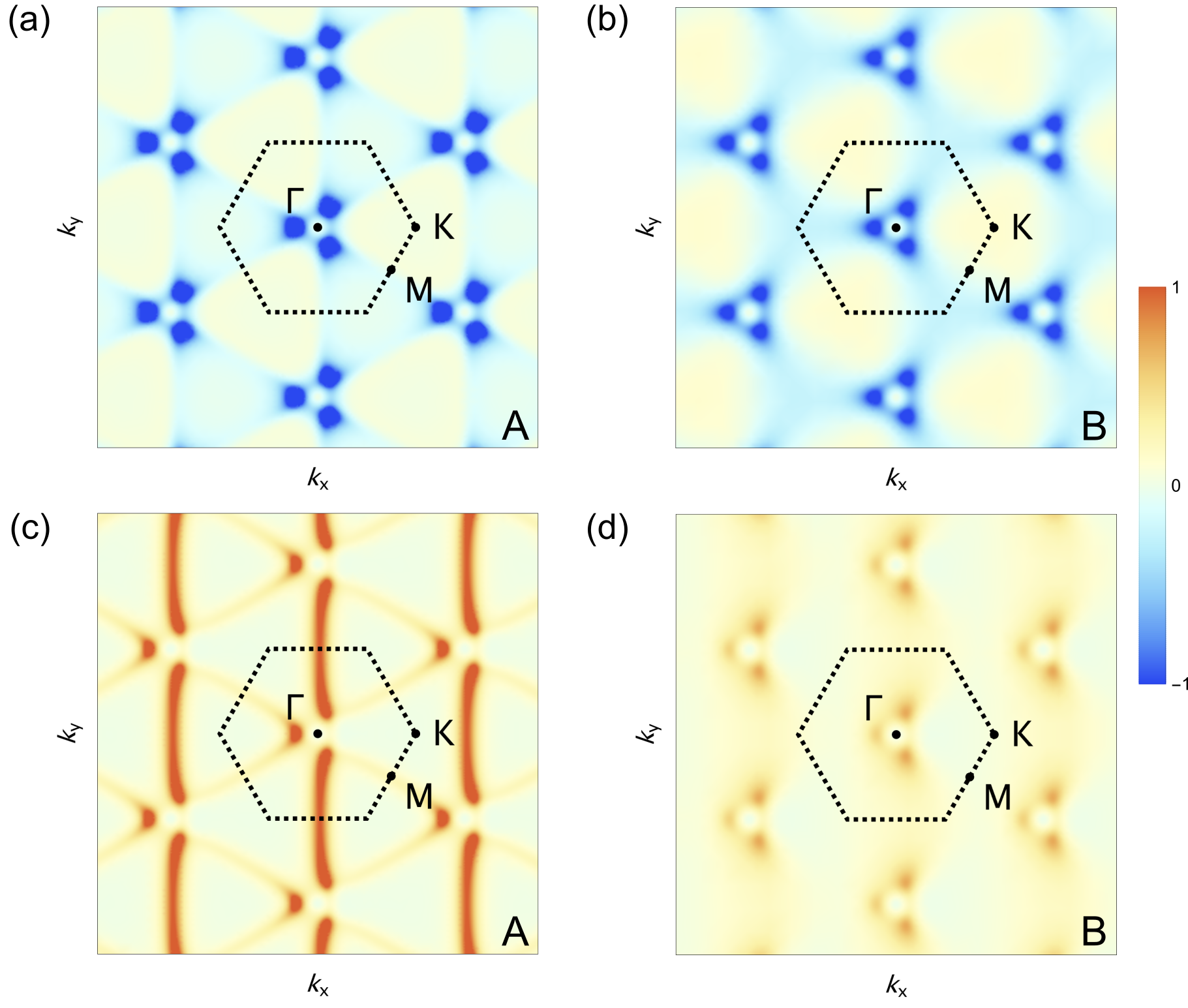
B.5 Berry curvature and quantum metric for the two-band model at $k_{z}=\pi/2$

For the parameter sets A and B we show the Berry curvature and quantum metric at $k_{z}=\pi/2$ in Fig. 4. Besides the divergence of Berry curvature and quantum metric at the Weyl points, both quantities exhibit larger values for the parameter set A, i.e., the one with the smaller gap on $\Gamma$-A. Notably, albeit the localization of the weight in k space strongly differs between models A and B, as seen when comparing (c) to (d), the integrated values are of the same order of magnitude. Specifically, integrating the metric on the plane shown in Fig. 4 (c)[d] yields $\int\frac{d^{2}\mathbf{k}}{V}g^{xx}_{-}(\mathbf{k})=0.80\,\,[0.74]$ with $V=8\pi^{2}/\sqrt{3}$. For the Berry curvature the values are identical, because the integral over the plane shown in Fig. 4 (a,b) equals the Chern number of $\nu=-1$.

Refer to caption
Figure 4: Berry curvature $\Omega^{xy}_{-}$ (a,b) and quantum metric $g^{xx}_{-}$ (c,d) at $k_{z}=\pi/2$ for the parameter sets A and B of the two-band model.

B.6 Effect of the parameters on several model properties

We give several relations between basic band structure properties and the five model parameters, the $\mathbf{a}_{1}$-$\mathbf{a}_{2}$-plane hoppings $t^{d}_{xy\pm}$ and $\tilde{t}^{d}_{xy}$ and the out-of-plane hoppings $t^{d}_{z\pm}$. Note that $\tilde{t}^{d}_{xy}$ is in general complex, whereas the other parameters are real. We focus on the high-symmetry points $\Gamma=(0,0,0)$, $M=(\pi,-\pi/\sqrt{3},0)$, $K=(4\pi/3,0,0)$, $A=(0,0,\pi)$, $L=(\pi,-\pi/\sqrt{3},\pi)$, and $H=(4\pi/3,0,\pi)$.

B.6.1 Size of band gaps at high-symmetry points and on the $\Gamma$-A line

We define the size of the band gaps as $\Delta_{\mathbf{k}}=E_{+}(\mathbf{k})-E_{-}(\mathbf{k})=2d(\mathbf{k})$ and obtain

$\displaystyle\Delta_{\Gamma}=0\,,\hskip 14.22636pt\Delta_{M}=4|\tilde{t}^{d}_{xy}|\,,\hskip 14.22636pt\Delta_{K}=3\sqrt{3}|t^{d}_{xy-}|\,,\hskip 14.22636pt\Delta_{A}=0\,,\hskip 14.22636pt\Delta_{L}=4|\tilde{t}^{d}_{xy}|\,,\hskip 14.22636pt\Delta_{H}=3\sqrt{3}|t^{d}_{xy-}|\,.$ (23)

We see that $\Delta_{\Gamma}=\Delta_{A}=0$ as expected. Furthermore, $\Delta_{M}=\Delta_{L}$ and $\Delta_{K}=\Delta_{H}$. The splitting on the symmetry line $\Gamma$-A, that is $\mathbf{k}=(0,0,k_{z})$ is given by

$\displaystyle\Delta_{\Gamma\text{-}A}=2|t^{d}_{z-}\sin(\mathbf{k}\cdot\mathbf{a}_{3})|\,,$ (24)

with maximal value $\Delta^{\text{max}}_{\Gamma\text{-}A}=2|t^{d}_{z-}|$ for $k_{z}=\pi/2$.

B.6.2 Band curvature at $\Gamma$ and A in various directions

The momentum expansion of the two bands at $\Gamma=(0,0,0)$ in direction $\mathbf{v_{\Gamma\text{-}M}}=(M-\Gamma)/|M-\Gamma|=(\sqrt{3}/2,-1/2,0)$ and $\mathbf{v_{G\text{-}K}}=(K-\Gamma)/|K-\Gamma|=(1,0,0)$ reads

$\displaystyle E_{+}\big{(}k\,\mathbf{v_{\Gamma\text{-}M}}\big{)}=E_{+}\big{(}k\,\mathbf{v_{\Gamma\text{-}K}}\big{)}=\Big{(}3t^{d}_{xy+}+t^{d}_{z+}-\mu_{d}\Big{)}+\frac{3}{8}\Big{(}|\tilde{t}^{d}_{xy}|-2t^{d}_{xy+}\Big{)}\,k^{2}+\mathcal{O}(k^{3})\,,$ (25)
$\displaystyle E_{-}\big{(}k\,\mathbf{v_{\Gamma\text{-}M}}\big{)}=E_{-}\big{(}k\,\mathbf{v_{\Gamma\text{-}K}}\big{)}=\Big{(}3t^{d}_{xy+}+t^{d}_{z+}-\mu_{d}\Big{)}-\frac{3}{8}\Big{(}|\tilde{t}^{d}_{xy}|+2t^{d}_{xy+}\Big{)}\,k^{2}+\mathcal{O}(k^{3})\,.$ (26)

The momentum expansion of the two bands at $A=(0,0,\pi)$ in direction $\mathbf{v_{A\text{-}L}}=(L-A)/|L-A|=(\sqrt{3}/2,-1/2,0)$ and $\mathbf{v_{A\text{-}H}}=(H-A)/|H-A|=(1,0,0)$ reads

$\displaystyle E_{+}\big{(}k\,\mathbf{v_{A\text{-}L}}\big{)}=E_{+}\big{(}k\,\mathbf{v_{A\text{-}H}}\big{)}=\Big{(}3t^{d}_{xy+}-t^{d}_{z+}-\mu_{d}\Big{)}+\frac{3}{8}\Big{(}|\tilde{t}^{d}_{xy}|-2t^{d}_{xy+}\Big{)}\,k^{2}+\mathcal{O}(k^{3})\,,$ (27)
$\displaystyle E_{-}\big{(}k\,\mathbf{v_{A\text{-}L}}\big{)}=E_{-}\big{(}k\,\mathbf{v_{A\text{-}H}}\big{)}=\Big{(}3t^{d}_{xy+}-t^{d}_{z+}-\mu_{d}\Big{)}-\frac{3}{8}\Big{(}|\tilde{t}^{d}_{xy}|+2t^{d}_{xy+}\Big{)}\,k^{2}+\mathcal{O}(k^{3})\,.$ (28)

We read off six different scenarios. If $|\tilde{t}^{d}_{xy}|=2|t^{d}_{xy+}|$ or $|\tilde{t}^{d}_{xy}|=-2|t^{d}_{xy+}|$, the upper or the lower band remains flat. We conclude the following trends

$\displaystyle E_{+}\,\text{with positive curvature}\hskip 28.45274pt$ $\displaystyle\text{if}\hskip 28.45274pt|\tilde{t}^{d}_{xy}|>\phantom{-}2t^{d}_{xy+}\,,$ (29)
$\displaystyle E_{+}\,\text{with negative curvature}\hskip 28.45274pt$ $\displaystyle\text{if}\hskip 28.45274pt|\tilde{t}^{d}_{xy}|<\phantom{-}2t^{d}_{xy+}\,,$ (30)
$\displaystyle E_{-}\,\text{with positive curvature}\hskip 28.45274pt$ $\displaystyle\text{if}\hskip 28.45274pt|\tilde{t}^{d}_{xy}|<-2t^{d}_{xy+}\,,$ (31)
$\displaystyle E_{-}\,\text{with negative curvature}\hskip 28.45274pt$ $\displaystyle\text{if}\hskip 28.45274pt|\tilde{t}^{d}_{xy}|>-2t^{d}_{xy+}\,.$ (32)

We see that the trends depend on the relative size of $|\tilde{t}^{d}_{xy}|$ and $|t^{d}_{xy+}|$ as well as the sign of $t^{d}_{xy+}$. We summarize the result in Tab. 2.

$E_{+}$ $E_{-}$ Conditions
$\nearrow$ $\nearrow$ $2|t^{d}_{xy+}|>|\tilde{t}^{d}_{xy}|$   and   $t^{d}_{xy+}<0$
$\searrow$ $\searrow$ $2|t^{d}_{xy+}|>|\tilde{t}^{d}_{xy}|$   and   $t^{d}_{xy+}>0$
$\nearrow$ $\searrow$ $|\tilde{t}^{d}_{xy}|>2|t^{d}_{xy+}|$
Table 2: The parameter dependence of the curvature trends at $\Gamma$ and A in direction $M,K$ and $L,H$, respectively. $\nearrow$ indicates a positive curvature. $\searrow$ indicates a negative curvature. The missing combination ($\searrow$ $\nearrow$) is inconsistent with the fixed definition of the lower and upper band and, thus, left out.

B.6.3 Lower-band shift at K and H with respect to $\Gamma$

The energy of the lower band at high-symmetry points K and H with respect to $\Gamma$ is given by

$\displaystyle E_{-}(K)-E_{-}(\Gamma)=-\frac{3\sqrt{3}}{2}|t^{d}_{xy-}|-\frac{9}{2}t^{d}_{xy+}\,,$ (37)
$\displaystyle E_{-}(H)-E_{-}(\Gamma)=-\frac{3\sqrt{3}}{2}|t^{d}_{xy-}|-\frac{9}{2}t^{d}_{xy+}-2t^{d}_{z+}\,.$ (38)

Appendix C Four-band model

C.1 Sublattice hopping in the four-band model

We give the explicit form of the sublattice hopping of the four-band model in Eq. (5). They are

$\displaystyle H_{dp}(\mathbf{k})=\mathrm{e}^{i\mathbf{k}\cdot\big{(}(\mathbf{a}_{1}+2\mathbf{a}_{2})/3+z\,\mathbf{a}_{3}\big{)}}\begin{pmatrix}H^{dp}_{11}(\mathbf{k})&H^{dp}_{12}(\mathbf{k})\\[2.84526pt] H^{dp}_{21}(\mathbf{k})&H^{dp}_{22}(\mathbf{k})\end{pmatrix},$ (39)

with the 1b Wyckoff position $(\mathbf{a}_{1}+2\mathbf{a}_{2})/3+z\,\mathbf{a}_{3}$ and

$\displaystyle H^{dp}_{11}(\mathbf{k})$ $\displaystyle=(t^{dp}_{xy}+t^{dp}_{xyz}\mathrm{e}^{i\mathbf{k}\cdot\mathbf{a}_{3}})\Big{[}1+\mathrm{e}^{-i\mathbf{k}\cdot\mathbf{a}_{2}}+\mathrm{e}^{-i\mathbf{k}\cdot(\mathbf{a}_{1}+\mathbf{a}_{2})}\Big{]}\,,$ (40)
$\displaystyle H^{dp}_{22}(\mathbf{k})$ $\displaystyle=H^{dp}_{11}(-\mathbf{k})^{*}\,,$ (41)
$\displaystyle H^{dp}_{12}(\mathbf{k})$ $\displaystyle=\left(\tilde{t}^{dp}_{xy}+\tilde{t}^{dp}_{xyz}\mathrm{e}^{i\mathbf{k}\cdot\mathbf{a}_{3}}\right)\Big{[}1+\mathrm{e}^{i\frac{2\pi}{3}}\mathrm{e}^{-i\mathbf{k}\cdot\mathbf{a}_{2}}+\mathrm{e}^{-i\frac{2\pi}{3}}\mathrm{e}^{-i\mathbf{k}\cdot(\mathbf{a}_{1}+\mathbf{a}_{2})}\Big{]}\,,$ (42)
$\displaystyle H^{dp}_{21}(\mathbf{k})$ $\displaystyle=H^{dp}_{12}(-\mathbf{k})^{*}\,.$ (43)

Note, the relative height difference between the 1a and 1b Wyckoff positions, denoted as $z$ in Eq. (39), does not affect the band structure. For the present work the exact value of $z$ does not affect the results, because all considered geometric quantities are restricted to derivatives in the $k_{x}$-$k_{y}$-plane.

C.2 Symmetries and basis convention

The second pair of bands described by $H_{p}(\mathbf{k})$ obeys by itself the same symmetry representation as $H_{d}(\mathbf{k})$, but since the 1b Wyckoff position is not invariant under $C_{3}$, the application of $C_{3}$ moves the site into a neighboring unit cell. Thus, the unitary representation $U_{C_{3}}$ contains a factor of $\mathrm{e}^{i\mathbf{k}\cdot(\mathbf{a}_{1}+\mathbf{a}_{2})}$. Yet, once represented in the basis convention introduced by the Fourier transform in Eq. (12), this phase cancels and one finds

$\displaystyle U^{p}_{C_{3}}=\begin{pmatrix}\mathrm{e}^{i\frac{2\pi}{3}}&0\\[2.84526pt] 0&\mathrm{e}^{-i\frac{2\pi}{3}}\end{pmatrix}$ (44)

leading to the definition

$\displaystyle U_{C_{3}}=\begin{pmatrix}U^{d}_{C_{3}}&0\\[2.84526pt] 0&U^{p}_{C_{3}}\end{pmatrix},$ (45)

which is then a symmetry of the four-band model $H_{4\times 4}(\mathbf{k})$ given in Eq. (5). Time-reversal symmetry is local in real space, and hence is the same for the states corresponding to 1a and 1b Wyckoff positions.

C.3 Real-space version of the tight-binding Hamiltonian

The tight-binding Hamiltonian defined in Eq. (5) is Fourier transformed to real space via Eq. (12). The annihiliation operators for the d and p orbitals are denoted by $\hat{d}_{\nu}$ and $\hat{p}_{\nu}$ with $\nu=1,2$. The d and p orbitals are located at $\bm{\rho}_{d}=(0,0,0)$ and $\bm{\rho}_{p}=(\mathbf{a}_{1}+2\mathbf{a}_{2})/3+z\mathbf{a}_{3}=(1/2,1/2\sqrt{3},z)$ in the unit cell. The Fourier transform of $H_{d}(\mathbf{k})$ is already given in Eq. (13). The Fourier transform of $H_{p}(\mathbf{k})$ is equivalent to those of $H_{d}(\mathbf{k})$ with $d$ replaced by $p$. We give the remaining expressions of $H_{dp}(\mathbf{k})$,

$\displaystyle\hat{H}^{dp}_{11}=\sum_{j}\Bigg{[}\,$ $\displaystyle t^{dp}_{xy}\,\Big{(}\hat{d}^{\dagger}_{j,1}\hat{p}^{\phantom{\dagger}}_{j,1}+\hat{d}^{\dagger}_{j+j_{1}+j_{2},1}\hat{p}^{\phantom{\dagger}}_{j,1}+\hat{d}^{\dagger}_{j+j_{2},1}\hat{p}^{\phantom{\dagger}}_{j,1}\Big{)}$
$\displaystyle+t^{dp}_{xyz}\,\Big{(}\hat{d}^{\dagger}_{j,1}\hat{p}^{\phantom{\dagger}}_{j+j_{3},1}+\hat{d}^{\dagger}_{j+j_{1}+j_{2},1}\hat{p}^{\phantom{\dagger}}_{j+j_{3},1}+\hat{d}^{\dagger}_{j+j_{2},1}\hat{p}^{\phantom{\dagger}}_{j+j_{3},1})\Big{)}\Bigg{]}\,,$ (46)
$\displaystyle\hat{H}^{dp}_{22}=\sum_{j}\Bigg{[}\,$ $\displaystyle\big{(}t^{dp}_{xy}\big{)}^{*}\,\Big{(}\hat{d}^{\dagger}_{j,2}\hat{p}^{\phantom{\dagger}}_{j,2}+\hat{d}^{\dagger}_{j+j_{1}+j_{2},2}\hat{p}^{\phantom{\dagger}}_{j,2}+\hat{d}^{\dagger}_{j+j_{2},2}\hat{p}^{\phantom{\dagger}}_{j,2}\Big{)}$
$\displaystyle+\big{(}t^{dp}_{xyz}\big{)}^{*}\,\Big{(}\hat{d}^{\dagger}_{j,2}\hat{p}^{\phantom{\dagger}}_{j+j_{3},2}+\hat{d}^{\dagger}_{j+j_{1}+j_{2},2}\hat{p}^{\phantom{\dagger}}_{j+j_{3},2}+\hat{d}^{\dagger}_{j+j_{2},2}\hat{p}^{\phantom{\dagger}}_{j+j_{3},2})\Big{)}\Bigg{]}\,,$ (47)
$\displaystyle\hat{H}^{dp}_{12}=\sum_{j}\Bigg{[}\,$ $\displaystyle\tilde{t}^{dp}_{xy}\,\Big{(}\hat{d}^{\dagger}_{j,1}\hat{p}^{\phantom{\dagger}}_{j,2}+e^{i2\pi/3}\hat{d}^{\dagger}_{j+j_{2},1}\hat{p}^{\phantom{\dagger}}_{j,2}+e^{-i2\pi/3}\,\hat{d}^{\dagger}_{j+j_{1}+j_{2},1}\hat{p}^{\phantom{\dagger}}_{j,2}\Big{)}$
$\displaystyle+\tilde{t}^{dp}_{xyz}\,\Big{(}\hat{d}^{\dagger}_{j,1}\hat{p}^{\phantom{\dagger}}_{j+j_{3},2}+e^{i2\pi/3}\hat{d}^{\dagger}_{j+j_{2},1}\hat{p}^{\phantom{\dagger}}_{j+j_{3},2}+e^{-i2\pi/3}\hat{d}^{\dagger}_{j+j_{1}+j_{2},1}\hat{p}^{\phantom{\dagger}}_{j+j_{3},2}\Big{)}\Bigg{]}\,,$ (48)

and $\hat{H}^{dp}_{21}=(\hat{H}^{dp}_{12})^{\dagger}$.

C.4 Quantum geometry of four-band model

In contrast to the two-band model, a closed analytic formula is hard to obtain. Thus, a numerical evaluation is most promising. We make use of the projector formalism, which does not suffer from numerical artifacts due to the momentum-dependent gauge ambiguity of the cell-periodic Bloch wave function $|u_{n}(\mathbf{k})\rangle$ of each band $n$. We label the bands from 1 to 4 starting from the band of highest energy. For a fixed momentum, we obtain the complex four vector $|u_{n}(\mathbf{k})\rangle$ and construct the respective projector, a $4\times 4$ matrix,

$\displaystyle P_{n}(\mathbf{k})=|u_{n}(\mathbf{k})\rangle\langle u_{n}(\mathbf{k})|\,,$ (49)

which is gauge invariant since an arbitrary phase $\phi_{\mathbf{k}}$ in the transformation $|u_{n}(\mathbf{k})\rangle\rightarrow e^{i\phi_{\mathbf{k}}}|u_{n}(\mathbf{k})\rangle$ cancels due to its appearance in both the bra and ket. The projector is not well-defined at the momenta of band touching. In addition to the four projectors of each band we construct the projector of the two combined sets of isolated bands, which are present for the considered parameter set, that is,

$\displaystyle P_{12}(\mathbf{k})=P_{1}(\mathbf{k})+P_{2}(\mathbf{k})\,,\hskip 28.45274ptP_{34}(\mathbf{k})=P_{3}(\mathbf{k})+P_{4}(\mathbf{k})\,.$ (50)

This projector on the subsystem is gauge invariant under $U(2)$ gauge transformations. They are well-defined for all momenta since no band crossings between the two isolated subsystems occur. Due to its gauge invariance the numerical evaluation of derivatives of the projectors are straightforward. We use

$\displaystyle\partial_{x}P_{j}(\mathbf{k})=\frac{1}{2\delta}\big{[}P_{j}(k_{x}+\delta,k_{y},k_{z})-P_{j}(k_{x}-\delta,k_{y},k_{z})\big{]}$ (51)

and accordingly for $\partial_{y}P_{j}(\mathbf{k})$ or arbitrary directional derivatives for all projectors $j$ defined above. We used $\delta=10^{-4}$ in our calculation. To check numerical accuracy we checked the projector identities $P_{n}(\mathbf{k})P_{m}(\mathbf{k})=\delta_{nm}P_{n}(\mathbf{k})$ for $n=1,2,3,4$ as well as $\big{(}\partial_{x}P_{j}(\mathbf{k})\big{)}P_{j}(\mathbf{k})+P_{j}(\mathbf{k})\big{(}\partial_{x}P_{j}(\mathbf{k})\big{)}=0$ for all projectors. We calculate the quantum metric and Berry curvature via

$\displaystyle g^{\alpha\beta}_{j}(\mathbf{k})=\frac{1}{2}\text{Tr}\bigg{[}\partial_{\alpha}P_{j}(\mathbf{k})\,\partial_{\beta}P_{j}(\mathbf{k})\bigg{]}\,,$ (52)
$\displaystyle\Omega^{\alpha\beta}_{j}(\mathbf{k})=i\,\text{Tr}\bigg{[}P_{j}(\mathbf{k})\bigg{(}\partial_{\alpha}P_{j}(\mathbf{k})\partial_{\beta}P_{j}(\mathbf{k})-\partial_{\beta}P_{j}(\mathbf{k})\partial_{\alpha}P_{j}(\mathbf{k})\bigg{)}\bigg{]}\,.$ (53)

We focus on the quantum metric in $x$-direction $g^{xx}_{j}(\mathbf{k})$ and the Berry curvature in $x$-$y$ plane $\Omega^{xy}_{j}(\mathbf{k})$. Note that the quantum metric is not additive in general in contrast to the Berry curvature. We have

$\displaystyle g^{xx}_{12}(\mathbf{k})=g^{xx}_{1}(\mathbf{k})+g^{xx}_{2}(\mathbf{k})+\text{Tr}\big{[}\partial_{x}P_{1}(\mathbf{k})\,\,\partial_{x}P_{2}(\mathbf{k})\big{]}\,,$ (54)
$\displaystyle\Omega^{xy}_{12}(\mathbf{k})=\Omega^{xy}_{1}(\mathbf{k})+\Omega^{xy}_{2}(\mathbf{k})\,.$ (55)

Beside the physical insight these equations can also used as consistency checks. We show $g^{xx}_{2}(\mathbf{k})$ in Fig. 2 (c) and $g^{xx}_{12}(\mathbf{k})$ in Fig. 2 (d). We show $\Omega^{xy}_{2}(\mathbf{k})$ in Fig. 2 (f) and $\Omega^{xy}_{12}(\mathbf{k})$ in Fig. 2 (h).

Appendix D Analysis of flat-bands within the two-band model

D.1 Derivation of the flat-band conditions

We present a strategy to systematically derive the conditions to flatten one of the two bands. Taking the particular form of the eigenvalues in Eq. (18), we obtain a flat band for one of the two bands when the condition

$\displaystyle d(\mathbf{k})^{2}=d_{x}^{2}(\mathbf{k})+d_{y}^{2}(\mathbf{k})+d_{z}^{2}(\mathbf{k})=(d_{0}(\mathbf{k})+c_{0})^{2}$ (56)

is fulfilled for a momentum-constant $c_{0}$. In this case, we have

$\displaystyle E_{+}(\mathbf{k})=2d_{0}(\mathbf{k})+c_{0},\hskip 28.45274pt$ $\displaystyle E_{-}(\mathbf{k})=-c_{0}$ for $\displaystyle d_{0}(\mathbf{k})+c_{0}>0,$ (57)
$\displaystyle E_{+}(\mathbf{k})=-c_{0},$ $\displaystyle E_{-}(\mathbf{k})=2d_{0}(\mathbf{k})+c_{0}\hskip 28.45274pt$ for $\displaystyle d_{0}(\mathbf{k})+c_{0}<0.$ (58)

Thus, we obtain conditions on the parameters in the Hamiltonian by enforcing

$\displaystyle f(\mathbf{k})=d_{x}^{2}(\mathbf{k})+d_{y}^{2}(\mathbf{k})+d_{z}^{2}(\mathbf{k})-(d_{0}(\mathbf{k})+c_{0})^{2}=0$ (59)

for all relevant momenta $\mathbf{k}$, for which the band should be flat. If we assume that $f(\mathbf{k})$ is an analytic function, which is fulfilled for tight-binding Hamiltonians, we can alternatively Taylor expand $f(\mathbf{k})$ around a specific momentum with finite band gap and solve the (generically infinite) set of equations enforcing the expansion coefficients to vanish.

D.2 Compact localized states

Without loss of generality, let us assume that the lower band is flat in the following. Under the flat-band condition (59) the eigenvector given in Eqs. (20) takes the form

$\displaystyle\bm{v}_{-}(\mathbf{k})=\frac{1}{\alpha_{\mathbf{k}}}\begin{pmatrix}d_{z}(\mathbf{k})-d_{0}(\mathbf{k})-c_{0}\\[5.69054pt] d_{x}(\mathbf{k})+id_{y}(\mathbf{k})\end{pmatrix}$ (60)

with

$\displaystyle\alpha_{\mathbf{k}}=\sqrt{2}\sqrt{(d_{0}(\mathbf{k})+c_{0})(d_{0}(\mathbf{k})+d_{z}(\mathbf{k})+c_{0})}\,.$ (61)

Following Ref. [86] and using the particular property of non-interacting tight-binding Hamiltonians, we note that each component of $\alpha_{\mathbf{k}}\bm{v}_{-}(\mathbf{k})$ is a finite polynomial of $\text{Exp}\big{(}i\mathbf{k}\cdot\sum_{l}m_{l}\mathbf{a}_{l}\big{)}$. The corresponding compact localized state is given by [86]

$\displaystyle|\chi_{\mathbf{R}}\rangle=\sum_{\mathbf{R}^{\prime}}w^{1}_{\mathbf{R},\mathbf{R}^{\prime}}|\mathbf{R}^{\prime},d_{1}\rangle+\sum_{\mathbf{R}^{\prime}}w^{2}_{\mathbf{R},\mathbf{R}^{\prime}}|\mathbf{R}^{\prime},d_{2}\rangle$ (62)

with

$\displaystyle w_{\mathbf{R},\mathbf{R}^{\prime}}=\frac{c_{\chi}}{\sqrt{N_{c}}}\sum_{\mathbf{k}}\alpha_{\mathbf{k}}\,e^{i\mathbf{k}\cdot(\mathbf{R}^{\prime}-\mathbf{R})}\bm{v}_{-}(\mathbf{k})\,,$ (63)

where $w^{\alpha}_{\mathbf{R},\mathbf{R}^{\prime}}$ denotes the component of $w_{\mathbf{R},\mathbf{R}^{\prime}}$ for the two distinct states $d_{1}$ and $d_{2}$. $|\mathbf{R},d_{\alpha}\rangle$ denotes the state of $\alpha=1,2$ within the unit cell labeled by $\mathbf{R}$. $N_{c}$ is the number of unit cells and $c_{\chi}$ is the normalization constant. The compact localized state (62) is an eigenfunction of the flat band. Note that $|\chi_{\mathbf{R}}\rangle$ for different $\mathbf{R}$ are in general not orthogonal. The $N$ shifted copies of $|\chi_{\mathbf{R}}\rangle$ not necessarily form a complete basis when $\alpha_{\mathbf{k}}=0$ for some momentum $\mathbf{k}$. Flat bands where the compact localized states cannot span the entire flat band was dubbed singular flat band [86].

Refer to caption
Figure 5: Band structure fulfilling the flat-band conditions.

D.3 Application to our proposed two-band model

Considering the Hamiltonian defined in Eq. (1), we construct

$\displaystyle d_{0}(\mathbf{k})=\frac{1}{2}\big{(}H_{11}(\mathbf{k})+H_{22}(\mathbf{k})\big{)}\,,$ (64)
$\displaystyle d_{x}(\mathbf{k})=\frac{1}{2}\big{(}H_{12}(\mathbf{k})+H_{21}(\mathbf{k})\big{)}\,,$ (65)
$\displaystyle d_{y}(\mathbf{k})=\frac{i}{2}\big{(}H_{12}(\mathbf{k})-H_{21}(\mathbf{k})\big{)}\,,$ (66)
$\displaystyle d_{z}(\mathbf{k})=\frac{1}{2}\big{(}H_{11}(\mathbf{k})-H_{22}(\mathbf{k})\big{)}\,.$ (67)

We are interest in a flat band in the $x$-$y$ plane and fix $k_{z}=0$. Following the procedure as described above, we obtain four sets of flat-band conditions different in the relative sign only,

$\displaystyle\Bigl{\{}t^{d}_{xy+}=-\frac{1}{2}|\tilde{t}^{d}_{xy}|\,,\hskip 28.45274pt$ $\displaystyle t^{d}_{xy-}=-\frac{\sqrt{3}}{2}|\tilde{t}^{d}_{xy}|\,,$ $\displaystyle c_{0}=\phantom{-}\frac{3}{2}|\tilde{t}^{d}_{xy}|-t^{d}_{z+}+\mu_{d}\Bigl{\}}$ (68)
$\displaystyle\Bigl{\{}t^{d}_{xy+}=-\frac{1}{2}|\tilde{t}^{d}_{xy}|\,,$ $\displaystyle t^{d}_{xy-}=\phantom{-}\frac{\sqrt{3}}{2}|\tilde{t}^{d}_{xy}|\,,$ $\displaystyle c_{0}=\phantom{-}\frac{3}{2}|\tilde{t}^{d}_{xy}|-t^{d}_{z+}+\mu_{d}\Bigl{\}}$ (69)
$\displaystyle\Bigl{\{}t^{d}_{xy+}=\phantom{-}\frac{1}{2}|\tilde{t}^{d}_{xy}|\,,$ $\displaystyle t^{d}_{xy-}=-\frac{\sqrt{3}}{2}|\tilde{t}^{d}_{xy}|\,,\hskip 28.45274pt$ $\displaystyle c_{0}=-\frac{3}{2}|\tilde{t}^{d}_{xy}|-t^{d}_{z+}+\mu_{d}\Bigl{\}}$ (70)
$\displaystyle\Bigl{\{}t^{d}_{xy+}=\phantom{-}\frac{1}{2}|\tilde{t}^{d}_{xy}|\,,$ $\displaystyle t^{d}_{xy-}=\phantom{-}\frac{\sqrt{3}}{2}|\tilde{t}^{d}_{xy}|\,,$ $\displaystyle c_{0}=-\frac{3}{2}|\tilde{t}^{d}_{xy}|-t^{d}_{z+}+\mu_{d}\Bigl{\}}$ (71)

The dispersion in the $x$-$y$ plane remains flat for any $k_{z}$ for arbitrary $t^{d}_{z+}$. A finite $t^{d}_{z-}$ gaps the quadratic band touching at $k_{x}=k_{y}=0$ for any $k_{z}\neq 0,\pi$ and breaks the flat-band conditions leading to a dispersive lower band in the $x$-$y$ plane, which we do not further consider. We give the following concrete example by choosing the parameters

$\displaystyle\Bigl{\{}t^{d}_{xy+}=-\frac{1}{4}\,,\hskip 28.45274ptt^{d}_{xy-}=-\frac{\sqrt{3}}{4}\,,\hskip 28.45274pt\tilde{t}^{d}_{xy}=-\frac{1}{2}\,,\hskip 28.45274ptt^{d}_{z+}=-\frac{1}{2}\,,\hskip 28.45274ptt^{d}_{z-}=0\,,\hskip 28.45274pt\mu_{d}=-\frac{1}{4}\Bigl{\}}\,,$ (72)

where we obtain a flat lower band at energy $E_{-}(\mathbf{k})=-1$ for $k_{z}=0$ and $E_{-}(\mathbf{k})=0$ for $k_{z}=\pi$ with band gap $E_{+}(\mathbf{k})-E_{-}(\mathbf{k})=2$ at momentum $M=(\pi,-\pi/\sqrt{3},0)$. The Hamiltonian is explicitly given by $H(\mathbf{k})=d_{0}(\mathbf{k})+d_{x}(\mathbf{k})\sigma_{x}+d_{y}(\mathbf{k})\sigma_{y}+d_{z}(\mathbf{k})\sigma_{z}$ with

$\displaystyle d_{0}(\mathbf{k})=\frac{1}{4}\Big{(}1-\cos\big((\mathbf{a}_{1}+\mathbf{a}_{2})\cdot\mathbf{k}\big{missing})-\cos\big(\mathbf{a}_{1}\cdot\mathbf{k}\big{missing})-\cos\big(\mathbf{a}_{2}\cdot\mathbf{k}\big{missing})-2\cos\big(\mathbf{a}_{3}\cdot\mathbf{k}\big{missing})\Big{)}\,,$ (73)
$\displaystyle d_{x}(\mathbf{k})=\frac{1}{4}\Big{(}\cos\big((\mathbf{a}_{1}+\mathbf{a}_{2})\cdot\mathbf{k}\big{missing})-2\cos\big(\mathbf{a}_{1}\cdot\mathbf{k}\big{missing})+\cos\big(\mathbf{a}_{2}\cdot\mathbf{k}\big{missing})\Big{)}\,,$ (74)
$\displaystyle d_{y}(\mathbf{k})=\frac{\sqrt{3}}{4}\Big{(}\cos\big((\mathbf{a}_{1}+\mathbf{a}_{2})\cdot\mathbf{k}\big{missing})-\cos\big(\mathbf{a}_{2}\cdot\mathbf{k}\big{missing})\Big{)}\,,$ (75)
$\displaystyle d_{z}(\mathbf{k})=\frac{\sqrt{3}}{4}\Big{(}\sin\big((\mathbf{a}_{1}+\mathbf{a}_{2})\cdot\mathbf{k}\big{missing})-\sin\big(\mathbf{a}_{1}\cdot\mathbf{k}\big{missing})-\sin\big(\mathbf{a}_{2}\cdot\mathbf{k}\big{missing})\Big{)}\,.$ (76)

The dispersion is shown in Fig. 5 (b). The compact localized eigenfunction with eigenvalue $E_{\text{flat}}(\mathbf{k})=-\cos\big(\mathbf{a}_{3}\cdot\mathbf{k}\big{missing})$ constructed as described above reads

$\displaystyle\bm{v}_{\text{flat}}(\mathbf{k})=\frac{1}{\alpha_{\mathbf{k}}}\Biggr{[}\begin{pmatrix}-3\\ 0\end{pmatrix}$ $\displaystyle+\begin{pmatrix}w^{*}\\ w\end{pmatrix}e^{i\mathbf{k}\cdot(\mathbf{a}_{1}+\mathbf{a}_{2})}+\begin{pmatrix}w\\ w\end{pmatrix}e^{-i\mathbf{k}\cdot(\mathbf{a}_{1}+\mathbf{a}_{2})}$
$\displaystyle+\begin{pmatrix}w\\ w^{*}\end{pmatrix}e^{i\mathbf{k}\cdot\mathbf{a}_{2}}+\begin{pmatrix}w^{*}\\ w^{*}\end{pmatrix}e^{-i\mathbf{k}\cdot\mathbf{a}_{2}}+\begin{pmatrix}w\\ -1\end{pmatrix}e^{i\mathbf{k}\cdot\mathbf{a}_{1}}+\begin{pmatrix}w^{*}\\ -1\end{pmatrix}e^{-i\mathbf{k}\cdot\mathbf{a}_{1}}\Biggr{]}$ (77)

with $w=\frac{1}{2}(1+i\sqrt{3})=-e^{-i2\pi/3}$ and its complex conjugate $w^{*}$. The normalization is

$\displaystyle\alpha_{\mathbf{k}}^{2}=2\,\bigg{(}-3+\cos\big((\mathbf{a}_{1}+\mathbf{a}_{2})\cdot\mathbf{k}\big{missing})+\cos\big(\mathbf{a}_{1}\cdot\mathbf{k}\big{missing})+\cos\big(\mathbf{a}_{2}\cdot\mathbf{k}\big{missing})\bigg{)}$
$\displaystyle\hskip 56.9055pt\times\bigg{(}-3+\cos\big((\mathbf{a}_{1}+\mathbf{a}_{2})\cdot\mathbf{k}\big{missing})+\cos\big(\mathbf{a}_{1}\cdot\mathbf{k}\big{missing})+\cos\big(\mathbf{a}_{2}\cdot\mathbf{k}\big{missing})$
$\displaystyle\hskip 113.81102pt-\sqrt{3}\Big{(}\sin\big(\mathbf{a}_{1}\cdot\mathbf{k}\big{missing})+\sin\big(\mathbf{a}_{2}\cdot\mathbf{k}\big{missing})-\sin\big((\mathbf{a}_{1}+\mathbf{a}_{2})\cdot\mathbf{k}\big{missing})\Big{)}\bigg{)}$ (78)

which vanishes at $\Gamma=(0,0,0)$. We see that the eigenvector is of the form given in Eq. (63) so that we can read of the compact localized state (CLS) given in Eq. (62). One particular CLS is centered on one site on the triangular lattice and its six neighbors with the corresponding weights for the two orbitals. The localization crucially rely on the destructive interference between the two orbitals as sketched in Fig. 5 (a), where we give the weights and the hopping amplitudes, explicitly. Each bond takes the form of the well-known Creutz ladder [29], a frustrated lattice in one dimension, so that we can interpret the model as two-dimensional version thereof.