What about translation? New coding system for content analysis on the perception of literary translation around the political transformation in 1989 in Hungary as a classification problem on an unbalanced dataset

Abstract

To track trends in the perception of literary translation around the political transformation in 1989 in Hungary, a coding system was developed on the paragraphs of the 1980–1999 issues of the literary journal Alföld. This paper describes how we trained BERT models to carry over the coding system to the 1980–1999 issues of the literary journal Nagyvilág. We use extensive hyperparameter tuning, loss functions robust to label unbalance, 10-fold cross-validation for precise evaluations and a model ensemble for prediction, manual validation on the predict set, a new calibration method to better predict label counts for sections of the Nagyvilág corpus, and to study the relations between labels, we construct label relation networks.

Keywords BERT $\cdot$ calibration $\cdot$ coding system $\cdot$ domain shift $\cdot$ ensemble learning $\cdot$ Literary Translation Studies $\cdot$ semantic network $\cdot$ social perception $\cdot$ unbalanced dataset

1 Introduction

1.1 Research problem

From the aspect of cultural policy – among other things –, transition from the Socialist Kádár era (1956-1989) to democracy in Hungary was a crucial period in time. Culture, particularly literature and by extension, literary translation had been heavily funded by the state before the so-called political transformation in 1989, until which literary translators had therefore enjoyed an exceptionally high status, both socially and financially. This favourable situation changed rather rapidly for the worse in the wake of the above-mentioned political and cultural paradigm shift. For literary translators in Hungary, lack of funding and recognition has been exponentially becoming the norm ever since.

However, how does one examine such a thing as social perception? Purely qualitative methodology tends to pose issues with scope and objectivity. This large pilot project chooses a more data-driven path and blends qualitative and quantitative methods in order to provide a closer look at how literary translators were perceived in the two decades surrounding the regime change. It utilizes a new code system tailored to the domain, state-of-the-art classification technology, quantitative and qualitative analysis and network analysis. Background of the project in literary translation studies and more detailed account of the manual coding process and results are to be published in the doctoral dissertation of Galambos [1].

1.2 Scope of the present paper, main contributions

The present paper details the classification technology that we used. Since their discovery, the Large Language Models (LLM) transformers [2] have been dominating the Natural Language Processing (NLP) field. For classification, the BERT architectures [3] have common and successful use. We trained BERT models on a manually annotated dataset to apply the coding system to another text dataset.

Our main contributions discussed in this paper are as follows:

1. We show that with extensive hyperparameter tuning both in pretraining (§3.1) and finetuning, and with loss functions robust to label unbalance in the latter (§3.2, we can teach BERT models to classify complex and highy unbalanced label sets. These results are verified via 10-fold cross-validation, the resulting models forming model ensembles for prediction.

2. We performed ablation studies that show that a bigger model performed better, and domain adaptation gives a significant improvement (§3.3).

3. We verified via manual validation that out of two, our models can carry over one annotation system to another domain (§4.1). We ran simulations on the train set to estimate the confidence intervals and thus determine the validation set size.

4. We show using a new calibration method that we can get better predicted label counts on groups of paragraphs if we sum calibrated prediction probabilities than if we count predicted labels based on thresholding at 50% as it is usually done (§4.2.1).

5. To help study the relations between labels, using the estimated conditional probabilities between them, we construct label relation networks (§4.2.2).

The analysis of the label statistics and these networks is discussed in Galambos [1].

1.3 Related work

Training word embeddings on a corpus from the Pártélet journal, the official journal of the governing party in Hungary in the Kádár era, Ring et al. [4] study trends in the semantic changes of notions related to decisions and control, while Szabó et al. [5] perform a similar study for notions related to agriculture and industry.

BERT has already been successfully used to learn and predict complex sequence label systems in several domains. Bressem et al. [6] train models on an annotated set of chest radiology reports. They show that their best model can then predict labels on CT reports. Grandeit et al. [7] train models on counselling reports. They show that out of A) the labels predicted by their best model, B) the labels given by an expert annotator and C) the labels given by a novice annotator, A) and B) are the most similar pair. Limsopatham [8] trains models on legal documents. He shows that out of the solutions he tested, Longformer [9] gives the best results when being taught on long sequences. Mehta et al. [10] train models on therapist talk-turns. They show that even when their best model cannot always correctly classify the approach used in each talk-turn, it can still reliably tell which approaches have been used during a therapy session.

1.4 Acknowledgements

The authors would like to thank Adrián Csiszárik, Péter Kőrösi-Szabó, Anikó Sohár and Dániel Varga for their insight and many helpful discussions. Zsámboki was supported by the Ministry of Innovation and Technology NRDI Office within the framework of the Artificial Intelligence National Laboratory (RRF-2.3.1-21-2022-0000).

1.5 Carbon footprint

We estimate that in total, experiments related to this project have taken 8 months, that is 5760 NVIDIA A100 40GB GPU hours. The Machine Learning Emissions Calculator by Lacoste et al. [11] estimates that this emitted 622.08 kg CO₂eq. Based on data published in Our World in Data [12], travelling as a passenger 3418.02 km in a car, 4065.88 km on a flight or 5924.57 km by bus would emit a similar amount.

2 Dataset

2.1 Corpus: Alföld and Nagyvilág, two Hungarian literary journals from the period under examination

Periodicals are invaluable sources for longitudinal social research. When it comes to examining the status of literary translators and translation, Nagyvilág is the single most significant journal of the Kádár era its primary focus being on world literature. On the other hand, its scope makes any in-depth longitudinal analysis a resource-intensive task to carry out. Which is why the training set was retrieved from another, somewhat less relevant journal, Alföld, which predominantly features Hungarian literature.

2.2 Manual annotation of Alföld

The training set consists of a manually annotated database listing all paragraphs from Alföld mentioning translation to any extent (with the exception of pieces of or excerpts from literary works) thematically annotated with two kinds of labels.

1. Content labels indicate what implications, connotations, themes or topics are touched upon in each paragraph in reference to translation. Each paragraph may be coded with several content labels (multilabel coding). 38 content labels were used.

2. Context labels however signal what it is in the context that warrants mentioning translation (e.g.t̃he paragraph is about the author of a book that was translated, etc.). Each paragraph may be coded with only one context label (multiclass coding). 11 context labels were used.

The system and list of codes were developed and annotation was conducted by Galambos to create the training set during the first phase of the project. Content analysis and certain features of thematic analysis [13] were combined to achieve as accurate and unbiased results as possible considering that all code system adjustments and annotation were implemented by a single researcher. For this purpose, annotation was performed twice with a significant time gap between the two iterations. This helped finetuning the code system and eliminating inconsistencies and other mistakes. The project being in its pilot phase with only one annotator was also one of the reasons for seeking rigorous validation options, as seen in Subsubsection 3.2.1 and Subsection 4.1.

2.3 Preprocessing pipeline: From page scans to paragraph texts

Given the Alföld and Nagyvilág journal scans, and the annotated paragraphs from Alföld, we needed to transform this data to a train and predict set consumable by a LLM. To this end, the scanned journal pages first needed to be transformed to a sequence of paragraph texts. Here, we faced three problems:

1. The OCR feature of Arcanum [14] in 2018, when the scans were downloaded for manual annotation, caused several errors, in particular with paragraph breaks.

2. Moreover, paragraphs needed to be separated according to type such as main text, footnote, and heading.

3. The task also required paragraphs to be correctly separated across page boundaries.

We managed to satisfactorily solve all three problems using Tesseract [15] via the Python Tesseract [16] interface:

1. With 400 dpi, the Tesseract OCR’s were of good quality, and (within a page) paragraph breaks were mostly correct.

2. Using the function pytesseract.image_to_boxes that outputs character bounding boxes, we could get we could get character-wise size statistics for paragraphs. Then we applied the DBSCAN clustering algorithm [17] via its Scikit-learn [18] implementation to establish paragraph classes.

3. To decide if a page boundary is also a paragraph boundary, we wanted to know whether

   1. the first line of the first paragraph on a page is indented and

   2. the last line of the last paragraph on a page ends at the right margin.

   To this end, we again turned to clustering on bounding boxes. This time, the function pytesseract.image_to_data was used to get single page paragraph breaks and line horizontal boundaries.

We then matched the paragraphs resulting from this pipeline with the quotes in the annotation dataset using a bag-of-words-based distance. It was verified by hand that the only matching errors come from occasionally incorrectly separating paragraphs.

2.4 Dataset statistics: Label unbalance

2.4.1 Paragraph and word counts

Via the preprocessing pipeline described in Subsection 2.3, we collected 9,619,240 words in 206,921 paragraphs from the Alföld issues of 1980–1999, and 11,622,881 words in 322,970 paragraphs from the Nagyvilág issues of 1980–1999. Therefore, for domain adaptation we could use a dataset with 21,242,121 words.

2.4.2 Pruning Alföld for the finetuning set

Out of the 206,921 paragraphs in the Alföld issues in 1980–1999, only 1515 concerned translation. On the other hand, out of these 1515 paragraphs, 1467 contained the subword “fordí” (a fragment of the stem of the word “translation” in Hungarian which is “fordítás”). Therefore, we could discard a vast amount of unneeded data while losing only a handful of relevant entries by restricting the train set to the 3994 paragraphs that contained the subword “fordí”.

A further restriction came from the architecture: in January 2023, when setting up training, there was no Hungarian LLM to our knowledge that accepted suitably long sequences. Based on our preliminary experiments, we chose PULI-BERT-Large [19], which we used via the Huggingface Transformer library [20]. This model has a maximum token size of 512. Therefore, we restricted the train set to sequences to 512 tokens at most. This resulted in a finetuning train set of 3134 sequences. Out of these 3134 paragraphs, 1975 were found not concern translation. The main reason should be the fact that the Hungarian word for translation also has other unrelated meanings. To be able to handle these cases, we introduced an “unrelated” context label.

2.4.3 Label counts

Both the content and context labels are highly imbalanced, see Figure 1. In the next section, we will discuss at length how this issue was dealt with during training. For now, let us describe how we partitioned the train set into stratified 10-folds for each label type. As the context labels are single label, this was not an issue there, a random 10-fold partition with the same label proportions as the full train set could be selected, as usual.

2.4.4 Getting an approximately stratified 10-fold partition for the multilabel train set

On the other hand, content labels are multilabel. Therefore, the following approximate method was used: given a 10-fold partition, for each label and each fold, it can be recorded how much the label proportion in the fold differs from the label proportion in the full train set. Then, for each 10-fold partition, these proportion differences can be sorted. Finally, given two 10-fold partitions, their sorted proportion differences can be compared via the reverse lexicographical ordering. Using GPU parallelization, we took a massive number of random 10-fold partitions, and we selected a smallest one with respect to this ordering.

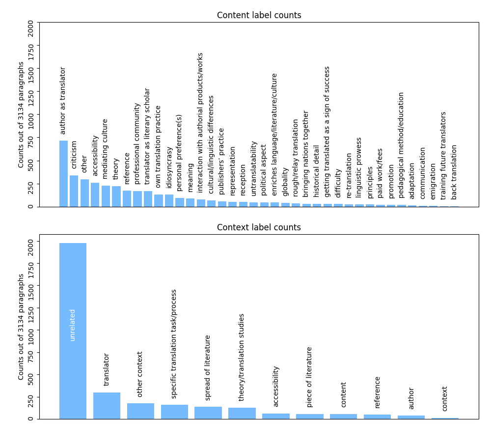
Figure 1: Train set label counts. The first context label refers to paragraphs that contain the subword “fordí” but are unrelated to translation.

2.4.5 Pruning and truncating paragraphs from Nagyvilág for the predict set

As for forming the predict set from the preprocessed Nagyvilág corpus, out of its 322,970 paragraphs, we selected the 12,712 that contained "fordí" as a subword. The dataset was further filtered by discarding (i) tables of contents, (ii) references at the end of quotations or literary texts that only consist of “translation by <translator>” and (iii) literary texts. This way, we ended up with a predict set of 4589 sequences. We truncated the tokenized sequences at 512 tokens in front.

3 Training

3.1 Pretraining: Domain adaptation

We started training with Masked Language Modelling on the 21,242,121-word Alföld–Nagyvilág dataset described in Subsection 2.4. The batch size to the largest value that fit in the NVIDIA A100 40GB GPU that we were using, and following Ma and Yarats [21], the number of warmup steps was set to $\frac{2}{1-\beta_{2}}$ train steps, where $\beta_{2}$ denotes the second momentum in the AdamW optimizer [22]. To tune the rest of the hyperparameters, the BlendSearch algorithm [23] was used. Training with the best hyperparameters that had been found brought down the perplexity score of 43.07 of the original PULI-BERT-Large model to 2.88.

3.2 Finetuning: Unbalanced label classification

As described in Subsection 2.4, we worked with a 3134-sequence finetuning train set with two highly unbalanced label sets: 38 content labels that are multilabel, and 12 context labels that are single label.

3.2.1 10-fold training and evaluation

The small size of the train set was taken advantage of by using techniques requiring several train runs. One of these is 10-fold training. Its benefits, incidentally, are 3-fold:

1. Consistency of evaluation scores across iterations confirm consistency of annotation.

2. More robust evaluation scores can be achieved with confidence intervals.

3. The 10 models acquired from training can be used for inference as an ensemble.

See Subsection 2.4 on how we procured an approximately stratified 10-fold partition for the content labels, that is the multilabel set.

3.2.2 Population-Based Training

The other technique with several runs we used is the application of Population-Based Training [24] for hyperparameter optimization. Its benefits are 2-fold:

1. It adapts hyperparameters on the fly and thus finds hyperparameter schedules on its own.

2. Since it trains the samples in parallel, it is highly scalable.

We ran this with population size 100 for 30 epochs for the content labels, and at least 30 epochs until there was no improvement for 10 epochs for the context labels. In our version of selection:

1. the top 10% elite is kept unchanged, and

2. roulette wheel selection is used for the rest with hyperparameter perturbation.

In contrast to Jaderberg et al. [24], in perturbation, we do not choose between the multipliers 0.8 and 1.2, but pick a multiplier uniformly from the interval $[0.8,1.2]$.

3.2.3 Content label finetuning

As the ultimate aim of the model was to detect trends in the perception of translation, and to this end to predict label counts for sections of the Nagyvilág corpus: months, years and decades of volumes, our plan was to sum the prediction probabilities for paragraphs in these time periods. In the content label, that is the multilabel case we could use ROC AUC as evaluation metric to focus more on evaluating whether the model gives positive cases higher probabilities than negative ones instead of just the predicted labels themselves (and thereby requiring to fix a threshold; more on this in Subsubsection 4.2.1). Furthermore, this metric is robust with respect to label unbalance.

To account even more for label unbalance, we used focal loss [25] as train loss. This gave a very satisfactory average ROC AUC of $0.9524\pm 0.0114$ (we report all of the confidence intervals with confidence level 95%). See more detailed evaluation results in Figure 2. Note that even less frequent labels do not get lower scores.

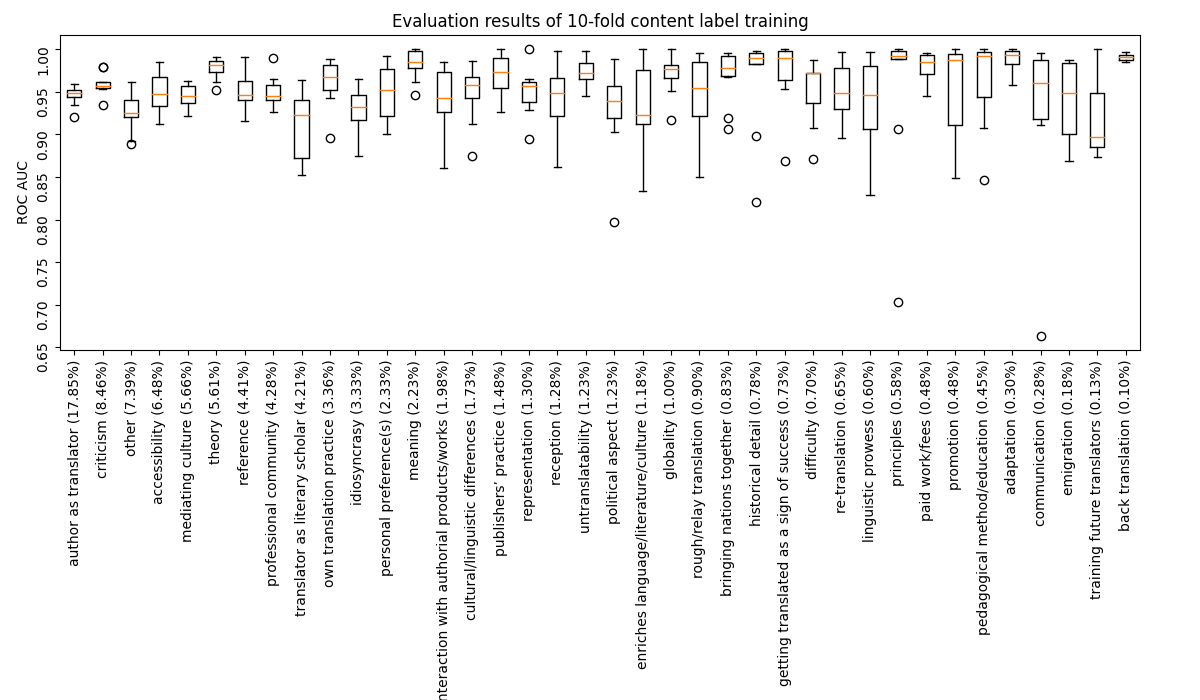
Figure 2: Evaluation results of 10-fold content label training. The percentages next to the label names indicate frequency.

3.2.4 Context label finetuning

In the context label, that is the multiclass single label case, we used balanced accuracy as evaluation metric. As training loss, we first used focal loss here also, but we were somewhat dissatisfied with the resulting balanced accuracy. Therefore, we combined label distribution-aware margin loss [26] with a penalty for confident output distributions [27]. This gave a better balanced accuracy of $0.6357\pm 0.1266$. See Figure 3 for more detailed evaluation results.

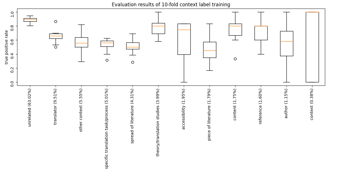
Figure 3: Evaluation results of 10-fold context label training. The percentages next to the label names indicate frequency.

Note that separate model ensembles were trained in the content and the context label case. We experimented with training combined models for the two label sets, but with significantly worse results.

3.3 Ablation studies

The training procedure was repeated with two alternatives. First, we ran the whole training pipeline with first pretraining as described in Subsection 3.1 and then finetuning as described in Subsection 3.2 using the earlier and smaller Hungarian LLM huBERT [28]. Then we tried running finetuning on the original PULI-BERT-Large model, that is with skipping domain adaptation. It turned out that both alternatives yielded less favourable results, see Table 1.

Table 1: Ablation studies

Model	Content label ROC AUC	Context label balanced accuracy
huBERT with domain adaptation	$0.9485\pm 0.0167$	$0.6173\pm 0.0872$
PULI-BERT-Large without domain adaptation	$0.9182\pm 0.0689$	$0.5545\pm 0.1422$
PULI-BERT-Large with domain adaptation	$\mathbf{0.9524\pm 0.0114}$	$\mathbf{0.6357\pm 0.1266}$

4 Inference

4.1 Validation on the predict set

4.1.1 Deciding the size of the validation set

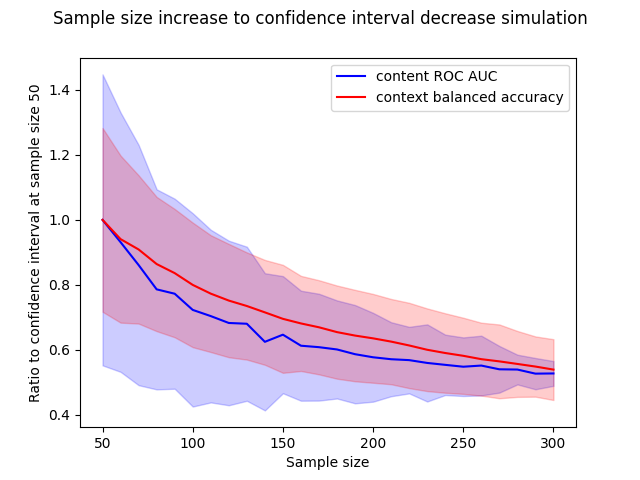
Figure 4: Sample size increase to confidence interval decrease simulation via bootstrap.

As manual validation is highly resource-intensive, when deciding on how many samples we should draw for the validation set, for a prospective sample size, we seeked to estimate what confidence interval is to be expected. To that end, simulations were run on the results of the 10-fold training: for both content and context labels, $\mathtt{sample\_size}=50,60,\ldots,300$ and each fold evaluation set, 100 times, we drew a random sample of sample_size from the fold evaluation set, and via bootstrapping with size 10,000 the standard deviation of the relevant metric was approximated, see Figure 4. This we could use to estimate what confidence interval we would get from what sample size. Based on this data, it was confirmed that going from 50 samples to 100 for a confidence interval decrease of about 20% is worthwhile, however, going up to 150 for a further confidence interval decrease of about 10% is not. Therefore a decision was made to draw 100 samples from the Nagyvilág predict set for manual validation.

4.1.2 Importance sampling on the predict set

As we naturally did not have labels for the predict set, only model prediction probabilities, a stratified sample for validation could not be used. Therefore, to address label unbalance, we opted for the following importance sampling approach, that draws paragraphs with less frequent label prediction probabilities with higher probability:

For $i=1,\ldots,5489$ and $\ell=1,\ldots,50$, let $p_{i,\ell}$ denote the average prediction probability for the $\ell$-th label (content or context) of the model ensemble on the $i$-th paragraph of the predict set. For each label index $\ell$, let $p_{\ell}=\max_{i=1}^{5489}p_{i,\ell}$ denote the maximum probability it received on the predict set. We split the intervals $[0,p_{\ell}]$ to five bins $I_{\ell,1}=[0,\frac{p_{\ell}}{5}),\ldots,I_{\ell,5}=[\frac{4p_{\ell}}{5},\ldots,p_{\ell}]$ of equal length. Then for each $j=1,\ldots,5$, we count for how many paragraphs the probabilities fall into the bin: $C_{\ell,j}=\#\{i=1,\ldots,5489:p_{i,\ell}\in I_{\ell}\}$. Finally, for a paragraph index $i$ and label index $\ell$, let $j_{i,\ell}$ denote the index of the bin the appropriate probability falls into: $p_{i,\ell}\in I_{j_{i,\ell}}$. With all of this, the sampling weight of the $i$-th paragraph is

$$w_{i}=\sum_{\ell=1}^{50}\frac{1}{C_{\ell,j_{i,\ell}}}.$$

4.1.3 Validation results

On the content label set, we achieved a ROC AUC of $0.8735\pm 0.0337$ (to get confidence intervals and box plots for the validation results, we used bootstrapping on 10,000 samples). For more detailed scores, see Figure 5. We were very pleased with this result as this meant that the model ensemble is capable of reliably carrying over the labeling to another domain.

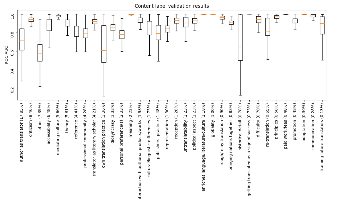
Figure 5: Content label validation results. The percentages next to the label names indicate frequency in the train set.

On the other hand, on the context label set, we only reached a balanced accuracy of $0.2995\pm 0.1374$. For more detailed scores, see Figure 6. We think that this could be attributed to the truncation described in Subsubsection 2.4.5, or the fact that context classification could require knowledge of surrounding paragraphs, which the architecture did not have. Based on this result, from Nagyvilág, only content labels were used in the findings.

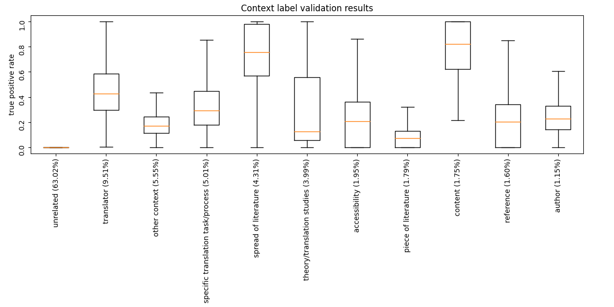
Figure 6: Context label validation results. The percentages next to the label names indicate frequency in the train set.

4.2 Postprocessing for analysis

4.2.1 Calibration by prediction probability truncation

It was time to transform the predictions to a form amenable for analysis. It was decided that instead of counting paragraphs with prediction probabilities $>50\%$, as is usually done for binary classification, the prediction probabilities themselves would be added up for better results.

First, the prediction probabilities needed to be calibrated. Although training with focal loss yields well calibrated models [29] and indeed, the estimated expected calibration error apparently could not be improved by a performant method such as beta calibration [30], summing up small nonzero probabilities still yielded unreasonable large predicted label counts. Therefore, we decided to use the following calibration method specifically tailored to this problem:

We decided to truncate the probabilities: if a probability $p$ is less than a threshold $p_{\mathrm{low}}$, then we set it to 0. To restore balance, if a probability $p$ is greater than another threshold $p_{\mathrm{high}}$, then we set it to 1. Grid search was run to find the thresholds $p_{\mathrm{low}}$ and $p_{\mathrm{high}}$: the metric is

$$\frac{1}{N}\sum_{\ell=1}^{N}\frac{|\sum_{i=1}^{M}p_{i,\ell}-\sum_{i=1}^{M}y_{i,\ell}|}{\sum_{i=1}^{M}y_{i,\ell}},$$

where $N=38$ is the number of content labels, $M=3134$ is the number of paragraphs in the train set, $p_{i,\ell}$ is the prediction probability of the $\ell$-th label on the $i$-th paragraph by the model out of 10 that has not been trained on the $i$-th paragraph, and $y_{i,\ell}\in\{0,1\}$ depending on whether the $\ell$-th label is on the $i$-th paragraph in the manual annotation.

In turned out that the best values are $p_{\mathrm{low}}=0.2$ and $p_{\mathrm{high}}=0.54$, with which we get an error rate of $11.61\%$. See Table 2 for more detailed results. We also checked that setting $p\leq 50\%$ to 0 and $p>50\%$ to 1, as is usually done in binary classification, gives the much higher error rate of $69.05\%$.

Table 2: Label count error rates in the train set

	Label count error rates
Label indices in decreasing order by frequency	No truncation	Setting probabilities $p<p_{\mathrm{low}}=0.2$ to 0	Setting probabilities $p<p_{\mathrm{low}}=0.2$ to 0 and $p>p_{\mathrm{high}}=0.54$ to 1
1–9	428.64%	14.41%	10.40%
10–19	267.22%	14.57%	10.27%
20–29	338.99%	18.43%	17.03%
30–38	640.15%	13.19%	8.51%
1–38 (cumulated)	418.22%	15.19%	11.61%

To measure if the model can correctly detect tendencies, as the train set was inadequate in size for this purpose, we used the following discretized method: let $\ell$ be a label index and let $y$ be a year. With this, let the $C_{\ell}$ denote a total label count (predicted or true) and $C_{\ell}(y)$ a yearly label count. Then we let a label tick be $t_{\ell}=\max(\frac{C_{\ell}}{40},1)$. Finally, for a year $y=1980,\ldots,1998$, the tendency value expresses if in two consecutive years the label counts have increased or decreased by at least a label tick:

$$T_{y}=\begin{cases}1&C_{\ell}(y+1)-C_{\ell}(y)\geq t_{\ell}\\ -1&C_{\ell}(y+1)-C_{\ell}(y)\leq-t_{\ell}\\ 0&\text{else}\end{cases}$$

We averaged the absolute tendency value differences of the predicted label counts from the ones in the annotation. Here too we found that the same calibration helps, see Table 3. The same $p_{\mathrm{low}}$ and $p_{\mathrm{high}}$ did not give the optimal results, but we decided to keep them for consistency and because for less data per year we trusted this second benchmark less.

Table 3: Label tendency error rates in the train set

	Label tendency error rates
Label indices in decreasing order by frequency	No truncation	Setting probabilities $p<p_{\mathrm{low}}=0.2$ to 0	Setting probabilities $p<p_{\mathrm{low}}=0.2$ to 0 and $p>p_{\mathrm{high}}=0.54$ to 1
1–9	29.24%	22.81%	27.49%
10–19	64.74%	44.21%	42.11%
20–29	58.95%	32.11%	40.00%
30–38	64.33%	17.54%	16.37%
1–38 (cumulated)	54.71%	29.64%	31.99%

4.2.2 Label relation networks

It was a primary goal of this project to analyze the relations and relational changes of the labels. To this end, we introduced label relation networks: these are directed weighted complete networks where the nodes are labels, and for two labels $\ell_{1},\,\ell_{2}$, the weight of the edge $\ell_{1}\to\ell_{2}$ is the conditional probability $\mathbf{P}(\ell_{2}|\ell_{1})$ as estimated by the manual annotations on Alföld or the model ensemble predictions on Nagyvilág or both.

To get the most useful representations for qualitative analysis, we used the Kamada–Kawai algorithm [31] as implemented in NetworkX [32] to determine the node layout, and then the network was drawn using PyGraphviz [33] in such a way that edge width indicates conditional probability. See Figure 7 for the full content label relation network based on the predicted probabilities on Nagyvilág.

The analysis of the data is discussed in Galambos [1].

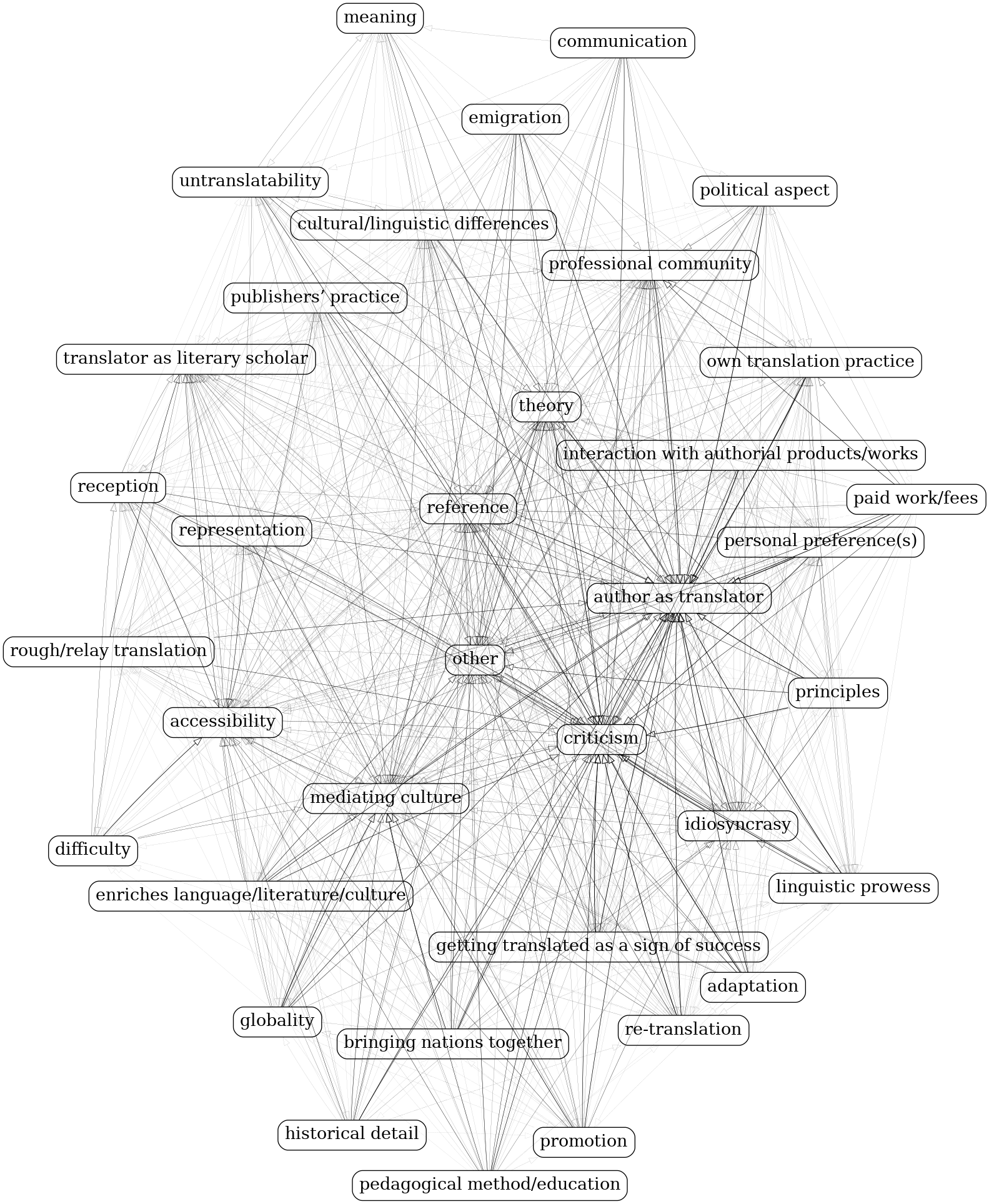
Figure 7: The full content label relation network based on the predicted probabilities on Nagyvilág

References

- Galambos [2023] Dalma Galambos. A műfordítás magyar képe (1980–2000). PhD thesis, Pázmány Péter Catholic University, 2023. Submitted for review.
- Vaswani et al. [2017] Ashish Vaswani, Noam Shazeer, Niki Parmar, Jakob Uszkoreit, Llion Jones, Aidan N. Gomez, Łukasz Kaiser, and Illia Polosukhin. Attention is all you need. In Proceedings of the 31st International Conference on Neural Information Processing Systems, NIPS’17, page 6000–6010, Red Hook, NY, USA, 2017. Curran Associates Inc. ISBN 9781510860964.
- Devlin et al. [2019] Jacob Devlin, Ming-Wei Chang, Kenton Lee, and Kristina Toutanova. BERT: Pre-training of deep bidirectional transformers for language understanding. In Proceedings of the 2019 Conference of the North American Chapter of the Association for Computational Linguistics: Human Language Technologies, Volume 1 (Long and Short Papers), pages 4171–4186, Minneapolis, Minnesota, June 2019. Association for Computational Linguistics. doi:10.18653/v1/N19-1423. URL https://aclanthology.org/N19-1423.
- Ring et al. [2020] Orsolya Ring, Zoltán Kmetty, Martina Katalin Szabó, László Kiss, Balázs Nagy, and Veronika Vincze. Kulcsfogalmak jelentésváltozása a kádár-korszak politikai diskurzusában. In Magyar Számítógépes Nyelvészeti Konferencia, pages 333–342, 2020. ISBN 978-963-306-719-2. URL http://acta.bibl.u-szeged.hu/67659/.
- Szabó et al. [2021] Martina Katalin Szabó, Orsolya Ring, Balázs Nagy, László Kiss, Júlia Koltai, Gábor Berend, László Vidács, Attila Gulyás, and Zoltán Kmetty. Exploring the dynamic changes of key concepts of the hungarian socialist era with natural language processing methods. Historical Methods: A Journal of Quantitative and Interdisciplinary History, 54(1):1–13, 2021. doi:10.1080/01615440.2020.1823289. URL https://doi.org/10.1080/01615440.2020.1823289.
- Bressem et al. [2020] Keno K Bressem, Lisa C Adams, Robert A Gaudin, Daniel Tröltzsch, Bernd Hamm, Marcus R Makowski, Chan-Yong Schüle, Janis L Vahldiek, and Stefan M Niehues. Highly accurate classification of chest radiographic reports using a deep learning natural language model pre-trained on 3.8 million text reports. Bioinformatics, 36(21):5255–5261, 07 2020. ISSN 1367-4803. doi:10.1093/bioinformatics/btaa668. URL https://doi.org/10.1093/bioinformatics/btaa668.
- Grandeit et al. [2020] Philipp Grandeit, Carolyn Haberkern, Maximiliane Lang, Jens Albrecht, and Robert Lehmann. Using BERT for qualitative content analysis in psychosocial online counseling. In Proceedings of the Fourth Workshop on Natural Language Processing and Computational Social Science, pages 11–23, Online, November 2020. Association for Computational Linguistics. doi:10.18653/v1/2020.nlpcss-1.2. URL https://aclanthology.org/2020.nlpcss-1.2.
- Limsopatham [2021] Nut Limsopatham. Effectively leveraging BERT for legal document classification. In Proceedings of the Natural Legal Language Processing Workshop 2021, pages 210–216, Punta Cana, Dominican Republic, November 2021. Association for Computational Linguistics. doi:10.18653/v1/2021.nllp-1.22. URL https://aclanthology.org/2021.nllp-1.22.
- Beltagy et al. [2020] Iz Beltagy, Matthew E. Peters, and Arman Cohan. Longformer: The long-document transformer. arXiv:2004.05150, 2020.
- Mehta et al. [2022] Maitrey Mehta, Derek Caperton, Katherine Axford, Lauren Weitzman, David Atkins, Vivek Srikumar, and Zac Imel. Psychotherapy is not one thing: Simultaneous modeling of different therapeutic approaches. In Proceedings of the Eighth Workshop on Computational Linguistics and Clinical Psychology, pages 47–58, Seattle, USA, July 2022. Association for Computational Linguistics. doi:10.18653/v1/2022.clpsych-1.5. URL https://aclanthology.org/2022.clpsych-1.5.
- Lacoste et al. [2019] Alexandre Lacoste, Alexandra Luccioni, Victor Schmidt, and Thomas Dandres. Quantifying the carbon emissions of machine learning. arXiv:1910.09700, 2019.
- in Data [2019] Our World in Data. Carbon footprint of travel per kilometer, 2019. https://ourworldindata.org/grapher/carbon-footprint-travel-mode, Last accessed on 2023-08-06.
- Braun and Clarke [2022] Virginia Braun and Victoria Clarke. Thematic Analysis: a practical guide. SAGE, London; Thousand Oaks, California, 2022.
- Magyarország [2023] Arcanum Adatbázis Kiadó Magyarország. Arcanum digitális tudománytár, 2023. https://adtplus.arcanum.hu/, Last accessed on 2023-07-31.
- The Tesseract Authors [2023] The Tesseract Authors. Tesseract, 2023. https://github.com/tesseract-ocr/tesseract, Last accessed on 2023-07-31.
- The Python Tesseract Authors [2022] The Python Tesseract Authors. Python tesseract, 2022. https://github.com/madmaze/pytesseract, Last accessed on 2023-07-31.
- Ester et al. [1996] Martin Ester, Hans-Peter Kriegel, Jörg Sander, and Xiaowei Xu. A density-based algorithm for discovering clusters in large spatial databases with noise. KDD’96, page 226–231. AAAI Press, 1996.
- Pedregosa et al. [2011] F. Pedregosa, G. Varoquaux, A. Gramfort, V. Michel, B. Thirion, O. Grisel, M. Blondel, P. Prettenhofer, R. Weiss, V. Dubourg, J. Vanderplas, A. Passos, D. Cournapeau, M. Brucher, M. Perrot, and E. Duchesnay. Scikit-learn: Machine learning in Python. Journal of Machine Learning Research, 12:2825–2830, 2011.
- Yang et al. [2023] Zijian Győző Yang, Réka Dodé, Gergő Ferenczi, Enikő Héja, Kinga Jelencsik-Mátyus, Ádám Kőrös, László János Laki, Noémi Ligeti-Nagy, Noémi Vadász, and Tamás Váradi. Jönnek a nagyok! bert-large, gpt-2 és gpt-3 nyelvmodellek magyar nyelvre. In XIX. Magyar Számítógépes Nyelvészeti Konferencia (MSZNY 2023), pages 247–262, Szeged, Hungary, 2023. Szegedi Tudományegyetem, Informatikai Intézet.
- Wolf et al. [2020] Thomas Wolf, Lysandre Debut, Victor Sanh, Julien Chaumond, Clement Delangue, Anthony Moi, Pierric Cistac, Tim Rault, Remi Louf, Morgan Funtowicz, Joe Davison, Sam Shleifer, Patrick von Platen, Clara Ma, Yacine Jernite, Julien Plu, Canwen Xu, Teven Le Scao, Sylvain Gugger, Mariama Drame, Quentin Lhoest, and Alexander Rush. Transformers: State-of-the-art natural language processing. In Proceedings of the 2020 Conference on Empirical Methods in Natural Language Processing: System Demonstrations, pages 38–45, Online, October 2020. Association for Computational Linguistics. doi:10.18653/v1/2020.emnlp-demos.6. URL https://aclanthology.org/2020.emnlp-demos.6.
- Ma and Yarats [2021] Jerry Ma and Denis Yarats. On the adequacy of untuned warmup for adaptive optimization. Proceedings of the AAAI Conference on Artificial Intelligence, 35(10):8828–8836, May 2021. doi:10.1609/aaai.v35i10.17069. URL https://ojs.aaai.org/index.php/AAAI/article/view/17069.
- Loshchilov and Hutter [2019] Ilya Loshchilov and Frank Hutter. Decoupled weight decay regularization. In 2019 International Conference on Learning Representations (ICLR), 2019. arXiv:1711.05101.
- Wang et al. [2021] Chi Wang, Qingyun Wu, Silu Huang, and Amin Saied. Economical hyperparameter optimization with blended search strategy. In ICLR, 2021.
- Jaderberg et al. [2017] Max Jaderberg, Valentin Dalibard, Simon Osindero, Wojciech M. Czarnecki, Jeff Donahue, Ali Razavi, Oriol Vinyals, Tim Green, Iain Dunning, Karen Simonyan, Chrisantha Fernando, and Koray Kavukcuoglu. Population based training of neural networks, 2017. URL https://arxiv.org/abs/1711.09846.
- Lin et al. [2017] Tsung-Yi Lin, Priya Goyal, Ross Girshick, Kaiming He, and Piotr Dollár. Focal loss for dense object detection. In 2017 IEEE International Conference on Computer Vision (ICCV), pages 2999–3007, 2017. doi:10.1109/ICCV.2017.324.
- Cao et al. [2019] Kaidi Cao, Colin Wei, Adrien Gaidon, Nikos Arechiga, and Tengyu Ma. Learning imbalanced datasets with label-distribution-aware margin loss. In Advances in Neural Information Processing Systems, pages 1567–1578, 2019.
- Pereyra et al. [2017] Gabriel Pereyra, George Tucker, Jan Chorowski, Łukasz Kaiser, and Geoffrey Hinton. Regularizing neural networks by penalizing confident output distributions. 2017. URL https://arxiv.org/abs/1701.06548.
- Nemeskey [2021] Dávid Márk Nemeskey. Introducing huBERT. In XVII. Magyar Számítógépes Nyelvészeti Konferencia (MSZNY2021), pages 3–14, Szeged, 2021. URL https://acta.bibl.u-szeged.hu/73353.
- Mukhoti et al. [2020] Jishnu Mukhoti, Viveka Kulharia, Amartya Sanyal, Stuart Golodetz, Philip Torr, and Puneet Dokania. Calibrating deep neural networks using focal loss. In H. Larochelle, M. Ranzato, R. Hadsell, M.F. Balcan, and H. Lin, editors, Advances in Neural Information Processing Systems, volume 33, pages 15288–15299. Curran Associates, Inc., 2020. URL https://proceedings.neurips.cc/paper_files/paper/2020/file/aeb7b30ef1d024a76f21a1d40e30c302-Paper.pdf.
- Kull et al. [2017] Meelis Kull, Telmo Silva Filho, and Peter Flach. Beta calibration: a well-founded and easily implemented improvement on logistic calibration for binary classifiers. In Aarti Singh and Jerry Zhu, editors, Proceedings of the 20th International Conference on Artificial Intelligence and Statistics, volume 54 of Proceedings of Machine Learning Research, pages 623–631. PMLR, 20–22 Apr 2017. URL https://proceedings.mlr.press/v54/kull17a.html.
- Kamada and Kawai [1989] Tomihisa Kamada and Satoru Kawai. An algorithm for drawing general undirected graphs. Information Processing Letters, 31(1):7–15, 1989. ISSN 0020-0190. doi:https://doi.org/10.1016/0020-0190(89)90102-6. URL https://www.sciencedirect.com/science/article/pii/0020019089901026.
- Hagberg et al. [2008] Aric A. Hagberg, Daniel A. Schult, and Pieter J. Swart. Exploring network structure, dynamics, and function using networkx. In Gaël Varoquaux, Travis Vaught, and Jarrod Millman, editors, Proceedings of the 7th Python in Science Conference, pages 11 – 15, Pasadena, CA USA, 2008.
- The PyGraphviz Authors [2022] The PyGraphviz Authors. Pygraphviz, 2022. https://github.com/pygraphviz/pygraphviz, Last accessed on 2023-08-04.