Phase transitions in self-gravitating systems and bacterial populations
surrounding a central body

Abstract

We study the nature of phase transitions in a self-gravitating classical gas in the presence of a central body. The central body can mimic a black hole at the center of a galaxy or a rocky core (protoplanet) in the context of planetary formation. In the chemotaxis of bacterial populations, sharing formal analogies with self-gravitating systems, the central body can be a supply of “food” (chemoattractant). We consider both microcanonical (fixed energy) and canonical (fixed temperature) descriptions and study the inequivalence of statistical ensembles. At high energies (resp. high temperatures), the system is in a “gaseous” phase and at low energies (resp. low temperatures) it is in a condensed phase with a “cusp-halo” structure, where the cusp corresponds to the rapid increase of the density of the gas at the contact with the central body. For a fixed density $\rho_{*}$ of the central body, we show the existence of two critical points in the phase diagram, one in each ensemble, depending on the core radius $R_{*}$: for small radii $R_{*}<R_{*}^{\rm MCP}$, there exist both microcanonical and canonical phase transitions (that are zeroth and first order); for intermediate radii $R_{*}^{\rm MCP}<R_{*}<R_{*}^{\rm CCP}$, only canonical phase transitions are present; and for large radii $R_{*}>R_{*}^{\rm CCP}$, there is no phase transition at all. We study how the nature of these phase transitions changes as a function of the dimension of space. We also discuss the analogies and the differences with phase transitions in the self-gravitating Fermi gas [P. H. Chavanis, Phys. Rev. E 65, 056123 (2002)].

I Introduction

Self-gravitating systems have a very peculiar thermodynamics due to the unshielded long-range attractive nature of the gravitational interaction paddy ; dvs1 ; dvs2 ; katzrevue ; ijmpb . Their study is interesting both from the viewpoint of astrophysics and statistical mechanics since a collection of $N$ stars (composing globular clusters, galaxies…) constitutes a fundamental physical system with long-range interactions houches ; cdr ; campabook . The subject started with the seminal paper of Antonov antonov who considered the thermodynamics of a self-gravitating classical gas confined within a spherical box of radius $R$. Since the system is isolated, it must be studied in the microcanonical ensemble. The box is necessary to prevent the evaporation of the gas and make the problem well-posed mathematically. Following Ogorodnikov ogo1 ; ogo2 , Antonov studied the problem of maximizing the Boltzmann entropy at fixed mass and energy, and discovered that there is no global entropy maximum. There is not even an extremum of entropy (canceling the first order variations of entropy at fixed mass and energy) if the energy is below a critical value $E_{c}=-0.335GM^{2}/R$ antonov . Lynden-Bell and Wood lbw (see also Lynden-Bell lb ) interpreted this mathematical result in terms of a gravitational collapse that they called gravothermal catastrophe. Below the Antonov threshold $E<E_{c}$, the system takes a “core-halo” structure. The core, which has a negative specific heat, becomes hotter as it loses energy to the profit of the halo. Therefore, it continues to lose energy and evolves away from equilibrium. By this process, the system becomes hotter and hotter and more and more centrally condensed (as a consequence of the virial theorem). From thermodynamical arguments, the end-product of the gravothermal catastrophe is expected to be a binary star having a small mass ($2m\ll M$) but a huge binding energy henonbinary . The potential energy released by the binary star is redistributed in the halo in the form of kinetic energy (the system heats up) leading to an infinite (very large) entropy. Cohn cohn studied the dynamical evolution of the gravothermal catastrophe in the microcanonical ensemble (fixed energy) by numerically solving the orbit-averaged-Fokker-Planck equation. He found that the collapse is self-similar and that the density profile develops a finite time singularity (core collapse). The central density becomes infinite in a finite time, scaling as $\rho\sim r^{-2.23}$, but the core mass $M_{0}(t)\sim(t_{\rm coll}-t)^{0.41}$ tends to zero at the collapse time. Therefore, the divergence of the central density is simply due to a few stars approaching each other. In fact, a binary star is formed in the post-collapse regime and releases so much energy that the halo re-expands in a self-similar manner inagakilb . Finally, a series of gravothermal oscillations follows sugimoto . On the other hand, at sufficiently high energies $E>E_{c}$, there exist statistical equilibrium states in the form of local entropy maxima at fixed mass and energy (there may also be saddle points of entropy but they are unstable) antonov . These states are metastable but they are very long lived because their lifetime scales like $e^{N}$ (with $N\sim 10^{6}$ in a globular cluster) lifetime . Therefore, these gaseous states can play an important role in the dynamics bt . Indeed, most stellar systems like globular clusters are in the form of metastable gaseous states. They are described by the Michie-King model michie ; king which is a truncated Boltzmann distribution taking into account the evaporation of high energy stars. The thermodynamics of tidally truncated self-gravitating systems was studied by Katz katzking and Chavanis et al. clm1 . In practice, a globular cluster relaxes through gravitational encounters towards a truncated equilibrium state. As it slowly evaporates, its central density increases (as a consequence of the virial theorem) and the cluster follows the King sequence with higher and higher central densities until a point at which is becomes unstable and undergoes core collapse as described above.

Since the statistical ensembles are not equivalent for self-gravitating systems (see thirring ; lblb for early works on the subject and paddy ; dvs1 ; dvs2 ; katzrevue ; ijmpb for reviews), it can be of interest to study what happens when the system is in contact with a thermal bath imposing the temperature. In that case, the evolution of the system is dissipative and it must be studied in the canonical ensemble (CE). If one considers the problem of minimizing the free energy at fixed mass, one finds that there is no global minimum of free energy. There is not even an extremum of free energy (canceling the first variations of free energy at fixed mass) below a critical temperature $T_{c}=GMm/2.52k_{B}R$ discovered by Emden emden . The absence of a minimum of free energy leads to an isothermal collapse aa1 . From statistical mechanics arguments, the end-product of this gravitational collapse is expected to be a Dirac peak containing all the mass since this structure has an infinite free energy. This has actually be proven rigorously by Kiessling kiessling . Chavanis et al. crs ; sc studied the dynamical evolution of the isothermal collapse for $T<T_{c}$ in the canonical ensemble (fixed temperature) by solving numerically and analytically the Smoluchowski-Poisson system describing a gas of self-gravitating Brownian particles in an overdamped limit. They found that the pre-collapse is self-similar and that the density profile develops a finite time singularity. The central density becomes infinite in a finite time, scaling as $\rho\sim r^{-2}$, but the core mass $M_{0}(t)\sim(t_{\rm coll}-t)^{1/2}$ tends to zero at the collapse time. Therefore, “the central singularity contains no mass” in apparent contradiction with the thermodynamical expectation. In fact, the collapse continues after the singularity and a Dirac peak containing all the mass is finally formed in the post-collapse regime post . On the other hand, at sufficiently high temperatures $T>T_{c}$, there exist statistical equilibrium states in the form of local free energy minima at fixed mass (there may also be saddle points of free energy but they are unstable) aa1 . These states are metastable but they are very long lived since their lifetime scales like $e^{N}$ lifetime . Therefore, these gaseous states can, again, play an important role in the dynamics. The self-gravitating Brownian gas may describe the evolution of planetesimals in the solar nebula in the context of planet formation. In that case, the particles experience a friction with the gas and a stochastic force due to Brownian motion or turbulence aaplanetes . If the gas of particles is sufficiently dense (e.g., at special locations such as large-scale vortices), self-gravity becomes important leading to gravitational collapse and planet formation.

The caloric curve of classical self-gravitating systems has the form of a spiral and the stability of the equilibrium states can be determined by using the Poincaré turning point criterion poincare ; lbw ; katzpoincare1 . It is then found that the equilibrium states in the canonical ensemble become unstable after the first turning point of temperature $T_{c}$ (corresponding to a density contrast of $32.1$) while the equilibrium states in the microcanonical ensemble become unstable later, after the first turning point of energy (corresponding to a density contrast of $709$). Therefore, the statistical ensembles are inequivalent lbw ; thirring ; lblb , which is a fundamental feature of systems with long-range interactions campabook . For classical self-gravitating systems, the region of ensemble inequivalence corresponds to a region of negative specific heats which is allowed (stable) in the microcanonical ensemble but forbidden (unstable) in the canonical ensemble.

Since the core collapse of classical point masses leads to a singularity (a binary star in the microcanonical ensemble or a Dirac peak in the canonical ensemble), some authors have studied what happens when a physical short-range regularization is introduced in the problem. In that case, we expect a phase transition between a gaseous (dilute) phase which is independent of the small-scale regularization and a condensed phase in which the small-scale regularization plays a prevalent role. Aronson and Hansen aronson considered the case of a self-gravitating hard-sphere gas in the canonical ensemble, modeled by a van der Waals equation of state, and evidenced a first order canonical phase transition when the filling factor $\mu=R/R_{*}$ (where $R$ is the system size and $R_{*}\sim N^{1/3}a$ is the radius of a compact object in which all the particles of size $a$ are packed together) is sufficiently large. In the condensed phase, the equilibrium state has a “core-halo” structure with a dense solid core surrounded by a dilute atmosphere. Their study was followed by Stahl et al. stahl who used a more accurate equation of state and discussed interesting applications to planet formation. These authors considered both canonical and microcanonical ensembles and evidenced a first order microcanonical phase transition in the case of very large filling factors. Instead of considering a classical hard-sphere gas, one can also consider a gas of self-gravitating fermions described by the Fermi-Dirac statistics. This system can have application in the context of white dwarf stars chandrab , neutron stars ov ; shapiroteukolsky , and dark matter halos made of massive neutrinos bmtv ; btv ; vss ; rar ; mg16F ; predictiveF ; arguellerevue . In that case, the Pauli exclusion principle creates an “effective” repulsion between the particles and plays a role similar to that played by the core radius of classical particles in a hard sphere gas. For self-gravitating fermions, the end-product of the collapse is a “core-halo” structure with a degenerate core (equivalent to a polytrope of index $n=3/2$) surrounded by a dilute atmosphere. In the context of dark matter halos, the quantum core is called a “fermion ball”. The statistical mechanics of self-gravitating fermions was first considered by Hertel and Thirring htf who showed rigorously (in a mathematical sense) that the mean field approximation is exact in a proper thermodynamic limit. In another paper, Hertel and Thirring ht2 , and later Bilic and Viollier bvNR , discussed first order canonical phase transitions in the self-gravitating Fermi gas but did not evidence first order microcanonical phase transitions in their study. Chavanis ptfermi performed an exhaustive study of phase transitions in the self-gravitating Fermi gas in both canonical and microcanonical ensembles and explored the whole range of parameters. He showed the existence of two critical points, one in each ensemble. The control parameter can be written as $\mu=17.2587(R/R_{*})^{3/2}$, where $R$ is the system size and $R_{*}=0.181433\,h^{2}/(Gm^{8/3}g^{2/3}M^{1/3})$ is the radius of a completely degenerate object of mass $M$ at $T=0$ (“white dwarf”) determined by the Planck constant $\hbar$ ijmpb . Since $R_{*}$ is fixed by quantum mechanics (for a given mass $M$), the control parameter measures the size of the system $R$. For large systems ($\mu>\mu_{\rm MCP}\simeq 2670$), there exist both microcanonical and canonical phase transitions (of zeroth and first order), for systems of intermediate size ($\mu_{\rm CCP}<\mu<\mu_{\rm MCP}$) only canonical phase transitions exist, and for small systems ($\mu<\mu_{\rm CCP}\simeq 83$) there is no phase transition at all. Other types of small-scale regularization have been introduced and lead to a similar phenomenology my ; fl ; ym ; ci ; dv . A review of phase transitions in self-gravitating systems is given in ijmpb . These results have been extended to self-gravitating fermions in general relativity bvR ; rc ; calettre ; acepjb . They have also been discussed in the context of the fermionic King model (avoiding the artificial box) in Newtonian gravity clm2 and general relativity adky .

In the present work, we study the nature of phase transitions in a self-gravitating classical gas of point-like particles in the presence of a central body. The central body could mimic the effect of a black hole at the center of a galaxy or at the center of a globular cluster. It could also represent a rocky core (protoplanet) at the center of a giant gaseous planet like Jupiter or Saturn. The central body prevents the formation of singularities resulting from gravitational collapse and plays a role similar to that of a short-range regularization. There exists an equilibrium state for all accessible values of energy and temperature but canonical and microcanonical phase transitions can take place between a gaseous phase and a condensed phase. The condensed phase has the structure of a giant gaseous planet with a solid core surrounded by an atmosphere. The atmosphere has a “cusp-halo” structure, where the cusp corresponds to the rapid increase of the density of the gas at the contact with the central body. For a fixed density $\rho_{*}$ of the central body (and a fixed system size $R$), we show the existence of two critical points in the phase diagram, one in each ensemble, depending on the core radius $R_{*}$. For small radii $R_{*}<R_{*}^{\rm MCP}$, there exist both microcanonical and canonical phase transitions (that are zeroth and first order). For intermediate radii $R_{*}^{\rm MCP}<R_{*}<R_{*}^{\rm CCP}$, only canonical phase transitions are present. Finally, for large radii $R_{*}>R_{*}^{\rm CCP}$, there is no phase transition at all. This is qualitatively similar to the results previously obtained for self-gravitating fermions ijmpb . We also study how the canonical and microcanonical critical points $R_{*}^{\rm CCP}$ and $R_{*}^{\rm MCP}$ depend on the density of the central body $\rho_{*}$.

Our results can also have applications for the problem of chemotaxis in biology murray . Indeed, there exists a remarkable analogy between self-gravitating systems and bacterial populations crrs . In this analogy, the density of the gas $\rho({\bf r},t)$ is the counterpart of the density of bacteria $\rho({\bf r},t)$, and minus the gravitational potential $-\Phi({\bf r},t)$ is the counterpart of the concentration $c({\bf r},t)$ of the chemical (“pheromone”) produced by the bacteria (see Appendix A). As a result, the counterpart of a central mass $M_{*}$ (black hole, protoplanet,…) giving rise to an external gravitational force $-\nabla\Phi_{\rm ext}$ is a supply of “food” (chemoattractant) giving rise to a chemical drift $\nabla c_{\rm ext}({\bf r})$. Therefore, our study can have applications in biology up to a straightforward change of notations.

In this article, we will use the notations of astrophysics in order to make the connection with previous studies. We will essentially consider the spatial dimension $d=3$ which is the most relevant dimension in astrophysics, and which leads to the richest variety of phase transitions. It corresponds to spherical halos and stars chandrab . However, the dimension $d=2$ corresponding to cosmic filaments stodolkiewicz ; ostriker and the dimension $d=1$ corresponding to sheets or pancakes spitzer ; camm have also been considered in astrophysics. On the other hand, the dimension $d=2$ is particularly relevant in biology chemo2d since cells of bacteria can be cultured on a petri dish. We will therefore study how the nature of phase transitions changes as a function of the dimension of space. A similar study of the effect of the dimension of space on the nature of gravitational phase transitions has been performed in sc for classical self-gravitating systems, in ptd ; wdd ; kmcfermions ; kmcbosons for self-gravitating fermions and bosons, and in exclusion ; bbkmm for particles with an exclusion constraint in position space.

The paper is organized as follows. In Sec. II we derive the basic equations determining the equilibrium structure of a self-gravitating isothermal gas around a central body. In Sec. III we plot the caloric curves of this self-gravitating gas in $d=3$ dimensions and study the corresponding phase transitions. In Sec. IV we briefly consider the case of the dimensions $d=1$ and $d=2$. The Appendices regroup useful formulae that are needed in the theoretical part of the paper.

II Equilibrium structure of a self-gravitating isothermal gas around a central body

II.1 The maximum entropy principle

We consider a system of $N$ point-like particles of mass $m$ interacting via Newtonian gravity in a space of dimension $d$. We allow for the presence of a spherically symmetric central body of mass $M_{*}$ and radius $R_{*}$. This central body may mimic a black hole at the center of a galaxy or at the center of a globular cluster. It may also describe a rocky core surrounded by a gas (atmosphere) in the context of planet formation. The particles are enclosed within a spherical box of radius $R$ so as to prevent the evaporation of the gas and make a statistical equilibrium state well-defined. Physically, a gas is never completely isolated from the surrounding. Therefore, the box can play the role of a tidal radius in the case of globular clusters and dark matter halos or represent the Hill sphere in the context of planet formation. The Hamiltonian of the self-gravitating system is

$$H=\sum_{i}\frac{1}{2}mv_{i}^{2}+m^{2}\sum_{i<j}u(|{\bf r}_{i}-{\bf r}_{j}|)+m\sum_{i}\Phi_{\rm ext}({\bf r}_{i}),$$ (1)

where $i=1,...,N$ runs over the particles of the gas. The first term is the kinetic energy, the second term represents the interaction energy of the particles of the gas and the third term takes into account the interaction between the gas and the central body. The gravitational potential of interaction in $d$ dimensions is given by

$$u(|{\bf r}-{\bf r}^{\prime}|)=-\frac{1}{d-2}\frac{G}{|{\bf r}-{\bf r}^{\prime}|^{d-2}}\qquad(d\neq 2),$$ (2)

$$u(|{\bf r}-{\bf r}^{\prime}|)=G\ln\frac{|{\bf r}-{\bf r}^{\prime}|}{R}\qquad(d=2).$$ (3)

We treat the influence of the central body as an external potential (see Appendix B):

$$\Phi_{\rm ext}({\bf r})=-\frac{1}{d-2}\frac{GM_{*}}{r^{d-2}}\quad(d\neq 2),$$ (4)

$$\Phi_{\rm ext}({\bf r})=GM_{*}\ln\left(\frac{r}{R}\right)\quad(d=2).$$ (5)

Let $f({\bf r},{\bf v})$ denote the distribution function of the system, i.e., $f({\bf r},{\bf v})d{\bf r}d{\bf v}$ gives the mass of the particles of the gas whose position and velocity are in the cell $({\bf r},{\bf v};{\bf r}+d{\bf r},{\bf v}+d{\bf v})$. The integral of $f$ over the velocity determines the spatial density $\rho=\int fd{\bf v}$. The total mass of the gas is

$$M=\int\rho\,d{\bf r}.$$ (6)

The spatial integral extends only in the region surrounding the central body, i.e., in the region $R_{*}<r<R$ covered by the gas. We consider a proper thermodynamic limit $N\rightarrow+\infty$ for self-gravitating systems in such a way that the rescaled energy and the rescaled temperature

$$\Lambda=-\frac{ER^{d-2}}{GM^{2}},\qquad\eta=\frac{\beta GMm}{R^{d-2}},$$ (7)

are independent on $N$. We also introduce the parameters

$$\mu=\frac{M_{*}}{M},\qquad\zeta=\frac{R_{*}}{R},$$ (8)

which represent the normalized mass and the normalized radius of the central body. In the $N\rightarrow+\infty$ limit, the mean field approximation is exact, except close to a critical point paddy ; dvs1 ; dvs2 ; katzrevue ; ijmpb ; houches ; cdr ; campabook . Therefore, ignoring the correlations between the particles of the gas, the total energy of the system can be expressed as

$$E=\frac{1}{2}\int fv^{2}\,d{\bf r}d{\bf v}+\frac{1}{2}\int\rho\Phi\,d{\bf r}+\int\rho\Phi_{\rm ext}\,d{\bf r},$$ (9)

where $\Phi_{\rm ext}({\bf r})$ is the potential created by the central body and $\Phi({\bf r})$ is the gravitational potential created by the gas (see Appendix B). For $R_{*}\leq r\leq R$, they are respectively the solutions of the Laplace equation

$$\Delta\Phi_{\rm ext}=0,$$ (10)

and the Poisson equation

$$\Delta\Phi=S_{d}G\rho,$$ (11)

where $S_{d}=2\pi^{d/2}/\Gamma(d/2)$ is the surface of a unit sphere in $d$ dimensions. The energy $E=E_{\rm kin}+W_{\rm tot}$ of the gas is the sum of its kinetic energy $E_{\rm kin}=(1/2)\int fv^{2}\,d{\bf r}d{\bf v}$ and its total potential energy $W_{\rm tot}=W+W_{\rm ext}$, where $W=(1/2)\int\rho\Phi\,d{\bf r}$ is the self-gravitating energy of the gas and $W_{\rm ext}=\int\rho\Phi_{\rm ext}\,d{\bf r}$ is the gravitational energy of the gas in the potential created by the central body (see Appendix B).

For isolated Hamiltonian systems, the mass and the energy are conserved and the thermodynamical potential is the Boltzmann entropy

$$S_{B}=-k_{B}\int\frac{f}{m}\ln\frac{f}{m}d{\bf r}d{\bf v}.$$ (12)

The Boltzmann entropy $S_{B}=k_{B}\ln{\cal W}$ measures the “disorder” of the system. It is proportional to the logarithm of the number ${\cal W}(\{n_{i}\})$ of microstates corresponding to a given macrostate ogorodnikov . At statistical equilibrium, the system is in the most mixed state consistent with all the constraints of the dynamics. Therefore, if the system is isolated, the equilibrium state maximizes the Boltzmann entropy $S_{B}$ at fixed mass $M$ and energy $E$ (microcanonical description). We thus have to solve the maximization problem

$$\max_{f}\quad\{S_{B}[f]\quad|\quad E[f]=E,\quad M[f]=M\}.$$ (13)

Alternatively, if the system is in contact with a heat bath imposing the temperature $T$, only the mass is conserved and the thermodynamical potential is the Boltzmann free energy $F_{B}=E-TS_{B}$. It is often more convenient to work with the Massieu function

$$J_{B}=\frac{S_{B}}{k_{B}}-\beta E,$$ (14)

where $\beta=1/(k_{B}T)$ is the inverse temperature. The Massieu function is the Legendre transform of the entropy with respect to the energy. If the system is in contact with a heat bath, the equilibrium state maximizes the Massieu function $J$ at fixed mass $M$ (canonical description). We thus have to solve the maximization problem

$$\max_{f}\quad\{J_{B}[f]\quad|\quad M[f]=M\}.$$ (15)

The microcanonical ensemble is the proper description for (isolated) Hamiltonian systems and the canonical ensemble is the proper description for (dissipative) Brownian systems ijmpb .

The extrema of entropy at fixed mass and energy (canceling the first order variations of entropy under constraints) are determined by the variational principle

$$\frac{\delta S_{B}}{k_{B}}-\beta\delta E-\alpha_{0}\delta M=0,$$ (16)

where $\beta$ and $\alpha_{0}$ are Lagrange multipliers associated with the conservation of $E$ and $M$. The extrema of Massieu function at fixed mass (canceling the first order variations of Massieu function under constraints) are determined by the variational principle

$$\delta J_{B}-\alpha_{0}\delta M=0,$$ (17)

where $\alpha_{0}$ is a Lagrange multiplier associated with the conservation of $M$. Using the identities

$$\delta S_{B}=-k_{B}\int\frac{\delta f}{m}\left(\ln\frac{f}{m}+1\right)\,d{\bf r}d{\bf v},$$ (18)

$$\delta E=\frac{1}{2}\int\delta fv^{2}\,d{\bf r}d{\bf v}+\int\Phi\delta\rho\,d{\bf r}+\int\Phi_{\rm ext}\delta\rho\,d{\bf r},$$ (19)

$$\delta M=\int\delta f\,d{\bf r}d{\bf v},$$ (20)

we find that the variational principles (16) and (17) lead to the mean field Maxwell-Boltzmann distribution

$$f=A^{\prime}e^{-\beta m[v^{2}/2+\Phi({\bf r})+\Phi_{\rm ext}({\bf r})]},$$ (21)

where $A^{\prime}=me^{-\alpha_{0}m-1}$. Introducing the local (kinetic) pressure $P({\bf r})=\frac{1}{d}\int fv^{2}\,d{\bf v}$ (see Appendix C), we find that the barotropic equation of state corresponding to the distribution (21) is that of an isothermal gas

$$P({\bf r})=\rho({\bf r})\frac{k_{B}T}{m}.$$ (22)

As a result, the velocity dispersion $\langle v^{2}\rangle=dP/\rho=dk_{B}T/m$ is constant. Integrating Eq. (21) over the velocity, we find that the spatial density is the mean field Boltzmann distribution

$$\rho=Ae^{-\beta m[\Phi({\bf r})+\Phi_{\rm ext}({\bf r})]},$$ (23)

where $A=(2\pi/\beta m)^{d/2}A^{\prime}$. Therefore, combining Eqs. (11) and (23), the structure of the gas around the central body is obtained by solving the Boltzmann-Poisson equation

$$\Delta\Phi=S_{d}GAe^{-\beta m(\Phi+\Phi_{\rm ext})}$$ (24)

with appropriate boundary conditions (see below), and by relating the Lagrange multipliers to the constraints. We can then plot the series of equilibria $\beta(E)$ for given values of $M_{*}$ and $R_{*}$ (or in dimensionless form $\eta(\Lambda)$ for given $\mu$ and $\zeta$). The control parameter is $E$ in the microcanonical ensemble and $\beta$ in the canonical ensemble. The stable region of the series of equilibria defines the caloric curve in the considered ensemble. Note that the extrema (regarding the first variations) of the entropy $S_{B}$ at fixed $E$ and $M$, and the extrema of the Massieu function $J_{B}$ at fixed $T$ and $M$ are the same, and both determine a self-gravitating isothermal gas. However, the stability of the gas (regarding the second variations of $S_{B}$ or $J_{B}$ with appropriate constraints) may differ in the microcanonical (fixed $E$) and canonical (fixed $T$) ensembles. When this happens, this is referred to a situation of ensemble inequivalence. It can be shown that canonical stability (Eq. (15)) implies microcanonical stability (Eq. (13)), but the converse is in general false for systems with long-range interactions ellis ; cc . For example, negative specific heats are forbidden in the canonical ensemble while they are allowed in the microcanonical ensemble. Therefore, canonical stability only provides a sufficient condition of microcanonical stability. Ensemble inequivalence and phase transitions in self-gravitating systems is well-documented in the absence of a central body paddy ; dvs1 ; dvs2 ; katzrevue ; ijmpb . We shall study how the presence of a central body affects these results.

II.2 The Emden equation

Introducing the total gravitational potential

$$\Phi_{\rm tot}=\Phi+\Phi_{\rm ext},$$ (25)

and using Eq. (10), we can rewrite the Boltzmann-Poisson equation (24) as

$$\Delta\Phi_{\rm tot}=S_{d}GAe^{-\beta m\Phi_{\rm tot}}.$$ (26)

It can be shown that the maximum entropy state of a non-rotating self-gravitating system is spherically symmetric antonov . In that case, we can rewrite the foregoing equation as

$$\frac{1}{r^{d-1}}\frac{d}{dr}\left(r^{d-1}\frac{d\Phi_{\rm tot}}{dr}\right)=S_{d}GAe^{-\beta m\Phi_{\rm tot}}.$$ (27)

It has to be solved with the boundary condition

$$\frac{d\Phi_{\rm tot}}{dr}(R_{*})=\frac{d\Phi_{\rm ext}}{dr}(R_{*})=\frac{GM_{*}}{R_{*}^{d-1}}$$ (28)

resulting from Eq. (97) and the fact that $d\Phi/dr(R_{*})=0$, since $\rho=0$, for $r\leq R_{*}$ (see Appendix D). Multiplying Eq. (27) by $r^{d-1}$, integrating between $R_{*}$ and $r$, and using the boundary condition (28), we obtain the integrodifferential equation

$$r^{d-1}\frac{d\Phi_{\rm tot}}{dr}=GM_{*}+GA\int_{R_{*}}^{r}e^{-\beta m\Phi_{\rm tot}(r^{\prime})}S_{d}\,{r^{\prime}}^{d-1}\,dr^{\prime}.$$ (29)

This equation can also be written as

$$\frac{d\Phi_{\rm tot}}{dr}=\frac{GM_{\rm tot}(r)}{r^{d-1}},$$ (30)

where

$$M_{\rm tot}(r)=M_{*}+M(r)=M_{*}+\int_{R_{*}}^{r}\rho(r^{\prime})S_{d}\,{r^{\prime}}^{d-1}\,dr^{\prime}$$ (31)

is the total mass contained within the sphere of radius $r$. This is Newton’s law in $d$ dimensions (see Appendix D).

To determine the structure of the isothermal gas, we introduce the function

$$\psi=\beta m(\Phi_{\rm tot}-\Phi_{\rm tot,0}),$$ (32)

where $\Phi_{\rm tot,0}=\Phi_{\rm tot}(R_{*})$ is the total gravitational potential at $r=R_{*}$. Then, the density can be written as

$$\rho=\rho_{0}e^{-\psi},$$ (33)

where $\rho_{0}=\rho(R_{*})$ is the density of the gas at the contact with the central body. By an abuse of language, $\rho_{0}$ will be called the central density and $\Phi_{\rm tot,0}$ will be called the central total gravitational potential. Introducing the dimensionless radius

$$\xi=(S_{d}G\beta m\rho_{0})^{1/2}r,$$ (34)

the Boltzmann-Poisson equation (27) reduces to the form

$$\frac{1}{\xi^{d-1}}\frac{d}{d\xi}\left(\xi^{d-1}\frac{d\psi}{d\xi}\right)=e^{-\psi},$$ (35)

which is called the Emden equation emden ; chandrab . In the presence of a central body, this equation has to be solved with the boundary conditions [see Eq. (28)]

$$\psi(\xi_{0})=0,\qquad\psi^{\prime}(\xi_{0})=\frac{\eta_{0}}{\xi_{0}},$$ (36)

where we have defined

$$\xi_{0}=(S_{d}G\beta m\rho_{0})^{1/2}R_{*},\qquad\eta_{0}=\beta GM_{*}m/R_{*}^{d-2}.$$ (37)

In the absence of a central body, the boundary conditions are replaced by $\psi(0)=\psi^{\prime}(0)=0$ emden ; chandrab . The Emden equation (35) can also be written in the form of an integrodifferential equation [see Eq. (29)]

$$\xi^{d-1}\frac{d\psi}{d\xi}=\eta_{0}\xi_{0}^{d-2}+\int_{\xi_{0}}^{\xi}e^{-\psi(\xi^{\prime})}{\xi^{\prime}}^{d-1}\,d\xi^{\prime}.$$ (38)

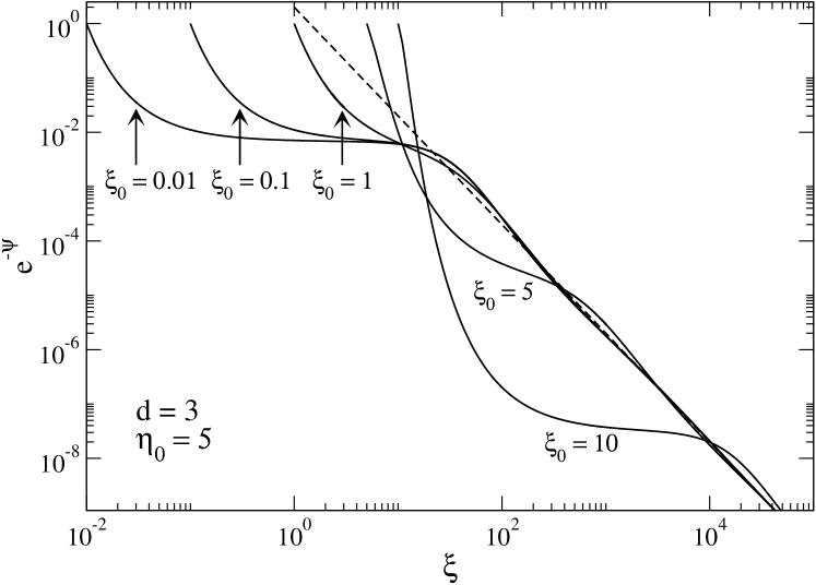
(a)    (b)

Figure 1: Dimensionless density profile $e^{-\psi}$ that is the solution of the Emden equation with a central body in $d=3$ dimensions. We have selected $\eta_{0}=5$ and $\eta_{0}=0$ (hole) for illustration.

The Emden equation (35) must be solved numerically (see Fig. 1). We can however easily determine the asymptotic behaviors of the solutions. For $\xi\rightarrow\xi_{0}$, we can expand the solution in Taylor series and we find that

$$\psi(\xi) = \frac{\eta_{0}}{\xi_{0}}\left(\xi-\xi_{0}\right)+\frac{1}{2}\left[1-\frac{(d-1)\eta_{0}}{\xi_{0}^{2}}\right]\left(\xi-\xi_{0}\right)^{2}$$

$$+\frac{1}{6}\left[\frac{1-d-\eta_{0}}{\xi_{0}}+\frac{d(d-1)\eta_{0}}{\xi_{0}^{3}}\right]\left(\xi-\xi_{0}\right)^{3}$$

$$-\frac{1}{24}\biggl{[}1+\frac{1-d^{2}-2(d-1)\eta_{0}-\eta_{0}^{2}}{\xi_{0}^{2}}$$

$$+\frac{(d-2)(d-1)^{2}\eta_{0}}{\xi_{0}^{4}}\biggr{]}\left(\xi-\xi_{0}\right)^{4}+{O}\left(\left(\xi-\xi_{0}\right)^{5}\right).$$

Therefore, when $\eta_{0}\neq 0$ and $\xi_{0}\neq 0$, the density profile of the gas close to the central body behaves as

$$\rho\sim\rho_{0}e^{-\frac{\eta_{0}}{\xi_{0}}(\xi-\xi_{0})}\qquad(\xi\rightarrow\xi_{0}).$$ (40)

It presents a spike which is clearly visible in Fig. 1-a. By contrast, when $\eta_{0}=0$ and $\xi_{0}\neq 0$ (hole), the density profile of the gas close to the central body behaves as

$$\rho\sim\rho_{0}e^{-\frac{1}{2}(\xi-\xi_{0})^{2}}\qquad(\xi\rightarrow\xi_{0}).$$ (41)

In that case, it presents a core (see Fig. 1-b). On the other hand, for $d>2$, the asymptotic behavior of the solution for $\xi\rightarrow+\infty$ is the same as for the isothermal self-gravitating gas without a central body sc . The reason is that an unbounded isothermal self-gravitating gas carries out an infinite mass so the effect of the central body becomes negligible at sufficiently large distances. As a result, the solution behaves as sc

$$e^{-\psi}\sim\frac{2(d-2)}{\xi^{2}}\qquad{\rm for}\quad\xi\rightarrow+\infty.$$ (42)

The particular dimensions $d=1$ and $d=2$ are treated specifically in a companion paper companion .

II.3 The fundamental equation of hydrostatic equilibrium

We can obtain the spatial structure of a self-gravitating gas surrounding a central body in a different (but equivalent) manner by starting directly from the condition of hydrostatic equilibrium (for $R_{*}<r<R$):

$$\nabla P+\rho\nabla\Phi_{\rm tot}={\bf 0}.$$ (43)

Dividing Eq. (43) by $\rho$, taking its divergence, and using the Poisson equation

$$\Delta\Phi_{\rm tot}=S_{d}G\rho,$$ (44)

we obtain

$$\nabla\cdot\left(\frac{\nabla P}{\rho}\right)=-S_{d}G\rho,$$ (45)

which is the fundamental equation of hydrostatic equilibrium. For the isothermal equation of state (22), it takes the form

$$\frac{k_{B}T}{m}\Delta\ln\rho=-S_{d}G\rho.$$ (46)

For a spherically symmetric distribution, we get

$$\frac{1}{r^{d-1}}\frac{d}{dr}\left({r^{d-1}}\frac{d\ln\rho}{dr}\right)=-S_{d}\beta Gm\rho$$ (47)

with the boundary condition

$$\left(\frac{d\ln\rho}{dr}\right)(R_{*})=-\beta m\frac{GM_{*}}{R_{*}^{d-1}}$$ (48)

obtained from Eqs. (22), (28) and (43). Writing $\rho(r)=\rho_{0}e^{-\psi(\xi)}$ with the variables $\psi$ and $\xi$ defined previously, we recover the Emden equation (35) with the boundary condition (36). The two descriptions are of course equivalent since the condition of hydrostatic equilibrium (43) can be obtained by taking the logarithmic derivative of Eq. (23) and using Eq. (22). More generally, it is satisfied by any distribution function that only depends on the individual energy of the particles: $f({\bf r},{\bf v})=f(\epsilon)$ where $\epsilon=v^{2}/2+\Phi({\bf r})$ (see Appendix C).

II.4 The Milne variables

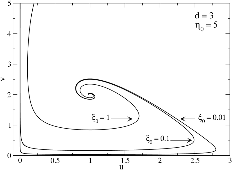
Figure 2: Solution of the Emden equation with a central body in the $(u,v)$ plane in $d=3$ dimensions (we have selected $\eta_{0}=5$ for illustration).

Let us introduce the analogue of the Milne variables

$$u=\frac{d\ln M_{\rm tot}(r)}{d\ln r},\qquad v=-\frac{d\ln P(r)}{d\ln r},$$ (49)

where $M_{\rm tot}(r)=M(r)+M_{*}$ is the total mass enclosed within the sphere of radius $r$ and $P(r)=\rho(r)k_{B}T/m$ is the local pressure. Using the equalities $GM_{\rm tot}(r)=r^{d-1}d\Phi_{\rm tot}/dr$ and $dM_{\rm tot}/dr=S_{d}r^{d-1}\rho(r)$ (see Appendix D), we easily find that

$$u=\frac{\xi e^{-\psi}}{\psi^{\prime}},\qquad v=\xi\psi^{\prime}.$$ (50)

Therefore, the Milne variables keep the same form as in the absence of central body chandrab . They satisfy the first order differential equation

$$\frac{u}{v}\frac{dv}{du}=\frac{2-d+u}{d-u-v}.$$ (51)

The $(u,v)$ curves are parameterized by $\xi$. They start from $(\xi_{0}^{2}/\eta_{0},\eta_{0})$ for $\xi=\xi_{0}$ and end at $(d-2,2)$ for $\xi\rightarrow+\infty$ (if $d>2$). An example of $(u,v)$ curve is shown in Fig. 2.

II.5 The thermodynamical parameters

For $d>2$, there is no global entropy maximum at fixed mass and energy in an unbounded domain. The isothermal gas surrounding the central body has the tendency to evaporate, leading to higher and higher values of entropy as the volume that it occupies increases. There are not even extrema of entropy at fixed mass and energy in an unbounded domain because the solutions of the Boltzmann-Poisson equation (24) have infinite mass. As in the case without central body, we shall confine the gas within a box of radius $R$. The box delimitates the region where the system is isolated from the surrounding so that thermodynamical arguments can be applied. It can mimic the effect of a tidal radius for globular clusters and dark matter halos, or represent the Hill sphere in the context of planet formation. In the context of the chemotaxis of bacterial populations, the box has a physical justification as it represents the domain containing the bacteria.

In a bounded domain, the solutions of the Emden equation (35) are terminated by the box at a normalized radius given by

$$\alpha=(S_{d}G\beta m\rho_{0})^{1/2}R.$$ (52)

Using Eqs. (8) and (52), we can rewrite Eq. (37) as

$$\xi_{0}=\alpha\zeta,\qquad\eta_{0}=\frac{\eta\mu}{\zeta^{d-2}}.$$ (53)

We shall now relate $\alpha$ to the dimensionless temperature $\eta$ and to the dimensionless energy $\Lambda$.

II.5.1 The temperature

According to the Newton law (30) applied at $r=R$, we have

$$\frac{d\Phi_{\rm tot}}{dr}(R)=\frac{G(M_{*}+M)}{R^{d-1}},$$ (54)

where $M$ is the total mass of the gas. Introducing the variables defined previously and using $\xi=r\alpha/R$, the foregoing relation can be rewritten as

$$\eta=\frac{\alpha\psi^{\prime}(\alpha)}{1+\mu}.$$ (55)

This relation can also be obtained by substituting the Boltzmann distribution (33) into the mass constraint (6) and by using the Emden equation (35).

II.5.2 The energy

The computation of the energy is a little more intricate. Using the Maxwell-Boltzmann distribution (21), or the isothermal equation of state (22), the kinetic energy

$$E_{\rm kin}=\int f\frac{v^{2}}{2}\,d{\bf r}d{\bf v}=\frac{d}{2}\int P\,d{\bf r}$$ (56)

is given by

$$E_{\rm kin}=\frac{d}{2}Nk_{B}T,$$ (57)

just like for a noninteracting (perfect) gas. Therefore, the dimensionless kinetic energy is

$$-\frac{E_{\rm kin}R^{d-2}}{GM^{2}}=-\frac{d}{2\eta}.$$ (58)

On the other hand, the potential energy $W_{\rm tot}=W+W_{\rm ext}$ is given by

$$W_{\rm tot}=\frac{1}{2}\int\rho\Phi\,d{\bf r}+\int\rho\Phi_{\rm ext}\,d{\bf r}.$$ (59)

Using Eq. (25) it can be rewritten as

$$W_{\rm tot}=\frac{1}{2}\int\rho\Phi_{\rm tot}\,d{\bf r}+\frac{1}{2}\int\rho\Phi_{\rm ext}\,d{\bf r}.$$ (60)

We shall compute the potential energy in two different manners, either by using the virial theorem or by directly evaluating the integral (60). The first approach based on the virial theorem is only valid for $d\neq 2$ while the second approach is general.

For $d\neq 2$, it is shown in Appendix B that the virial theorem for a self-gravitating gas in hydrostatic equilibrium surrounding a central body can be written as

$$2E_{\rm kin}+(d-2)W_{\rm tot}=dP(R)V-dP(R_{*})V_{*},$$ (61)

where $V=S_{d}R^{d}/d$ is the volume of the box enclosing the gas and $V_{*}=S_{d}R_{*}^{d}/d$ is the volume of the central body. This relation is valid for a general equation of state. For the isothermal equation of state (22), we obtain

$$2E_{\rm kin}+(d-2)W_{\rm tot}=S_{d}\left(\rho(R)R^{d}-\rho_{0}R_{*}^{d}\right)\frac{k_{B}T}{m},$$ (62)

where the first term (kinetic energy) is given by Eq. (57). This equation then determines the potential energy $W_{\rm tot}$. Introducing the dimensionless variables defined previously, we get

$$-\frac{W_{\rm tot}R^{d-2}}{GM^{2}}=\frac{\alpha^{2}}{(d-2)\eta^{2}}(\zeta^{d}-e^{-\psi(\alpha)})+\frac{d}{d-2}\frac{1}{\eta}.$$ (63)

The total energy is $E=E_{\rm kin}+W_{\rm tot}$. Adding Eqs. (58) and (63), we find that the total dimensionless energy is given by

$$\Lambda=\frac{4-d}{d-2}\frac{d}{2\eta}+\frac{\alpha^{2}}{(d-2)\eta^{2}}(\zeta^{d}-e^{-\psi(\alpha)})\quad(d\neq 2).$$ (64)

It can be useful to obtain another expression of the energy. Introducing the dimensionless variables defined previously in the expression of the potential energy (60), and using Eq. (98) for $d\neq 2$, we find that the dimensionless potential energy can be written as

$$-\frac{W_{\rm tot}R^{d-2}}{GM^{2}} = -\frac{1}{2\eta^{2}\alpha^{d-2}}\int_{\alpha\zeta}^{\alpha}(\psi+\psi_{*})e^{-\psi}\xi^{d-1}\,d\xi$$ (65)

$$+\frac{\mu}{2(d-2)\eta}\int_{\alpha\zeta}^{\alpha}e^{-\psi}\xi\,d\xi.$$

The quantity $\psi_{*}\equiv\beta m\Phi_{\rm tot}(R_{*})$ is obtained by evaluating $\psi(\xi)=\beta m\Phi_{\rm tot}(r)-\psi_{*}$ at $\xi=\alpha$, using $\Phi_{\rm tot}(R)=-[1/(d-2)]GM_{\rm tot}/R^{d-2}$ (see Appendix D) for $d\neq 2$. This yields

$$\psi_{*}=-\frac{\eta(1+\mu)}{d-2}-\psi(\alpha).$$ (66)

Adding Eqs. (58) and (65), we find that the total dimensionless energy is given by

$$\Lambda = -\frac{d}{2\eta}-\frac{1}{2\eta^{2}\alpha^{d-2}}\int_{\alpha\zeta}^{\alpha}(\psi+\psi_{*})e^{-\psi}\xi^{d-1}\,d\xi$$ (67)

$$+\frac{\mu}{2(d-2)\eta}\int_{\alpha\zeta}^{\alpha}e^{-\psi}\xi\,d\xi\qquad(d\neq 2).$$

This expression is equivalent to Eq. (64), but it is more complicated since it involves new integrals. However, the present method can be generalized in $d=2$ dimensions.

Using Eq. (99) for $d=2$, the dimensionless potential energy (60) can be written as

$$-\frac{W_{\rm tot}}{GM^{2}} = -\frac{1}{2\eta^{2}}\int_{\alpha\zeta}^{\alpha}(\psi+\psi_{*})e^{-\psi}\xi\,d\xi$$ (68)

$$-\frac{\mu}{2\eta}\int_{\alpha\zeta}^{\alpha}e^{-\psi}\ln(\xi/\alpha)\xi\,d\xi.$$

The quantity $\psi_{*}\equiv\beta m\Phi_{\rm tot}(R_{*})$ is obtained by evaluating $\psi(\xi)=\beta m\Phi_{\rm tot}(r)-\psi_{*}$ at $\xi=\alpha$, using $\Phi_{\rm tot}(R)=0$ (see Appendix D). This yields

$$\psi_{*}=-\psi(\alpha).$$ (69)

Adding Eqs. (58) and (68), we find that the total dimensionless energy is given by

$$\Lambda = -\frac{1}{\eta}-\frac{1}{2\eta^{2}}\int_{\alpha\zeta}^{\alpha}(\psi+\psi_{*})e^{-\psi}\xi\,d\xi+\frac{1}{2}\mu\ln\alpha$$ (70)

$$-\frac{\mu}{2\eta}\int_{\alpha\zeta}^{\alpha}e^{-\psi}\xi\ln\xi\,d\xi\qquad(d=2).$$

The virial theorem in $d=2$ is discussed in companion .

II.6 Entropy and free energy

The entropy and the free energy (or Massieu function) of the equilibrium state can be calculated as follows. From Eqs. (12) and (21) we get

$$S_{B}/k_{B}=\alpha_{0}M+\left(\frac{d}{2}+1\right)N+2\beta W+\beta W_{\rm ext},$$ (71)

where we have used Eqs. (56) and (57). Applying Eq. (23) at $r=R$ and using Eqs. (7), (33), (52) and $\Phi(R)+\Phi_{\rm ext}(R)=-G(M+M_{*})/[(d-2)R^{d-2}]$ for $d\neq 2$ or $\Phi(R)+\Phi_{\rm ext}(R)=0$ for $d=2$ [see Eqs. (98), (99), (150) and (151)], we find that

$$\alpha_{0}m=-2\ln\alpha-\left(\frac{d}{2}-1\right)\ln\eta+\psi(\alpha)+\frac{\eta}{d-2}(1+\mu)$$

$$+\ln\left[(2\pi)^{d/2}S_{d}G^{d/2}M^{(d-2)/2}mR^{(4-d)d/2}\right]-1.\qquad$$ (72)

We also have

$$E=\frac{d}{2}Nk_{B}T+W_{\rm tot}$$ (73)

with $W_{\rm tot}=W+W_{\rm ext}$. From Eqs. (7) and (73) we obtain

$$2\beta W+\beta W_{\rm ext}=-2N\Lambda\eta-dN-\beta W_{\rm ext}.$$ (74)

Substituting Eqs. (II.6) and (74) into Eq. (71) we find that

$$S_{B}/Nk_{B}=-\left(\frac{d}{2}-1\right)\ln\eta-2\ln\alpha+\psi(\alpha)$$

$$+\frac{1}{d-2}(1+\mu)\eta-2\Lambda\eta-\frac{d}{2}-\frac{\beta W_{\rm ext}}{N}$$

$$+\ln\left[(2\pi)^{d/2}S_{d}G^{d/2}M^{(d-2)/2}mR^{(4-d)d/2}\right].$$ (75)

The term $\beta W_{\rm ext}/N$ can be obtained from Eqs. (8), (33), (34), (53), (98) and (99) yielding

$$\frac{\beta W_{\rm ext}}{N}=-\frac{1}{d-2}\mu\int_{\alpha\zeta}^{\alpha}e^{-\psi}\xi\,d\xi\qquad(d\neq 2),$$ (76)

$$\frac{\beta W_{\rm ext}}{N}=\mu\int_{\alpha\zeta}^{\alpha}e^{-\psi}\ln({\xi}/{\alpha})\xi\,d\xi\qquad(d=2).$$ (77)

The Massieu function (14) is then given by

$$\frac{J_{B}}{N}=\frac{S_{B}}{Nk_{B}}+\Lambda\eta.$$ (78)

II.7 The structure of the gas profile close to the central body

In this section, we determine the profile of the gas in the vicinity of the central body. The density profile of the isothermal gas is given by the Boltzmann distribution

$$\rho(r)=Ae^{-\beta m\Phi_{\rm tot}(r)},$$ (79)

where $\Phi_{\rm tot}=\Phi+\Phi_{\rm ext}$ is the total gravitational potential. For $r\rightarrow R_{*}$, the gravitational potential is dominated by the contribution of the central body $\Phi_{\rm ext}(r)$ so that

$$\Phi_{\rm tot}({r})\simeq-\frac{1}{d-2}\frac{GM_{*}}{r^{d-2}}\qquad(d\neq 2),$$ (80)

$$\Phi_{\rm tot}(r)\simeq GM_{*}\ln(r/R)\qquad(d=2).$$ (81)

For $d=1$, we find that the density profile close to the central body increases exponentially rapidly as

$$\rho(x)=\rho_{0}e^{-({x}-{R_{*}})/\epsilon}$$ (82)

on a typical length scale

$$\epsilon=\frac{1}{\beta GmM_{*}}.$$ (83)

This corresponds to a “cusp” since the first derivative $\rho^{\prime}(R_{*})=-\rho_{0}/\epsilon$ of the density profile is nonzero at $x=R_{*}$. This solution remains valid if the central body is a Dirac mass ($R_{*}=0$) in which case $\rho=\rho_{0}e^{-x/\epsilon}$ for $x\rightarrow 0$ companion .

For $d=2$, we find that the density profile close to the central body increases like a power law:

$$\rho(r)=\rho_{0}\left(\frac{R_{*}}{r}\right)^{\beta GM_{*}m}.$$ (84)

Again, we have a cusp since $\rho^{\prime}(R_{*})=-\beta GM_{*}m\rho_{0}/R_{*}\neq 0$. This power-law behavior remains valid if the central body is a Dirac mass ($R_{*}=0$) in which case $\rho(r)=Ar^{-\beta GM_{*}m}$. The density diverges at $r=0$ and the profile is normalizable provided that $\beta GM_{*}m<2$ companion .

For $d=3$, we find that the density profile close to the central body is

$$\rho(r)=\rho_{0}e^{\beta GM_{*}m\left(\frac{1}{r}-\frac{1}{R_{*}}\right)}.$$ (85)

We note that the density profile is not normalizable in the case where the central body is a Dirac mass ($R_{*}=0$). For $r\rightarrow R_{*}$, we find that the density profile increases exponentially rapidly as

$$\rho(r)=\rho_{0}e^{-(r-R_{*})/\epsilon}$$ (86)

on a typical length scale

$$\epsilon=\frac{R_{*}^{2}}{\beta GM_{*}m}.$$ (87)

Therefore, at the contact with the central body, there is a density spike (or cusp) of the gas on a typical length $\epsilon$ since $\rho^{\prime}(R_{*})=-\rho_{0}/\epsilon\neq 0$. Then, taking $r\rightarrow+\infty$ in Eq. (85), we find that the spike is followed by a plateau where the density is nearly constant:

$$\rho=\rho_{0}e^{-\frac{\beta GM_{*}m}{R_{*}}}.$$ (88)

This plateau extends on a typical length $L$ such that the mass of gas contained in this region becomes comparable to the mass of the central body. This corresponds to the condition

$$\rho_{0}e^{-\frac{\beta GM_{*}m}{R_{*}}}\frac{4}{3}\pi(L^{3}-R_{*}^{3})=M_{*}.$$ (89)

If $R_{*}\ll L$, we get the estimate

$$L\simeq\left(\frac{3M_{*}}{4\pi\rho_{0}}\right)^{1/3}e^{\frac{\beta GM_{*}m}{3R_{*}}}.$$ (90)

For $r>L$, the self-gravity of the gas must be taken into account and, at large distances, the density decreases with a typical $r^{-2}$ behavior corresponding to the standard self-gravitating isothermal sphere chandrab . This “cusp $+$ plateau $+$ halo” structure (or simply “cusp-halo” structure) is clearly visible in Fig. 1. These results are similar to those found in the case of self-gravitating fermions mnras ; ptfermi where the role of the central body is played by the completely degenerate fermion ball (quantum core).

From these considerations, we can distinguish four types of configurations which are reminiscent of the morphology of certain objects in planetology:

(i) If the mass of the central body is small (or if there is no central body) and if the gas is not too dense we have a non-self-gravitating homogeneous gas that could represent a diffuse nebula.

(ii) If the mass of the central body is large and if the gas is not too dense we have a non-self-gravitating gas experiencing only the gravitational potential of the central body (solid planetary core). The density of the gas increases rapidly at the contact of the solid core and forms a spike. A massive solid core surrounded by a tiny atmosphere corresponds to the structure of telluric planets like the Earth.

(iii) If the mass of the central body is small (or if there is no central body) and if the gas is sufficiently dense we have a standard isothermal self-gravitating gas (isothermal sphere) with a finite central density. It could represent a protoplanet.

(iv) If the mass of the central body is large and if the gas is sufficiently dense we have a self-gravitating gas experiencing the gravitational potential of the central body (solid planetary core). The density of the gas increases rapidly at the contact of the solid core and forms a spike. This thin layer is then followed by an envelope held by its self-gravity. This corresponds to the structure of giant planets like Jupiter and Saturn.

Cases (i) and (iii) correspond to the “gaseous phase” where the influence of the central object is weak. Cases (ii) and (iv) correspond to the “condensed phase” where the influence of the central object is strong. In that case, the density of the gas is enhanced close to the solid core and forms a spike. The gaseous phase and the condensed phase can themselves be divided in two categories depending on whether the envelope is self-gravitating or not.

The case of globular clusters and dark matter halos, which are self-gravitating, corresponds to points (iii) and (iv) depending whether they contain a central black hole or not.

II.8 The numerical procedure

In order to plot the series of equilibria $\eta(\Lambda)$ for fixed external parameters $\zeta$ and $\mu$, we proceed as follows: (i) We fix $\xi_{0}$ and make a guess $\eta_{0}^{\rm guess}$ for $\eta_{0}$; (ii) we solve the Emden equation (35) with the boundary condition from Eq. (36) until $\alpha=\xi_{0}/\zeta$. This gives $\eta$ and $\Lambda$ according to the formulae of Sec. II.5 and $\eta_{0}=\eta\mu/\zeta^{d-2}$. We iterate this procedure until the values of $\eta_{0}^{\rm guess}$ and $\eta_{0}$ coincide; (iii) in that case, the chosen value of $\xi_{0}$ determines $\alpha$, $\eta$ and $\Lambda$. By varying $\xi_{0}$, we can obtain the whole series of equilibria $\eta(\Lambda)$ for given values of $\zeta$ and $\mu$.

III Caloric curves and phase transitions in the presence of a central body in $d=3$ dimensions

In this section, we describe phase transitions which take place in a self-gravitating system with a central body in $d=3$ dimensions. We fix the typical density of the central body, $\rho_{*}=M_{*}/R_{*}^{3}$, and plot the series of equilibria $\beta(E)$ for different values of the radius $R_{*}$ of the central body. We could also fix the mass $M_{*}$ of the central body instead of its average density, but we think that fixing the average density is more relevant if we want to apply our results, for example, to the problem of planet formation. Furthermore, the classical isothermal gas without central body antonov ; lbw is recovered for $R_{*}\rightarrow 0$ with fixed $\rho_{*}$ while the limit $R_{*}\rightarrow 0$ with fixed $M_{*}$ corresponds to a central Dirac mass. This corresponds to a very different situation.

The dimensionless density of the central body is

$$\kappa\equiv\frac{M_{*}R^{3}}{MR_{*}^{3}}=\frac{\mu}{\zeta^{3}}.$$ (91)

We shall work with the dimensionless variables defined previously. However, it may be useful in the discussion to take $M=R=G=m=1$ (we can always introduce appropriate scales to be in this situation). In that case, $\zeta=R_{*}$ represents the radius of the central body, $\kappa=\rho_{*}$ the density of the central body, $\eta=\beta$ the inverse temperature of the gas and $\Lambda=-E$ the energy of the gas (with the opposite sign). In the discussion, we shall use the physical variables $R_{*}$, $\rho_{*}$, $\beta$ and $E$, and in the figures, we shall use the dimensionless variables $\zeta$, $\kappa$, $\eta$ and $\Lambda$.

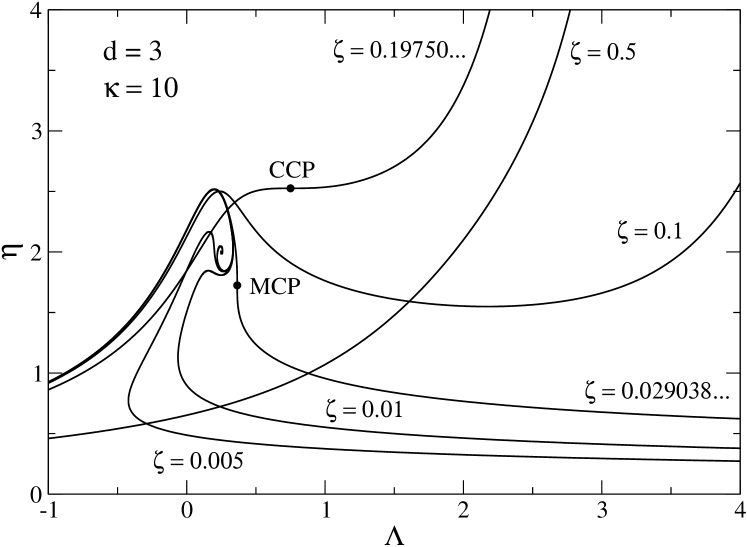
Figure 3: Series of equilibria at fixed central body density $\kappa$ (we have taken $\kappa=10$ for illustration) for several values of the central body radius $\zeta$. As $\zeta$ increases, the series of equilibria unwinds. There exists a microcanonical critical point (MCP) and a canonical critical point (CCP) above which the microcanonical and the canonical phase transitions respectively disappear.

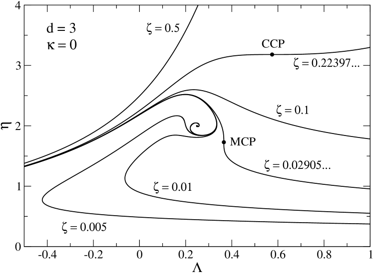
Figure 4: Same as Fig. 3 for $\kappa=0$ and $\zeta\neq 0$ (hole). This corresponds to a system of self-gravitating particles contained in a volume delimited by two shells at radii $r=R_{*}$ and $r=R$.

In Figs. 3 and 4, we plot the curve $\beta(E)$ for a fixed central body density $\rho_{*}$ and for different values of the central body radius $R_{*}$. This curve contains all the extrema of entropy (resp. free energy) at fixed mass and energy (resp. temperature). For that reason, it is called the series of equilibria. The series of equilibria is parameterized by the density contrast ${\cal R}=\rho_{0}/\rho(R)=e^{\psi(\alpha)}$ between the central body and the box. The stable part of this curve in each ensemble defines the caloric curve. The series of equilibria (extremal states) is the same in the canonical and microcanonical ensembles while the caloric curve (stable states) can be different in case of ensemble inequivalence. For $R_{*}\rightarrow 0$, we recover the classical spiral of a self-gravitating isothermal gas without central body paddy ; dvs1 ; dvs2 ; katzrevue ; ijmpb . For finite $R_{*}$, the spiral unwinds and different shapes are possible depending on the value of $R_{*}$. For $R_{*}<R_{*}^{\rm MCP}$, the curve has a $Z$-shape structure leading to zeroth and first order microcanonical and canonical phase transitions. At the microcanonical critical point $R_{*}=R_{*}^{\rm MCP}$, the microcanonical phase transitions disappear. For $R_{*}^{\rm MCP}<R_{*}<R_{*}^{\rm CCP}$, the curve has an $N$-shape structure leading to zeroth and first order canonical phase transitions. At the canonical critical point $R_{*}=R_{*}^{\rm CCP}$, the canonical phase transitions disappear. Finally, for $R_{*}>R_{*}^{\rm CCP}$, the curve is monotonic so that there is no phase transition anymore. In that case, the statistical ensembles are equivalent.

We see that the description of phase transitions in a self-gravitating classical gas with a central body is very similar to that already given for self-gravitating fermions ijmpb . The central body provides a small scale regularization of the gravitational force that prevents complete collapse and the formation of singularities. In that sense, it has an effect similar to the Pauli exclusion principle in quantum mechanics or to the core radius of the particles in a hard spheres gas. Since the phenomenology is the same in all these situations, we shall be relatively brief and refer to the review ijmpb for more details about phase transitions in self-gravitating systems. We note, however, that in the present case, the structure of the series equilibria $\beta(E)$ depends on two parameters $\rho_{*}$ and $R_{*}$ characterizing the central body while in the case of self-gravitating fermions there is only one parameter $\mu=(gm^{4}/h^{3})\sqrt{512\pi^{4}G^{3}MR^{3}}$ related to the inverse of the Planck constant ($\mu\sim 1/\hbar^{3}$) or to the ratio $\mu\sim(R/R_{*})^{3/2}$ between the system size $R$ and the size $R_{*}$ of a fermion ball (a self-gravitating Fermi gas at $T=0$) with mass $M$. Furthermore, in the present case, the central body is an external object distinct from the gas while the fermion ball (or the solid core) is created by the system itself. What plays the role of the condensed object in the present context is the cusp at the contact with the central body (there is also a cusp in the case of self-gravitating fermions mnras ).

III.1 The case of a small central body $R_{*}<R_{*}^{\rm MCP}$ in the microcanonical ensemble: $Z$-shape structure

We first consider the case of a small central body $R_{*}<R_{*}^{\rm MCP}$ so that the series of equilibria has a $Z$-shape structure resembling a “dinosaur’s neck” ijmpb (see Figs. 5 and 6).

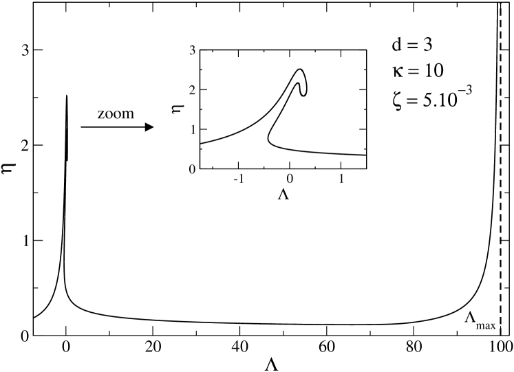
Figure 5: Series of equilibria for $\kappa=10$ and $\zeta=5\times 10^{-3}<\zeta_{\rm MCP}$. It has a characteristic $Z$-shape structure (“dinosaur’s neck” ijmpb ). There exists an equilibrium state for all accessible values of the energy $\Lambda\leq\Lambda_{\rm max}(\zeta,\kappa)$ in the microcanonical ensemble, and for all values of temperature $\eta\geq 0$ in the canonical ensemble. However, interesting phase transitions, described in the text, appear for energies around $\Lambda_{c}$ and temperatures around $\eta_{c}$ (see the following figures).

In this section, we consider the case of an isolated system so that the control parameter is the energy and the relevant statistical ensemble is the microcanonical ensemble. As explained previously, the series of equilibria contains all the extrema of entropy at fixed mass and energy. The thermodynamically stable states in the microcanonical ensemble correspond to entropy maxima at fixed mass and energy (minima or saddle points of entropy must be discarded). They can be determined by applying the turning point method of Poincaré (see, e.g. katzrevue ; ijmpb ). At very high energies, self-gravity is negligible with respect to thermal motion (velocity dispersion) and the system is equivalent to a non-interacting gas in a box. We know from ordinary thermodynamics that this gas is stable (entropy maximum). Therefore, using the Poincaré criterion, we conclude that the upper branch of the series of equilibria is stable (entropy maxima at fixed mass and energy) until the first turning point of energy $E_{c}$ where the tangent is vertical. For sufficiently small values of $R_{*}$, this is close to the Antonov energy $-0.335$ antonov ; paddy . At that point, the curve $\beta(-E)$ rotates clockwise so that a mode of stability is lost. Therefore, the configurations in the intermediate branch are unstable saddle points of entropy at fixed mass and energy. However, at the second turning point of energy $E_{*}$, the curve $\beta(-E)$ rotates anti-clockwise so that the mode of stability is regained. Therefore, the lower branch is stable (entropy maxima at fixed mass and energy). The energy $E_{*}$ depends on $R_{*}$ and tends to $E_{*}(R_{*})\rightarrow+\infty$ when $R_{*}\rightarrow 0$.

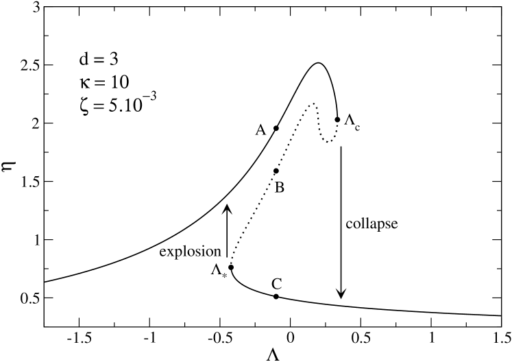
Figure 6: Physical caloric curve in the microcanonical ensemble (solid lines) containing stable (global entropy maxima) and metastable (local entropy maxima) equilibrium states. Unstable saddle points of entropy are represented by dotted lines.

Typical density profiles of the series of equilibria are shown in Fig. 7. The states (A) on the upper branch have an almost uniform density with a small density contrast ${\cal R}=\rho(R_{*})/\rho(R)$. They form the gaseous phase. At large distances, their density profile decreases approximately like $r^{-2}$. The states (C) on the lower curve are highly inhomogeneous. They present a high-density cusp at the contact with the central body surrounded by a dilute atmosphere. Therefore the density contrast ${\cal R}=\rho(R_{*})/\rho(R)$ is large. They form the condensed phase. They have a “cusp-halo” structure which is the counterpart of the “core-halo” structure of self-gravitating fermions (in that case the core is a degenerate quantum body). The cusp contains a lot of potential energy. By forming the cusp, some energy is released in the form of kinetic energy in the halo which is very hot and almost uniform. This explains the plateau following the cusp (see Sec. II.7). Finally, the states (B) on the intermediate (unstable) branch are similar to the gaseous states (the density profile decreases approximately like $r^{-2}$ at large distances) except that they form an embryonic cusp at the contact with the core. This is the equivalent of a “germ” in the language of phase transitions (see below).

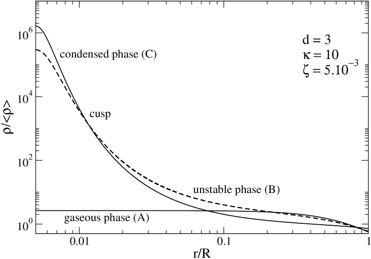
Figure 7: Typical normalized density profiles $\rho/\langle{\rho}\rangle$ with $\langle{\rho}\rangle=3M/4\pi R^{3}$ corresponding to gaseous (points $A$), condensed (points $C$) and unstable (points $B$) states. The condensed and unstable states have a cusp-halo structure.

In Fig. 8, we have plotted the inverse temperature $\beta$ and minus the energy $-E$ as a function of the central density $\rho_{0}=\rho(R_{*})$ (more precisely the value of the density of the gas at the contact with the central body). The central density parameterizes the series of equilibria. We clearly see the appearance of oscillations giving rise to the spiral on the series of equilibria. They lead to microcanonical instability at the first turning point of energy and to canonical instability at the first turning point of temperature (stability is regained at the last turning points).

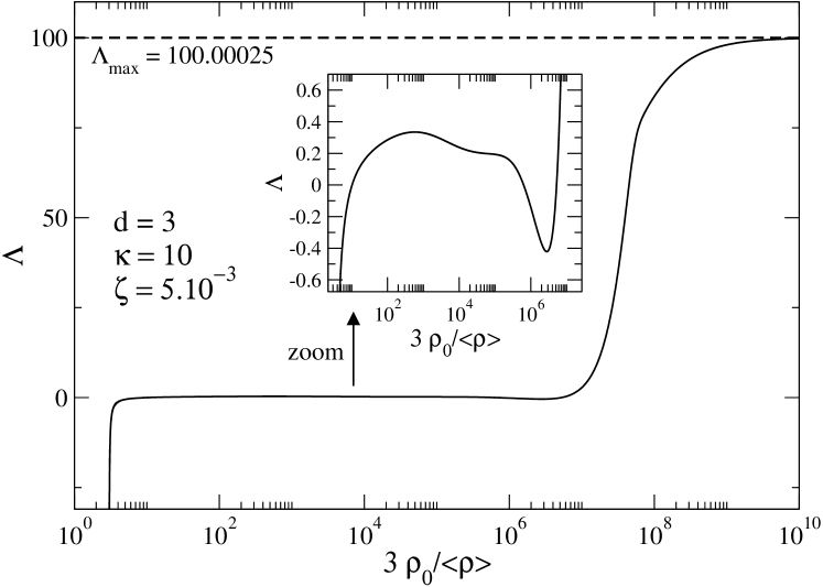
(a)    (b)

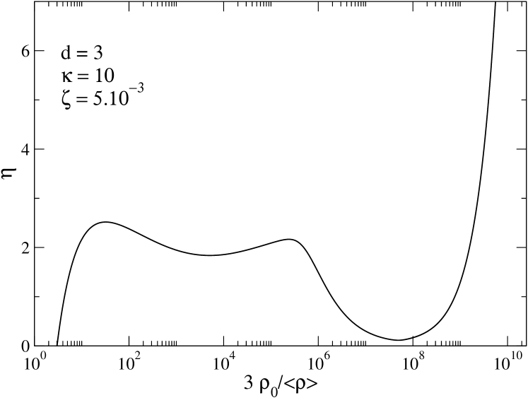
Figure 8: Evolution of the energy $\Lambda$ and the inverse temperature $\eta$ as a function of the normalized central density $\rho_{0}/\langle{\rho}\rangle$.

In principle, to obtain the caloric curve, we must determine which states are local entropy maxima and which states are global entropy maxima. This can be done by performing a vertical Maxwell construction or by plotting the entropy of the two phases as a function of the energy and determining the transition energy $E_{t}$ at which they become equal ijmpb . The strict caloric curve in the microcanonical ensemble is obtained by keeping only fully stable states (global entropy maxima), as in Fig. 9. From this curve, we would expect a first order microcanonical phase transition to occur at $E=E_{t}$, connecting the gaseous phase to the condensed phase. It would be accompanied by a discontinuity of temperature and specific heat. However, for self-gravitating systems, the metastable states are long-lived because the probability of a fluctuation able to trigger the phase transition is extremely weak. Indeed, in order to trigger a phase transition between a gaseous state and a condensed state, the system has to overcome the entropic barrier played by the solution of the intermediate branch (points B) with a “germ”. Now, the height of the entropic barrier scales like $N$ so that the probability of transition scales like $e^{-N}$. Therefore, metastable states (local entropy maxima) are very robust lifetime because their lifetime scales like the exponential of the number of particles, $t_{\rm life}\sim e^{N}$, and it becomes infinite at the thermodynamic limit $N\rightarrow+\infty$. In practice, the first order phase transition at $E_{t}$ does not take place and, for sufficiently large $N$, the system remains “frozen” in the metastable phase. Therefore, the physical caloric curve in the microcanonical ensemble must take into account the metastable states (local entropy maxima) which are as much relevant as the fully stable equilibrium states (global entropy maxima). This physical caloric curve is multi-valued and corresponds to the solid lines in Fig. 6. It is obtained from the series of equilibria by discarding the unstable saddle points (dashed line).

Figure 9: Caloric curve in the microcanonical ensemble. We have indicated the fully stable states (global entropy maxima S), the metastable states (local entropy maxima M) and the unstable states (saddle points U). The strict caloric curve is composed by the fully stable states and exhibits a first order phase transition at $\Lambda_{t}$. In practice, this phase transition does not take place because the metastable states have a very long lifetime. The physical caloric curve is composed of the fully stable and metastable states (see Fig. 6). The ends of the metastable branches are called spinodal points. At these points, the system exhibits zeroth order phase transitions associated with a collapse and an explosion.

Reducing progressively the energy from high values (for unbounded systems, the mechanism by which energy decreases may be due physically to a slow evaporation), the system remains in the gaseous phase (points $A$) until the critical value $E_{c}$ at which the gaseous phase ceases to exist. At that point, called a spinodal point, the system undergoes a gravothermal catastrophe lbw . However, in the present case, complete collapse is prevented by the central body and the systems ends up in the condensed phase (points $C$). Since the gravitational collapse is accompanied by a discontinuous jump of entropy this phase transition is of zeroth order. The resulting equilibrium state has a “cusp-halo” structure. The cusp contains a small fraction of the mass and this fraction decreases as $R_{*}\rightarrow 0$ (in the absence of a central body, the gravothermal catastrophe leads to a binary star with a small mass but a large binding energy ijmpb ). The rest of the mass is diluted in a hot and massive envelope held by the box. In an open system (i.e., if the box is removed) the halo would be dispersed at infinity so that only the cusp (thin atmosphere) would remain. If we now increase the energy of the gas (for unbounded systems, the mechanism to supply energy could be due to an accretion), the system remains in the condensed phase until the critical value $E_{*}$ at which the condensed phase ceases to exist. At that second spinodal point, the system undergoes an explosion, reverse to the collapse, and returns to the gaseous phase. Since the collapse and the explosion occur at different values of the energy (due to the presence of metastable states), we can generate an hysteretic cycle in the microcanonical ensemble by varying the energy between $E_{c}$ and $E_{*}$. This hysteretic cycle has been followed numerically by Ispolatov and Karttunen ik for particles interacting via a softened gravitational potential (the softening regularizes the singularity of the gravitational potential and plays a role similar to that of the central body in our case).

III.2 The case of a moderate central body $R_{*}^{\rm MCP}<R_{*}<R_{*}^{\rm CCP}$ in the microcanonical ensemble: $N$-shape structure

We now consider the case of a central body of intermediate core radius, $R_{*}^{\rm MCP}<R_{*}<R_{*}^{\rm CCP}$, so that the series of equilibria has an $N$-shape structure (see Fig. 10).

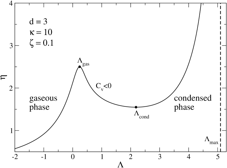
Figure 10: Caloric curve in the microcanonical ensemble for $\kappa=10$ and $\zeta_{\rm MCP}<\zeta=0.1<\zeta_{\rm CCP}$. It has a characteristic $N$-shape structure. All the solutions are global entropy maxima at fixed mass and energy (fully stable). The solutions between $\Lambda_{\rm gas}$ and $\Lambda_{\rm cond}$ have negative specific heats. There is no phase transition in the microcanonical ensemble, only a concentration of the gas near the central body as energy is progressively decreased.

We first describe the structure of the caloric curve in the microcanonical ensemble. In that case, the control parameter is the energy $E$. For a moderate value of the core radius, the trace of the classical spiral has almost disappeared and the $\beta(E)$ curve is univalued. Since the solutions are entropy maxima for $E\rightarrow+\infty$, and since there is no turning point of energy (no vertical tangent) in the series of equilibria, we conclude from the Poincaré criterion that all the states are stable and correspond to global entropy maxima at fixed mass and energy. Therefore, for sufficiently large values of the core radius, there is no phase transition in the microcanonical ensemble. The gravothermal catastrophe at $E_{c}$ is suppressed. However, there is a sort of condensation as the energy is progressively decreased. At high energies, the density profiles are almost homogeneous and they are held by the box. In that case, the specific heat is positive. At smaller energies, the density contrast increases and the system has a “cusp-halo” structure. Between $E_{\rm gas}$ and $E_{\rm cond}$, the influence of the central body and of the box are weak and these states have negative specific heats. Finally, at low energies, the cusp becomes more and more massive and thin until the minimum energy $E_{\rm min}$ at which all the mass is in contact with the central body (see Appendix F). In that case, the specific heat is positive again.

III.3 The case of a moderate central body $R_{*}^{\rm MCP}<R_{*}<R_{*}^{\rm CCP}$ in the canonical ensemble: $N$-shape structure

We now describe the structure of the caloric curve in the canonical ensemble for the same values of the parameters as in the previous section. In that case, the control parameter is the temperature $T$ and the reader may find useful to rotate Fig. 10 by $90^{\rm o}$ to have the control parameter $\eta\sim 1/T$ in abscissa. The series of equilibria $E(T)$ is multi-valued and this gives rise to canonical phase transitions (see Fig. 11). In fact, we are in a situation parallel to the one described in Sec. III.1 in the microcanonical ensemble, provided that we interchange the role of $E$ and $T$. The series of equilibria contains all the extrema of free energy at fixed mass. The thermodynamically stable states in the canonical ensemble correspond to free energy minima at fixed mass (maxima or saddle points of free energy must be discarded). They can be determined by applying the turning point method of Poincaré. At very high temperatures, self-gravity is negligible with respect to thermal motion and the system is equivalent to a non-interacting gas in a box. We know from ordinary thermodynamics that this gas is stable in every ensemble. Therefore, using the Poincaré criterion, we conclude that the left branch is stable (free energy minima at fixed mass) until the first turning point of temperature $T_{c}$ where the tangent is horizontal. For sufficiently small values of $R_{*}$, this is close to the Emden inverse temperature $2.52$ emden ; aa1 . At that point, the curve $-E(\beta)$ rotates clockwise so that a mode of stability is lost. Therefore, the configurations in the intermediate branch are unstable saddle points of free energy. They lie in the region of negative specific heats which is forbidden (unstable) in the canonical ensemble. However, at the second turning point of temperature $T_{*}$, the curve $-E(\beta)$ rotates anti-clockwise so that the mode of stability is regained. Therefore, the right branch is stable (free energy minima at fixed mass). The temperature $T_{*}$ depends on $R_{*}$ and tends to $T_{*}(R_{*})\rightarrow+\infty$ when $R_{*}\rightarrow 0$.

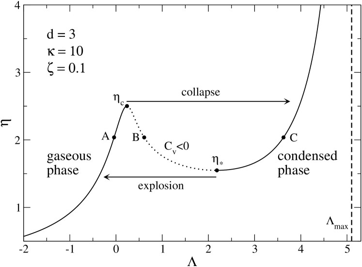
Figure 11: Physical caloric curve in the canonical ensemble (solid lines) containing stable (global free energy minima) as well as metastable (local free energy minima) equilibrium states. Unstable saddle points of free energy at fixed mass are represented by dotted lines and they lie in the region of negative specific heats.

Typical density profiles of the series of equilibria are shown in Fig. 12. The states (A) on the left branch have almost uniform density profiles and they form the gaseous phase. The states (C) on the right branch are highly inhomogeneous with a cusp-halo structure. They form the condensed phase. Finally, the states (B) on the intermediate (unstable) branch are similar to the gaseous states except that they contain an embryonic cusp at the contact with the central body. This is the equivalent of a “germ” in the language of phase transitions.

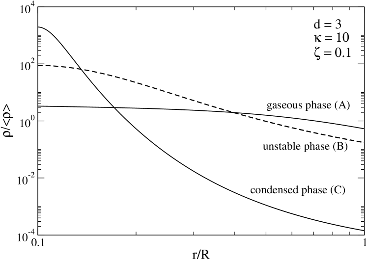
Figure 12: Typical normalized density profiles $\rho/\langle{\rho}\rangle$ corresponding to gaseous (points $A$), condensed (points $C$) and unstable (points $B$) states.

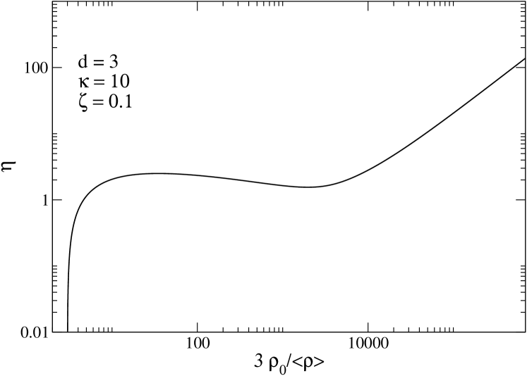
(a)    (b)

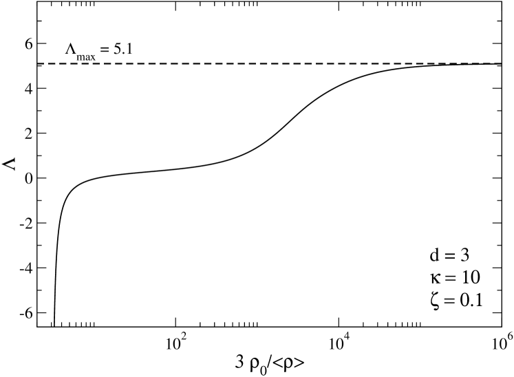
Figure 13: Evolution of the dimensionless energy $\Lambda$ and inverse temperature $\eta$ as a function of the normalized central density $\rho_{0}/\langle{\rho}\rangle$.

In Fig. 13, we have plotted the inverse temperature $\beta$ and minus the energy $-E$ as a a function of the central density $\rho_{0}=\rho(R_{*})$ (more precisely the value of the density of the gas at the contact with the central body). The central density parameterizes the series of equilibria. We clearly see the oscillations of $T(\rho_{0})$ giving rise to canonical instability at the first turning point of temperature (stability is regained at the last turning point of temperature). On the other hand, the absence of oscillations of $E(\rho_{0})$ is associated to full stability in the microcanonical ensemble (see Sec. III.3).

In principle, to obtain the caloric curve, we must determine which states are local free energy minima and which states are global free energy minima. This can be done by performing a horizontal Maxwell construction or by plotting the free energy of the two phases as a function of the temperature and determining the transition temperature $T_{t}$ at which they become equal. The strict caloric curve in the canonical ensemble is obtained by keeping only fully stable states (global free energy minima) as in Fig. 14. From this curve, we would expect a first order canonical phase transition to occur at $T=T_{t}$, connecting the gaseous phase to the condensed phase. It would be accompanied by a discontinuity of energy and specific heat. Therefore, the region of negative specific heats in the microcanonical ensemble (see Fig. 10) would be replaced by a phase transition (plateau) in the canonical ensemble (see Fig. 14). However, for self-gravitating systems, the metastable states are long-lived because the probability of a fluctuation able to trigger the phase transition is extremely weak. Indeed, in order to trigger a phase transition between a gaseous state and a condensed state, the system has to overcome the barrier of free energy played by the solutions of the intermediate branch (points B) with a “germ”. Yet, the height of the barrier of free energy scales like $N$ so that the probability of transition scales like $e^{-N}$. Therefore, metastable equilibrium states (local free energy minima) are very robust lifetime because their lifetime scales like the exponential of the number of particles, $t_{\rm life}\sim e^{N}$, and it becomes infinite at the thermodynamic limit $N\rightarrow+\infty$. In practice, the first order phase transition at $T_{t}$ does not take place and, for sufficiently large $N$, the system remains “frozen” in the metastable phase. Therefore, the physical caloric curve in the canonical ensemble must take into account the metastable states (local free energy minima) which are as much relevant as the fully stable equilibrium states (global free energy minima). This physical caloric curve is multi-valued and corresponds to the solid lines in Fig. 11. It is obtained from the series of equilibria by discarding the unstable saddle points (dashed line).

Figure 14: Caloric curve in the canonical ensemble. We have indicated the fully stable states (global free energy minima S), the metastable states (local free energy minima M) and the unstable states (saddle points U). The strict caloric curve is composed by the fully stable states and exhibits a first order phase transition at $\eta_{t}$ which replaces the region of negative specific heats allowed in the microcanonical ensemble (see Fig. 10). In practice, this phase transition does not take place because the metastable states have a very long lifetime. The physical caloric curve is composed of the fully stable and metastable states (see Fig. 11). The ends of the metastable branches are called spinodal points. At these points, the system exhibits zeroth order phase transitions associated with a collapse and an explosion.

Reducing progressively the temperature from high values, the system remains in the gaseous phase (points $A$) until the critical value $T_{c}$ at which the gaseous phase ceases to exist. At that point, called a spinodal point, the system undergoes an isothermal collapse aa1 . However, in the present case, complete collapse is prevented by the central body and the systems ends up in the condensed phase (points $C$). Since the gravitational collapse is accompanied by a discontinuous jump of free energy, this phase transition is of zeroth order. The resulting equilibrium state has a “cusp-halo” structure. The cusp contains a large fraction of the mass and this fraction increases as $R_{*}\rightarrow 0$ (in the absence of a central body, the isothermal collapse leads to a Dirac peak containing all the mass ijmpb ). The rest of the mass is diluted in a light envelope held by the box. In an open system (i.e., if the box is removed) the halo would be dispersed to infinity so that only the cusp (thin atmosphere) would remain. If we now increase the temperature of the gas, the system remains in the condensed phase until the critical value $T_{*}$ at which the condensed phase ceases to exist. At that second spinodal point, the system undergoes an explosion, reverse to the collapse, and returns to the gaseous phase. Since the collapse and the explosion occur at different values of the temperature (due to the presence of metastable states), one can generate an hysteretic cycle in the canonical ensemble by varying the temperature between $T_{c}$ and $T_{*}$. This hysteretic cycle has been followed numerically by Chavanis et al. crrs for a self-gravitating Fermi gas (as we have already indicated, the Pauli exclusion principle plays a role similar to that of the central body in our case).

III.4 The case of a large central body $R_{*}>R_{*}^{\rm CCP}$: monotonicity and equivalence of statistical ensembles

We now consider the case of a large central body $R_{*}>R_{*}^{\rm CCP}$ so that the series of equilibria is monotonic (see Fig. 15). In that case, the system does not present any phase transition and the ensembles are equivalent.

Figure 15: Caloric curve for $\kappa=10$ and $\zeta=0.5>\zeta_{\rm CCP}$. It is monotonic and the ensembles are equivalent.

III.5 The case of a small central body $R_{*}<R_{*}^{\rm MCP}$ in the canonical ensemble: multi-rotations

For a small central body $R_{*}<R_{*}^{\rm MCP}$, the system can display both microcanonical and canonical phase transitions (zeroth and first order). The microcanonical caloric curve has been described in Sec. III.1. Let us describe the corresponding caloric curve in the canonical ensemble. The series of equilibria displays several turning points of temperature (see Fig. 16). At the first turning point $T_{c}$, the curve rotates clockwise so that a mode of stability is lost. At the second turning point of temperature, another mode of stability is lost. At the third turning point of temperature, the curve rotates anti-clockwise so that the second mode is regained and at the fourth turning point of temperature $T_{*}$ the first mode is regained. Therefore, the left branch (before $T_{c}$) and the right branch (after $T_{*}$) are canonically stable (free energy minima) and form the physical canonical caloric curve. Although the structure of the series of equilibria in the unstable domain is more complex than in Sec. III.2, because it displays several rotations, the caloric curve corresponding to the stable part of the series of equilibria is simple and similar to Fig. 11 obtained for a larger value of the core radius. The strict canonical caloric curve containing only fully stable states (global free energy minima) would also be similar to Fig. 14.

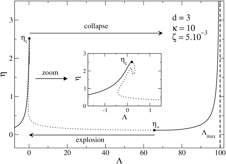
Figure 16: Physical canonical caloric curve for $\zeta=5\times 10^{-3}<\zeta_{\rm MCP}$ and $\kappa=10$. The dotted lines represent the unstable states (saddle points).

III.6 The limit of a vanishing central body $R_{*}\rightarrow 0$

It is of interest to study the limit of a vanishing central body $R_{*}\rightarrow 0$ in order to make the connection with the classical studies of Antonov antonov , Lynden-Bell and Wood lbw , and Katz katzpoincare1 .

As the radius of the central body decreases, the series of equilibria winds up several times before unwinding so that more and more turning points of energy and temperature appear. This is illustrated in Figs. 17 and 18. However, the discussion concerning the phase transitions remains essentially unchanged. In the microcanonical ensemble, the gaseous phase (upper branch) is stable until the energy $E_{c}$ and the condensed phase (lower branch) is stable from the energy $E_{*}$. In the canonical ensemble, the gaseous phase (left branch) is stable until the temperature $T_{c}$ and the condensed phase (right branch) is stable from the temperature $T_{*}$. When $R_{*}\rightarrow 0$, the energy $E_{*}\rightarrow-\infty$ and the temperature $T_{*}\rightarrow+\infty$. Similarly, $E_{t}\rightarrow-\infty$ and $T_{t}\rightarrow+\infty$. Therefore, the gaseous branch only contains metastable states. The condensed branch in the microcanonical ensemble approaches the $\beta=0$ axis and is formed by configurations presenting a thin cusp containing a weak mass but a large potential energy surrounded by a hot and massive halo (in the absence of a central body, the gravothermal catastrophe leads to a tight binary star surrounded by a very hot halo with a very large entropy). The condensed branch in the canonical ensemble is rejected to $E\rightarrow-\infty$ and is formed by configurations presenting a thin cusp containing most of the mass (in the absence of a central body, the isothermal collapse leads to a Dirac peak containing all the mass and having a very negative free energy). The unstable branch makes several oscillations and leads to the classical spiral discussed by Antonov antonov , Lynden-Bell and Wood lbw , and Katz katzpoincare1 .

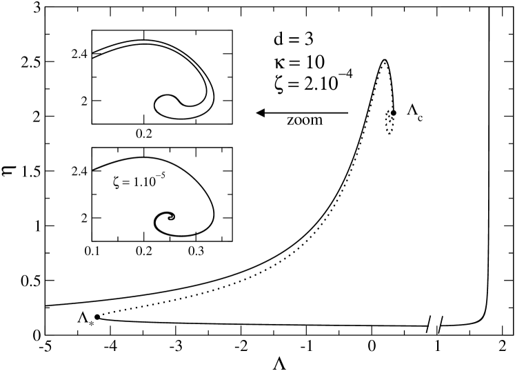
Figure 17: Series of equilibria at fixed $\kappa=10$ for several small values of $\zeta$. As $\zeta\rightarrow 0$, the series of equilibria makes more and more rotations around the singular sphere $(\Lambda,\eta)=(1/4,2)$ before unwinding (see inset). When $\zeta=0$, we recover the classical spiral of a spherical isothermal self-gravitating system.

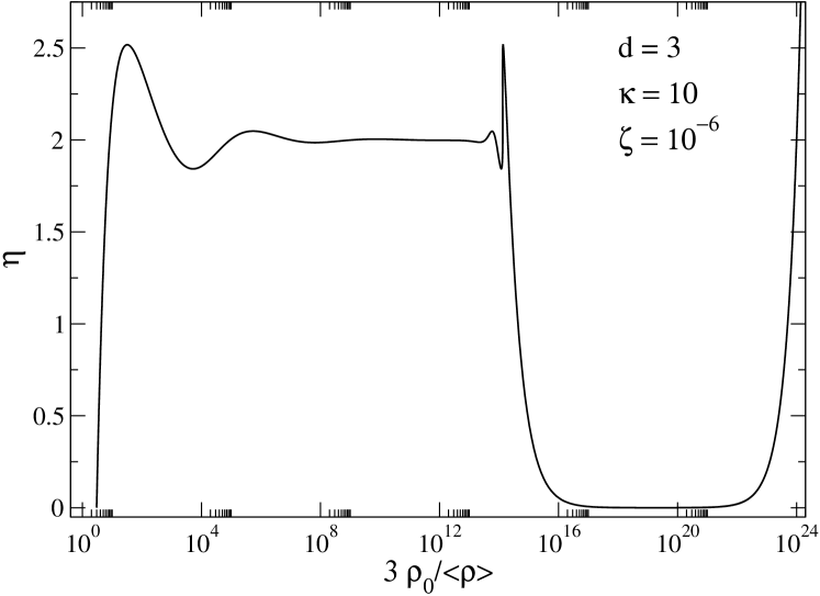
(a)    (b)

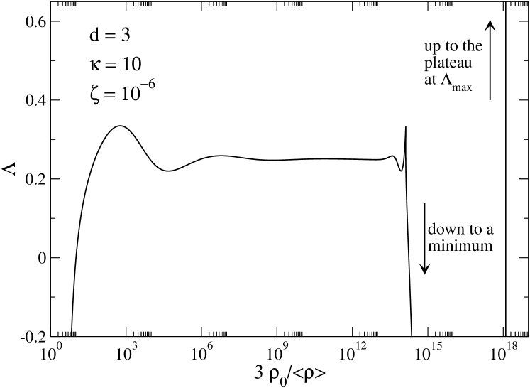
Figure 18: Evolution of the energy $\Lambda$ and inverse temperature $\eta$ as a function of the normalized central density $\rho_{0}/\langle{\rho}\rangle$.

III.7 Critical points

The deformation of the series of equilibria as a function of the core radius $R_{*}$ (for a fixed density $\rho_{*}$ of the central body) is represented in Figs. 19 and 20. There are two critical points in the problem, one in each ensemble. When $R_{*}<R_{*}^{\rm MCP}$, the series of equilibria $\beta(E)$ presents turning points of energy and temperature so that there exist phase transitions in the microcanonical and canonical ensembles. We have seen that the first order phase transitions may not take place in practice due to the long lifetime of the metastable states. However, there remains zeroth order phase transitions associated with the gravothermal catastrophe in the microcanonical ensemble and the isothermal collapse in the canonical ensemble. Since the domains of stability differ in the canonical and microcanonical ensembles, the ensembles are not equivalent. Indeed, some states are stable (i.e., accessible) in the microcanonical ensemble while they are unstable (i.e., inaccessible) in the canonical ensemble. Since canonical stability implies microcanonical stability cc , the microcanonical ensemble contains more stable states than the canonical one. At the microcanonical critical point $R_{*}=R_{*}^{\rm MCP}$, the series of equilibria $\beta(E)$ presents an inflexion point so that the microcanonical phase transition (gravothermal catastrophe) is suppressed (see Fig. 19). When $R_{*}^{\rm MCP}<R_{*}<R_{*}^{\rm CCP}$, the series of equilibria $\beta(E)$ presents turning points of temperature but no turning point of energy. Therefore, there exist phase transitions in the canonical ensemble but not in the microcanonical ensemble. The ensembles are not equivalent as revealed by the region of negative specific heat in the microcanonical ensemble that is replaced by a phase transition in the canonical ensemble. At the canonical critical point $R_{*}=R_{*}^{\rm CCP}$, the series of equilibria $E(\beta)$ presents an inflexion point so that the canonical phase transition (isothermal collapse) is suppressed (see Fig. 20). When $R_{*}>R_{*}^{\rm CCP}$, the series of equilibria $\beta(E)$ is monotonic so that there is no phase transition. In that case, the statistical ensembles are equivalent.

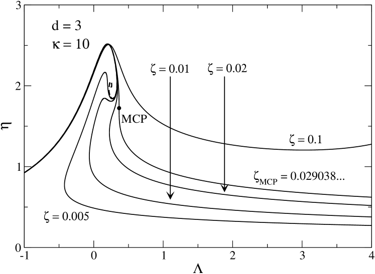
Figure 19: Enlargement of the series of equilibria near the microcanonical critical point. When $\zeta=\zeta_{\rm MCP}$, the curve $\eta(\Lambda)$ presents an inflexion point and the microcanonical phase transition (gravothermal catastrophe) is suppressed.

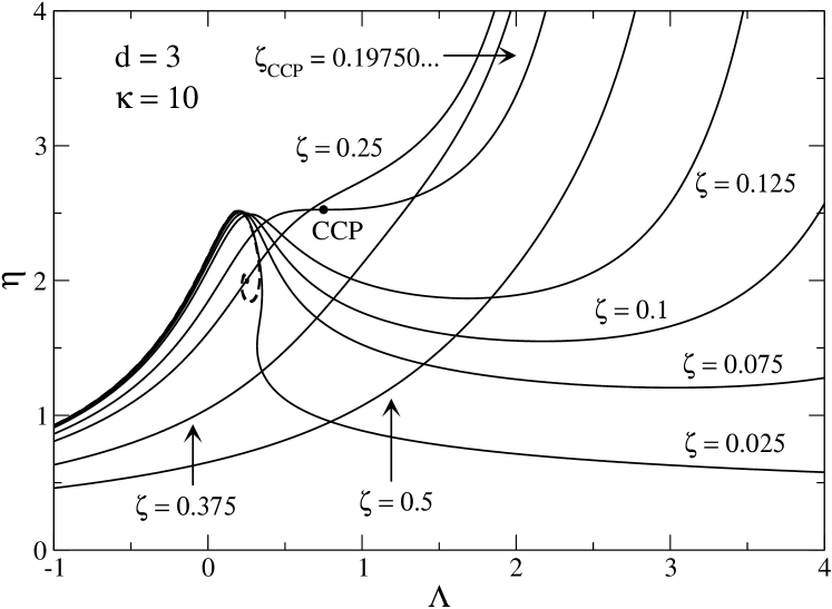
Figure 20: Enlargement of the series of equilibria near the canonical critical point. When $\zeta=\zeta_{\rm CCP}$, the curve $\Lambda(\eta)$ presents an inflexion point and the canonical phase transition (isothermal collapse) is suppressed.

The values of the microcanonical and canonical critical points $R_{*}^{\rm MCP}(\rho_{*})$ and $R_{*}^{\rm CCP}(\rho_{*})$ depend on the density $\rho_{*}$ of the central body. This dependence is represented in Fig. 21. At sufficiently large densities, the critical radii $R_{*}^{\rm MCP}(\rho_{*})$ and $R_{*}^{\rm CCP}(\rho_{*})$ decrease algebraically as $\rho_{*}^{-\alpha}$ with an exponent $\alpha\sim 0.3$.

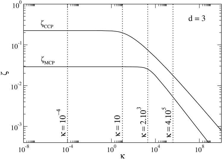
Figure 21: Dependence of the microcanonical and canonical critical points $\zeta_{\rm MCP}$ and $\zeta_{\rm CCP}$ with the density of the central body $\kappa$. We have indicated for reference the values of $\kappa$ that have been selected to construct the phase diagrams of Sec. III.8 (see Figs. 22 and 23 below).

III.8 Canonical and microcanonical phase diagram

Typical curves illustrating canonical and microcanonical phase transitions are represented in Figs. 11 and 6 respectively. The phase diagrams of an isothermal gas with a central body can be directly obtained from these curves by identifying characteristic energies and characteristic temperatures.

In the canonical ensemble (see Fig. 11), where $T$ is the control parameter, we note $T_{c}$ (collapse temperature) the terminal point of the metastable gaseous phase (first turning point of temperature), and $T_{*}$ (temperature of explosion) the terminal point of the metastable condensed phase (last turning point of temperature). These are the canonical spinodal points. The canonical phase diagram $(R_{*},T)$ is represented in Fig. 22 for different values of the density $\rho_{*}$ of the central body. For $T>T_{*}$, the system is in the gaseous phase and for $T<T_{c}$ the system is in the condensed phase. For $T_{*}<T<T_{c}$ it can be in one of these two phases (as a stable or a metastable state) depending on the way it has been prepared. This is the region where hysteretic effects take place. The two characteristic temperatures $T_{c}$ and $T_{*}$ merge at the canonical critical point $R_{*}=R_{*}^{\rm CCP}$. The strict phase diagram should exhibit the transition temperature $T_{t}$ corresponding to the first order phase transition (see ijmpb for self-gravitating fermions). However, since this phase transition does not take place in practice, we have only represented the physical phase diagram.

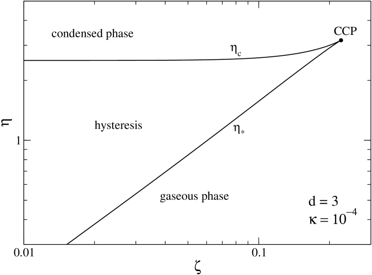
(a)    (b)

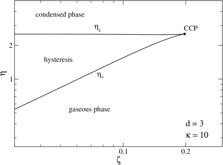
(c)

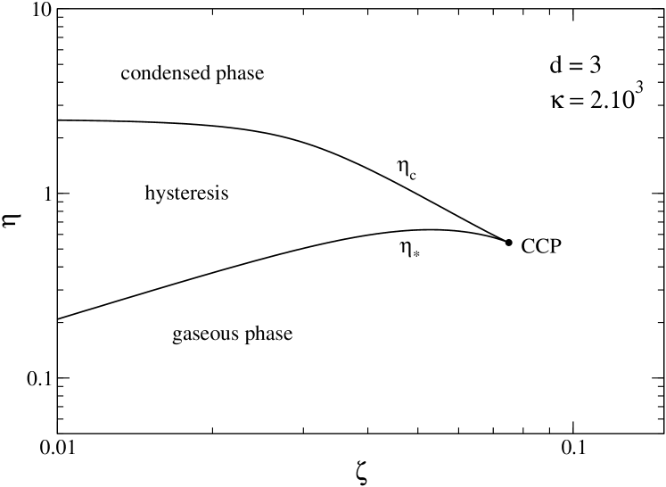
Figure 22: Canonical phase diagrams in the $(\zeta,\eta)$ plane for different values of the parameter $\kappa$ indicated in Fig. 21 (the canonical phase diagram for $\kappa=4\times 10^{5}$ is similar to the one for $\kappa=2\times 10^{3}$ so it is not represented). The region delimited by $\eta_{c}$ and $\eta_{*}$ corresponds to an hysteretic zone where the actual phase of the system depends on its history. If the system is initially prepared in a gaseous state, it will remain gaseous until the minimum temperature $1/\eta_{c}$, at which it will collapse and become condensed. Inversely, if the system is initially prepared in a condensed state, it will remain condensed until the maximum temperature $1/\eta_{*}$, at which it will explode and become gaseous.

In the microcanonical ensemble (see Fig. 6), where $E$ is the control parameter, we note $E_{c}$ (collapse energy) the end point of the metastable gaseous phase (first turning point of energy), and $E_{*}$ (energy of explosion) the end point of the metastable condensed phase (last turning point of energy). These are the microcanonical spinodal points. We also note $E_{\rm min}$ the minimum energy. The microcanonical phase diagram $(R_{*},E)$ is represented in Fig. 23 for different values of the density $\rho_{*}$ of the central body. For $E>E_{*}$, the system is in the gaseous phase and for $E_{\rm min}<E<E_{c}$ the system is in the condensed phase. For $E_{*}<E<E_{c}$ it can be in one of these two phases (as a stable or a metastable state) depending on the way it has been prepared. This is the region where hysteretic effects take place. The two characteristic energies $E_{c}$ and $E_{*}$ merge at the microcanonical critical point $R_{*}=R_{*}^{\rm MCP}$. To complete the diagram, we have also denoted $E_{\rm gas}$ the energy at which we enter in the region of negative specific heats (first turning point of temperature) and $E_{\rm cond}$ the energy at which we leave the region of negative specific heats (last turning point of temperature), see Fig. 10. These two characteristic energies $E_{\rm gas}$ and $E_{\rm cond}$ merge at the canonical critical point $R_{*}=R_{*}^{\rm CCP}$. The strict phase diagram should exhibit the transition energy $E_{t}$ corresponding to the first order phase transition (see ijmpb for self-gravitating fermions). However, since this phase transition does not take place in practice, we have only represented the physical phase diagram.

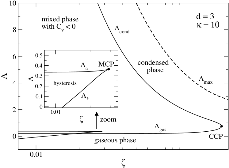
(a)    (b)

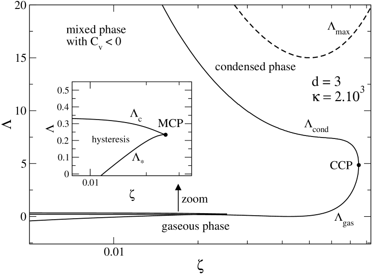
(c)

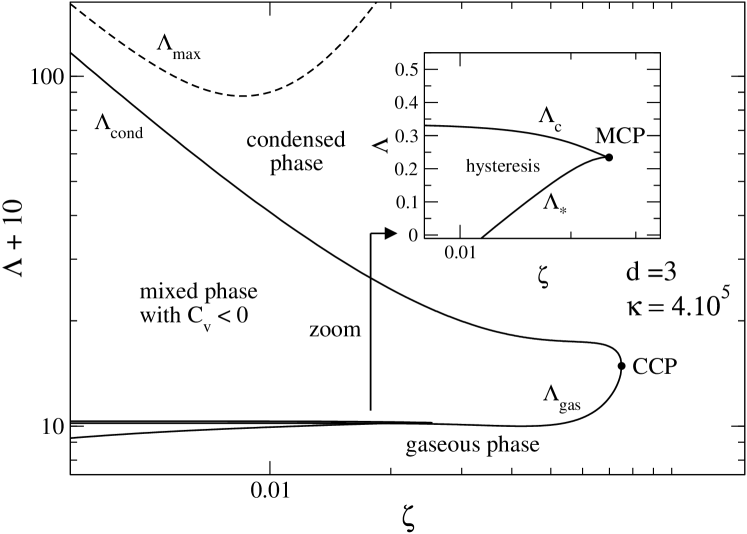
Figure 23: Microcanonical phase diagrams in the $(\zeta,\Lambda)$ plane for different values of the parameter $\kappa$ indicated in Fig. 21 (the microcanonical phase diagram for $\kappa=10^{-4}$ is similar to the one for $\kappa=10$ so it is not represented). The region delimited by $\Lambda_{c}$ and $\Lambda_{*}$ corresponds to an hysteretic zone where the actual phase of the system depends on its history. If the system is initially prepared in a gaseous state, it will remain gaseous until the minimum energy $-\Lambda_{c}$, at which it will collapse and become condensed. Inversely, if the system is initially prepared in a condensed state, it will remain condensed until the maximum energy $-\Lambda_{*}$, at which it will explode and become gaseous.

We note that the microcanonical phase diagram is richer than the canonical phase diagram due to the existence of a negative specific heat region. We recall that canonical stability implies microcanonical stability but the converse is false in case of ensemble inequivalence cc . Therefore, canonical stability is a sufficient but not necessary condition of microcanonical stability. Since canonical equilibria are always realized as microcanonical equilibria, they constitute a sub-domain of the microcanonical phase diagram. In particular, the states with energy between $E_{\rm gas}$ and $E_{\rm cond}$, that have negative specific heats, are not accessible in the canonical ensemble (they are unstable saddle points of free energy) while they are accessible in the microcanonical ensemble (they are entropy maxima at fixed mass and energy). Therefore, this region corresponds to a domain of ensemble inequivalence.

III.9 The case of a denser and denser central body and the case of a central Dirac mass

We consider how the series of equilibria changes when the radius of the central body $R_{*}$ is fixed and its mass $M_{*}$ is progressively increased so that the density $\rho_{*}$ of the central body is larger and larger. The series of equilibria are represented in Fig. 24. As the density $\rho_{*}$ increases, the collapse temperature $T_{c}$ and the collapse energy $E_{c}$ increase, so that instability occurs sooner. Typical density profiles at the verge of the canonical instability ($T=T_{c}$) are represented in Fig. 25. The cusp is more and more pronounced as the density of the central body increases.

Finally, we consider the case where the mass $M_{*}$ of the central body is fixed and its radius $R_{*}$ is progressively reduced. The corresponding caloric curves are plotted in Fig. 26. For $R_{*}\rightarrow 0$, the central body tends to a Dirac mass. However, we know from Sec. II.7 that there is no equilibrium state in that case in $d=3$. This is why the caloric curves do not tend to a well-defined limit for $R_{*}\rightarrow 0$.

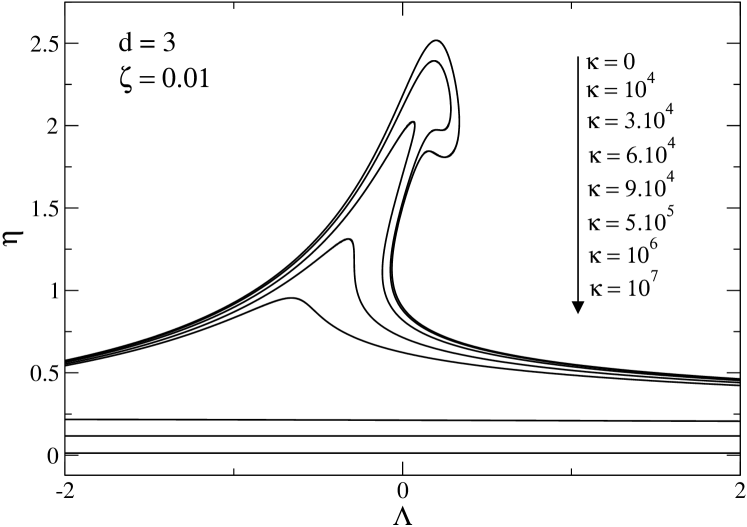
Figure 24: Deformation of the series of equilibria as we progressively increase the density $\kappa$ of the central body for a fixed value of the core radius $\zeta=0.01$.

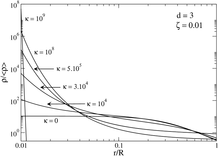
Figure 25: Density profiles corresponding to the critical temperature $\eta=\eta_{c}$ as one increases the density of the central body. As $\kappa$ increases, the self-gravitating particles are more and more condensed around the central body.

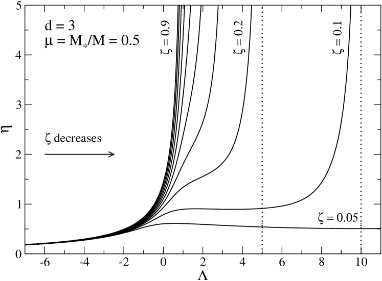
Figure 26: Caloric curves at fixed central mass $\mu$ (we have taken $\mu=0.5$ for illustration) for several values of the central body radius $\zeta$. The case $\zeta\rightarrow 0$ corresponds to a central Dirac mass for which there is no equilibrium state.

IV Caloric curves in the presence of a central body in $d=2$ and $d=1$ dimensions

In this section, we briefly describe the caloric curves of a classical isothermal self-gravitating gas in the presence of a central body in $d=2$ and $d=1$ dimensions. These caloric curves and the corresponding density profiles can be obtained analytically companion . In the figures, we fix the mass $M_{*}$ of the central body and decrease its radius $R_{*}$, approaching thereby a central Dirac mass when $R_{*}\rightarrow 0$.

We consider only box-confined systems and refer to companion for complementary results.

The caloric curve of a classical self-gravitating gas without central body in $d=2$ dimensions has been discussed by Katz and Lynden-Bell klb and Sire and Chavanis sc . The caloric curve $\beta(E)$ is monotonic (which implies thermodynamical stability) but the temperature tends to a constant $k_{B}T_{c}=GMm/4$ when $E\rightarrow-\infty$. Stable equilibrium state exists for all energies $E$ in the microcanonical ensemble, but only for temperatures $T>T_{c}$ in the canonical ensemble. For $T\leq T_{c}$ the system collapses and ultimately forms a Dirac peak containing all the mass sc . In the presence of a central body, the caloric curve is plotted in Fig. 27. There is a minimum energy $E_{\rm min}$ at which the gas is concentrated on the surface of the solid body (see Appendix F). A stable equilibrium state exists for all energies $E\geq E_{\rm min}$ in the microcanonical ensemble and for all temperatures $T\geq 0$ in the canonical ensemble. As $R_{*}$ decreases, the minimum energy $E_{\rm min}$ is pushed towards more and more negative values and a plateau forms at a critical temperature $k_{B}T_{c}=(GMm/4)(1+2{M_{*}}/{M})$ modified by the presence of the central Dirac mass $M_{*}$ companion . These results are similar to those obtained for a Fermi gas in $d=2$ dimensions ptd ; exclusion ; kmcfermions .

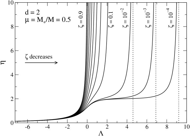
Figure 27: Caloric curves at fixed central mass $\mu$ (we have taken $\mu=0.5$ for illustration) for several values of the central body radius $\zeta$. For small $\zeta$ (corresponding to a central Dirac mass), one observes the appearance of the critical temperature $\eta_{c}=4/(1+2\mu)=2$.

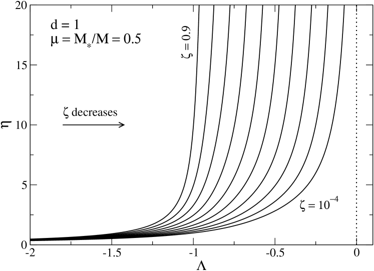
Figure 28: Caloric curves at fixed central mass $\mu$ (we have taken $\mu=0.5$ for illustration) for several values of the central body radius $\zeta$. For small $\zeta$ (corresponding to a central Dirac mass), the minimum energy approaches the absolute minimum value $\Lambda=0$.

The caloric curve of a classical self-gravitating gas without central body in $d=1$ dimension has been discussed by Katz and Lecar kl and Sire and Chavanis sc . The caloric curve $\beta(E)$ is monotonic (which implies thermodynamical stability). Stable equilibrium state exists for all accessible energies $E\geq 0$ in the microcanonical ensemble, and for all temperatures $T\geq 0$ in the canonical ensemble. There are no mechanical instabilities. In the presence of a central body, the caloric curve is plotted in Fig. 28. There is a minimum energy $E_{\rm min}>0$ at which the gas is concentrated on the surface of the solid body (see Appendix F). A stable equilibrium state exists for all energies $E\geq E_{\rm min}$ in the microcanonical ensemble, and for all temperatures $T\geq 0$ in the canonical ensemble. As $R_{*}$ decreases, the minimum energy is pushed towards $E=0$. These results are similar to those obtained for a Fermi gas in $d=1$ ptd ; exclusion ; kmcfermions .

V Conclusion

In this work, we have studied the statistical equilibrium states of a classical self-gravitating gas around a central body. The central body can represent a planetary core or mimic a black hole at the center of a galaxy or at the center of a globular cluster. The gas is described by the Boltzmann distribution which is the fundamental distribution function predicted by statistical mechanics. Like in previous studies, we must enclose the system within a box in order to have a well-defined equilibrium (maximum entropy state). Otherwise the gas evaporates and there is no statistical equilibrium state in a strict sense.

We have studied the phase transitions of this system in both microcanonical (fixed energy) and canonical (fixed temperature) ensembles in different dimensions of space. In $d=3$ dimensions, and for sufficiently large systems, we have evidenced both microcanonical and canonical phase transitions. Below a critical energy in the microcanonical ensemble the atmosphere experiences a gravothermal catastrophe and below a critical temperature in the canonical ensemble it experiences an isothermal collapse. In the presence of a central body, the collapse stops when the gas comes into contact with the central body and forms a thin layer (spike) around it. This leads to a zeroth order phase transition between a dilute (gaseous) phase and a condensed phase with a “cusp-halo” structure. For intermediate-size systems, there are only canonical phase transitions (of zeroth order) and for small systems there is no phase transition at all. In $d=2$ dimensions, there is no phase transition in a strict sense (no discontinuity of any thermodynamical parameter) but, for sufficiently large systems, a plateau temperature indicates a rapid change between a dilute phase and a condensed phase. In $d=1$ dimension, there is no phase transition. In $d=3$ dimensions there are regions of ensemble inequivalence (except for small systems) associated with negative specific heats while in $d=2$ and $d=1$ dimensions the specific heat is positive and the ensembles are equivalent. These results are similar to those obtained previously for self-gravitating fermions ijmpb . There is, however, a structural difference. In the case of fermions, the small-scale regularization is intrinsic to the quantum system (it arises from the Pauli exclusion principle contained in the Fermi-Dirac distribution) while, in the present case, the distribution function is classical and the small-scale regularization is external to the system (it is due to the finite radius of the central body).

Of course, the box is artificial and we can have two points of view on this problem. If we are mainly interested in statistical mechanics, it is relevant to use the Boltzmann distribution (which is the fundamental distribution function of statistical mechanics) and introduce a box to make the problem well-defined mathematically. In this sense, our thermodynamic approach is rigorously justified. If we are rather interested in astrophysical applications, we can use a truncated Boltzmann distribution, e.g., the King king distribution, to take into account the evaporation of the particles and avoid the artificial box. Although we gain in realism, the problem becomes less well-justified from a statistical mechanics point of view because we now have to deal with an out-of-equilibrium problem. We can nevertheless try to apply a thermodynamical approach as discussed by Katz katzking and Chavanis et al. clm1 for the classical King model. The study of phase transitions in the fermionic King model stella ; chavmnras has been performed in clm2 ; adky both for nonrelativistic and relativistic systems, giving results qualitatively similar to those obtained in a box ijmpb ; calettre ; acepjb . Recently, Bonsor et al. bonsor have considered the equilibrium states of a loaded King distribution around a central body. In this study, the central body models a black hole at the center of a globular cluster. They report a transition between equilibria which are dominated by the mass of the host stellar system or by the mass of the central black hole. Their results are complementary to those obtained for the classical and fermionic King models studied in clm1 ; clm2 and for the box-confined classical isothermal gas surrounding a central body considered in the present article. These works provide a rather complete picture of gravitational phase transitions in these different contexts.

Appendix A Analogy between self-gravitating systems and bacterial populations

In this Appendix, we point out some analogies between a gas of self-gravitating Brownian particles crs ; sc ; post and the chemotaxis of bacterial populations murray (see, e.g., crrs ; cskin ; chemocoll ; kss ; cd for more details on this analogy). The name chemotaxis refers to the motion of organisms induced by chemical signals. In some cases, the biological organisms secrete a substance (chemoattractant, pheromone) that has an attractive effect on the organisms themselves. Therefore, in addition to their diffusive motion, they move systematically along the gradient of concentration of the chemical they secrete (chemotactic flux). When attraction prevails over diffusion, the chemotaxis can trigger a self-accelerating process (chemotactic collapse) until a point at which aggregation takes place. This is the case for the slime mold Dictyostelium discoideum and for the bacteria Escherichia coli. The Keller-Segel ks model describing the chemotaxis of biological populations can be written as

$$\frac{\partial\rho}{\partial t}=\nabla\cdot(D\nabla\rho-\chi\rho\nabla c),$$ (92)

$$\frac{1}{D^{\prime}}\frac{\partial c}{\partial t}=\Delta c-k^{2}c+\lambda\rho,$$ (93)

where $\rho({\bf r},t)$ is the concentration of the biological species (e.g., bacteria) and $c({\bf r},t)$ is the concentration of the secreted chemical. The bacteria diffuse with a diffusion coefficient $D$ and undergo a chemotactic drift with strength $\chi$ along the gradient of chemical. The chemical is produced by the bacteria at a rate $D^{\prime}\lambda$, is degraded at a rate $D^{\prime}k^{2}$, and diffuses with a diffusion coefficient $D^{\prime}$. In the limit of large diffusivity of the chemical $D^{\prime}\rightarrow+\infty$ and a vanishing degradation rate $k^{2}=0$, the reaction-diffusion equation (93) reduces to the Poisson equation $\Delta c=-\lambda\rho$ (see Appendix C of cskin for more details). In that case, the Keller-Segel model becomes isomorphic to the Smoluchowski-Poisson equations describing self-gravitating Brownian particles in a high friction limit $\xi\rightarrow+\infty$ crs ; sc ; post :

$$\xi\frac{\partial\rho}{\partial t}=\nabla\cdot\left(\frac{k_{B}T}{m}\nabla\rho+\rho\nabla\Phi\right),$$ (94)

$$\Delta\Phi=S_{d}G\rho.$$ (95)

In this analogy, the concentration of chemical $c({\bf r},t)$, plays the role of minus the gravitational potential $-\Phi({\bf r},t)$. The effective statistical ensemble associated with the Keller-Segel model is the canonical ensemble. The steady states of the Keller-Segel model are of the form $\rho=Ae^{(\chi/D)c}$ which is similar to the Boltzmann distribution $\rho=Ae^{-\beta m\Phi}$ with an effective temperature $T_{\rm eff}=D/\chi$ given by a form of Einstein relation. The Lyapunov functional associated with the Keller-Segel model is $F=-\frac{1}{2}\int\rho c\,d{\bf r}+\frac{D}{\chi}\int\rho\ln\rho\,d{\bf r}$. It is similar to a free energy $F=E-TS$ in thermodynamics, where $E$ is the energy and $S$ is the Boltzmann entropy. The Keller-Segel model conserves the mass and satisfies an $H$-theorem for the free energy, i.e., $\dot{F}\leq 0$ with an equality if, and only if, $\rho$ is the Boltzmann distribution discussed above. Furthermore, the Boltzmann distribution is dynamically stable if, and only if, it is a local minimum of free energy at fixed mass. In that context, the minimization problem $\min_{\rho}\{F[\rho]|M[\rho]=M\}$ determines a steady state of the Keller-Segel model that is dynamically stable. This is similar to a condition of thermodynamical stability in the canonical ensemble.

Appendix B The virial theorem

In this Appendix we derive the equilibrium scalar virial theorem for a self-gravitating system in the presence of a central body in $d$ dimensions. We refer to Appendix G of ggpp and Appendix B of ggppbh for more details and generalizations.

B.1 The virial of the gravitational force produced by the central body

Assuming that the central body is spherically symmetric, and using Newton’s law (see Appendix D), the gravitational field that it creates in $r\geq R_{*}$ is

$$-\nabla\Phi_{\rm ext}=-\frac{GM_{*}}{r^{d-1}}{\bf e}_{r}\quad{\rm or}\quad\frac{d\Phi_{\rm ext}}{dr}=\frac{GM_{*}}{r^{d-1}}.$$ (96)

In particular, we have

$$\frac{d\Phi_{\rm ext}}{dr}(R_{*})=\frac{GM_{*}}{R_{*}^{d-1}}.$$ (97)

The corresponding gravitational potential in $r\geq R_{*}$ is

$$\Phi_{\rm ext}=-\frac{1}{d-2}\frac{GM_{*}}{r^{d-2}}\quad(d\neq 2),$$ (98)

$$\Phi_{\rm ext}=GM_{*}\ln\left(\frac{r}{R}\right)\quad(d=2).$$ (99)

This is the solution of the Laplace equation

$$\Delta\Phi_{\rm ext}=0.$$ (100)

The gravitational energy of the gas in the potential created by the central body is

$$W_{\rm ext}=\int\rho\Phi_{\rm ext}\,d{\bf r}.$$ (101)

Using Eqs. (98) and (99) we get

$$W_{\rm ext}=-\frac{1}{d-2}\int\rho\frac{GM_{*}}{r^{d-2}}\,d{\bf r}\quad(d\neq 2),$$ (102)

$$W_{\rm ext}=GM_{*}\int\rho\ln\left(\frac{r}{R}\right)\,d{\bf r}\quad(d\neq 2).$$ (103)

The virial of the external force is defined by

$$W^{\rm ext}_{ii}=-\int\rho{\bf r}\cdot\nabla\Phi_{\rm ext}\,d{\bf r}.$$ (104)

Using Eq. (96), we get

$$W^{\rm ext}_{ii}=-\int\rho\frac{GM_{*}}{r^{d-2}}\,d{\bf r}.$$ (105)

For $d\neq 2$, comparing Eqs. (102) and (105) we find that

$$W^{\rm ext}_{ii}=(d-2)W_{\rm ext}.$$ (106)

For $d=2$, Eq. (105) yields

$$W^{\rm ext}_{ii}=-GM_{*}M.$$ (107)

B.2 The virial of the gravitational force produced by the gas

The gravitational field produced by the gas is

$$-\nabla\Phi({\bf r})=-G\int\rho({\bf r}^{\prime})\frac{{\bf r}-{\bf r}^{\prime}}{|{\bf r}-{\bf r}^{\prime}|^{d}}\,d{\bf r}^{\prime}.$$ (108)

The corresponding gravitational potential is

$$\Phi({\bf r})=-\frac{G}{d-2}\int\frac{\rho({\bf r}^{\prime})}{|{\bf r}-{\bf r}^{\prime}|^{d-2}}\,d{\bf r}^{\prime}\qquad(d\neq 2),$$ (109)

$$\Phi({\bf r})=G\int\rho({\bf r}^{\prime})\ln\frac{|{\bf r}-{\bf r}^{\prime}|}{R}\,d{\bf r}^{\prime}\qquad(d=2).$$ (110)

This is the solution of the Poisson equation

$$\Delta\Phi=S_{d}G\rho.$$ (111)

The gravitational energy of the gas due to the interaction of the particles between themselves is

$$W=\frac{1}{2}\int\rho\Phi\,d{\bf r}.$$ (112)

Using Eqs. (109) and (110) we get

$$W=-\frac{1}{2}\frac{G}{d-2}\int\frac{\rho({\bf r})\rho({\bf r}^{\prime})}{|{\bf r}-{\bf r}^{\prime}|^{d-2}}\,d{\bf r}d{\bf r}^{\prime}\qquad(d\neq 2),$$ (113)

$$W=\frac{1}{2}G\int{\rho({\bf r})\rho({\bf r}^{\prime})}\ln\frac{|{\bf r}-{\bf r}^{\prime}|}{R}\,d{\bf r}d{\bf r}^{\prime}\qquad(d=2).$$ (114)

The virial of the gravitational force produced by the gas is

$$W_{ii}=-\int\rho{\bf r}\cdot\nabla\Phi\,d{\bf r}.$$ (115)

Substituting Eq. (108) into Eq. (115), we get

$$W_{ii}=-G\int\rho({\bf r})\rho({\bf r}^{\prime})\frac{{\bf r}\cdot({\bf r}-{\bf r}^{\prime})}{|{\bf r}-{\bf r}^{\prime}|^{d}}\,d{\bf r}d{\bf r}^{\prime}.$$ (116)

Interchanging the dummy variables ${\bf r}$ and ${\bf r}^{\prime}$ and adding the resulting expression to Eq. (116), we obtain

$$W_{ii}=-\frac{1}{2}G\int\frac{\rho({\bf r})\rho({\bf r}^{\prime})}{|{\bf r}-{\bf r}^{\prime}|^{d-2}}\,d{\bf r}d{\bf r}^{\prime}.$$ (117)

For $d\neq 2$, comparing Eqs. (113) and (117) we find that

$$W_{ii}=(d-2)W.$$ (118)

For $d=2$, Eq. (117) yields

$$W_{ii}=-\frac{GM^{2}}{2}.$$ (119)

These results are valid for an arbitrary distribution of the particles of the gas. In particular, for $d\neq 2$, we have

$$W=-\frac{1}{d-2}\int\rho{\bf r}\cdot\nabla\Phi\,d{\bf r}.$$ (120)

Now, for a spherically symmetric system, according to Newton’s law (see Appendix D), we have

$$-\nabla\Phi=-\frac{GM(r)}{r^{d-1}}{\bf e}_{r}\quad{\rm or}\quad\frac{d\Phi}{dr}=\frac{GM(r)}{r^{d-1}},$$ (121)

where

$$M(r)=\int_{R_{*}}^{r}\rho(r^{\prime})S_{d}{r^{\prime}}^{d-1}\,dr^{\prime}$$ (122)

is the mass of the gas contained within the sphere of radius $r$. Using Eq. (121) or Eq. (120), the virial of the gravitational force (115) can be written as

$$W_{ii}=-S_{d}G\int_{R_{*}}^{R}\rho(r)M(r)r\,dr=-\int_{R_{*}}^{R}\frac{GM(r)}{r^{d-2}}\,dM(r).$$ (123)

For $d=2$, we immediately recover Eq. (119). For $d\neq 2$, using Eq. (118), we obtain the formula

$$W=-\frac{1}{d-2}\int_{R_{*}}^{R}\rho(r)\frac{GM(r)}{r^{d-2}}S_{d}r^{d-1}\,dr,$$ (124)

which is useful to calculate the gravitational potential energy of a spherically symmetric distribution of matter. This expression can be directly obtained by approaching from infinity a succession of spherical shells of mass $dM(r)=\rho(r)S_{d}r^{d-1}dr$ with potential energy $-GM(r)dM(r)/[(d-2)r^{d-2}]$ in the field of the mass $M(r)$ already present, and integrating over $r$.

Remark: Combining Eqs. (59), (102) and (124) we get

$$W_{\rm tot}=-\frac{1}{d-2}\int_{R_{*}}^{R}\rho(r)\frac{G(M_{*}+M(r))}{r^{d-2}}S_{d}r^{d-1}\,dr$$ (125)

or, equivalently,

$$W=-\frac{S_{d}G}{d-2}\int_{R_{*}}^{R}\rho(r)(M_{*}+M(r))r\,dr.$$ (126)

B.3 The equilibrium virial theorem

The condition of hydrostatic equilibrium from Eq. (43) can be rewritten as

$$\nabla P+\rho\nabla\Phi+\rho\nabla\Phi_{\rm ext}={\bf 0}.$$ (127)

Taking the scalar product of this relation with ${\bf r}$ and integrating over the region containing the gas we get

$$\int{\bf r}\cdot\nabla P\,d{\bf r}-W_{ii}-W^{\rm ext}_{ii}=0,$$ (128)

where $W^{\rm ext}_{ii}$ and $W_{ii}$ are defined by Eqs. (104) and (115). Integrating by parts, we obtain the scalar virial theorem

$$d\int P\,d{\bf r}+W_{ii}+W^{\rm ext}_{ii}=\oint P{\bf r}\cdot d{\bf S}.$$ (129)

For a nonrelativistic gas, the local pressure is given by

$$P=\frac{1}{d}\int fv^{2}\,d{\bf v}.$$ (130)

This relation is valid for an arbitrary distribution function. The kinetic energy is

$$E_{\rm kin}=\int f\frac{v^{2}}{2}\,d{\bf r}d{\bf v}.$$ (131)

Therefore, we have the relation

$$E_{\rm kin}=\frac{d}{2}\int P\,d{\bf r}.$$ (132)

The scalar virial theorem can then be rewritten as

$$2E_{\rm kin}+W_{ii}+W^{\rm ext}_{ii}=\oint P{\bf r}\cdot d{\bf S}.$$ (133)

For $d\neq 2$, using Eqs. (106) and (118) we obtain

$$2E_{\rm kin}+(d-2)W_{\rm tot}=\oint P{\bf r}\cdot d{\bf S},$$ (134)

where we have introduced $W_{\rm tot}=W+W_{\rm ext}$. For $d=2$, using Eqs. (107) and (119) we get

$$2E_{\rm kin}-\frac{GM^{2}}{2}\left(1+2\frac{M_{*}}{M}\right)=\oint P{\bf r}\cdot d{\bf S}.$$ (135)

To obtain these identities, we have not assumed that the gas is spherically symmetric (only that the central body is spherically symmetric). Now, for a spherically symmetric system enclosed between the spheres of radius $R_{*}$ and $R$, owing to the fact that the pressure $P$ is uniform on these spheres, we have

$$\oint P{\bf r}\cdot d{\bf S}=d(P(R)V-P(R_{*})V_{*}),$$ (136)

where $V$ and $V_{*}$ are the volumes of the spheres of radius $R$ and $R_{*}$ respectively. Since $V=\frac{1}{d}S_{d}R^{d}$ this relation can be rewritten as

$$\oint P{\bf r}\cdot d{\bf S}=P(R)S_{d}R^{d}-P(R_{*})S_{d}R_{*}^{d}.$$ (137)

The scalar virial theorem is then given by Eqs. (134) and (135) with Eq. (137).

Appendix C Condition of hydrostatic equilibrium for a spherical and isotropic stellar system

Let us consider a stellar system described by a distribution function $f({\bf r},{\bf v})$. For a spherical and isotropic system we have $f=f(\epsilon)$ where $\epsilon=v^{2}/2+\Phi({\bf r})$ is the individual energy of the stars by unit of mass. We define the density

$$\rho({\bf r})=\int f\,d{\bf v}=\int f[v^{2}/2+\Phi({\bf r})]\,d{\bf v}$$ (138)

and the pressure

$$P({\bf r})=\frac{1}{d}\int fv^{2}\,d{\bf v}=\frac{1}{d}\int f[v^{2}/2+\Phi({\bf r})]v^{2}\,d{\bf v}.$$ (139)

We note that $\rho({\bf r})=\rho[\Phi({\bf r})]$ and $P({\bf r})=P[\Phi({\bf r})]$ depend only on the gravitational potential. Eliminating formally $\Phi({\bf r})$ between these two expressions, we find that the equation of state is barotropic in the sense that the pressure depends only on the density: $P({\bf r})=P[\rho({\bf r})]$. We can therefore associate to the stellar system with distribution function $f(\epsilon)$ a corresponding barotropic gas with an equation of state $P=P(\rho)$. Taking the gradient of the pressure in Eq. (139) and making straightforward manipulations, we get

$$\nabla P = \frac{1}{d}\nabla\Phi\int f^{\prime}(\epsilon)v^{2}\,d{\bf v}$$ (140)

$$= \frac{1}{d}\nabla\Phi\int\frac{\partial f}{\partial{\bf v}}\cdot{\bf v}\,d{\bf v}$$

$$= -\frac{1}{d}\nabla\Phi\int f\nabla\cdot{\bf v}\,d{\bf v}$$

$$= -\nabla\Phi\int f\,d{\bf v}.$$

We therefore recover the condition of hydrostatic equilibrium for a gas

$$\nabla P+\rho\nabla\Phi={\bf 0}.$$ (141)

In the presence of an external potential $\Phi_{\rm ext}$, we just have to make the substitution $\Phi\rightarrow\Phi+\Phi_{\rm ext}$.

Appendix D Newton’s law in $d$ dimensions

If we consider a spherically symmetric distribution of matter with density $\rho(r)$, the Poisson equation

$$\Delta\Phi=S_{d}G\rho$$ (142)

becomes

$$\frac{1}{r^{d-1}}\frac{d}{dr}\left(r^{d-1}\frac{d\Phi}{dr}\right)=S_{d}G\rho.$$ (143)

Integrating this equation between $0$ and $r$, we obtain

$$\frac{d\Phi}{dr}=\frac{GM(r)}{r^{d-1}},$$ (144)

where

$$M(r)=\int_{0}^{r}\rho(r^{\prime})S_{d}{r^{\prime}}^{d-1}\,dr^{\prime}$$ (145)

denotes the mass contained within the sphere of radius $r$. We have

$$\rho(r)=\frac{M^{\prime}(r)}{S_{d}r^{d-1}}.$$ (146)

Eq. (144) expresses Newton’s second theorem (in $d$ dimensions) saying that the gravitational force produced in $r$ by a spherically symmetric distribution of matter is the same as it would be if all the mass $M(r)$ were concentrated into a point at its center. In vectorial form,

$$-\nabla\Phi=-\frac{GM(r)}{r^{d-1}}{\bf e}_{r}.$$ (147)

This equation can also be obtained by integrating Eq. (142) over a sphere of radius $r$ and using the Gauss (or Ostrogradsky) theorem.

If the density $\rho(r)$ vanishes above a certain radius $R$, then for $r\geq R$, we have

$$\frac{d\Phi}{dr}=\frac{GM}{r^{d-1}},$$ (148)

where $M=M(R)$ is the mass enclosed within the sphere of radius $R$. In particular, we obtain

$$\frac{d\Phi}{dr}(R)=\frac{GM}{R^{d-1}}.$$ (149)

For $r\geq R$, the gravitational potential is given by

$$\Phi(r)=-\frac{1}{d-2}\frac{GM}{r^{d-2}}\quad(d\neq 2),$$ (150)

$$\Phi(r)=GM\ln\left(\frac{r}{R}\right)\quad(d=2).$$ (151)

In particular,

$$\Phi(R)=-\frac{1}{d-2}\frac{GM}{R^{d-2}}\quad(d\neq 2),$$ (152)

$$\Phi(R)=0\quad(d=2).$$ (153)

Appendix E The potential in $d=3$ dimensions for a spherically symmetric system

For a spherically symmetric system, the gravitational potential in $d=3$ can be written as

$$\Phi({r})=-G\int_{R_{*}}^{R}\int_{0}^{2\pi}\int_{0}^{\pi}\frac{\rho({r}_{1})}{|{\bf r}-{\bf r}_{1}|}\sin\theta\,d\theta d\phi r_{1}^{2}d{r}_{1}.$$ (154)

Introducing the expansion

$$\frac{1}{|{\bf r}-{\bf r}_{1}|}=\sum_{l=0}^{+\infty}\frac{r_{<}^{l}}{r_{>}^{l+1}}P_{l}(\cos\theta),$$ (155)

where $r_{<}={\rm min}(r,r_{1})$ and $r_{>}={\rm max}(r,r_{1})$ in Eq. (154), making the change of variable $x=\cos\theta$ and using the identity $\int_{-1}^{+1}P_{l}(x)dx=2\delta_{l0}$, we find that

$$\Phi({r})=-4\pi G\left[\frac{1}{r}\int_{R_{*}}^{r}\rho(r_{1})r_{1}^{2}dr_{1}+\int_{r}^{R}\rho(r_{1})r_{1}dr_{1}\right].$$

From this expression, we get

$$\Phi(R_{*})=-4\pi G\int_{R_{*}}^{R}\rho(r)rdr.$$ (157)

Appendix F The energy of the ground state

At $T=0$, all the gas is uniformly concentrated on the surface of the central body. Therefore, the energy of the ground state $E_{\rm min}=W_{\rm tot}^{\rm min}$ corresponds to the potential energy associated to this configuration. To compute this minimum energy, we start from Eq. (59). Accounting for the fact that the total mass of the gas $M$ is located at $r=R_{*}$, we have

$$E_{\rm min}=\frac{1}{2}M\Phi(R_{*})+\Phi_{\rm ext}(R_{*})M.$$ (158)

For $d\neq 2$, using Eqs. (98) and (150), we obtain

$$E_{\rm min}=-\frac{1}{d-2}(1+2\mu)\frac{GM^{2}}{R_{*}^{d-2}}.$$ (159)

The normalized minimum energy is therefore

$$\Lambda_{\rm max}=\frac{1+2\mu}{2(d-2)\zeta^{d-2}}.$$ (160)

For $d=2$, using Eqs. (99) and (151), we obtain

$$E_{\rm min}=\frac{GM^{2}}{2}(1+2\mu)\ln\left(\frac{R_{*}}{R}\right).$$ (161)

The normalized minimum energy is therefore

$$\Lambda_{\rm max}=-\frac{1}{2}(1+2\mu)\ln\zeta.$$ (162)

References

- (1) T. Padmanabhan, Phys. Rep. 188, 287 (1990)
- (2) H.J. de Vega, N. Sanchez, Nucl. Phys. B 625, 409 (2002)
- (3) H.J. de Vega, N. Sanchez, Nucl. Phys. B 625, 460 (2002)
- (4) J. Katz, Found. Phys. 33, 223 (2003)
- (5) P.H. Chavanis, Int. J. Mod. Phys. B 20, 3113 (2006)
- (6) Dynamics and thermodynamics of systems with long range interactions, edited by Dauxois, T., Ruffo, S., Arimondo, E., Wilkens, M. Lecture Notes in Physics, Springer (2002).
- (7) A. Campa, T. Dauxois, S. Ruffo, Physics Reports 480, 57 (2009)
- (8) A. Campa, T. Dauxois, D. Fanelli, S. Ruffo, Physics of long-range interacting systems (Oxford University Press, 2014)
- (9) V.A. Antonov, Vest. Leningr. Gos. Univ. 7, 135 (1962).
- (10) V.A. Ambarzumian, Ann. Leningrad State University 22, 19 (1938)
- (11) L. Spitzer, Mon. Not. R. Astron. Soc. 100, 396 (1940)
- (12) S. Chandrasekhar, Principles of Stellar Dynamics (University of Chicago press, 1942)
- (13) K.F. Ogorodnikov, Sov. Astron. 1, 748 (1957)
- (14) K.F. Ogorodnikov, Sov. Astron. 1, 787 (1957)
- (15) D. Lynden-Bell, R. Wood, Mon. Not. R. Astron. Soc. 138, 495 (1968).
- (16) D. Lynden-Bell, Extrait du Bulletin Astronomique 3, 305 (1968)
- (17) M. Hénon, Ann. Astrophys. 24, 369 (1961)
- (18) H. Cohn, Astrophys. J. 242, 765 (1980)
- (19) R.B. Larson, Mon. Not. R. Astron. Soc. 147, 323 (1970)
- (20) I. Hachisu, Y. Nakada, K. Nomoto, D. Sugimoto, Prog. Theor. Phys. 60, 393 (1978)
- (21) D. Lynden-Bell, P.P. Eggleton, Mon. Not. R. Astron. Soc. 191, 483 (1980)
- (22) S. Inagaki, D. Lynden-Bell, Mon. Not. R. Astron. Soc. 205, 913 (1983)
- (23) D.C. Heggie, D. Stevenson, Mon. Not. R. Astron. Soc. 230, 223 (1988)
- (24) D. Sugimoto, E. Bettwieser, Mon. Not. R. Astron. Soc. 204, 19 (1983)
- (25) P.H. Chavanis, Astron. Astrophys. 432, 117 (2005)
- (26) J. Binney, S. Tremaine Galactic Dynamics, Princeton Series in Astrophysics (1987)
- (27) R.W. Michie, Mon. Not. R. Astron. Soc. 125, 127 (1963)
- (28) I.R. King, Astron. J. 70, 376 (1965)
- (29) J. Katz, Mon. Not. R. Astron. Soc. 190, 497 (1980)
- (30) P.H. Chavanis, M. Lemou, F. Méhats, Phys. Rev. D 91, 063531 (2015)
- (31) W. Thirring, Z. Phys. 235, 339 (1970).
- (32) D. Lynden-Bell, R.M. Lynden-Bell, Mon. Not. R. Astron. Soc. 181, 405 (1977)
- (33) R. Emden, Gaskugeln (Teubner Verlag, Leipzig, 1907).
- (34) P.H. Chavanis, Astron. Astrophys. 381, 340 (2002)
- (35) M. Kiessling, J. Stat. Phys. 55, 203 (1989)
- (36) P.H. Chavanis, C. Rosier, C. Sire, Phys. Rev. E 66, 036105 (2002).
- (37) C. Sire, P.H. Chavanis, Phys. Rev. E 66, 046133 (2002).
- (38) C. Sire, P.H. Chavanis, Phys. Rev. E 69, 066109 (2004).
- (39) P.H. Chavanis, Astron. Astrophys. 356, 1089 (2000)
- (40) J. Katz, Mon. Not. R. Astron. Soc. 183, 765 (1978)
- (41) H. Poincaré, Acta Math. 7, 259 (1885)
- (42) E.B. Aronson, C.J. Hansen, Astrophys. J. 177, 145 (1972)
- (43) B. Stahl, M.K.H. Kiessling, K. Schindler Planet. Space Sci. 43, 271 (1994)
- (44) S. Chandrasekhar, An Introduction to the Theory of Stellar Structure (Dover, New York, 1942).
- (45) J.R. Oppenheimer, G.M. Volkoff, Phys. Rev. 55, 374 (1939)
- (46) S.L. Shapiro, S.A. Teukolsky Black Holes, White Dwarfs, and Neutron Stars (Wiley Interscience, 1983)
- (47) N. Bilic, F. Munyaneza, G.B. Tupper, R.D. Viollier, Prog. Part. Nucl. Phys. 48, 291 (2002)
- (48) N. Bilic, G.B. Tupper, R.D. Viollier, Lect. Notes Phys. 616, 24 (2003)
- (49) H.J. de Vega, P. Salucci, N.G. Sanchez, Mon. Not. R. Astron. Soc. 442, 2717 (2014)
- (50) R. Ruffini, C.R. Argüelles, J.A. Rueda, Mon. Not. R. Astron. Soc. 451, 622 (2015)
- (51) P.H. Chavanis, The self-gravitating Fermi gas in Newtonian gravity and general relativity, Proceedings of the Sixteenth Marcel Grossman Meeting (July, 2021) [arXiv:2112.02654]
- (52) P.H. Chavanis, Phys. Rev. D 106, 043538 (2022)
- (53) C.R. Argüelles, E.A. Becerra-Vergara, J.A. Rueda, R. Ruffini, Universe 9, 197 (2023)
- (54) P.H. Chavanis, Eur. Phys. J. B 87, 9 (2014)
- (55) B. Bakhti, D. Boukari, M. Karbach, P. Maass, G. Müller, Phys. Rev. E 97, 042131 (2018)
- (56) P. Hertel and W. Thirring, Commun. Math. Phys. 24, 22 (1971)
- (57) P. Hertel, W. Thirring, in Quanten und Felder, ed. H.P. Dürr (Vieweg, Braunschweig, 1971).
- (58) N. Bilic, R.D. Viollier, Phys. Lett. B 408, 75 (1997)
- (59) P.H. Chavanis, Phys. Rev. E 65, 056123 (2002)
- (60) B. Miller, P. Youngkins, Phys. Rev. Lett. 81, 4794 (1998)
- (61) E. Follana, V. Laliena, Phys. Rev. E 61, 6270 (2000)
- (62) P. Youngkins, B. Miller, Phys. Rev. E 62, 4583 (2000)
- (63) P.H. Chavanis, I. Ispolatov, Phys. Rev. E 66, 036109 (2002)
- (64) C. Destri, H.J. de Vega, Nucl. Phys. B 763, 309 (2007)
- (65) N. Bilic, R.D. Viollier, Eur. Phys. J. C 11, 173 (1999)
- (66) Z. Roupas, P.H. Chavanis, Class. Quantum Grav. 36, 065001 (2019)
- (67) P.H. Chavanis, G. Alberti, Phys. Lett. B 801, 135155 (2020)
- (68) G. Alberti, P.H. Chavanis, Eur. Phys. J. B 93, 208 (2020)
- (69) P.H. Chavanis, M. Lemou, F. Méhats, Phys. Rev. D 92, 123527 (2015)
- (70) C. Argüelles, M.I. Díaz, A. Krut, R. Yunis, Mon. Not. R. Astron. Soc. 502, 4227 (2021)
- (71) J.D. Murray, Mathematical Biology (Springer, Berlin, 1991).
- (72) P.H. Chavanis, M. Ribot, C. Rosier, C. Sire, Banach Center Publ. 66, 103 (2004).
- (73) J.S. Stodolkiewicz, Acta Astr. 13, 30 (1963)
- (74) J. Ostriker, Astrophys. J. 140, 1056 (1964)
- (75) L. Spitzer, Astrophys. J. 95, 329 (1942)
- (76) G.L. Camm, Mon. Not. R. Astron. Soc. 110, 305 (1950)
- (77) P.H. Chavanis, Physica A 384, 392 (2007)
- (78) P.H. Chavanis, Phys. Rev. E 69, 066126 (2004)
- (79) P.H. Chavanis, Phys. Rev. D 76, 023004 (2007)
- (80) M. Kirejczyk, G. Müller, P.H. Chavanis, Phys. Rev. E 106, 024132 (2022)
- (81) M. Kirejczyk, G. Müller, P.H. Chavanis, Phys. Rev. E 105, 034145 (2022)
- (82) P.H. Chavanis, in preparation
- (83) P.H. Chavanis, Astron. Astrophys. 556, A93 (2013)
- (84) K.F. Ogorodnikov, Dynamics of Stellar Systems (Pergamon, 1965)
- (85) R. Ellis, K. Haven, B. Turkington, J. Stat. Phys. 101, 999 (2000)
- (86) A. Campa, P.H. Chavanis, J. Stat. Mech. 06, 06001 (2010)
- (87) P.H. Chavanis, J. Sommeria, Mon. Not. R. Astron. Soc. 296, 569 (1998)
- (88) I. Ispolatov, M. Karttunen, Phys. Rev. E 68, 036117 (2003)
- (89) J. Katz, D. Lynden-Bell, Mon. Not. R. Astron. Soc. 184, 709 (1978)
- (90) J. Katz, M. Lecar, Astr. Space. Sci. 68, 495 (1980)
- (91) R. Ruffini, L. Stella, Astron. Astrophys. 119, 35 (1983)
- (92) P.H. Chavanis, Mon. Not. R. Astron. Soc. 300, 981 (1998)
- (93) S.R. Bonsor, A.L. Varri, J. Vanneste, preprint
- (94) P.H. Chavanis, C. Sire, Physica A 384, 199 (2007)
- (95) P.H. Chavanis, C. Sire, Physica A 387, 4033 (2008)
- (96) P.H. Chavanis, Commun. Nonlinear Sci. Numer. Simulat. 15 60 (2010)
- (97) P.H. Chavanis, L. Delfini, Phys. Rev. E 89, 032139 (2014).
- (98) E. Keller, L.A. Segel, J. Theor. Biol. 26, 399 (1970).
- (99) P.H. Chavanis, Eur. Phys. J. Plus 132, 248 (2017)
- (100) P.H. Chavanis, Eur. Phys. J. Plus 134, 352 (2019)