SurvBeX: An explanation method of the machine learning survival models based on the Beran estimator

Abstract

An explanation method called SurvBeX is proposed to interpret predictions of the machine learning survival black-box models. The main idea behind the method is to use the modified Beran estimator as the surrogate explanation model. Coefficients, incorporated into Beran estimator, can be regarded as values of the feature impacts on the black-box model prediction. Following the well-known LIME method, many points are generated in a local area around an example of interest. For every generated example, the survival function of the black-box model is computed, and the survival function of the surrogate model (the Beran estimator) is constructed as a function of the explanation coefficients. In order to find the explanation coefficients, it is proposed to minimize the mean distance between the survival functions of the black-box model and the Beran estimator produced by the generated examples. Many numerical experiments with synthetic and real survival data demonstrate the SurvBeX efficiency and compare the method with the well-known method SurvLIME. The method is also compared with the method SurvSHAP. The code implementing SurvBeX is available at: https://github.com/DanilaEremenko/SurvBeX

Keywords: interpretable model, explainable AI, LIME, survival analysis, censored data, the Beran estimator, the Cox model.

1 Introduction

Censored survival data can be met in many applications, including medicine, the system reliability and safety, economics [1, 2]. They consider times to an event of interest as observations. The event might not have happened during the period of study [3]. If the observed survival time is less than or equal to the true survival time, then the corresponding data is censored and called right-censoring data. Machine learning models dealing the survival data are based on applying the framework and concepts of survival analysis and conditionally divided into parametric, nonparametric and semiparametric models [2].

There are different methods for constituting machine learning survival models. We consider models which depend on the feature vectors characterizing objects, whose times to an event are studied, for example, patients, the system structures, Many survival models are based on using the Cox proportional hazard method or the Cox model [4], which calculates effects of observed covariates on the risk of an event occurring under condition that a linear combination of the instance covariates is assumed in the model. The success of the Cox model in many applied tasks motivated to generalize the model in order to consider non-linear functions of covariates or several regularization constraints for the model parameters [5, 6, 7, 8]. To improve survival analysis and to enhance the prediction accuracy of the machine learning survival models, other approaches have been developed, including the SVM approach [9], random survival forests (RSF) [10, 11, 12, 13, 14], survival neural networks [5, 6, 15, 8].

The most survival models can be regarded as black-box models because details of their functioning are often completely unknown, but their inputs as well as outcomes may be known for users. As a results, it is difficult to explain how a prediction corresponding to a certain input is achieved, which features of the input significantly impact on the prediction. However, the explanation of predictions should be an important component of intelligent systems especially in medicine [16] where a doctor has to understand why the used machine learning diagnostic model states a diagnosis. At present, there are many methods which can explain predictions of black-box models ‘[17, 18, 19, 20]. According to these methods, the explanation means to assign numbers to features, which quantify the feature impacts on the prediction. The methods can be divided into local and global explanation methods. Local methods produce explanation locally around an explained example whereas global methods explain the black-box model for the whole dataset.

An important local explanation method is the Local Interpretable Model-agnostic Explanations (LIME) [21], which explains predictions of a black-box model approximating a model function at a point by the linear model where coefficients of the linear model can be regarded as the quantified representation of the feature impacts on the prediction [22]. According to LIME, the linear model is constructed by generating randomly synthetic examples around the explained example. It should be noted that the idea to approximate the black-box model function at a point by the linear surrogate model is fruitful and can be applied to many classification and regression tasks.

In most applications, LIME deals with point-valued predictions. However, predictions of the survival machine learning models are functions, for example, the survival function (SF), the cumulative hazard function (CHF). In other words, explanation methods should explain which features have the significant impact on the form of the SF corresponding to some input object. To take into account peculiarities of the survival models, a series of the LIME modifications dealing with survival data and models and called SurvLIME have been presented in [23, 24, 25]. The main idea behind the SurvLIME is to approximate the black-box model at a point by the Cox model which is based on the linear combination of covariates. Coefficients of the linear combination can be viewed as measures of the covariate impact on the prediction in the form of the SF or the CHF.

Many numerical experiments have shown that the proposed SurvLIME models provide satisfactory results. However, limitations of the Cox model motivated to search for a more adequate model which could improve the explanation of survival models. One of the interesting model is the Beran estimator [26] which can be regarded as a kernel regression for computing the SF taking into account the data structure. However, the original Beran estimator does not contain linear combinations of covariates, which are needed to develop the linear approximation like the Cox model. Therefore, we proposed to modify the Beran estimator by incorporating a vector whose elements can be viewed as the feature impacts on the prediction. The proposed explanation model using the modified Beran estimator is called SurvBeX (Survival Beran eXplanation). It is similar to SurvLIME, but, in contrast to SurvLIME, it has several specific elements which distinguish SurvBeX from SurvLIME. Moreover, SurvBeX is more flexible because it has many opportunities for modifications. For example, it can be studied with different kernels which are important elements of the Beran estimator.

Our contributions can be summarized as follows:

1. A new method for explaining predictions of machine learning survival models based on applying the modification of the Beran estimator is proposed.

2. An algorithm implementing the method based on solving an unconstrained optimization problem is proposed.

3. Various numerical experiments compare the method with the well-known survival explanation method called SurvLIME under condition of using different black-box survival models, including the Cox model, the RSF, and the Beran estimator. SurvBeX is also compared with a very interesting method based on the survival extension of the method SHAP [27, 28], which is called SurvSHAP(t) [29]. The corresponding code implementing the proposed method is publicly available at: https://github.com/DanilaEremenko/SurvBeX.

Numerical results show that SurvBeX provides outperforming results in comparison with SurvLIME and SurvSHAP(t).

The paper is organized as follows. Related work can be found in Section 2. A short description of basic concepts of survival analysis and the explanation methods, including the Cox model, the original Beran estimator, LIME, SurvLIME, is given in Section 3. A general idea of SurvBeX is provided in Section 4. The formal derivation of the optimization problem for implementing SurvBeX and its simplification can be found in Section 5. Numerical experiments with synthetic data are provided in Section 6. Similar numerical experiments with real data are given in Section 7. Concluding remarks are provided in Section 8.

2 Related work

Local explanation methods. Due to the importance of explaining and interpreting the machine learning model predictions, many local explanation methods have been developed and studied. First of all, we have to point out the original LIME [21] and its various modifications, including ALIME [30], NormLIME [31], DLIME [32], Anchor LIME [33], LIME-SUP [34], LIME-Aleph [35], GraphLIME [36], Rank-LIME [37], s-LIME [38].

Along with LIME, another method of local explanation, called SHAP [28], is also actively used. It is based on applying a game-theoretic approach for optimizing a regression loss function using Shapley values [27]. Due to the strong theoretical justification of SHAP, a lot of its modifications also have been proposed, for example, SHAP-E [39], SHAP-IQ [40], K-SHAP [41], MM-SHAP [42], Latent SHAP [43], X-SHAP [44], Random SHAP [45].

Another interesting class of explanation methods is based on using ideas behind the Generalized Additive Model (GAM) [46]. Following this mode, the explainable boosting machine was proposed in [47] and [48]. Another model based on GAM is the Neural Additive Model (NAM) was proposed in [49]. NAM can be viewed as a neural network implementation of GAM where the network consists of a linear combination of “small” neural subnetworks having single inputs corresponding to each feature, i.e. a single feature is fed to each subnetwork producing a shape function of a feature. Similar approaches using neural networks for implementing GAM and performing shape functions called GAMI-Net and the Adaptive Explainable Neural Networks (AxNNs) were proposed in [50] and [51], respectively,

Critical and comprehensive surveys devoted to the local explanation methods can be found in [52, 53, 54, 55, 56, 57, 18, 19, 20, 58].

Machine learning models in survival analysis. Many machine learning models have the survival extension, i.e. they are modified in order to deal with survival data or with censored data. A detailed review of survival models is presented in [2]. The survival machine learning models can be divided into three groups. The first group consists of models which are based on the well-known statistical models, including the Cox model, The Kaplan-Meier models, etc. Several models from the first group use the Nadaraya-Watson regression for estimating SFs and other concepts of survival analysis [59, 60, 61, 62, 63]. Kernel-based estimators of SFs in survival analysis are studied in [64]. The second group consists of models which mainly adapt the original machine learning models to survival data. These are the SVM approach [65], the random survival forests [10, 13, 14], survival neural networks [6, 15]. The third group is some combinations of the models from the first and the second groups. Examples of these models are modifications of the Cox model relaxing the linear relationship assumption accepted in the Cox model, including neural networks instead of the linear relationship [66, 5], the Lasso modifications [67, 68, 7].

Most aforementioned survival models can be viewed as black-box models whose predictions should be explained in many applications. This motivates to develop the explanation methods which deal with survival data.

Explanation methods in survival analysis. One of the problems encountered the local explanation in survival analysis is to explain the function-valued predictions instead of the point-valued predictions which are explained by many methods. In survival analysis, predictions are usually SFs or CHFs which are functions of time. A new approach to deal with function-valued predictions is SurvLIME [23, 24, 25]. Its modification and the corresponding software is called SurvLIMEpy [69]. An extension to SurvLIME called SurvNAM has been proposed in [70]. SurvNAM can be also viewed as an extension to NAM [49]. An extension of the NAM for survival analysis with EHR Data was presented in [71].

A novel, easily deployable approach, called EXplainable CEnsored Learning, to iteratively exploit critical variables in the framework of survival analysis was developed in [72]. The authors of this work aim to find critical features with long-term prognostic values. The explainable machine learning, which provides insights in breast cancer survival, is considered in [73]. An interesting extension of the SHAP to its application in survival analysis, called SurvSHAP(t) has been proposed in [29]. The authors of the work introduce the first time-dependent explanation for interpreting machine learning survival models. The important feature of the SurvSHAP(t) method is that it explains the predicted SF.

3 Elements of survival analysis

3.1 Basic concepts

An example (object) in survival analysis is usually represented by a triplet $(\mathbf{x}_{i},\delta_{i},T_{i})$, where $\mathbf{x}_{i}^{\mathrm{T}}=(x_{i1},...,x_{id})$ is the vector of the example features; $T_{i}$ is time to event of interest for the $i$-th example. If the event of interest is observed, then $T_{i}$ is the time between a baseline time and the time of event happening. In this case, an uncensored observation takes place and $\delta_{i}=1$. Another case is when the event of interest is not observed. Then $T_{i}$ is the time between the baseline time and the end of the observation. In this case, a censored observation takes place and $\delta_{i}=0$. There are different types of censored observations. We will consider only right-censoring, where the observed survival time is less than or equal to the true survival time [1]. Given a training set $\mathcal{A}$ consisting of $n$ triplets $(\mathbf{x}_{i},\delta_{i},T_{i})$, $i=1,...,n$, the goal of survival analysis is to estimate the time to the event of interest $T$ for a new example $\mathbf{x}$ by using $\mathcal{A}$.

Key concepts in survival analysis are SFs, hazard functions, and the CHF, which describe probability distributions of the event times. The SF denoted as $S(t|\mathbf{x})$ is the probability of surviving up to time $t$, that is $S(t|\mathbf{x})=\Pr\{T>t|\mathbf{x}\}$. The hazard function $h(t|\mathbf{x})$ is the rate of the event at time $t$ given that no event occurred before time $t$. The hazard function can be expressed through the SF as follows [1]:

$$h(t|\mathbf{x})=-\frac{\mathrm{d}}{\mathrm{d}t}\ln S(t|\mathbf{x}).$$ (1)

The CHF denoted as $H(t|\mathbf{x})$ is defined as the integral of the hazard function $h(t|\mathbf{x})$ and can be interpreted as the probability of the event at time $t$ given survival until time $t$, that is

$$H(t|\mathbf{x})=\int_{-\infty}^{t}h(z|\mathbf{x})dz.$$ (2)

An important relationship between the SF and the CHF is

$$S(t|\mathbf{x})=\exp\left(-H(t|\mathbf{x})\right).$$ (3)

To compare survival models, the C-index proposed by Harrell et al. [74] is used. It estimates how good a survival model is at ranking survival times. It estimates the probability that, in a randomly selected pair of examples, the example that fails first had a worst predicted outcome. In fact, this is the probability that the event times of a pair of examples are correctly ranking.

C-index has different forms. One of the forms is [75]:

$$C=\frac{\sum\nolimits_{i,j}\mathbf{1}[T_{i}<T_{j}]\cdot\mathbf{1}[\widehat{T}_{i}<\widehat{T}_{j}]\cdot\delta_{i}}{\sum\nolimits_{i,j}\mathbf{1}[T_{i}<T_{j}]\cdot\delta_{i}},$$

where $\widehat{T}_{i}$ and $\widehat{T}_{j}$ are the predicted survival durations.

3.2 The Cox model

The Cox proportional hazards model is used as an important component in SurvLIME. Therefore, we provide some details of the model. According to the Cox model, the hazard function at time $t$ given vector $\mathbf{x}$ is defined as [4, 1]:

$$h(t|\mathbf{x},\mathbf{b})=h_{0}(t)\exp\left(\mathbf{b}^{\mathrm{T}}\mathbf{x}\right).$$ (4)

Here $h_{0}(t)$ is a baseline hazard function which does not depend on the vector $\mathbf{x}$ and the vector $\mathbf{b}$; $\mathbf{b}^{\mathrm{T}}=(b_{1},...,b_{m})$ is an unknown vector of the regression coefficients or the model parameters. The baseline hazard function represents the hazard when all of the covariates are equal to zero.

The SF in the framework of the Cox model is

$$S(t|\mathbf{x},\mathbf{b})=\exp(-H_{0}(t)\exp\left(\mathbf{b}^{\mathrm{T}}\mathbf{x}\right))=\left(S_{0}(t)\right)^{\exp\left(\mathbf{b}^{\mathrm{T}}\mathbf{x}\right)}.$$ (5)

Here $H_{0}(t)$ is the baseline CHF; $S_{0}(t)$ is the baseline SF which is defined as the survival function for zero feature vector $\mathbf{x}^{\mathrm{T}}=(0,...,0)$. The baseline SF and CHF do not depend on $\mathbf{x}$ and $\mathbf{b}$.

One of the ways to compute the parameters $\mathbf{b}$ is to use the partial likelihood defined as follows [4]:

$$L(\mathbf{b})=\prod_{j=1}^{n}\left[\frac{\exp(\mathbf{b}^{\mathrm{T}}\mathbf{x}_{j})}{\sum_{i\in R_{j}}\exp(\mathbf{b}^{\mathrm{T}}\mathbf{x}_{i})}\right]^{\delta_{j}},$$ (6)

where $R_{j}$ is the set of objects which are at risk at time $t_{j}$. The term “at risk at time $t$” means objects for which the event of interest happens at time $t$ or later. Only uncensored observations are used in the likelihood function.

3.3 The Beran estimator

Given the dataset $\mathcal{A}$, the SF can be estimated by using the Beran estimator [26] as follows:

$$S_{B}(t|\mathbf{x},\mathcal{A})=\prod_{t_{i}\leq t}\left\{1-\frac{\alpha(\mathbf{x},\mathbf{x}_{i})}{1-\sum_{j=1}^{i-1}\alpha(\mathbf{x},\mathbf{x}_{j})}\right\}^{\delta_{i}},$$ (7)

where time moments are ordered; the weight $\alpha(\mathbf{x},\mathbf{x}_{i})$ conforms with relevance of the $i$-th example $\mathbf{x}_{i}$ to the vector $\mathbf{x}$ and can be defined through kernels as

$$\alpha(\mathbf{x},\mathbf{x}_{i})=\frac{K(\mathbf{x},\mathbf{x}_{i})}{\sum_{j=1}^{n}K(\mathbf{x},\mathbf{x}_{j})}.$$ (8)

If we use the Gaussian kernel, then the weights $\alpha(\mathbf{x},\mathbf{x}_{i})$ are of the form:

$$\alpha(\mathbf{x},\mathbf{x}_{i})=\text{{softmax}}\left(-\frac{\left\|\mathbf{x}-\mathbf{x}_{i}\right\|^{2}}{\tau}\right),$$ (9)

where $\tau$ is a tuning (temperature) parameter.

Below another representation of the Beran estimator will be used:

$$S_{B}(t|\mathbf{x},\mathcal{A})=\prod_{t_{i}\leq t}\left\{\frac{1-\sum_{j=1}^{i}\alpha(\mathbf{x},\mathbf{x}_{j})}{1-\sum_{j=1}^{i-1}\alpha(\mathbf{x},\mathbf{x}_{j})}\right\}^{\delta_{i}}.$$ (10)

The Beran estimator can be regarded as a generalization of the Kaplan-Meier estimator [2] because it is reduced to the Kaplan-Meier estimator if the weights $\alpha(\mathbf{x},\mathbf{x}_{i})$ take values $\alpha(\mathbf{x},\mathbf{x}_{i})=1/n$ for all $i=1,...,n$. The product in (7) takes into account only uncensored observations whereas the weights are normalized by using uncensored as well as censored observations.

3.4 LIME

LIME aims to approximate a black-box model implementing a function $q(\mathbf{x)}$ by a linear function $g(\mathbf{x)}$ in the vicinity of the explained point $\mathbf{x}$ [21]. Generally, the function $g(\mathbf{x)}$ may be arbitrary from a set $G$ of explainable functions. LIME proposes to perturb new examples and obtain the corresponding predictions for the examples by means of the black-box model. This set of the examples jointly with the predictions forms a dataset for learning the function $g(\mathbf{x)}$. To take into account different distances from $\mathbf{x}$ and the generated examples, weights $w_{\mathbf{x}}$ are assigned in accordance with the distances by using a kernel function.

An explanation (local surrogate) model is trained by solving the following optimization problem:

$$\arg\min_{g\in G}L(q,g,w_{\mathbf{x}})+\Phi(g).$$ (11)

Here $L$ is a loss function, for example, mean squared error (MSE), which measures how the explanation is close to the prediction of the black-box model; $\Phi(g)$ is the model complexity.

If $g(\mathbf{x)}$ is linear, then the corresponding prediction is explained by analyzing values of coefficients of $g(\mathbf{x)}$.

3.5 SurvLIME

SurvLIME is a modification of LIME when the black-box model is survival [23]. In contrast to the original LIME, SurvLIME approximates the black-box model with the Cox model.

Suppose there is a training set $\mathcal{A}$ and a black-box model. The model prediction is represented in the form of the CHF $H(t|\mathbf{x})$ for every new example $\mathbf{x}$. SurvLIME approximates the black-box model prediction by the Cox model prediction with the CHF $H_{\text{Cox}}(t|\mathbf{x},\mathbf{b})$. Values of parameters $\mathbf{b}$ can be regarded as quantitative impacts on the prediction $H(t|\mathbf{x})$. They are unknown and have to be found by means of the approximation of models. Optimal coefficients $\mathbf{b}$ make the distance between CHFs $H(t|\mathbf{x})$ and $H_{\text{Cox}}(t|\mathbf{x},\mathbf{b})$ for the example $\mathbf{x}$ as small as possible.

In order to implement the approximation at point $\mathbf{x}$, many nearest examples $\mathbf{x}_{k}$ are generated in a local area around $\mathbf{x}$. The CHF $H(t|\mathbf{x}_{k})$ predicted by the black-box model is computed for every generated $\mathbf{x}_{k}$. Optimal values of $\mathbf{b}$ can be found by minimizing the weighted average distance between every pair of CHFs $H(t|\mathbf{x}_{k})$ and $H_{\text{Cox}}(t|\mathbf{x}_{k},\mathbf{b})$ over all generated points $\mathbf{x}_{k}$. Weight $w_{k}$ depends on the distance between points $\mathbf{x}_{k}$ and $\mathbf{x}$. Smaller distances between $\mathbf{x}_{k}$ and $\mathbf{x}$ define larger weights of distances between CHFs. The distance metric between CHFs defines the corresponding optimization problem for computing optimal coefficients $\mathbf{b}$. Therefore, SurvLIME [23] uses the $l_{2}$-norm applied to logarithms of CHFs $H(t|\mathbf{x}_{k})$ and $H_{\text{Cox}}(t|\mathbf{x}_{k},\mathbf{b})$, which leads to a simple convex optimization problem with variables $\mathbf{b}$.

One of the limitations of SurvLIME is caused by the underlying Cox model: even in small neighborhoods in the feature space, the proportional hazards assumption may be violated, leading to an inaccurate surrogate model. Another limitation is the linear relationship of covariates in the Cox model, which may be a reason for the inadequate approximation of black-box models by SurvLIME. In order to overcome the aforementioned SurvLIME drawbacks, it is proposed to replace the Cox model by the Beran estimator for explaining predictions produced by a black-box. In other words, it is proposed to approximate the prediction of the black-box model by means of the Beran estimator.

4 A general idea of SurvBeX

Given a training set $\mathcal{A}$ and a black-box model which is explained, for every new example $\mathbf{x}$, the black-box model produces the corresponding output in the form of the SF $S(t|\mathbf{x})$. A general algorithm of SurvBeX is similar to SurvLIME. Suppose we have a new example $\mathbf{x}$ and the black-box produces a prediction in the form of SF $S(t|\mathbf{x})$. Let us incorporate parameters $\mathbf{b}=(b_{1},...,b_{d})$ into the Beran estimator (7) as follows:

$$\alpha(\mathbf{x},\mathbf{x}_{i},\mathbf{b})=\text{{softmax}}\left(-\frac{\left\|\mathbf{b}\odot\left(\mathbf{x}-\mathbf{x}_{i}\right)\right\|^{2}}{\tau}\right).$$ (12)

Here $\mathbf{b}\odot\mathbf{x}$ is the dot product of two vectors. It can be seen from the above that each element of $\mathbf{b}$ can be regarded as the quantitative impact of the corresponding feature on the prediction $S_{B}(t|\mathbf{x})$ which will be denoted as $S_{B}(t|\mathbf{x},\mathbf{b})$ to indicate the dependence of the SF on parameters $\mathbf{b}$. If we approximate the function $S(t|\mathbf{x})$ by the function $S_{B}(t|\mathbf{x},\mathbf{b})$, then coefficients $\mathbf{b}$ show which features in $\mathbf{x}$ are the most important. Actually, elements of $\mathbf{b}$ weigh the difference between features $x_{j}$ and $x_{ij}$ of vectors $\mathbf{x}$ and $\mathbf{x}_{i}$, respectively. However, it follows from the Beran estimator that the predicted SF $S_{B}(t|\mathbf{x})$ depends on differences of vectors $\mathbf{x}$ and $\mathbf{x}_{i}$, but not on the vector $\mathbf{x}$ itself. Therefore, we use the above representation for $\alpha(\mathbf{x},\mathbf{x}_{i},\mathbf{b})$ in (7).

The remaining part of the algorithm does not substantially differ from SurvLIME. Suppose that the black-box model has been trained on the dataset $\mathcal{A}$. In order to find vector $\mathbf{b}$ in accordance with LIME or SurvLIME, we generate $N$ points $\mathbf{z}_{1},...,\mathbf{z}_{N}$ in a local area around $\mathbf{x}$. Different notations for training and generated examples are used in order to distinguish the corresponding sets of data. In contrast to vectors $\mathbf{x}_{1},...,\mathbf{x}_{n}$ from $\mathcal{A}$, which train the black-box model and the Beran estimator, points $\mathbf{z}_{k}$ can be viewed as tested examples for the black-box model and for the Beran estimator. For every point $\mathbf{z}_{k}$, the SF $S(t|\mathbf{z}_{k})$ is determined as a prediction of the black-box model. The SF $S_{B}(t|\mathbf{z}_{k},\mathbf{b})$ is represented by using (7) as a function of the parameter vector $\mathbf{b}$ which is unknown at this stage. So, we obtain $N$ SFs $S(t|\mathbf{z}_{k})$ and the same number of SFs $S_{B}(t|\mathbf{z}_{k},\mathbf{b})$. It is important to note that the Beran estimator uses the training dataset $\mathcal{A}$ to make predictions for the generated points $\mathbf{z}_{k}$.

In order to approximate functions $S(t|\mathbf{z}_{k})$ and $S_{B}(t|\mathbf{z}_{k},\mathbf{b})$ and to compute the vector $\mathbf{b}$, we minimize the average distance between the functions over the vector $\mathbf{b}$. The solution to the optimization problem is the optimal vector $\mathbf{b}^{opt}$ which explains the prediction $S(t|\mathbf{x})$ corresponding to the example $\mathbf{x}$. At that, we additionaly assign weights $w_{1},...,w_{N}$ to examples $\mathbf{z}_{1},...,\mathbf{z}_{N}$ such that the weight $w_{k}$ is defined by the distance between vectors $\mathbf{z}_{k}$ and $\mathbf{x}$. Smaller distances between $\mathbf{z}_{k}$ and $\mathbf{x}$ produce larger weights of distances between SFs $S(t|\mathbf{z}_{k})$ and $S_{B}(t|\mathbf{z}_{k},\mathbf{b})$. Weights can be calculated by using the standard normalized kernel $K^{\ast}(\mathbf{z}_{k},\mathbf{x})$. It should distinguish kernels $K^{\ast}$ and $K$. The kernel $K^{\ast}$ is for computing weights of generated examples, but the kernel $K$ is for computing weights $\alpha(\mathbf{x},\mathbf{x}_{i},\mathbf{b})$ from the Beran estimator. Weights $w_{k}$ are defined in the same way as in LIME.

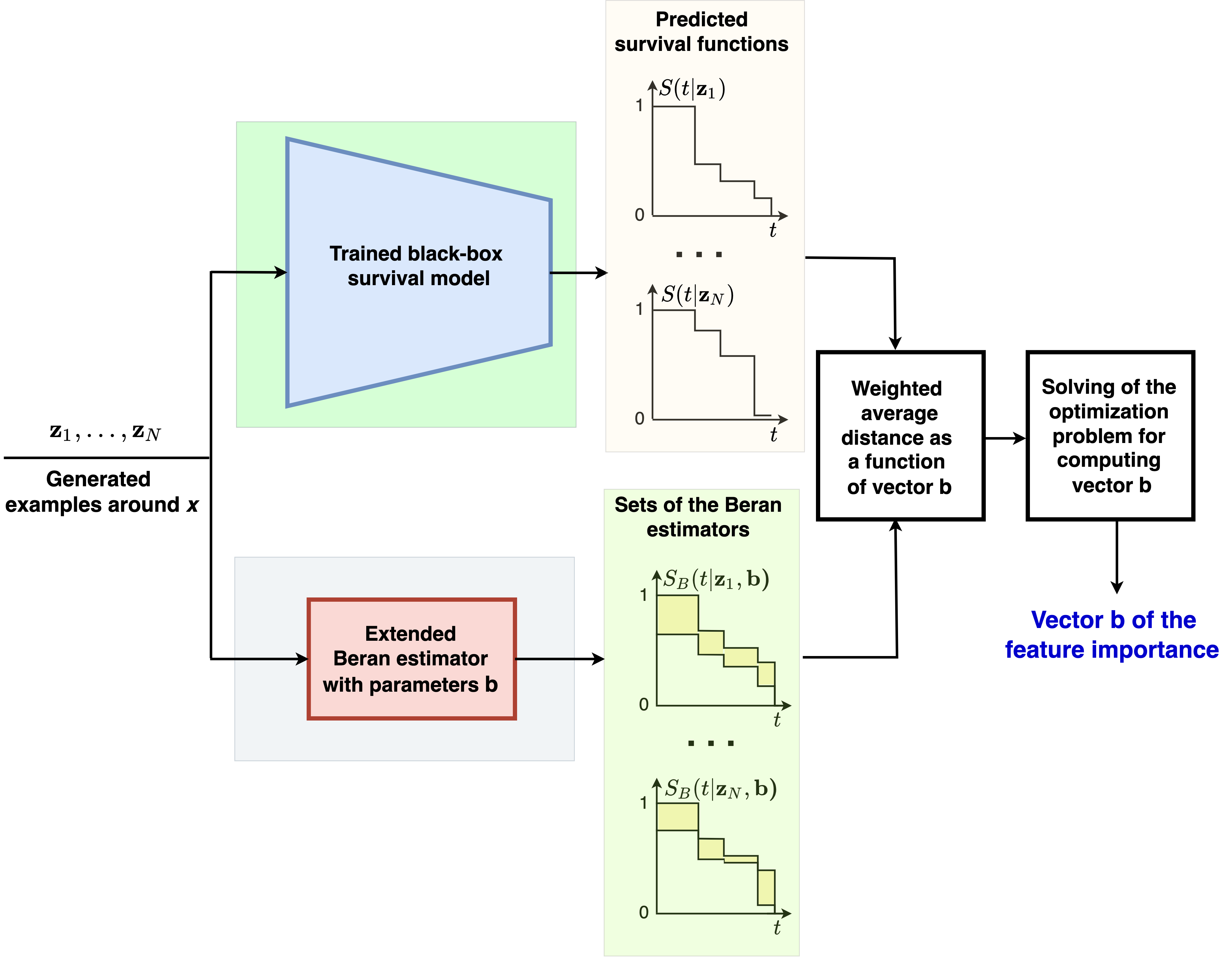
Figure 1: A general scheme of SurvBeX

A general scheme of SurvBeX is depicted in Fig. 1. It can be seen from Fig. 1 that two models (the trained black-box survival model and the extended Beran estimator with parameters $\mathbf{b}$) produce SFs corresponding to the generated points $\mathbf{z}_{1},...,\mathbf{z}_{N}$. Moreover, SFs produced by the Beran estimator can be regarded as a family of functions parametrized by $\mathbf{b}$. They are obtained in the implicit form as functions of $\mathbf{b}$. The objective function for computing $\mathbf{b}^{opt}$ is the weighted average distance between SFs $S(t|\mathbf{z}_{k})$ and $S_{B}(t|\mathbf{z}_{k},\mathbf{b})$.

Only an idea of SurvBeX is presented above. A formal description of the method which contains details of its implementation is provided in the next section.

5 Formal optimization problem statement

According to the general description of SurvBeX, $N$ examples are randomly generated with weights $w_{j}$ to construct an approximation of the predicted SF by the SF estimated by means of the Beran estimator at point $\mathbf{x}$. If we have the set $\mathcal{A}$ of $n$ training examples $(\mathbf{x}_{i},\delta_{i},T_{i})$ and the set of $N$ generated feature vectors $\mathbf{z}_{j}$ in a local area around the explained example $\mathbf{x}$, then the objective function of the optimization problem for computing optimal vector $\mathbf{b}$ is the weighted average distance between $N$ pairs of SFs $S(t|\mathbf{z}_{j})$ and $S_{B}(t|\mathbf{z}_{j},\mathbf{b})$, with weights $w_{j}$, $j=1,...,N$, which can be written as follows:

$$\min_{\mathbf{b}}\frac{1}{N}\sum_{j=1}^{N}w_{j}\cdot D\left(S(t|\mathbf{z}_{j}),S_{B}(t|\mathbf{z}_{j},\mathbf{b})\right).$$ (13)

Here $D\left(\cdot,\cdot\right)$ is a distance between two functions. Since many distance metrics are based on the norms $l_{s}$, $s=1,...,\infty$, then we can rewrite the optimization problem for these distance metrics

$$\min_{\mathbf{b}}\frac{1}{N}\sum_{j=1}^{N}w_{j}\left\|S(t|\mathbf{z}_{j})-S_{B}(t|\mathbf{z}_{j},\mathbf{b})\right\|_{s}^{s},$$ (14)

which in the case of finite $s$ is equivalent to

$$\min_{\mathbf{b}}\sum_{j=1}^{N}w_{j}\int_{0}^{\infty}\left|S(t|\mathbf{z}_{j})-S_{B}(t|\mathbf{z}_{j},\mathbf{b})\right|^{s}.$$ (15)

Let $t_{0}<t_{1}<...<t_{n}$ be ordered times to an event of interest from the set $\{T_{1},...,T_{n}\}$, where $t_{0}=0$ and $t_{n}=\max_{k=1,...,n}T_{k}$. It is assumed that all times are different. The times $t_{0},t_{1},...,t_{n}$ split the interval $\Omega=[t_{0},t_{n}]$ into $n$ non-intersecting subintervals $\Omega_{1},...,\Omega_{n}$ such that $\Omega_{k}=[t_{k-1},t_{k})$, $k=1,...,n$.

The black-box model maps the feature vectors $\mathbf{x}\in\mathbb{R}^{d}$ into piecewise constant SF $S(t|\mathbf{x})$ which can be represented as the sum

$$S(t|\mathbf{x})=\sum_{k=1}^{n}S^{(k)}(\mathbf{x})\cdot\chi_{\Omega_{k}}(t),$$ (16)

where $\chi_{\Omega_{k}}(t)$ is the indicator function taking value $1$ if $t\in\Omega_{k}$, and value $0$ if $t\notin\Omega_{k}$; $S^{(k)}(\mathbf{x})$ is the SF for $t\in\Omega_{k}$.

The same representation can be written for the SF $S_{B}(t|\mathbf{x},\mathbf{b})$ as well as for the difference of the SFs. We also assume that $S(t|\mathbf{x})=0$ for $t>t_{n}$. Then the objective function in the optimization problem for computing $\mathbf{b}$ can be formulated as

$$\sum_{j=1}^{N}w_{j}\int_{\Omega}\left|S(t|\mathbf{z}_{j})-S_{B}(t|\mathbf{z}_{j},\mathbf{b})\right|^{s}$$

$$=\sum_{j=1}^{N}w_{j}\sum_{i=1}^{n}\left|S^{(i)}(\mathbf{z}_{j})-S_{B}^{(i)}(\mathbf{z}_{j},\mathbf{b})\right|^{s}\left(t_{i}-t_{i-1}\right).$$ (17)

Similarly, we can state a problem to minimize the difference between logarithms of SFs in order to simplify the optimization problem. Let us introduce the condition $S^{(i)}(\mathbf{x})\geq\varepsilon>0$ for all $i=1,...,n$. Then the optimizatin problem can also be formulated through logarithms:

$$\mathbf{b}=\arg\min_{\mathbf{b}}\sum_{j=1}^{N}w_{j}\sum_{i=1}^{n}\left|\ln S^{(i)}(\mathbf{z}_{j})-\ln S_{B}^{(i)}(\mathbf{z}_{j},\mathbf{b})\right|^{s}\left(t_{i}-t_{i-1}\right),$$ (18)

where

$$\ln S_{B}^{(i)}(\mathbf{z}_{j},\mathbf{b})=\sum_{t_{l}\leq t_{i}}\delta_{l}\left[\ln\left(1-\sum_{k=1}^{l}\alpha(\mathbf{z}_{j},\mathbf{x}_{k})\right)-\ln\left(1-\sum_{k=1}^{l-1}\alpha(\mathbf{z}_{j},\mathbf{x}_{k})\right)\right].$$ (19)

The unconstrained optimization problem has been obtained, which can be solved by means of a gradient-based algorithm. The weight is defined as $w_{j}=K^{\ast}(\mathbf{x},\mathbf{z}_{j})$, where $K^{\ast}(\cdot,\cdot)$ is a kernel function which measures how similar two feature vectors. For example, if to use the Gaussian kernel, then the weight is defined as

$$w_{j}=\exp\left(-\left\|\mathbf{x}-\mathbf{z}_{j}\right\|^{2}/\sigma\right),$$ (20)

where $\sigma$ is the kernel parameter.

It should be noted that we use two different kernels. The first one is used for computing weights $\alpha(\mathbf{x},\mathbf{x}_{i})$ in the Beran estimator. The second kernel is used to find weights $w_{j}$ of the generated points in a local area around the explained example. The kernels also have different parameters.

Finally, we write Algorithm 1 implementing the proposed explanation method.

Algorithm 1 The algorithm implementing SurvBeX for computing vector $\bf{b}$ of the feature importance for point $\bf{x}$

0:  Training set $\mathcal{A}$; point of interest $\mathbf{x}$; the number of generated points $N$; parameters of kernels $\tau$ and $\sigma$.

0:  Vector $\mathbf{b}$ of important features of $\mathbf{x}$.

1:  Generate $N$ random points $\mathbf{z}_{k}$ in a local area around $\mathbf{x}$.

2:  Find predictions of SFs $S(t|\mathbf{z}_{j})$, $j=1,...,N$, produced by the black-box survival model.

3:  Compute weights $w_{j}=K^{\ast}(\mathbf{x},\mathbf{z}_{j})$ of generated points, $j=1,...,N$, by using (20).

4:  Construct the optimization problem (17) by using (19) and (7) with weights $\alpha(\mathbf{x},\mathbf{x}_{i},\mathbf{b})$ expressed through (12).

5:  Find vector $\mathbf{b}$ by solving the optimization problem (17) using the gradient-based algorithm.

If to use the logarithmic representation (18), then the computational difficulties of calculating the logarithm of the SF produced by the Beran estimator can be simplified. The idea behind the simplification is to use the series expansion of the logarithm as $\ln(1-x)\approx-x-x^{2}/2$. Let us denote $\alpha(\mathbf{x},\mathbf{x}_{j})=\alpha_{j}$ for short. By using the series expansion of the logarithm, we can rewrite the $i$-th term in (19) as follows:

$$\ln\left(1-\sum_{j=1}^{i}\alpha_{j}\right)-\ln\left(1-\sum_{j=1}^{i-1}\alpha_{j}\right)$$

$$\approx-\sum_{j=1}^{i}\alpha_{j}-\frac{1}{2}\left(\sum_{j=1}^{i}\alpha_{j}\right)^{2}+\sum_{j=1}^{i-1}\alpha_{j}+\frac{1}{2}\left(\sum_{j=1}^{i-1}\alpha_{j}\right)^{2}$$

$$=-\alpha_{i}-\frac{1}{2}\left(\sum_{j=1}^{i}\alpha_{j}-\sum_{j=1}^{i-1}\alpha_{j}\right)\left(\sum_{j=1}^{i}\alpha_{j}+\sum_{j=1}^{i-1}\alpha_{j}\right)$$

$$=-\alpha_{i}-\frac{1}{2}\alpha_{i}\left(\alpha_{i}+2\sum_{j=1}^{i-1}\alpha_{j}\right)=-\alpha_{i}\left(1-\frac{1}{2}\alpha_{i}+\sum_{j=1}^{i}\alpha_{j}\right).$$ (21)

Hence, we obtain

$$\ln S_{B}(t|\mathbf{x},\mathbf{b}) \approx-\sum\nolimits_{t_{i}\leq t}\delta_{i}\cdot\alpha(\mathbf{x},\mathbf{x}_{i})$$

$$\times\left(1-\frac{1}{2}\alpha(\mathbf{x},\mathbf{x}_{i})+\sum_{j=1}^{i}\alpha(\mathbf{x},\mathbf{x}_{j})\right).$$ (22)

At the same time, another problem of using the logarithm of the SF is its extremely small negative values when $S_{B}$ is close to $0$. In order to overcome this difficulty, the SF $S_{B}$ should be restricted by some positive small value $\varepsilon$.

6 Numerical experiments with synthetic data

In order to study the proposed explanation algorithm, we generate random survival times to events by using the Cox model estimates to have a groundtruth vector of parameters $\mathbf{b}$. This allows us to compare different explanation methods.

As black-box models, we use the Cox model, the RSF [10] and the Beran estimator. The RSF consists of $100$ decision survival trees. The number of features selected to build each tree in RSF is $\sqrt{d}$. The largest depth of each tree is $8$. The log-rank splitting rule is used. The Gaussian kernels with the parameter (the width), which is equal to $1/250$, is used in the Beran estimator.

The main reason for using the Cox model as a black box is to check whether the selected important features explaining the SF at the explained point $\mathbf{x}$ coincide with the corresponding features accepted in the Cox model for generating training set. It should be noted that the Cox model as well as the RSF are viewed as black-box models whose predictions (CHFs or survival functions) are explained.

The well-known Broyden–Fletcher–Goldfarb–Shanno (BFGS) algorithm [76, 77, 78, 79] is used to solve the optimization problem (17).

Two kernels as used in the Beran estimator incorporated into SurvBeX: the standard Gaussian with the parameter $\tau$ taking values $10$ or $100$ and the kernel of the form:

$$K\left(\mathbf{x},\mathbf{x}_{i}\right)=\exp\left(\frac{\left|\mathbf{x}-\mathbf{x}_{i}\right|}{\tau}\right).$$

6.1 Generation of random covariates, survival times and perturbations

In order to evaluate SurvBeX and to compare it with SurvLIME, we use synthetic data. Two types of generated datasets are studied. The first one contains examples which are concentrated around one center. Each feature of a point $\mathbf{x}\in\mathbb{R}^{d}$ is randomly generated from the uniform distribution around the center $p$ with radius $R.$Random survival times in accordance with the Cox model are generated by applying the method proposed in [80]. According to [80], generated survival times have the Weibull distribution with the scale $\lambda$ and shape $v$ parameters. The use of the Weibull distribution is justified by the fact that the Weibull distribution supports the assumption of proportional hazards [80]. If we denote the random variable uniformly distributed in interval $[0,1]$ as $U$, then the random survival time is generated as follows [80]:

$$T=\left(\frac{-\ln(U)}{\lambda\exp(\mathbf{b}^{true}\mathbf{x}^{\mathrm{T}})}\right)^{1/v}.$$ (23)

Here the vector $\mathbf{b}^{true}=(b_{1}^{true},...,b_{d}^{true})$ is the vector of known coefficients that are set in advance to generate data.

Numerical experiments are performed under condition of different numbers $d$ of features, which are $d=5$, $d=10$, and $d=20$.

Parameters of the generation for every number of features are the following:

1. $d=5$: $\mathbf{b}^{true}$ $=(0.5,0.25,0.12,0,0);$

2. $d=10$: $\mathbf{b}^{true}$ $=(0.6,0.3,0.1,0,0,...,0)$;

3. $d=20$: $\mathbf{b}^{true}$ $=(0.5,0.25,0.12,0,0,...,0)$;

The vectors $\mathbf{b}^{true}$ are chosen in such a way that the feature importance values differ significantly. This will make it easier to compare the feature importance for different models. Parameters of the Weibull distribution for generating survival times are $\lambda=10^{-5}$, $v=2$. The number of generated points $(\mathbf{x}_{i},\delta_{i},T_{i})$ in the dataset is $n=200$. The center of the single cluster is $p=(0.5,0.5,0.5,0.5)$, the radius is $R=0.5$.

The number of generated points around an explained example $\mathbf{z}$ is $N=100$. These points are generated in accordance with the normal distribution with the expectation $z$ (the explained example) with the standard deviation $0.4\cdot 0.5$. Weights $w_{j}$ are assigned to every generated point by using the Gaussian kernel with the parameter $\sigma=0.4$. An example of the one-cluster data structure generated in accordance with the above parameters by using the t-SNE method is depicted in Fig.2.

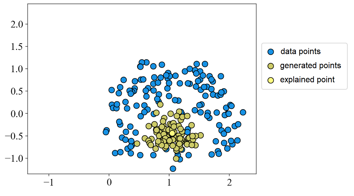
Figure 2: An example of the one-cluster data structure with the dataset points, an explained point, and points generated around the explained point

The second type of generated datasets consists of two clusters with different centers $p^{(1)}$ and $p^{(2)}$ of feature vectors and different vectors of the Cox model coefficients $\mathbf{b}_{1}^{true}$ and $\mathbf{b}_{2}^{true}$. The reason for using such a two-cluster data structure is to try to complicate the Cox model data structure. If examples are distributed according to the Cox model, then it is likely that the Cox explanation model underlying SurvLIME will provide a more accurate explanation than SurvBeX. Therefore, it is proposed to use two data clusters for a correct comparison of the models.

Parameters of the cluster generation also depend on the number of features $d$. For the numbers of features $d=5$, $d=10$, and $d=20$, they are

1. $d=5$:

   1. $\mathbf{b}_{1}^{true}=(0.5,0.25,0.12,0,0)$;

   2. $\mathbf{b}_{2}^{true}$ $=(0,0,0.12,0.25,0.5)$;

2. $d=10$:

   1. $\mathbf{b}_{1}^{true}$ $=(0.6,0.3,0.1,0,0,...,0)$;

   2. $\mathbf{b}_{2}^{true}$ $=(0,0,...,0,0.1,0.3,0.6);$

3. $d=20$:

   1. $\mathbf{b}_{1}^{true}$ $=(0.5,0.25,0.12,0,0,...,0)$;

   2. $\mathbf{b}_{2}^{true}$ $=(0,0,...,0,0.12,0.25,0.5).$

The following parameters for points of every cluster are used:

1. cluster 1: center $p^{(1)}=(0.25,0.25,0.25,0.25,0.25)$; radius $R=0.2$; the number of points in the cluster $n=200$;

2. cluster 2: center $p^{(2)}=(0.75,0.75,0.75,0.75)$; radius $R=0.2$; the number of points in the cluster $n=200$.

Parameters of the Weibull distribution for generating survival times are $\lambda=10^{-5}$, $v=2$. The total number of generated points $(\mathbf{x}_{i},\delta_{i},T_{i})$ in the dataset consisting of two clusters is $n=400$. The total number of generated points around an explained example is $N=100$. Parameters of the generation are the same as in experiments with one cluster. An example of the two-cluster data structure generated in accordance with the above parameters by using the t-SNE method is depicted in Fig.3.

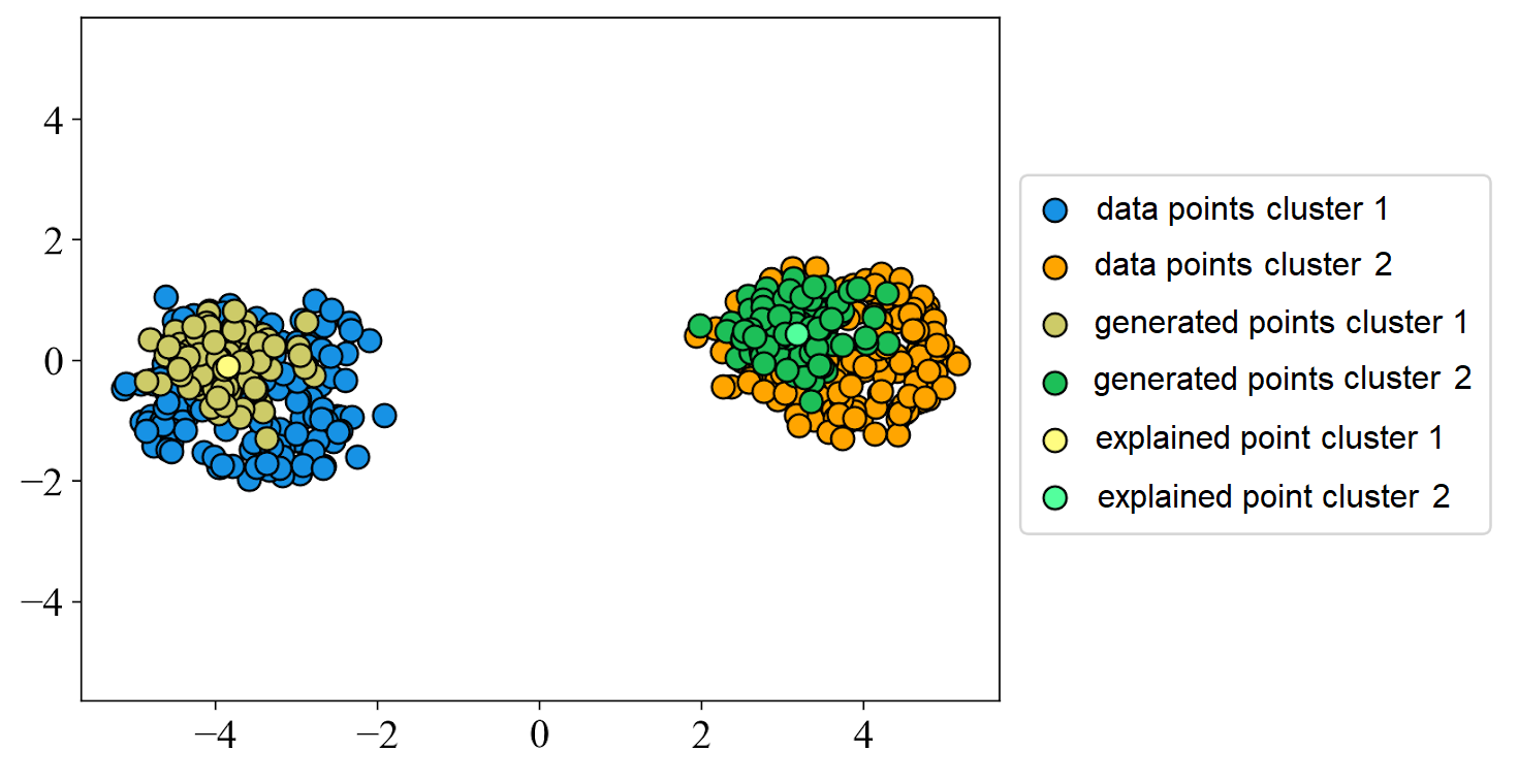
Figure 3: An example of the two-cluster data structure with the dataset points, an explained point, and points generated around the explained point in each cluster

6.2 Measures for comparison the models

To compare different models (SurvLIME and SurvBeX), we use the following three measures:

$$D(\mathbf{b}^{{model}},\mathbf{b}^{true})=\left\|\mathbf{b}^{{model}}-\mathbf{b}^{true}\right\|^{2},$$

$$KL(\mathbf{b}^{{model}},\mathbf{b}^{true})=\sum_{i=1}^{n}b_{i}^{true}\ln\frac{b_{i}^{true}}{b_{i}^{{model}}},$$

$$C(\mathbf{b}^{{model}},\mathbf{b}^{true})=\frac{\sum\nolimits_{i,j}\mathbf{1}[b_{i}^{true}<b_{j}^{true}]\cdot\mathbf{1}[b_{i}^{{model}}<b_{j}^{{model}}]}{\sum\nolimits_{i,j}\mathbf{1}[b_{i}^{true}<b_{j}^{true}]}.$$

The first measure represents the Euclidean distance between the two vectors $\mathbf{b}^{{model}}$ and $\mathbf{b}^{true}$, where the vector $\mathbf{b}^{{model}}$ is obtained by SurvLIME and SurvBeX. The vectors $\mathbf{b}^{{model}}$ and $\mathbf{b}^{true}$ are normalized. Therefore, they can be regarded as the probability distributions and the Kullback–Leibler divergence (KL) can be applied to analyze the difference between the vectors, which is used as the second measure. The third measure is the C-index applied to the vectors $\mathbf{b}^{{model}}$ and $\mathbf{b}^{true}$. It estimates the probability that any pair of vectors $\mathbf{b}^{{model}}$ and $\mathbf{b}^{true}$ are correctly ranking. It should be noted that the third index is the most informative because it estimates the relationship between elements of two vectors. The Euclidean distance and the KL-divergence show how the vectors are close to each other, but they do not show the relationship between elements of two vectors. Nevertheless, these measures can be also useful when the models are compared.

In order to study how SFs predicted by using different methods, including the black-box, SurvLIME, and SurvBeX, are close to each other, we use the following distance measure:

$$D(S,S_{B-B})=\sum_{i=1}^{n}\left(S^{(i)}(\mathbf{z})-S_{B-B}^{(i)}(\mathbf{z})\right)^{2}\left(t_{i}-t_{i-1}\right),$$ (24)

where $S^{(i)}(\mathbf{z})$ is the SF predicted by SurvLIME or SurvBeX for the explained point $\mathbf{z}$ in the time interval $[t_{i-1},t_{i}]$; $S_{B-B}^{(i)}$ is the SF predicted by the black-box model in the same time interval.

When $M$ points are used for explanation, then the mean values of the above measures are computed: mean squared distance (MSD), which can be viewed as an analog of the mean squared error (MSE), mean KL-divergence (MKL), mean C-index (MCI), and mean SF distance (MSFD). The above measures are computed similarly, for example, the MSD is determined as

$$MSD=\frac{1}{M}\sum_{i=1}^{M}D(\mathbf{b}_{i}^{{model}},\mathbf{b}^{true}),$$

where $\mathbf{b}_{i}^{{model}}$ is the vector obtained by solving (18) for the $i$-th explained point by using SurvLIME or SurvBeX.

The greater the value of the MCI and the smaller the MSFD, the MKL, and the MSD, the better results we get.

6.3 One cluster

First, we compare SurvBeX with SurvLIME by generating one cluster as it is shown in Fig.2. The first black-box model is the Cox model which is used in order to be sure that SurvLIME provides correct results. It is important to point out the following observation. If the Cox model uses the same method for computing the baseline SF $S_{0}(t\mathbf{)}$ (see the corresponding expression (5)), then SurvLIME provides outperforming results because it actually tries to minimize the distance between SFs which are similar to some extent. In this case, we obtain outperforming results provided by SurvLIME. The outperformance is also supported by the fact that the training set is generated in accordance with probability distributions satisfying the Cox model.

Boxplots in Fig.4 show differences between MSFD, MSD, MKL, and MCI for SurvLIME and SurvBeX when the black box is the Cox model. It can be seen from Fig.4 that SurvLIME provides better results in comparison with SurvBeX in accordance with all introduced measures. The results justify the above assumption about comparison of SurvLIME and SurvBeX when the black box is the Cox model and training example are generated in accordance with the Cox model.

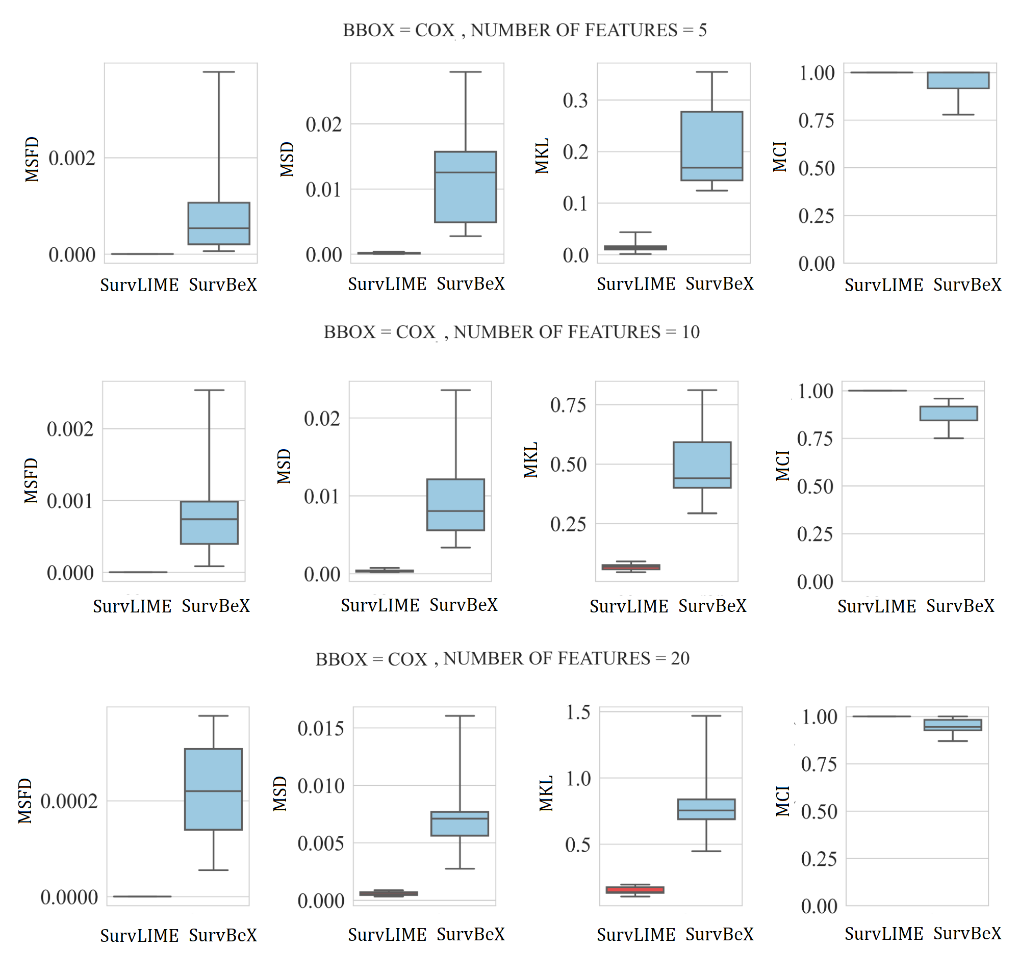
Figure 4: Boxplots illustrating difference between MSFD, MSD, MKL, and MCI for SurvLIME and SurvBeX when the black box is the Cox model and numbers of features are 5, 10, 20

Fig.5 shows values of the feature importance (the left column) and SFs provided by the black box, SurvLIME and SurvBeX (the right column) under the same conditions. For each number of features in examples of the generated dataset, an explained example is randomly selected from the dataset. Results of the explanation and the corresponding SFs provided by different models are depicted. It can be seen from Fig.5 that SFs produced by the black-box model (depicted by the thicker line) and SurvLIME almost coincide whereas SF produced by SurvBeX differs from the black-box model SF. At the same time, when the number of features is 20, SurvBeX provides results similar to SurvLIME.

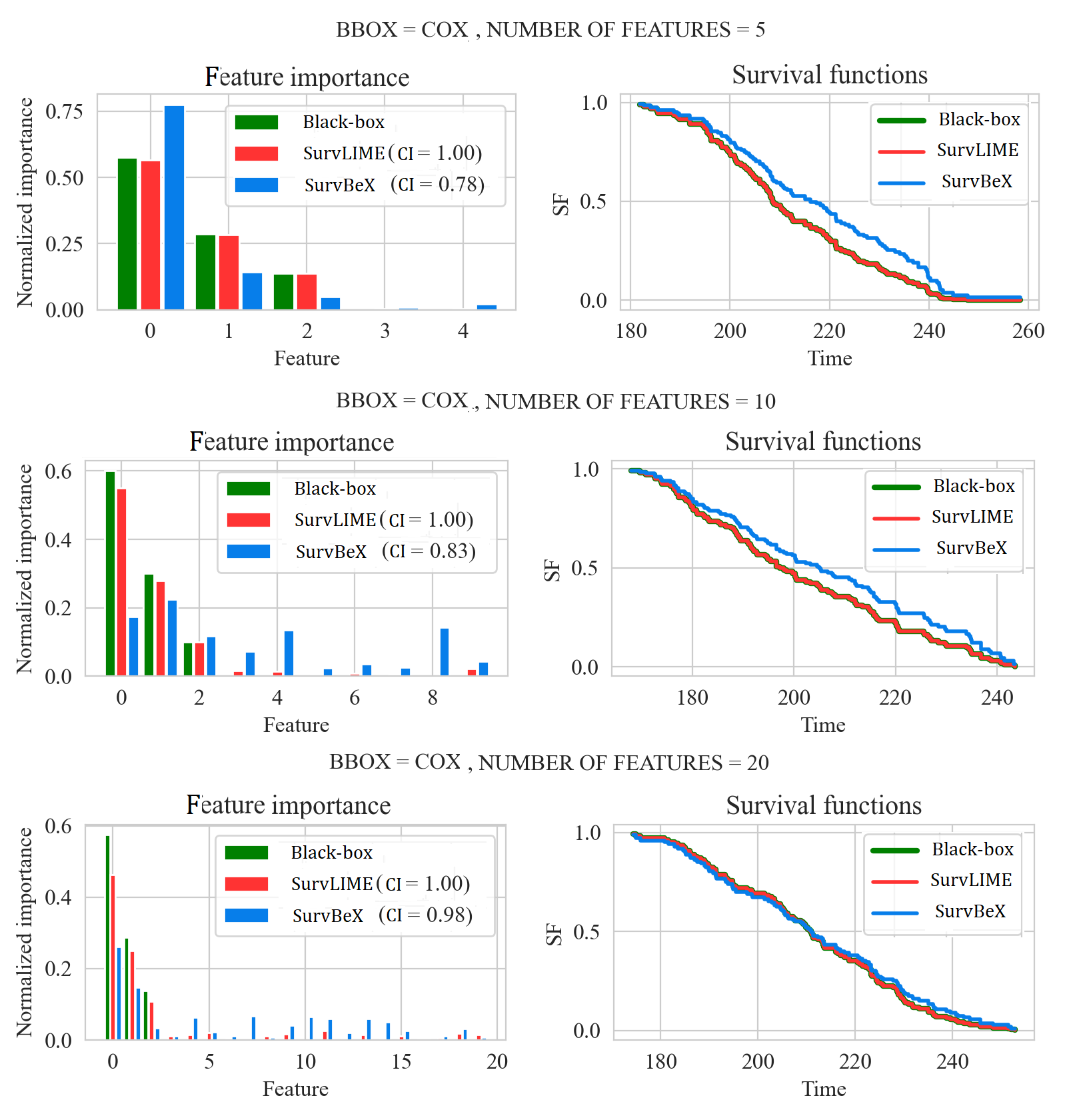
Figure 5: Values of the feature importance (the left column) and SFs provided by the black-box model (the Cox model), SurvLIME, and SurvBeX (the right column)

Let us consider the RSF as a black-box model. The corresponding numerical results are shown in Figs.6-7.

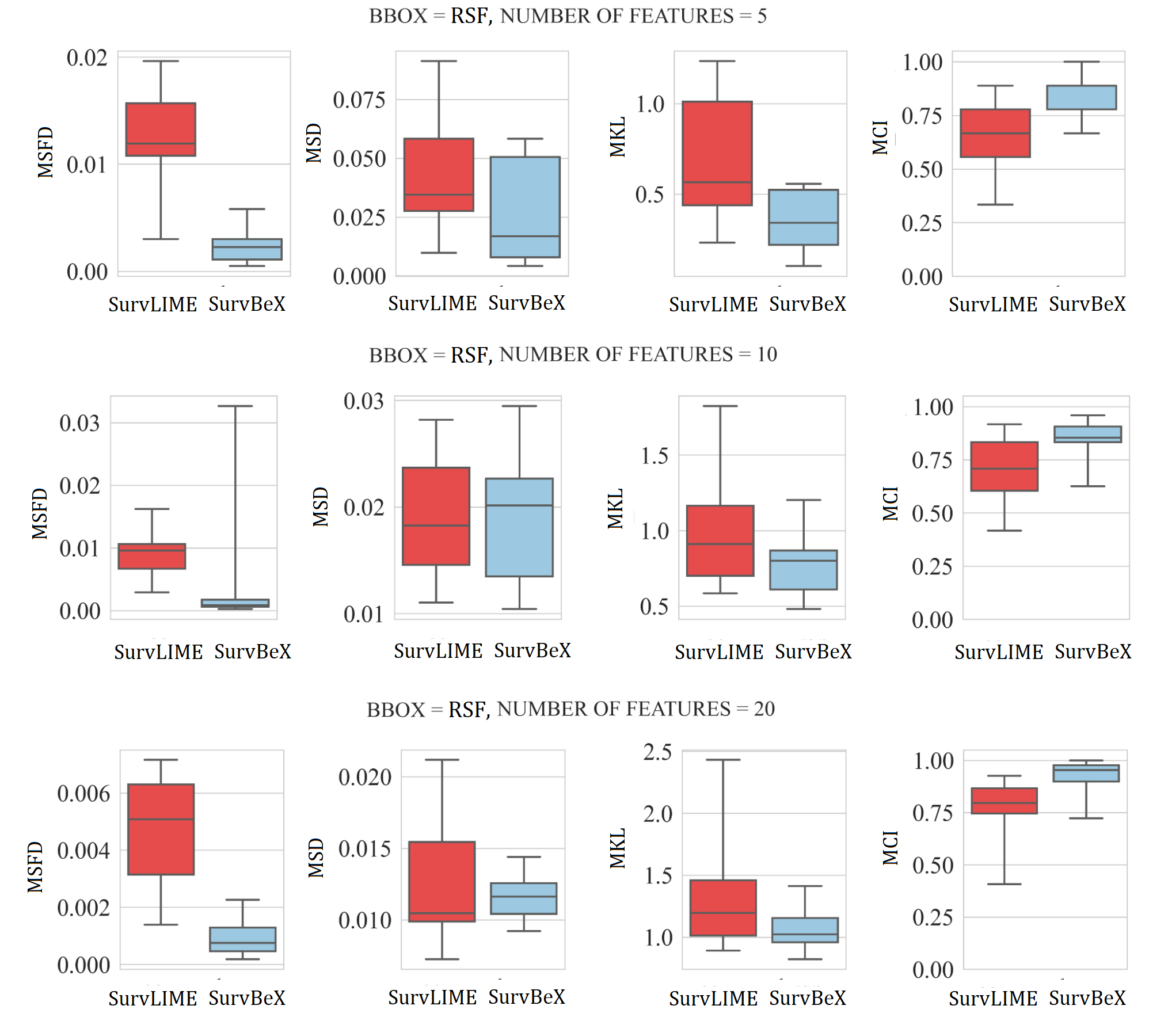
Figure 6: Boxplots illustrating difference between MSFD, MSD, MKL, and MCI for SurvLIME and SurvBeX when the black box is the RSF and numbers of features are 5, 10, 20

Fig.6 shows boxplots of MSFD, MSD, MKL, and MCI for SurvLIME and SurvBeX when the black box is the RSF. It is interesting to note that SurvBeX provides better results in comparison with SurvLIME. It is interesting also to point out that SurvBeX behaves more stable when the number of features increases. It can be also seen from Fig.6 (boxplots of MSFD) that the SurvBeX provides better approximation of the SF because the MSFD measures for SurvBeX are smaller than the same measures for SurvLIME. The same conclusion is supported by Fig.7 where randomly selected explained examples for three cases of the feature numbers are analyzed. It can be seen from Fig.7 that SFs provided by SurvBeX are much closer to the black-box SF in comparison with SFs produced by SurvLIME. The difference between results obtained by different black-box models can be explained by the fact that, in spite of the training set generated by using the Cox model, the RSF produces the SF different from the “ideal” SF corresponding to the Cox model and this difference increases with the number of features. The Beran estimator is more sensitive to the changes of SFs and, therefore, SurvBeX provides better results.

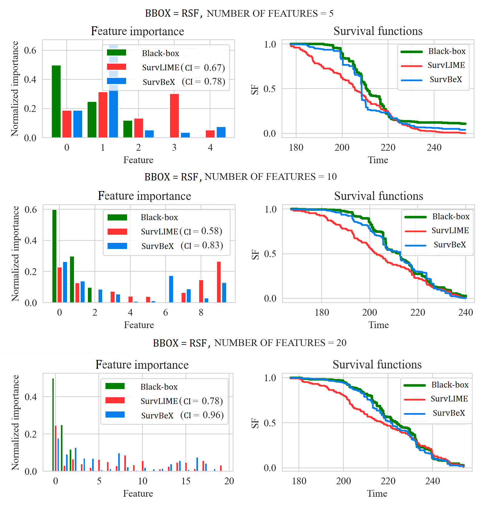
Figure 7: Values of the feature importance (the left column) and SFs provided by the black-box model (the RSF), SurvLIME, and SurvBeX (the right column)

In order to study different cases of the black-box models, we use the Beran estimator as a black-box model. It is obvious in this case that SurvBeX should provide outperforming results. This assumption is justified by results shown in Fig.8. One can see from Fig.8 that SurvBeX outperforms SurvLIME for all numbers of features. The same can be seen from Fig.9. SFs produced by SurvBeX are closer to the black-box SFs than SFs produced by SurvLIME.

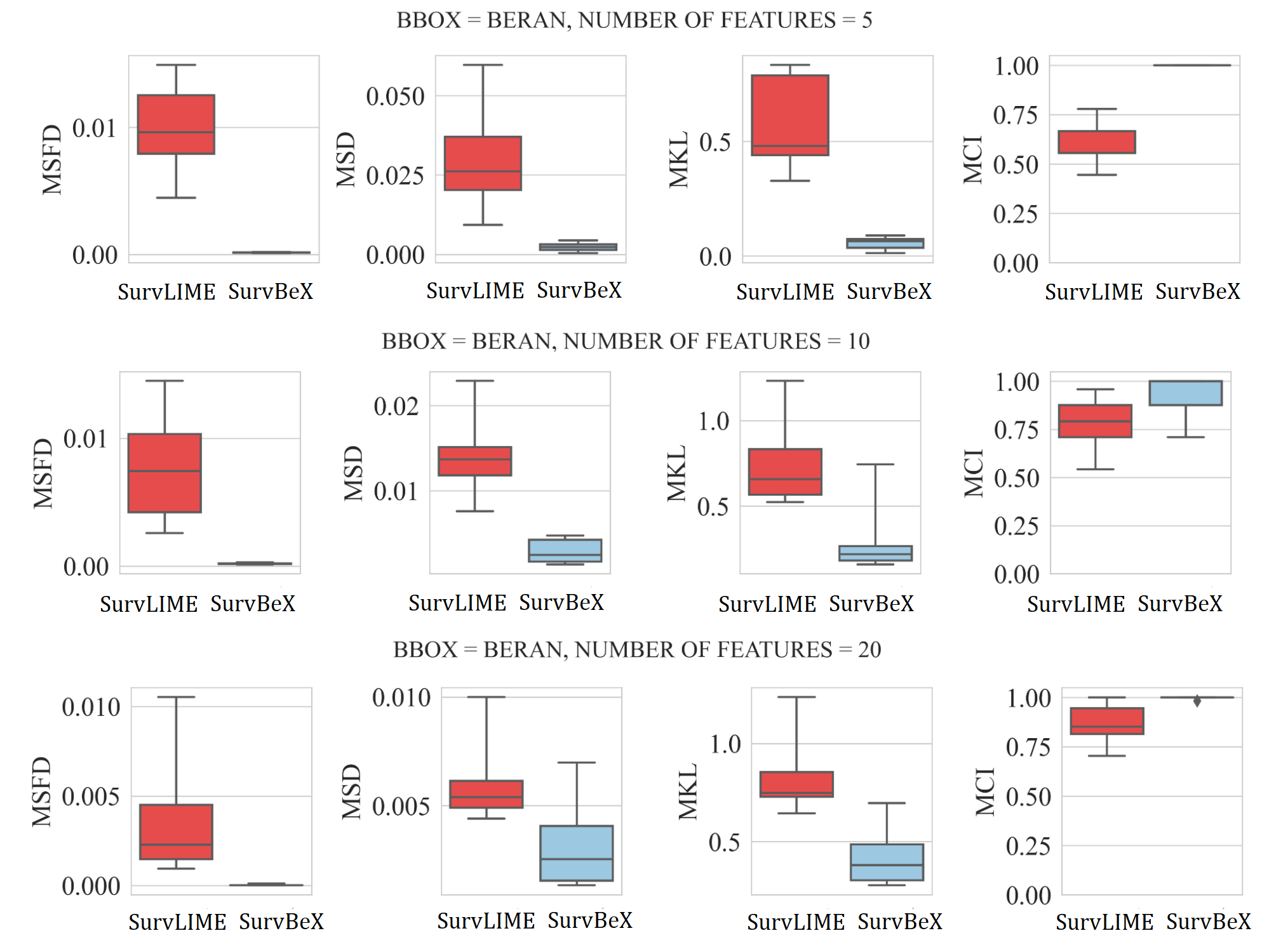
Figure 8: Boxplots illustrating difference between MSFD, MSD, MKL, and MCI for SurvLIME and SurvBeX when the black box is the Beran estimator

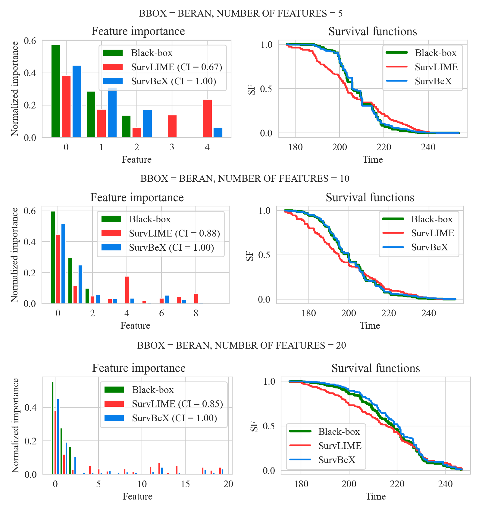
Figure 9: Values of the feature importance (the left column) and SFs provided by the Beran estimator as a black-box model, SurvLIME, and SurvBeX (the right column)

6.4 Two clusters

Let us compare SurvBeX with SurvLIME when two clusters of examples are generated (see Fig.3) such that the clusters are generated in accordance with the Cox model, but they have quite different parameters of the model. It is obvious that this data structure entirely violates the homogeneous Cox model data structure. Therefore, it can be assumed in advance that SurvLIME will produce worse results. This is confirmed by the following experiments.

We consider the case when the RSF is used as a black box. Fig.10 shows boxplots of MSFD, MSD, MKL, and MCI for SurvLIME and SurvBeX. It can be seen from Fig.10 that SurvBeX provides better results for different numbers of features. At the same time, the outperformance of SurvBeX is reduced with increase of the feature numbers.

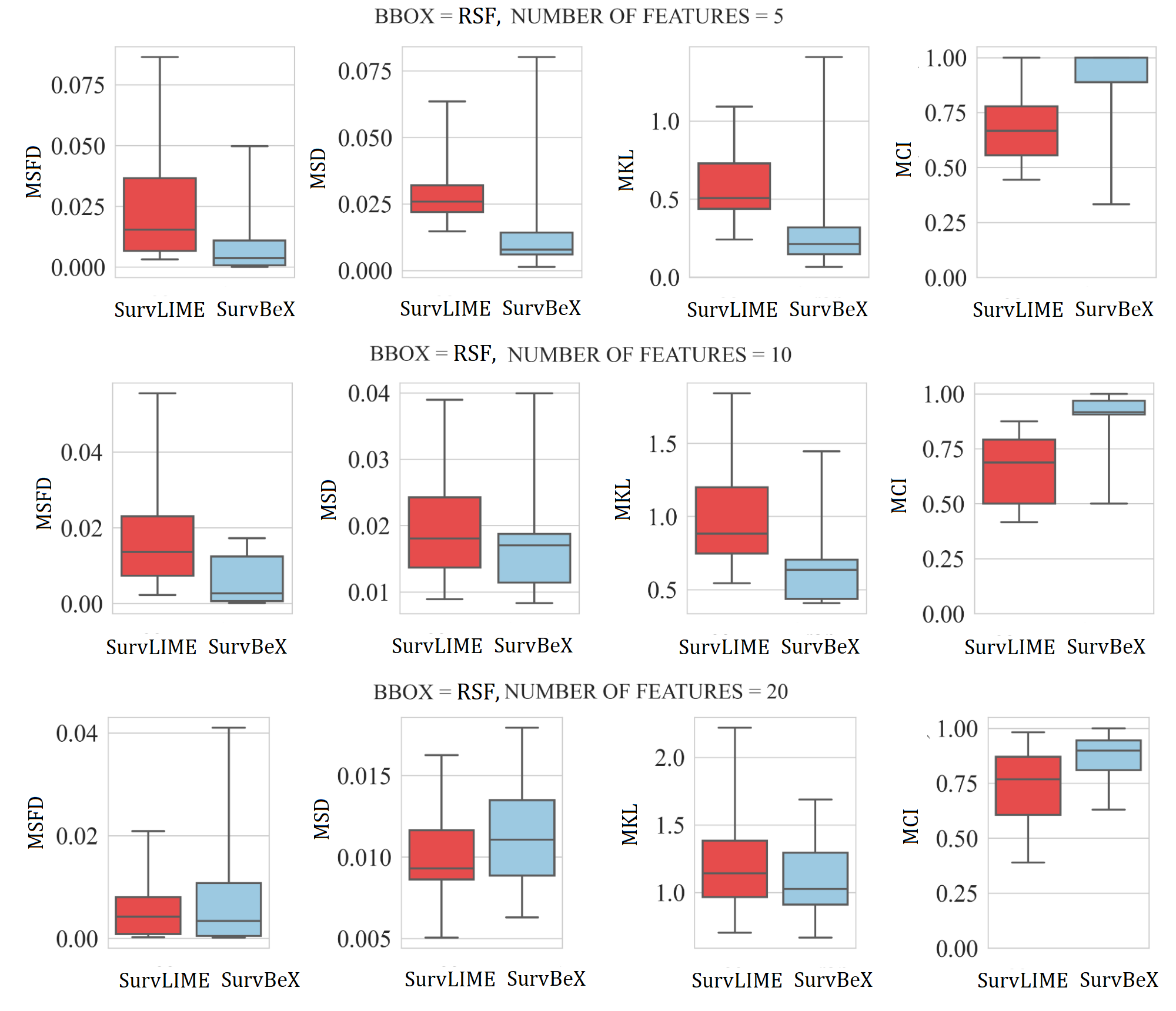
Figure 10: Boxplots illustrating difference between MSFD, MSD, MKL, and MCI for SurvLIME and SurvBeX when the black box is the RSF and two clusters of training data are used

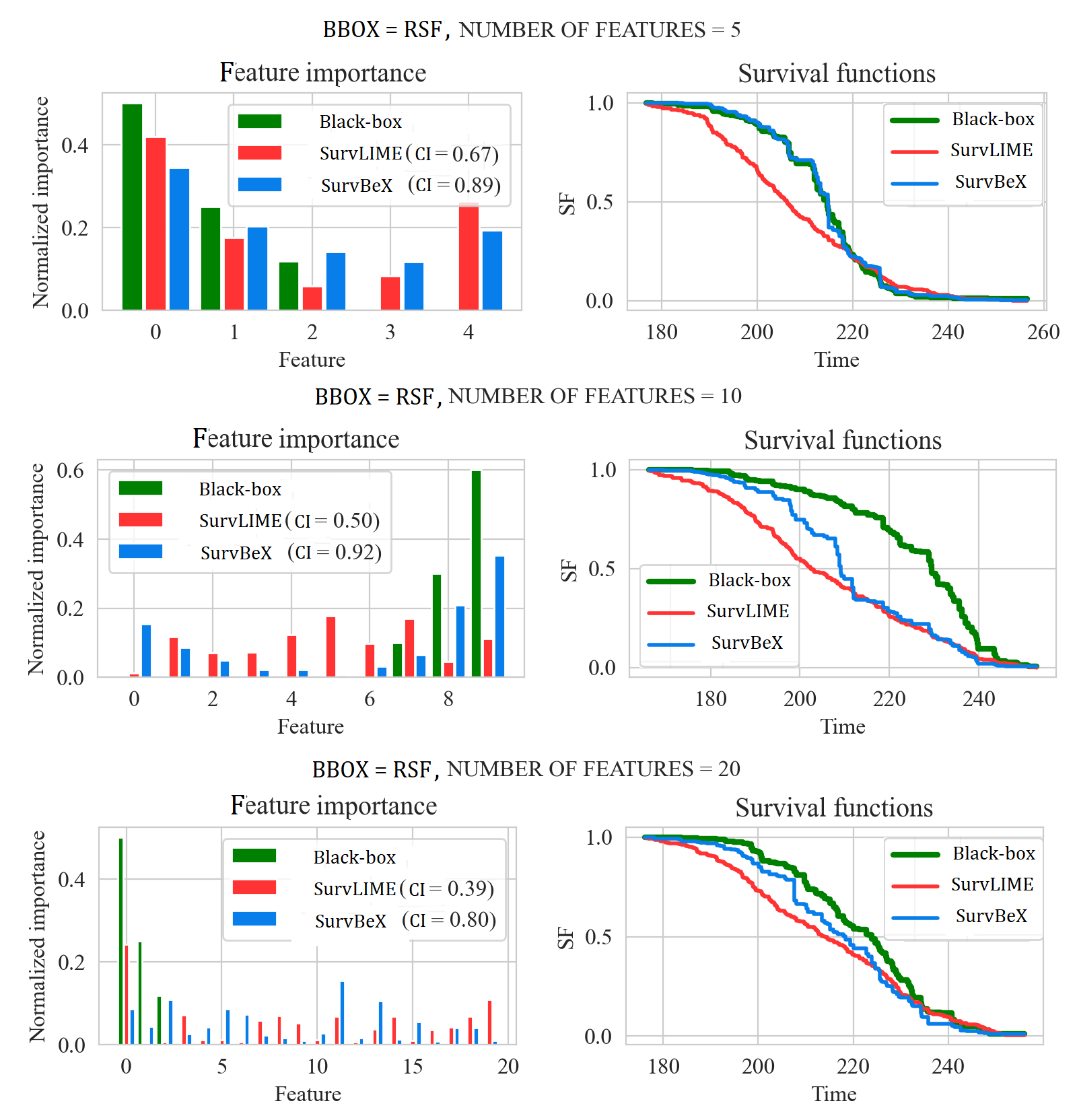
Figure 11: Values of the feature importance (the left column) and SFs provided by the RSF as a black-box model, SurvLIME, and SurvBeX (the right column) when two clusters are used

An important peculiarity of the RSF as a black-box model is that it tries to separate examples from different clusters. As a result, the produced SF for each point strongly depends on a cluster which contains the point. In contrast to the RSF, the Cox model computes the baseline SF $S_{0}(t)$ which is common for all points of clusters. Therefore, the Cox model as a black-box model “averages” the clusters and provides the unsatisfactory prediction results. In particular, C-indices of the Cox black-box model computed on the training and testing sets of the two-cluster dataset with five features are $0.59$ and $0.57$, respectively, whereas C-indices of the black-box RSF are $0.95$ and $0.91$, respectively. We can see that the Cox black-box model is no better than random guessing. Fig.12 shows boxplots of MSFD, MSD, MKL, and MCI for this case. It seems from Fig.12 that SurvBeX is worse than SurvLIME. However, this is not the case. The average distance (MSFD) between SFs is very small, and explanation models simply try to guess the feature importance which is also close to $0.5$. Due to the more complex optimization in SurvBeX, the error of its explanation is greater.

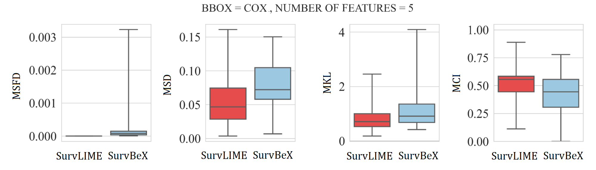
Figure 12: Boxplots illustrating difference between MSFD, MSD, MKL, and MCI for SurvLIME and SurvBeX when the black box is the Cox model and the training dataset consists of two clusters

Table 1 illustrate the relationship between different explanation methods when two clusters are considered, the black-box is the RSF, and the number of features in training examples is 5. We also consider an additional explanation method called SurvSHAP [29]. Mean values and standard deviations of measures MSD, MKL, and MCI are given in Table 1. It can be seen from the table that SurvBeX outperforms other explanation methods. Similar results by $10$ features are shown in Table 2.

Table 1: Mean values and standard deviations of measures MSD, MKL, and MCI for SurvBex, SurvLIME, and SurvSHAP by 5 features

Method	MSD	MKL	MCI
SurvBeX	$0.004\pm 0.002$	$0.129\pm 0.052$	$0.956\pm 0.057$
SurvLIME	$0.032\pm 0.017$	$0.621\pm 0.343$	$0.685\pm 0.176$
SurvSHAP	$0.044\pm 0.005$	$0.629\pm 0.069$	$0.581\pm 0.214$

Table 2: Mean values and standard deviations of measures MSD, MKL, and MCI for SurvBex, SurvLIME, and SurvSHAP by 10 features

Method	MSD	MKL	MCI
SurvBeX	$0.016\pm 0.004$	$0.665\pm 0.151$	$0.825\pm 0.140$
SurvLIME	$0.016\pm 0.005$	$0.862\pm 0.215$	$0.642\pm 0.139$
SurvSHAP	$0.035\pm 0.002$	$1.347\pm 0.107$	$0.583\pm 0.192$

7 Numerical experiments with real data

To illustrate SurvBeX, we study it on the following well-known real datasets:

• The Veterans’ Administration Lung Cancer Study (Veteran) Dataset [81] contains data on 137 males with advanced inoperable lung cancer. The subjects were randomly assigned to either a standard chemotherapy treatment or a test chemotherapy treatment. Several additional variables were also measured on the subjects. The dataset can be obtained via the “survival” R package or the Python “scikit-survival” package..

• The German Breast Cancer Study Group 2 (GBSG2) Dataset contains observations of 686 women [82]. Every example is characterized by 10 features, including age of the patients in years, menopausal status, tumor size, tumor grade, number of positive nodes, hormonal therapy, progesterone receptor, estrogen receptor, recurrence free survival time, censoring indicator (0 - censored, 1 - event). The dataset can be obtained via the “TH.data” R package or the Python “scikit-survival” package.

• The Worcester Heart Attack Study (WHAS500) Dataset [1] describes factors associated with acute myocardial infarction. It considers 500 patients with 14 features. The endpoint is death, which occurred for 215 patients (43.0%). The dataset can be obtained via the “smoothHR” R package or the Python “scikit-survival” package.‘

Fig.13(a) shows the data structure of the dataset Veteran by means of the t-SNE method. Fig.13(b) shows SFs predicted by the black-box model, SurvLIME and SurvBeX. It can be seen from Fig.13 that the dataset has a specific structure which does not allows us to construct a proper Cox model in the framework of SurvLIME. As a result, the SF produced by SurvBeX is closer to the SF predicted by the black-box model than the SF produced by SurvLIME. Mean values of the feature importance over all points of the dataset computed by using SurvLIME and SurvBeX are depicted in Fig.13(c). It can be seen from Fig.13(c) that the results provided by SurvLIME and SurvBeX are different. The methods coincide in selection of the most important feature “Karnofsky score”. However, the most important second feature is determined by SurvBeX as “Celltype” whereas SurvLIME determines it as “Months from diagnosis”. “Karnofsky score” and “Celltype” as the most important features were determined also in [70].

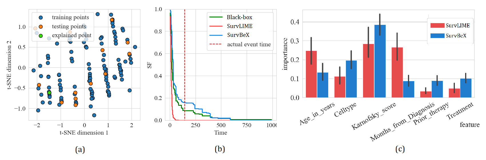
Figure 13: Experiments with the Veteran dataset: (a) the t-SNE representation of data; (b) SFs predicted by the black-box model, SurvLIME and SurvBeX; (c) mean values of the feature importance

The next dataset for studying is GBSG2. The data structure of the dataset GBSG2 depicted by means of the t-SNE method and SFs predicted by the black-box model SurvLIME and SurvBeX are shown in Fig.14(a) and (b), respectively, We again see that the SF produced by SurvBeX is closer to the SF predicted by the black-box model than the SF produced by SurvLIME. Fig.14(c) shows mean values of the feature importance over all points of the dataset GBSG2 computed by using SurvLIME and SurvBeX.

The same results can be seen in Fig.15 where results obtained for the dataset WHAS500 are shown.

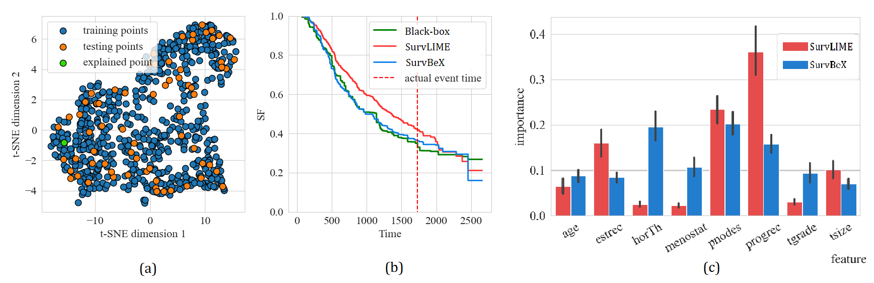
Figure 14: Experiments with the GBSG2 dataset: (a) the t-SNE representation of data; (b) SFs predicted by the black-box model, SurvLIME and SurvBeX; (c) mean values of the feature importance

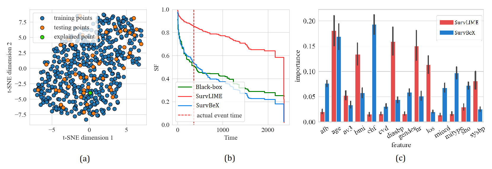
Figure 15: Experiments with the WHAS500 dataset: (a) the t-SNE representation of data; (b) SFs predicted by the black-box model, SurvLIME and SurvBeX; (c) mean values of the feature importance

8 Conclusion

A new explanation method called SurvBeX, which can be regarded as an alternative to the well-known method SurvLIME developed for survival data, has been presented in the paper. The main idea behind the method is to use the Beran estimator to approximate a survival black-box model at an explained point. The explanation by means of SurvBeX is reduced to minimization between SFs predicted by the black-box model and the Beran estimator for points generated around the explained point.

There is an important difference between SurvLIME and SurvBeX except for the use of the Beran estimator instead of the Cox model. According to SurvLIME, the importance weights $\mathbf{b}$ are assigned to features. In SurvBeX, they are assigned to distances between features of the explained example and training examples. This implies that the importance weights in SurvBeX directly depend on the training set whereas the weights in SurvLIME implicitly depend on the training set through the baseline function which may be incorrect when the analyzed dataset has a complex structure.

At the same time, we should point out a drawback of SurvBeX. In contrast to SurvLIME, SurvBeX has to solve the complex optimization problem, which leads to increasing the computation time. Nevertheless, various numerical experiments have demonstrated that the optimization problem is successfully solved and SurvBeX provides the outperforming explanation.

There are several ways for further research based on the proposed method. First of all, we have considered the minimization of the distances between SFs. In the same way, the cumulative hazard functions can be considered as it has been implemented in SurvLIME. Second, only the Gaussian kernel and its modification have been used to implement SurvBeX. However, it is interesting to consider other types of kernels which may provide outperforming results. Third, another important generalization of the proposed method is to combine SurvLIME and SurvBeX. For example, they can be linearly combined with some parameter such that the SF of the combined explanation model is represented as a linear combination of two SFs with the same parameters $\mathbf{b}$. The above problems are directions for further research.

References

- [1] D. Hosmer, S. Lemeshow, and S. May. Applied Survival Analysis: Regression Modeling of Time to Event Data. John Wiley & Sons, New Jersey, 2008.
- [2] P. Wang, Y. Li, and C.K. Reddy. Machine learning for survival analysis: A survey. ACM Computing Surveys (CSUR), 51(6):1–36, 2019.
- [3] M.Z. Nezhad, N. Sadati, K. Yang, and D. Zhu. A deep active survival analysis approach for precision treatment recommendations: Application of prostate cancer. arXiv:1804.03280v1, April 2018.
- [4] D.R. Cox. Regression models and life-tables. Journal of the Royal Statistical Society, Series B (Methodological), 34(2):187–220, 1972.
- [5] C. Haarburger, P. Weitz, O. Rippel, and D. Merhof. Image-based survival analysis for lung cancer patients using CNNs. arXiv:1808.09679v1, Aug 2018.
- [6] J.L. Katzman, U. Shaham, A. Cloninger, J. Bates, T. Jiang, and Y. Kluger. Deepsurv: Personalized treatment recommender system using a Cox proportional hazards deep neural network. BMC medical research methodology, 18(24):1–12, 2018.
- [7] D.M. Witten and R. Tibshirani. Survival analysis with high-dimensional covariates. Statistical Methods in Medical Research, 19(1):29–51, 2010.
- [8] X. Zhu, J. Yao, and J. Huang. Deep convolutional neural network for survival analysis with pathological images. In 2016 IEEE International Conference on Bioinformatics and Biomedicine, pages 544–547. IEEE, 2016.
- [9] F.M. Khan and V.B. Zubek. Support vector regression for censored data (SVRc): a novel tool for survival analysis. In 2008 Eighth IEEE International Conference on Data Mining, pages 863–868. IEEE, 2008.
- [10] N.A. Ibrahim, A. Kudus, I. Daud, and M.R. Abu Bakar. Decision tree for competing risks survival probability in breast cancer study. International Journal Of Biological and Medical Research, 3(1):25–29, 2008.
- [11] U.B. Mogensen, H. Ishwaran, and T.A. Gerds. Evaluating random forests for survival analysis using prediction error curves. Journal of Statistical Software, 50(11):1–23, 2012.
- [12] M. Schmid, M.N. Wright, and A. Ziegler. On the use of harrell’s c for clinical risk prediction via random survival forests. Expert Systems with Applications, 63:450–459, 2016.
- [13] H. Wang and L. Zhou. Random survival forest with space extensions for censored data. Artificial intelligence in medicine, 79:52–61, 2017.
- [14] M.N. Wright, T. Dankowski, and A. Ziegler. Unbiased split variable selection for random survival forests using maximally selected rank statistics. Statistics in Medicine, 36(8):1272–1284, 2017.
- [15] S. Wiegrebe, P. Kopper, R. Sonabend, and A. Bender. Deep learning for survival analysis: A review. arXiv:2305.14961, May 2023.
- [16] A. Holzinger, G. Langs, H. Denk, K. Zatloukal, and H. Muller. Causability and explainability of artificial intelligence in medicine. WIREs Data Mining and Knowledge Discovery, 9(4):e1312, 2019.
- [17] V. Arya, R.K.E. Bellamy, P.-Y. Chen, A. Dhurandhar, M. Hind, S.C. Hoffman, S. Houde, Q.V. Liao, R. Luss, A. Mojsilovic, S. Mourad, P. Pedemonte, R. Raghavendra, J. Richards, P. Sattigeri, K. Shanmugam, M. Singh, K.R. Varshney, D. Wei, and Y. Zhang. One explanation does not fit all: A toolkit and taxonomy of AI explainability techniques. arXiv:1909.03012, Sep 2019.
- [18] R. Guidotti, A. Monreale, S. Ruggieri, F. Turini, F. Giannotti, and D. Pedreschi. A survey of methods for explaining black box models. ACM computing surveys, 51(5):93, 2019.
- [19] C. Molnar. Interpretable Machine Learning: A Guide for Making Black Box Models Explainable. Published online, https://christophm.github.io/interpretable-ml-book/, 2019.
- [20] W.J. Murdoch, C. Singh, K. Kumbier, R. Abbasi-Asl, and B. Yu. Definitions, methods, and applications in interpretable machine learning. In Proceedings of the National Academy of Sciences, volume 116, pages 22071–22080, 2019.
- [21] M.T. Ribeiro, S. Singh, and C. Guestrin. “Why should I trust You?” Explaining the predictions of any classifier. arXiv:1602.04938v3, Aug 2016.
- [22] D. Garreau and U. Luxburg. Explaining the explainer: A first theoretical analysis of lime. In International Conference on Artificial Intelligence and Statistics, pages 1287–1296. PMLR, 2020.
- [23] M.S. Kovalev, L.V. Utkin, and E.M. Kasimov. SurvLIME: A method for explaining machine learning survival models. Knowledge-Based Systems, 203:106164, 2020.
- [24] M.S. Kovalev and L.V. Utkin. A robust algorithm for explaining unreliable machine learning survival models using the Kolmogorov-Smirnov bounds. Neural Networks, 132:1–18, 2020.
- [25] L.V. Utkin, M.S. Kovalev, and E.M. Kasimov. An explanation method for black-box machine learning survival models using the chebyshev distance. In Artificial Intelligence and Natural Language. AINL 2020, volume 1292 of Communications in Computer and Information Science, pages 62–74, Cham, 2020. Springer.
- [26] R. Beran. Nonparametric regression with randomly censored survival data. Technical report, University of California, Berkeley, 1981.
- [27] S.M. Lundberg and S.-I. Lee. A unified approach to interpreting model predictions. In Advances in Neural Information Processing Systems, pages 4765–4774, 2017.
- [28] E. Strumbelj and I. Kononenko. An efficient explanation of individual classifications using game theory. Journal of Machine Learning Research, 11:1–18, 2010.
- [29] M. Krzyzinski, M. Spytek, H. Baniecki, and P. Biecek. SurvSHAP (t): Time-dependent explanations of machine learning survival models. Knowledge-Based Systems, 262:110234, 2023.
- [30] S.M. Shankaranarayana and D. Runje. ALIME: Autoencoder based approach for local interpretability. arXiv:1909.02437, Sep 2019.
- [31] I. Ahern, A. Noack, L. Guzman-Nateras, D. Dou, B. Li, and J. Huan. NormLime: A new feature importance metric for explaining deep neural networks. arXiv:1909.04200, Sep 2019.
- [32] M.R. Zafar and N.M. Khan. DLIME: A deterministic local interpretable model-agnostic explanations approach for computer-aided diagnosis systems. arXiv:1906.10263, Jun 2019.
- [33] M.T. Ribeiro, S. Singh, and C. Guestrin. Anchors: High-precision model-agnostic explanations. In AAAI Conference on Artificial Intelligence, pages 1527–1535, 2018.
- [34] L. Hu, J. Chen, V.N. Nair, and A. Sudjianto. Locally interpretable models and effects based on supervised partitioning (LIME-SUP). arXiv:1806.00663, Jun 2018.
- [35] J. Rabold, H. Deininger, M. Siebers, and U. Schmid. Enriching visual with verbal explanations for relational concepts: Combining LIME with Aleph. arXiv:1910.01837v1, October 2019.
- [36] Q. Huang, M. Yamada, Y. Tian, D. Singh, D. Yin, and Y. Chang. GraphLIME: Local interpretable model explanations for graph neural networks. arXiv:2001.06216, January 2020.
- [37] T. Chowdhury, R. Rahimi, and J. Allan. Rank-lime: Local model-agnostic feature attribution for learning to rank. arXiv:2212.12722, Dec 2022.
- [38] R. Gaudel, L. Galarraga, J. Delaunay, L. Roze, and V. Bhargava. s-lime: Reconciling locality and fidelity in linear explanations. arXiv:2208.01510, Aug 2022.
- [39] Heewoo Jun and A. Nichol. Shap-e: Generating conditional 3d implicit functions. arXiv:2305.02463, May 2023.
- [40] F. Fumagalli, M. Muschalik, P. Kolpaczki, E. Hullermeier, and B. Hammer. Shap-iq: Unified approximation of any-order shapley interactions. arXiv:2303.01179, Mar 2023.
- [41] A. Coletta, S. Vyetrenko, and T. Balch. K-shap: Policy clustering algorithm for anonymous multi-agent state-action pairs. arXiv:2302.11996, Feb 2023.
- [42] L. Parcalabescu and A. Frank. Mm-shap: A performance-agnostic metric for measuring multimodal contributions in vision and language models and tasks. arXiv:2212.08158, Dec 2022.
- [43] R. Bitto, A. Malach, A. Meiseles, S. Momiyama, T. Araki, J. Furukawa, Y. Elovici, and A. Shabtai. Latent shap: Toward practical human-interpretable explanations. arXiv:2211.14797, Nov 2022.
- [44] L. Bouneder, Y. Leo, and A. Lachapelle. X-SHAP: towards multiplicative explainability of machine learning. arXiv:2006.04574, June 2020.
- [45] L.V. Utkin and A.V. Konstantinov. Ensembles of random shaps. Algorithms, 15(11):431, 2022.
- [46] T. Hastie and R. Tibshirani. Generalized additive models, volume 43. CRC press, 1990.
- [47] H. Nori, S. Jenkins, P. Koch, and R. Caruana. InterpretML: A unified framework for machine learning interpretability. arXiv:1909.09223, September 2019.
- [48] C.-H. Chang, S. Tan, B. Lengerich, A. Goldenberg, and R. Caruana. How interpretable and trustworthy are gams? arXiv:2006.06466, June 2020.
- [49] R. Agarwal, N. Frosst, X. Zhang, R. Caruana, and G.E. Hinton. Neural additive models: Interpretable machine learning with neural nets. arXiv:2004.13912, April 2020.
- [50] Z. Yang, A. Zhang, and A. Sudjianto. Gami-net: An explainable neural networkbased on generalized additive models with structured interactions. arXiv:2003.07132, March 2020.
- [51] J. Chen, J. Vaughan, V.N. Nair, and A. Sudjianto. Adaptive explainable neural networks (AxNNs). arXiv:2004.02353v2, April 2020.
- [52] A. Adadi and M. Berrada. Peeking inside the black-box: A survey on explainable artificial intelligence (XAI). IEEE Access, 6:52138–52160, 2018.
- [53] A.B. Arrieta, N. Diaz-Rodriguez, J. Del Ser, A. Bennetot, S. Tabik, A. Barbado, S. Garcia, S. Gil-Lopez, D. Molina, R. Benjamins, R. Chatila, and F. Herrera. Explainable artificial intelligence (XAI): Concepts, taxonomies, opportunities and challenges toward responsible AI. Information Fusion, 58:82–115, 2020.
- [54] F. Bodria, F. Giannotti, R. Guidotti, F. Naretto, D. Pedreschi, and S. Rinzivillo. Benchmarking and survey of explanation methods for black box models. Data Mining and Knowledge Discovery, 2023.
- [55] N. Burkart and M.F. Huber. A survey on the explainability of supervised machine learning. Journal of Artificial Intelligence Research, 70:245–317, 2021.
- [56] D.V. Carvalho, E.M. Pereira, and J.S. Cardoso. Machine learning interpretability: A survey on methods and metrics. Electronics, 8(832):1–34, 2019.
- [57] A. Cwiling, V. Perduca, and O. Bouaziz. A comprehensive framework for evaluating time to event predictions using the restricted mean survival time. arXiv:2306.16075, Jun 2023.
- [58] C. Rudin. Stop explaining black box machine learning models for high stakes decisions and use interpretable models instead. Nature Machine Intelligence, 1:206–215, 2019.
- [59] S. Bobrowski, Hong Chen, M. Doring, U. Jensen, and W. Schinkothe. Estimation of the lifetime distribution of mechatronic systems in the presence of a covariate: A comparison among parametric, semiparametric and nonparametric models. Reliability Engineering & System Safety, 139:105–112, 2015.
- [60] K.E. Gneyou. A strong linear representation for the maximum conditional hazard rate estimator in survival analysis. Journal of Multivariate Analysis, 128:10–18, 2014.
- [61] R. Pelaez, R. Cao, and J.M. Vilar. Nonparametric estimation of the conditional survival function with double smoothing. Journal of Nonparametric Statistics, 2022. Published online.
- [62] I. Selingerova, S. Katina, and I. Horova. Comparison of parametric and semiparametric survival regression models with kernel estimation. Journal of Statistical Computation and Simulation, 91(13):2717–2739, 2021.
- [63] G. Tutz and L. Pritscher. Nonparametric estimation of discrete hazard functions. Lifetime Data Analysis, 2(3):291–308, 1996.
- [64] R. Pelaez, R. Cao, and J.M. Vilar. Probability of default estimation in credit risk using a nonparametric approach. TEST, 30:383–405, 2021.
- [65] A. Widodo and B.-S. Yang. Machine health prognostics using survival probability and support vector machine. Expert Systems with Applications, 38(7):8430–8437, 2011.
- [66] D. Faraggi and R. Simon. A neural network model for survival data. Statistics in medicine, 14(1):73–82, 1995.
- [67] S. Kaneko, A. Hirakawa, and C. Hamada. Enhancing the lasso approach for developing a survival prediction model based on gene expression data. Computational and Mathematical Methods in Medicine, 2015(Article ID 259474):1–7, 2015.
- [68] N. Ternes, F. Rotolo, and S. Michiels. Empirical extensions of the lasso penalty to reduce the false discovery rate in high-dimensional cox regression models. Statistics in medicine, 35(15):2561–2573, 2016.
- [69] C. Pachon-Garcia, C. Hernandez-Perez, P. Delicado, and V. Vilaplana. SurvLIMEpy: A python package implementing SurvLIME. arXiv:2302.10571, Feb 2023.
- [70] L.V. Utkin, E.D. Satyukov, and A.V. Konstantinov. SurvNAM: The machine learning survival model explanation. Neural Networks, 147:81–102, 2022.
- [71] M. Peroni, M. Kurban, Sun Young Yang, Young Sun Kim, Hae Yeon Kang, and Ji Hyun Song. Extending the neural additive model for survival analysis with ehr data. arXiv:2211.07814, Nov 2022.
- [72] Xinxing Wu, Chong Peng, R. Charnigo, and Qiang Cheng. Explainable censored learning: Finding critical features with long term prognostic values for survival prediction. arXiv:2209.15450, Sep 2022.
- [73] A. Moncada-Torres, M.C. van Maaren, M.P. Hendriks, S. Siesling, and G. Geleijnse. Explainable machine learning can outperform cox regression predictions and provide insights in breast cancer survival. Scientific reports, 11(1):6968, 2021.
- [74] F. Harrell, R. Califf, D. Pryor, K. Lee, and R. Rosati. Evaluating the yield of medical tests. Journal of the American Medical Association, 247:2543–2546, 1982.
- [75] H. Uno, Tianxi Cai, M.J. Pencina, R.B. D’Agostino, and Lee-Jen Wei. On the c-statistics for evaluating overall adequacy of risk prediction procedures with censored survival data. Statistics in medicine, 30(10):1105–1117, 2011.
- [76] C.G. Broyden. The convergence of a class of double rank minimization algorithms: 2. the new algorithm. Journal of the Institute of Mathematics and its Applications, 6:222–231, 1970.
- [77] R. Fletcher. A new approach to variable metric algorithms. The Computer Journal, 13:317–322, 1970.
- [78] D. Goldfarb. A family of variable metric methods derived by variational means. Mathematics of Computation, 24:23–26, 1970.
- [79] D.F. Shanno. Conditioning of quasi-newton methods for function minimization. Mathematics of Computation, 24:647–650, 1970.
- [80] R. Bender, T. Augustin, and M. Blettner. Generating survival times to simulate cox proportional hazards models. Statistics in Medicine, 24(11):1713–1723, 2005.
- [81] J. Kalbfleisch and R. Prentice. The Statistical Analysis of Failure Time Data. John Wiley and Sons, New York, 1980.
- [82] W. Sauerbrei and P. Royston. Building multivariable prognostic and diagnostic models: transformation of the predictors by using fractional polynomials. Journal of the Royal Statistics Society Series A, 162(1):71–94, 1999.