Efficient Temporal Sentence Grounding in Videos with Multi-Teacher Knowledge Distillation

Abstract.

Temporal Sentence Grounding in Videos (TSGV) aims to detect the event timestamps described by the natural language query from untrimmed videos. This paper discusses the challenge of achieving efficient computation in TSGV models while maintaining high performance. Most existing approaches exquisitely design complex architectures to improve accuracy with extra layers and loss, suffering from inefficiency and heaviness. Although some works have noticed that, they only make an issue of feature fusion layers, which can hardly enjoy the highspeed merit in the whole clunky network. To tackle this problem, we propose a novel efficient multi-teacher model (EMTM) based on knowledge distillation to transfer diverse knowledge from both heterogeneous and isomorphic networks. Specifically, We first unify different outputs of the heterogeneous models into one single form. Next, a Knowledge Aggregation Unit (KAU) is built to acquire high-quality integrated soft labels from multiple teachers. After that, the KAU module leverages the multi-scale video and global query information to adaptively determine the weights of different teachers. A Shared Encoder strategy is then proposed to solve the problem that the student shallow layers hardly benefit from teachers, in which an isomorphic teacher is collaboratively trained with the student to align their hidden states. Extensive experimental results on three popular TSGV benchmarks demonstrate that our method is both effective and efficient without bells and whistles. Our code is available at https://github.com.

1. Introduction

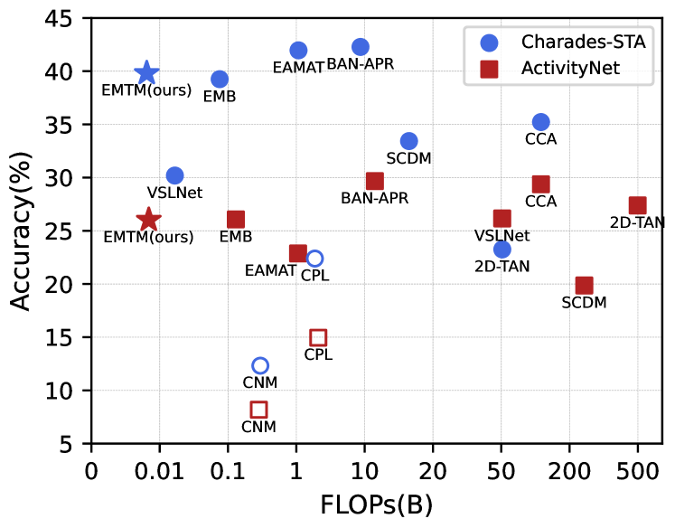
(a)

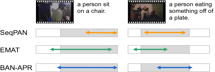
(b)

Figure 1. (a) FLOPs and accuracy plot of state-of-the-art TSGV approaches on Chradas-STA and ActivityNet. We report R1@0.7 for the two datasets. Our proposed EMTM achieves the best accuracy-speed balance among all the competitors. (b) Various predictions from different models when given the same input. Ground truth is shown in the gray area.

Temporal Sentence Grounding in Videos (TSGV), which aims to ground a temporal segment in an untrimmed video with a natural language query, has drawn widespread attention over the past few years (Zhang et al., 2023). There is a clear trend that top-performing models are becoming larger with numerous parameters. Additionally, the recent work shows that accuracy in TSGV tasks has reached a bottleneck period, while the combination of complex networks and multiple structures is becoming more prevalent to further improve the ability of the model, which will cause an expansion of the model size. However, the heavy resource cost required by the approaches restricts their applications to platforms and devices with limited computational capability and low memory storage.

In order to improve efficiency, FMVR (Gao and Xu, 2021) and CCA (Wu et al., 2022) are proposed to construct fast TSGV models by reducing the fusion time. Although they decline the inferred time significantly, the whole network is still time-consuming, even surpassing the conventional methods, as depicted in Figure 1(a). The time of the whole network encompasses the duration from inputting the video feature (e.g., I3D or C3D) and query sentence to producing predictions in this paper. To be specific, FMVR and CCA require encoding and storing of the video feature in advance, followed by inference based on the query. However, the encoding process is highly time-consuming. In real-world scenarios, there may not be an opportunity to pre-encode the video. The processing of their methods is more similar to the Video Corpus Moment Retrieval (VCMR), e.g. retrieval moment from an existing video corpus by a query. Our objective is to expand the efficiency interval to cover the entire TSGV model.

To tackle this challenge, the natural approach is to reduce the complexity of the network, which can involve decreasing the hidden dimension, reducing the number of layers, and eliminating auxiliary losses. Nevertheless, all of these methods will lead to a decrease in performance to some extent. One promising technique is knowledge distillation (Hinton et al., 2015) to mitigate the decrease in performance and maintain high levels of accuracy when lighting the network. Initially, knowledge distillation employed a single teacher, but as technology advanced, multiple teachers have been deemed beneficial for imparting greater knowledge(Fukuda et al., 2017), as extensively corroborated in other domains(Wang and Yoon, 2021). Multi-teacher strategy implies that there is a more diverse range of dark knowledge to be learned, with the optimal knowledge being more likely to be present (You et al., 2017). Regarding the TSGV task, different models will predict results with varying quality when given the same input, as shown in Figure 1(b). Thus far, multiple-teacher knowledge distillation has not been studied and exploited for the TSGV task.

An immediate problem is that different models will produce heterogeneous output, e.g., candidates for proposed methods, or probability distribution for proposal-free methods. Another question is how to identify optimal knowledge from multiple teachers. In addition, knowledge can hardly backpropagate to the front layers from the soft label in the last layers (Romero et al., 2014), meaning that the front part of the student model usually hardly enjoys the benefit of teachers’ knowledge. Until now, here are three issues we need to deal with: i) how to unify knowledge from the heterogeneous models, ii) how to select the optimal knowledge and assign weights among these teachers, and iii) how the front layers of the student benefit from the teachers.

Firstly, We unify the various types of outputs from multiple heterogeneous models into 1D probability distribution through corresponding processing. This enables us to seamlessly integrate the knowledge when training model. The 1D probability distribution is the output of the span-based method from the proposal-free catalog, which has an inherent speed advantage over the proposal-based methods. Then, a Knowledge Aggregation Unit (KAU) is built that associates the knowledge from the different models. KAU, which consists of multiple parallel transformations with different receptive fields, leverages multi-scale information(Li et al., 2021), thus obtaining target distribution with higher quality instead of simply averaging these probabilities. It adaptively determines the importance weights of different teachers with respect to a specific instance based on both the teacher and student representation, avoiding turning the weights of different teachers manually, which are sensitive hyperparameters for multiple teachers’ distillation (Liu et al., 2022a). Finally, a shared layer strategy was designed to learn shallow knowledge from the teacher. Specifically, an isomorphic teacher is added and co-trained with our student model while sharing their encoder layers and aligning their hidden states, which guarantees that the student is able to gain global and exhaustive knowledge.

Through the above approach, the whole student model is required to learn from both the isomorphic and heterogeneous teachers which serve as complementary cues to provide an enhanced supervisory signal when model training. During inference, we only exploit the student model to perform inference, which does not add computational overhead. To sum up, this paper’s primary contributions can be distilled into three main points, which are outlined below:

• We propose a multi-teacher knowledge distillation framework for the TSGV task. This approach substantially reduces the time consumed and significantly decreases the number of parameters, while still maintaining high levels of accuracy.

• To enable the whole student to benefit from various teacher models, we unify the knowledge from different models and use the KAU module to adaptively integrate to a single soft label. Additionally, a shared encoder strategy is utilized to share knowledge from the isomorphic teacher model in front layers.

• Extensive experimental results on three popular TSGV benchmarks demonstrate that our proposed method performs superior to the state-of-the-art methods and has the highest speed and minimal parameters and computation.

2. Related Work

Given an untrimmed video, temporal sentence grounding in videos (TSGV) is to retrieve a video segment according to a query, which is also known as Video Moment Retrieval (VMR). Existing solutions to video grounding are roughly categorized into proposal-based and proposal-free frameworks. We also introduce some works on fast video temporal grounding as follows.

2.1. Proposal-based Methods

The majority of proposal-based approaches rely on a number of carefully thought-out dense sample strategies, which gather a set of video segments as candidate proposals and rank them in accordance with the scores obtained for the similarity between the proposals and the query to choose the most compatible pairs. Yuan et al. (2019) offer a Semantic Conditioned Dynamic Modulation (SCDM) based on (Gao et al., 2017), which can combine the query with visual representations for correlating the sentence-related video contents and dynamically change the temporal convolution according to the query semantics. In order to produce excellent video temporal candidates, Xiao et al. (2021) propose a Boundary Proposal Network (BPN) using a third party model. Liu et al. (2022b) creat the Motion-Appearance Reasoning Network (MARN), which makes use of retrieved object information and models their relationships for improved localization, to differentiate frame-level features in videos. Rich temporal information is also taken into account in some works. Zhang et al. (2020a) convert visual features into a 2D temporal map and encode the query in sentence-level representation, which is the first solution to model proposals with a 2D temporal map (2D-TAN). BAN-APR (Dong and Yin, 2022) utilize a boundary-aware feature enhancement module to enhance the proposal feature with its boundary information by imposing a new temporal difference loss. Currently, most proposal-based methods are time-consuming due to the large number of proposal-query interactions.

2.2. Proposal-free Methods

Actually, the caliber of the sampled proposals has a significant impact on the impressive performance obtained by proposal-based methods. To avoid incurring the additional computational costs associated with the production of proposal features, proposal-free approaches directly regress or forecast the beginning and end times of the target moment. Wang et al. (2020) aggregate contextual information by obtaining the relations between the current segment and its neighbor segments and propose a Contextual Boundary-aware Prediction (CBP). VSLNet Zhang et al. (2020b) exploits context-query attention modified from QANet Yu et al. (2018) to perform fine-grained multimodal interaction. Then a conditioned span predictor computes the probabilities of the start/end boundaries of the target moment. SeqPAN (Zhang et al., 2021) design a self-guided parallel attention module to effectively capture self-modal contexts and cross-modal attentive information between video and text inspired by sequence labeling tasks in natural language processing. Yang and Wu (2022) propose Entity-Aware and Motion-Aware Transformers (EAMAT) that progressively localize actions in videos by first coarsely locating clips with entity queries and then finely predicting exact boundaries in a shrunken temporal region with motion queries. In addition, Huang et al. (2022) introduce Elastic Moment Bounding (EMB) to accommodate flexible and adaptive activity temporal boundaries toward modeling universally interpretable video-text correlation with tolerance to underlying temporal uncertainties in pre-fixed annotations. Nevertheless, with the improvement of performance, huge and complex architectures inevitably result in higher computational cost during inference phase.

2.3. Fast Video Temporal Grounding

Recently, fast video temporal grounding has been proposed for more practical applications. TSGV task usually requires methods to efficiently localize target video segments in thousands of candidate proposals. In fact, several early algorithms, e.g., common space-learning methods and scanning-based methods, make some contributions to reducing the computational costs. According to (Gao and Xu, 2021), the standard TSGV pipeline can be divided into three components. The visual encoder and the text encoder are proved to have little influence in model testing due to the features pre-extracted and stored at the beginning of the test, and cross-modal interaction is the key to reducing the test time. Thus, a fine-grained semantic distillation framework is utilized to leverage semantic information for improving performance. Besides, Wu et al. (2022) utilize commonsense knowledge to obtain bridged visual and text representations, promoting each other in common space learning. However, based on our previous analysis, the inferred time proposed by (Gao and Xu, 2021) is only a part of the entire prediction processing. The processing from inputting video features to predicting timestamps is still time-consuming.

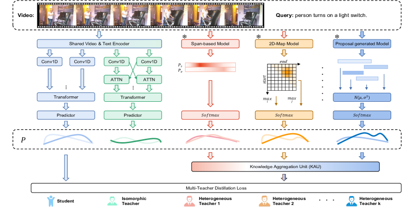
Figure 2. An overview of the proposed framework. EMTM mainly consists of three components: the student model, the shared encoder, and the KAU. The shared encoder with isomorphic structures is utilized to align their hidden states. Heterogeneous model outputs are unified into 1D probability distribution as shown in the right. Then it is adopted to adaptively determine the importance weights of different teachers with respect to a specific instance based on both the teacher and student representation. During the inference stage, only student model is adopted for fast TSGV.

3. Methodology

In this section, we first give a brief task definition of TSGV in Section 3.1. In the following, heterogeneous knowledge unification is presented as a prerequisite in Section 3.2.1. Then we introduce the student network (Section 3.2.2), shared encoder strategy (Section 3.2.4) and knowledge aggregation unit (Section 3.2.3) as shown in 2. Finally, the training and inference processes are presented in section 3.3, as well as the loss settings.

3.1. Problem Formulation

Given an untrimmed video $V=[f_{t}]_{t=1}^{T}$ and the language query $Q=[q_{j}]_{j=1}^{m}$, where $T$ and $m$ are the numbers of frames and words, respectively. The start and end times of the ground truth moment are indicated by $\tau^{s}$ and $\tau^{e}$, $1\leq\tau_{s}<\tau_{e}\leq T$. Mathematically, TSGV is to retrieve the target moment starting from $\tau_{s}$ and ending at $\tau_{e}$ by giving a video $V$ and query $Q$, i.e., $\mathcal{F}_{TSGV}:(V,Q)\mapsto(\tau_{s},\tau_{e})$.

3.2. General Scheme

3.2.1. Heterogeneous Knowledge Unification

Compared to the proposal-based method, the span-based method doesn’t need to generate redundant proposals, which is an inherent advantage in terms of efficiency. Meanwhile, 1D distribution carries more knowledge than the regression-based method. Hence we unify various heterogeneous outputs into 1D probability distribution and develop our network based on the span-based method, as shown in Figure 2. The outputs of the span-based method are the 1D probability distributions of start and end moments, denoted as $P_{s},P_{e}\in\mathbb{R}^{n}$. To keep concise, we adopt $P\in\mathbb{R}^{2n}$ without subscripts to express stacked probability for the start and end moments.

We simply adopt the softmax function to the outputs of the span-based methods and obtain probability distributions.

(1) $$P_{s}=Softmax(P^{\prime}_{s})\quad P_{e}=Softmax(P^{\prime}_{e})$$

2D-map anchor-based method is a common branch of the proposal-base method, such as (Zhang et al., 2020a), (Dong and Yin, 2022). A 2D map $S=[s_{i,j}]\in\mathbb{R}^{n\times n}$ is generated to model temporal relations between proposal candidates, on which one dimension indicates the start moment and the other indicates the end moment. We calculate the max scores of $S$ by row/column as start/end distributions.

(2) $$P_{s}= Softmax(\max\limits_{j}s_{i,j})$$

$$P_{e}= Softmax(\max\limits_{i}s_{i,j})$$

As for the regression-based method, we can get a time pair $(t_{s},t_{e})$ after computation. Then the Gaussian distribution is leveraged to simulate the probability distribution of the start/end moments as follows:

(3) $$P_{s}= Softmax({N(t_{s},\sigma^{2})})$$

$$P_{e}= Softmax({N(t_{e},\sigma^{2})})$$

The proposal-generated method will generate a triple candidate list $S^{\prime}=(t_{s}^{i},t_{e}^{i},r^{i})\in\mathbb{R}^{3\times k}$, where $k$ is the number of proposal candidates. Similarly, we use the Gaussian distribution to generate the probability distribution of the start/end moment for each candidate. Then we put different weights on various candidates and accumulate them:

(4) $$P_{s}= Softmax(\sum_{i}r^{i}{N(t_{s}^{i},\sigma^{2})})$$

$$P_{e}= Softmax(\sum_{i}r^{i}{N(t_{e}^{i},\sigma^{2})})$$

where $\sigma^{2}$ is the variance of Gaussian distribution $N$.

3.2.2. Student Network

For each video, we extract its visual features $\bm{V}\in\mathbb{R}^{n\times d_{v}}$ with a pre-trained convolutional neural network model (Carreira and Zisserman, 2017), where $n$ is the length of extracted features. For each query $Q$, we initialize the word features $\bm{Q}\in\mathbb{R}^{m\times d_{q}}$ by GloVe embeddings.

We first project $\bm{V}$ and $\bm{Q}$ into the same dimension $d$ by projection matrices, and incorporate a position embedding to every input of both video and query sequences. Then we feed the results into the $\mathtt{VisualEncoder}$ and $\mathtt{QueryEncoder}$ respectively:

(5) $$\bm{V^{\prime}} =\mathtt{VisualEncoder}(\mathtt{FFN_{v}}(\bm{V})+E_{p})$$

$$\bm{Q^{\prime}} =\mathtt{QueryEncoder}(\mathtt{FFN_{q}}(\bm{Q})+E_{p})$$

where $\mathtt{FFN}$ is projection matrices, $E_{p}$ denotes the positional embeddings. $\mathtt{VisualEncoder}$ and $\mathtt{QueryEncoder}$ consist of stacked 1D convolutional blocks to learn representations by carrying knowledge from neighbor tokens.

To enhance the cross-modal interactions between visual and textual features, we utilize the context-query attention (CQA) strategy  (Lu et al., 2019), and aggregate text information for each visual element. Specially, we calculate the similarity scores $\mathcal{S}\in\mathbb{R}^{n\times m}$ between each visual feature and query feature. Then the attention weights of visual-to-query ($\mathcal{A}$) and query-to-visual ($\mathcal{B}$) are computed as:

(6) $$\mathcal{A} =\mathcal{S}_{r}\cdot\bm{Q^{\prime}}\in\mathbb{R}^{n\times d}$$

$$\mathcal{B} =\mathcal{S}_{r}\cdot\mathcal{S}_{c}^{T}\cdot\bm{V^{\prime}}\in\mathbb{R}^{n\times d}$$

where $\mathcal{S}_{r}$ and $\mathcal{S}_{c}$ are the row-wise and column-wise normalization of $\mathcal{S}$ by softmax operation, respectively. Finally, the output of visual-query attention is written as:

(7) $$\bm{V}^{qv}=\mathtt{FFN}\big{(}[\bm{V^{\prime}};\mathcal{A};\bm{V^{\prime}}\odot\mathcal{A};\bm{V^{\prime}}\odot\mathcal{B}]\big{)}$$

where $\bm{V}^{qv}\in\mathbb{R}^{n\times d}$; $\mathtt{FFN}$ is a single feed-forward layer; $\odot$ denotes element-wise multiplication. $\bm{V}^{qv}$ is the fused multi-modal semantic features with visual and query attention. Then we follow (Zhang et al., 2021) and calculate $\bm{P_{s}}$ and $\bm{P_{e}}$. Hence, the prediction part of TSGV model can be defined as:

(8) $$(\bm{P_{s}},\bm{P_{e}})=\mathtt{Predictor}(\bm{V^{qv}})\in\mathbb{R}^{n}$$

Method Year Charades-STA ActivityNet TACoS FLOPS (B) Params (M) Times (ms) sumACC FLOPS (B) Params (M) Times (ms) sumACC FLOPS (B) Params (M) Times (ms) sumACC SCDM 2019 16.5000 12.8800 - 87.87 260.2300 15.6500 - 56.61 260.2300 15.6500 - - 2D-TAN 2020 52.2616 69.0606 13.3425 66.05 1067.9000 82.4400 77.9903 71.43 1067.9000 82.4400 77.9903 *36.82 VSLNet 2020 0.0300 0.7828 8.0020 77.50 0.0521 0.8005 8.9893 69.38 0.0630 0.8005 8.9893 44.30 SeqPAN 2021 0.0209 1.1863 10.5168 102.20 0.0214 1.2143 13.7138 73.87 0.0218 1.2359 23.3025 67.71 EMB 2022 0.0885 2.2168 22.3900 97.58 0.2033 6.1515 25.0871 70.88 0.2817 2.2172 23.6349 60.36 EAMAT 2022 1.2881 94.1215 56.1753 103.65 4.1545 93.0637 125.7822 60.94 4.1545 93.0637 125.7822 64.98 BAN-APR 2022 9.4527 34.6491 19.9767 105.96 25.4688 45.6714 44.8587 77.79 25.4688 45.6714 44.8587 *52.10 CPL 2022 3.4444 5.3757 26.8451 71.63 3.8929 7.0115 26.4423 49.14 - - - - CNM 2022 0.5260 5.3711 5.4482 50.10 0.5063 7.0074 4.8629 *48.96 - - - - FVMR 2021 - - - 88.75 - - - 71.85 - - - - CCA 2022 137.2984 79.7671 26.9734 89.41 151.1023 22.5709 31.5400 *75.95 151.1023 22.5709 31.5400 50.90 EMTM (Ours) 0.0081 0.6569 4.7998 92.80 0.0084 0.6848 3.5431 70.91 0.0087 0.7065 4.5737 58.24

Table 1. Efficiency analysis on Charades-STA, ActivityNet, and TACoS. sumACC is the sum of R1@0.5 and R1@0.7. All the data is measured with strict adherence to the source code in the same environment. * denotes the accuracy we reproduce.

3.2.3. Knowledge Aggregation Unit

Our goal is to combine all the unified predictions from $b$ branches to establish a strong teacher distribution. Previous image classification work (Zhu et al., 2018) adopted a simple convolution block as the gate module to generate an importance score for each branch. But a simple convolution block cannot effectively capture the contextual representation due to the temporal scale variation problem which widely exists in video tasks. Thus, capturing multi-scale information is required to handle this problem. Inspired by the previous works (Li et al., 2021), we design the Knowledge Aggregation Unit (KAU), which consists of multiple parallel transformations with different receptive fields, leveraging both local and global information to obtain a more accurate target probability. The architecture of the proposed KAU is depicted in Figure 3.

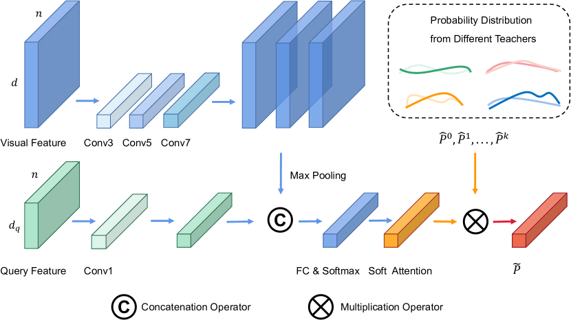
Figure 3. Illustration of Knowledge Aggregation Unit, which exploits the multi-scale information from various teachers to generate higher-quality knowledge. The final ensemble probability distribution $\widetilde{P}$ is obtained by the weighted sum from all individual branches.

Considering saving more original information, we first take the video features $V^{\prime}$ in the eq. (5) as input and then add convolution layers. The convolution operation is conducted with a small kernel size of 3 initially and then consistently increased to 5 and 7.

Further, we incorporate the average pooling of query features $Q^{\prime}$ in the eq. (5) for richer representations. Then we concatenate all the splits and obtain the intermediate vector $v$, denoted as:

(9) $$v=[q_{avg},g([v_{conv3},v_{conv5},v_{conv7}])]$$

where $q_{avg}$ denotes the result of $Q^{\prime}$ after average pooling, g(·) denotes the global pooling function, $v_{conv3}$, $v_{conv5}$, and $v_{conv7}$ denote the results after the convolution layers with kernel size 3, 5, and 7, respectively.

Passing through a fully connected layer $FC$, a channel-wise softmax operator is applied to obtain the soft attention $a$.

(10) $$a=Softmax(\mathtt{FC}(v))\in\mathbb{R}^{2b\times n}$$

where the $b$ denote the number of teacher branch, $2b$ is because there are two probability distributions (i.e., start and end).

Finally, we fuse prediction results from multiple branches via an element-wise summation to obtain the weighted ensemble probability.

(11) $$\widetilde{P}=\sum_{i=1}^{b}{a^{i}\otimes\hat{P}^{i}}\in\mathbb{R}^{2\times n}$$

where $\widetilde{P}$ denotes the ensemble probability, $P^{i}\in\mathbb{R}^{2\times n}$ means the start and end distribution from $i$-th teacher branch, and $\otimes$ refers to the channel-wise multiplication. Our experiments (see Section 4.5.1) prove that the weights generated by KAU can achieve better distillation performance.

3.2.4. Shared Encoder Strategy

When the knowledge that exists in soft label backpropagates from back to front, the shallow layers hardly enjoy the benefit, due to the non-linear activity function and dropout design. But the feature invariant in the shallow layers (Zeiler and Fergus, 2014) inspires us, we share several shallow layers of the student with an isomorphic teacher. Through collaborative training with the teacher network, the shallow layers can acquire additional knowledge.

Specifically, a student and an isomorphic teacher share their text and query encoder, shown in Figure 2. The encoder consists of several conv1D in our network, which is lightweight and fast due to its inherent characteristic. The $\mathtt{VisualEncoder}$, $\mathtt{QueryEncoder}$, and $\mathtt{FFN}$ layers in eq. (5) denote the shared layers in our network.

3.3. Training and Inference

3.3.1. TSGV Loss

The overall training loss of our model is described as follows. For the student and the isomorphic teacher, the hard loss (i.e. label loss) is used to optimize distributions of start/end boundaries.

(12) $$L^{st}_{loc}=f_{CE}(P^{st},Y)$$

$$L^{tc}_{loc}=f_{CE}(P^{tc},Y)$$

where $f_{CE}$ is the cross-entropy function, and $Y$ is one-hot labels for the start and end boundaries of ground truth. Similarly, we encourage ensemble probability to get closer to ground truth distribution.

(13) $$L^{ens}_{loc}=f_{CE}(\widetilde{P},Y)$$

As we discussed previously, the learned ensemble information serves as complementary cues to provide an enhanced supervisory signal to our student model. As a result, we introduce multiple distillation learning, which transfers the rich knowledge in the form of softened labels. The formulation is given by:

(14) $$L_{dis}=f_{KL}(softmax(P^{st},t),softmax(\widetilde{P},t)$$

where $f_{KL}$ represents the KL divergence. The $t$ is the temperature in knowledge distillation, which control the smoothness of the output distribution.

Based on the above design, the overall objective for a training video-query pair is formulated as:

(15) $$L=L^{st}_{loc}+L^{tc}_{loc}+L^{ens}_{loc}+\alpha L_{dis}$$

where $\alpha$ is a balance term.

3.3.2. Inference

The teacher and student models will be collaboratively trained, while we only adopt the student model for TSGV during testing. The learned rich information serves as complementary cues to provide an enhanced supervisory signal to the TSGV model. Compared with FMVR (Gao and Xu, 2021) and CCA (Wu et al., 2022), we won’t pre-calculate and store visual features.

Method Charades-STA ActivityNet TACoS R1@0.3 R1@0.5 R1@0.7 mIoU R1@0.3 R1@0.5 R1@0.7 mIoU R1@0.3 R1@0.5 R1@0.7 mIoU SCDM - 54.44 33.43 - 54.80 36.75 19.86 - 26.11 21.17 - - 2D-TAN - 42.80 23.25 - 58.75 44.05 27.38 - 35.17 25.17 11.65 24.16 VSLNet 64.30 47.31 30.19 45.15 63.16 43.22 26.16 43.19 29.61 24.27 20.03 24.11 SeqPAN 73.84 60.86 41.34 53.92 61.65 45.50 28.37 45.11 48.64 39.64 28.07 37.17 EMB 72.50 58.33 39.25 53.09 64.13 44.81 26.07 45.59 50.46 37.82 22.54 35.49 EAMAT 74.19 61.69 41.96 54.45 55.33 38.07 22.87 40.12 50.11 38.16 26.82 36.43 BAN-APR *74.05 63.68 42.28 *54.15 *65.11 48.12 29.67 *45.87 48.24 33.74 *17.44 *32.95 CPL 66.40 49.24 22.39 43.48 55.73 31.37 12.32 36.82 - - - - CNM 60.04 35.15 14.95 - 55.68 33.33 *12.81 * 36.15 - - - - FVMR - 55.01 33.74 - 60.63 45.00 26.85 - 41.48 29.12 - - CCA 70.46 54.19 35.22 50.02 61.99 46.58 29.37 *45.11 45.30 32.83 18.07 - EMTM (Ours) 72.70 57.91 39.80 53.00 63.20 44.73 26.08 45.33 45.78 34.83 23.41 34.44 $\Delta_{SOTA}$ $\uparrow$ 2.24 $\uparrow$ 2.90 $\uparrow$ 4.58 $\uparrow$ 2.98 $\uparrow$ 1.21 $\downarrow$ 1.85 $\downarrow$ 3.29 $\uparrow$ 0.22 $\uparrow$ 0.48 $\uparrow$ 2.42 $\uparrow$ 5.34 -

Table 2. Performance comparison with the state-of-the-art methods.

4. Experiments

4.1. Datasets

To evaluate the performance of TSGV, we conduct experiments on three challenging video moment retrieval datasets, all the queries in these datasets are in English. Details of these datasets are shown as follows:

Charades-STA (Gao et al., 2017) is composed of daily indoor activities videos, which is based on Charades dataset (Sigurdsson et al., 2016). This dataset contains 6672 videos, 16,128 annotations, and 11,767 moments. The average length of each video is 30 seconds. $12,408$ and $3,720$ moment annotations are labeled for training and testing, respectively;

ActivityNet Caption (Caba Heilbron et al., 2015) is originally constructed for dense video captioning, which contains about $20$k YouTube videos with an average length of 120 seconds. As a dual task of dense video captioning, video moment retrieval utilize the sentence description as a query and outputs the temporal boundary of each sentence description.

TACoS (Regneri et al., 2013) is collected from MPII Cooking dataset (Regneri et al., 2013), which has 127 videos with an average length of $286.59$ seconds. TACoS has 18,818 query-moment pairs, which are all about cooking scenes. We follow the same splits in (Gao et al., 2017), where $10,146$, $4,589$, and $4,083$ annotations are used for training, validation, and testing, respectively.

4.2. Evaluation Metrics

Following existing video grounding works, we evaluate the performance on two main metrics:

mIoU: “mIoU" is the average predicted Intersection over Union in all testing samples. The mIoU metric is particularly challenging for short video moments;

Recall: We adopt “$\textrm{R@}n,\textrm{IoU}=\mu$” as the evaluation metrics, following (Gao et al., 2017). The “$\textrm{R@}n,\textrm{IoU}=\mu$” represents the percentage of language queries having at least one result whose IoU between top-$n$ predictions with ground truth is larger than $\mu$. In our experiments, we reported the results of $n=1$ and $\mu\in\{0.3,0.5,0.7\}$.

The Metric of Efficiency: Time, FLOPs, and Params are used to measure the efficiency of the model. Specifically, the time refers to the entire inferring time from the input of the video and query pair to the output of the prediction. FLOPs refers to floating point operations, which is used to measure the complexity of the model. Params refers to the model parameter size except the word embedding.

4.3. Implementation Details

For language query $Q$, we use the $300$-D GloVe (Pennington et al., 2014) vectors to initialize each lowercase word, which are fixed during training. Following the previous methods, 3D convolutional features (I3D) are extracted to encode videos. We set the dimension of all the hidden layers as $128$, the kernel size of the convolutional layer as $7$, and the head size of multi-head attention as $8$ in our model. For all datasets, models are trained for $100$ epochs. The batch size is set to $16$. The dropout rate is set as 0.2. Besides, an early stopping strategy is adopted to prevent overfitting. The whole framework is trained by Adam optimizer with an initial learning rate of 0.0001. The loss weight $\alpha$ is set as 0.1 in all the datasets. The temperate was set to 1, 3, 3 on Charades-STA, ActivityNet, and TACoS. The pre-trained teacher models are selected in SeqPAN, BAN-APR, EAMAT, and CCA, and we use SeqPAN as an isomorphic teacher to share the encoder. More ablation studies can be found in Section 4.5. All experiments are conducted on an NVIDIA RTX A5000 GPU with 24GB memory. All experiments were performed three times, and reporting the average of performance.

4.4. Comparison with State-of-the-art Methods

We strive to gather the most current approaches, and compare our proposed model with the following state-of-the-art baselines on three benchmark datasets:

• Proposal-based Methods: SCDM (Yuan et al., 2019), 2D-TAN (Zhang et al., 2020a), BAN-APR (Dong and Yin, 2022).

• Proposal-free Methods: VSLNet (Zhang et al., 2020b), SeqPAN (Zhang et al., 2021), EMB (Huang et al., 2022), EAMAT (Yang and Wu, 2022).

• Weakly Supervised Methods: CPL (Zheng et al., 2022), CNM (Zheng et al., 2022)

• Fast Methods: FVMR (Gao and Xu, 2021), CCA (Wu et al., 2022)

The best performance is highlighted in bold and the second-best is highlighted with underline in tables.

Overall Efficiency-Accuracy Analysis

Considering that fast TSGV task pays the same attention to the efficiency as the accuracy, we evaluate FLOPs, Params, and Times for each model. For a fair comparison, the batch size is set to 1 for all methods during inference. Besides, we also calculate the sum of the accuracy in terms of “R1@0.3” and “R1@0.5”, named sumACC to evaluate the whole performance of each model.

As Table 1 shows, our method surpasses all other methods and achieves the highest speed, minimal FLOPs and Params on all three datasets. We can find that our proposed method is at least 2000 times fewer in FLOPs than state-of-the-arts proposal-based models (SCDM and 2D-TAN). According to sumACC, we also notice that our proposed EMTM outperforms these two models by gains of at most 26.75% on Charades-STA and 14.30% on ActivtyNet. Though these proposal-free approaches such as VSLNet, SeqPAN and EMB also achieve favorable performance with low computational expenses, our proposed method still outperforms better overall. Compared to the baseline method SeqPAN, although there is a slight accuracy decrease, we achieve 4x fewer in FLOPs and 2x faster. Despite the parameter size of VSLNet is at the same level as our method, we outperform it significantly in terms of accuracy. For instance, EMTM achieves 15.30% absolute improvement by “sumACC” on Charades-STA. When it comes to CCA, which is proposed for fast TSGV, EMTM outperforms 16950x fewer in FLOPs and 121x fewer in model parameter size on Charades-STA. The above comparison illustrates that our method has significant efficiency and accuracy advantages.

Accuracy Analysis

We compare the performance of our proposed method against extensive video temporal grounding models on three benchmark datasets. As shown in Table 2, we can observe that our method performs better than other methods in most metrics. Compared with FVMR and CCA, our model performers better in all metrics. Especially, EMTM achieves an absolute improvement of 4.58% on Charades- STA and 5.34% on TACoS on the metric "R@1, IoU=0.7". Note that R@1, IoU=0.7 is a more crucial criterion to determine whether a TSGV model is accurate or not. The comparison of performance "on R1, IoU=0.7" shows that our method can predict results with higher quality.

Then, we compare our model with much more TSGV methods in more detail. Firstly, we compare EMTM with previous proposal-based methods: SCDM and 2D-TAN. From the results in Table 2, we observe that our EMTM achieves great performance compared with the aforementioned methods on most of the metrics. We also notice that EMTM surpasses 2D-TAN on Charades-STA and TACoS by (16.55%, 11.76%) in terms of “R@1, IoU=0.7”. Moreover, we compare our method with previous proposal-free methods: VSLNet, SeqPAN, EMB and EAMAT. Compared with them, our proposed CCA method achieves better performance. On ActivityNet, we outperform VSLNet by gains of (1.51%, 2.14%) in terms of “R@1, IoU=0.5” and "mIoU". Besides, it also surpasses the recent work EAMAT with an average 7.22% improvement on the metrics “R@1, IoU=0.3, 0.5, 0.7”. ActivtyNet has larger scales than the other two datasets. The results indicate that our method also performs well in a more complex visual-text environment. In addition, our model offers apparent benefits over weakly supervised methods. It indicates that our method can localize the moment with higher quality. Our EMTM obtains more accurate results because multiple teachers make the model have the ability to comprehend complex cross-modal relationships. In fact, the simple but effective use of transferred knowledge replaces large and repetitive cross-modal interaction and reduces the time and computational cost. It validates that EMTM can efficiently and effectively localize the target moment boundary.

Method Shared Encoder Label Distillation R1@0.3 R1@0.5 R1@0.7 mIoU EMTM w/o SE-LD ✗ ✗ $70.19_{{\color[rgb]{0,0,1}-0.99}}^{{\color[rgb]{1,0,0}+0.97}}$ $56.23_{{\color[rgb]{0,0,1}-1.01}}^{{\color[rgb]{1,0,0}+0.62}}$ $36.49_{{\color[rgb]{0,0,1}-0.74}}^{{\color[rgb]{1,0,0}+0.39}}$ $51.34_{{\color[rgb]{0,0,1}-1.06}}^{{\color[rgb]{1,0,0}+0.98}}$ EMTM w/o SE ✗ ✔ $\textbf{73.33}_{{\color[rgb]{0,0,1}-1.34}}^{{\color[rgb]{1,0,0}+0.84}}$ $\textbf{58.05}_{{\color[rgb]{0,0,1}-0.25}}^{{\color[rgb]{1,0,0}+0.26}}$ $\underline{38.36}_{{\color[rgb]{0,0,1}-0.21}}^{{\color[rgb]{1,0,0}+0.17}}$ $\textbf{53.31}_{{\color[rgb]{0,0,1}-0.91}}^{{\color[rgb]{1,0,0}+0.54}}$ EMTM w/o LD ✔ ✗ $72.62_{{\color[rgb]{0,0,1}-0.52}}^{{\color[rgb]{1,0,0}+0.69}}$ $56.51_{{\color[rgb]{0,0,1}-0.84}}^{{\color[rgb]{1,0,0}+1.18}}$ $37.54_{{\color[rgb]{0,0,1}-0.50}}^{{\color[rgb]{1,0,0}+0.85}}$ $52.39_{{\color[rgb]{0,0,1}-0.37}}^{{\color[rgb]{1,0,0}+0.60}}$ EMTM ✔ ✔ $\underline{72.70}_{{\color[rgb]{0,0,1}-0.55}}^{{\color[rgb]{1,0,0}+0.47}}$ $\underline{57.91}_{{\color[rgb]{0,0,1}-0.65}}^{{\color[rgb]{1,0,0}+0.75}}$ $\textbf{39.80}_{{\color[rgb]{0,0,1}-0.12}}^{{\color[rgb]{1,0,0}+0.12}}$ $\underline{53.00}_{{\color[rgb]{0,0,1}-0.33}}^{{\color[rgb]{1,0,0}+0.21}}$

Table 3. Effects of Main Components on Charades-STA.

Method Shared Encoder Label Distillation R1@0.3 R1@0.5 R1@0.7 mIoU EMTM w/o SE-LD ✗ ✗ $62.06_{{\color[rgb]{0,0,1}-0.85}}^{{\color[rgb]{1,0,0}+0.99}}$ $43.90_{{\color[rgb]{0,0,1}-0.39}}^{{\color[rgb]{1,0,0}+0.25}}$ $25.63_{{\color[rgb]{0,0,1}-0.13}}^{{\color[rgb]{1,0,0}+0.07}}$ $44.52_{{\color[rgb]{0,0,1}-0.38}}^{{\color[rgb]{1,0,0}+0.55}}$ EMTM w/o SE ✗ ✔ $\underline{63.19}_{{\color[rgb]{0,0,1}-0.22}}^{{\color[rgb]{1,0,0}+0.35}}$ $44.11_{{\color[rgb]{0,0,1}-0.27}}^{{\color[rgb]{1,0,0}+0.26}}$ $25.74_{{\color[rgb]{0,0,1}-0.32}}^{{\color[rgb]{1,0,0}+0.41}}$ $45.15_{{\color[rgb]{0,0,1}-0.03}}^{{\color[rgb]{1,0,0}+0.03}}$ EMTM w/o LD ✔ ✗ $62.98_{{\color[rgb]{0,0,1}-0.40}}^{{\color[rgb]{1,0,0}+0.33}}$ $\textbf{44.68}_{{\color[rgb]{0,0,1}-0.15}}^{{\color[rgb]{1,0,0}+0.19}}$ $\textbf{26.10}_{{\color[rgb]{0,0,1}-0.06}}^{{\color[rgb]{1,0,0}+0.12}}$ $\underline{45.22}_{{\color[rgb]{0,0,1}-0.12}}^{{\color[rgb]{1,0,0}+0.11}}$ EMTM ✔ ✔ $\textbf{63.20}_{{\color[rgb]{0,0,1}-0.58}}^{{\color[rgb]{1,0,0}+0.30}}$ $\underline{44.73}_{{\color[rgb]{0,0,1}-0.33}}^{{\color[rgb]{1,0,0}+0.58}}$ $\underline{26.08}_{{\color[rgb]{0,0,1}-0.31}}^{{\color[rgb]{1,0,0}+0.27}}$ $\textbf{45.33}_{{\color[rgb]{0,0,1}-0.31}}^{{\color[rgb]{1,0,0}+0.19}}$

Table 4. Effects of Main Components on ActivityNet

4.5. Ablation Studies

In this part, we perform in-depth ablation studies to analyze the effectiveness of the EMTM. All experiments are performed three times with different random seeds to eliminate the contingency.

4.5.1. Effects of Main Components

In our proposed framework, we design the sharing encoders (SE) to learn shallow knowledge from the isomorphic teacher, while knowledge contained in soft targets is taught by label distillation(LD). To better reflect the effects of these two main components, we measure the performance of different combinations. As table 3 and 4 show, each interaction component has a positive effect on the TSGV task. On Charades-STA, the full model outperforms w/o SE by gains of 1.44% on metrics “R@1, IoU=0.7” and exceeds “w/o LD” by (0.08%, 1.40%, 2.26%, 0.61%) on the all metrics. Besides, the full model also outperforms “w/o SE-LD” by a large margin on all metrics while achieving a significant 2.26% improvement in terms of “R@1, IoU=0.7”. Similarly, our full model has made significant improvements in every metric compared with the variant "EMTM w/o SE-LD" on ActivityNet.

Obviously, the interaction between sharing encoders and multiple teachers’ label distillation leads to a favorable improvement in performance, which proves that various teachers inject useful knowledge into our student model. As a result, the student model has become stronger than every teacher.

4.5.2. Effect of Number of Teacher Models

We investigate the influence of different numbers of teacher models on Charades-STA. As shown in 4, the performance presents a rising tendency with the increase of teachers. If SeqPAN is removed, the accuracy will be reduced by about 1% in terms of R1@0.7. When simply utilizing EAMAT, the performance will reach 38.25% and 52.69% compared to the original student 32.71% and 52.50% on mIoUR and 1@0.7, which proves the effectiveness of EAMAT. However, there exists a great distance of nearly 2% between our full model and its variant ’no teacher’, showing that one teacher is not enough. In summary, our improvements are not only from soft targets with one single teacher, but also from the learning of structural knowledge and intermediate-level knowledge with fused multi-teacher teaching. Multiple teachers make knowledge distillation more flexible, ensemble helps improve the training of student and transfer related information of examples to the student.

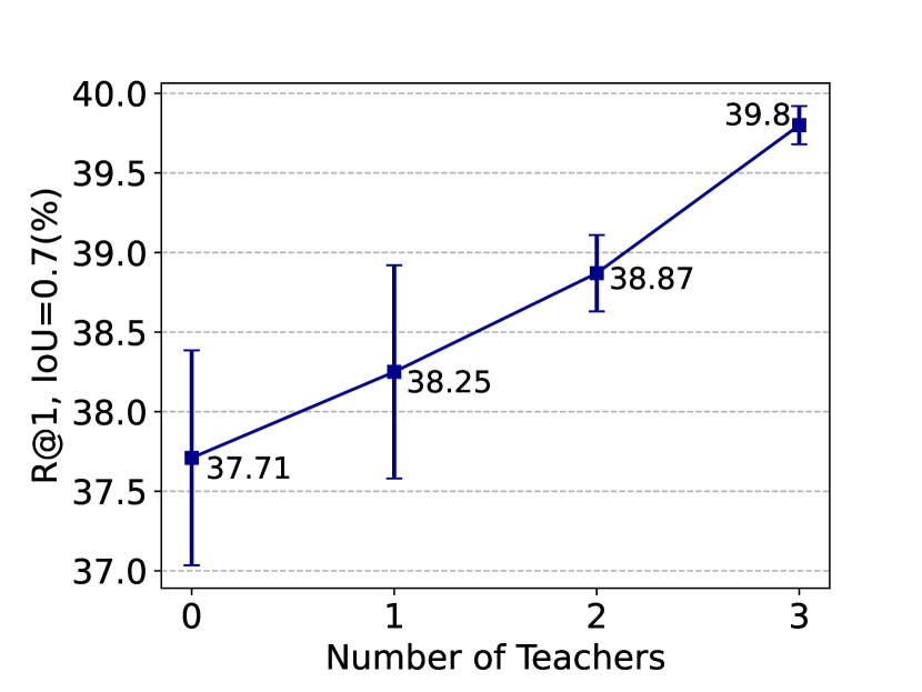
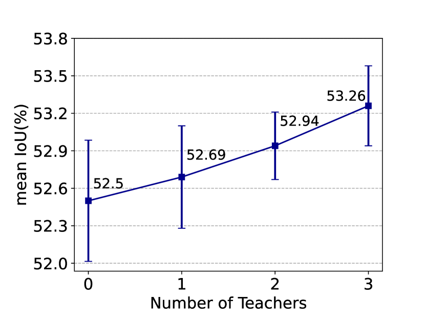
Figure 4. Effect of the Number of Teacher Models on Charades-STA. In detail, we adopt EAMAT, EAMAT & BAN-APR, EAMAT & BAN-APR & SeqPAN, which correspond to one teacher, two teachers and three teachers respectively.

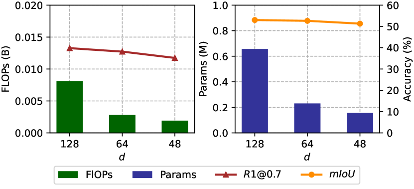
Figure 5. Effect of different degrees of lightweight by adjusting the hidden dimension $d$.

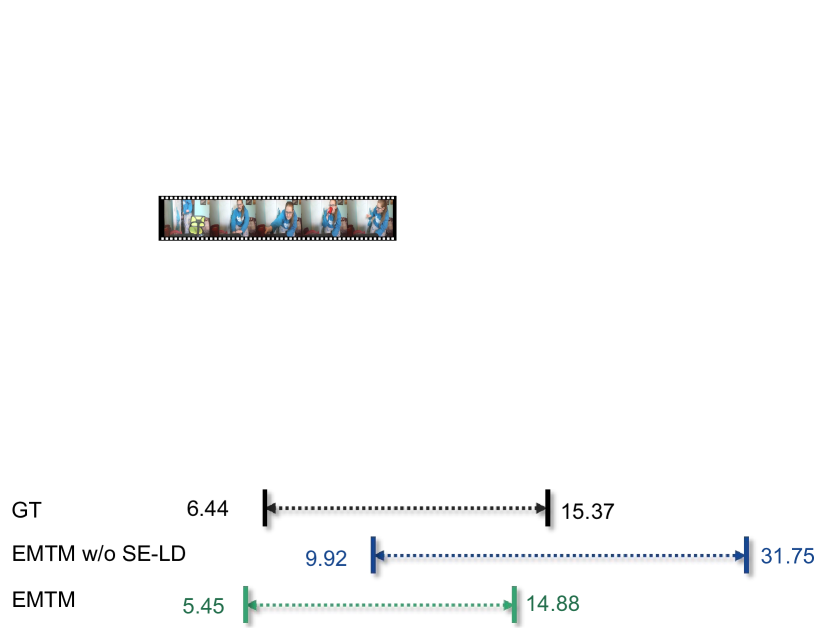
Figure 6. Examples of visualization of EMTM w/o SE-LD and EMTM on the Charades-STA.

4.5.3. Effect of Different Degree of Lightweight Models

We evaluate the influence of different degrees of lightweight models by adjusting their hidden dimension $d$ on Charades-STA. As shown in 5, obviously as $d$ decreases, the FLOPs and model parameter size will decline, which would also reduce the performance of our model. From 128 to 64 for $d$, both R1@0.7 and mIoU reduce by about 5%, while FLOPs and model parameter size drop by a small margin. For the trade-offs, we select 128 as the hidden dimension in our full model.

4.6. Qualitative Analysis

Two samples of prediction on Charades-STA are depicted in Figure 6. In general, the moments retrieved by full EMTM are closer to the ground truth than that are retrieved by EMEM without utilizing the shared encoder and label distillation strategy. The first sample indicated our approach can refine the predictions when the basic model already obtained satisfactory results. The second sample shows the basic model trend to predict the boundary position, possibly due to its limited understanding of the video. As a result, the model relies on biased positional information to make moment predictions. However, utilizing a shared encoder and label distillation approach can provide additional information that enables the model to more precisely predict the moment boundary.

5. Conclusion

In this paper, we focus on the efficiency of the model on Temporal Sentence Grounding in Videos and try to expand the efficiency interval to cover the entire TSGV model. A knowledge distillation framework (EMTM) is proposed, which utilizes label distillation from multiple teachers and a shared encoder strategy. We additionally design corresponding processes to unify heterogeneous outputs, enabling a smooth knowledge distillation in the subsequent step. Our model achieves high effectiveness and efficiency at the same time. The experimental results demonstrate that our method exhibits strong generalization.

In the future, we will pay attention to video feature extraction in TSGV, which is also a time-consume process. In real scenarios like surveillance video retrieval with raw videos as input, this issue is much more critical. We tend to explore the lightweight end-to-end model that includes the part of video feature extraction, thereby eliminating the constraints of computational capacity and high-demand storage.

References

- (1)
- Caba Heilbron et al. (2015) Fabian Caba Heilbron, Victor Escorcia, Bernard Ghanem, and Juan Carlos Niebles. 2015. Activitynet: A large-scale video benchmark for human activity understanding. In CVPR. 961–970.
- Carreira and Zisserman (2017) Joao Carreira and Andrew Zisserman. 2017. Quo vadis, action recognition? a new model and the kinetics dataset. In proceedings of the IEEE Conference on Computer Vision and Pattern Recognition. 6299–6308.
- Dong and Yin (2022) Jianxiang Dong and Zhaozheng Yin. 2022. Boundary-aware Temporal Sentence Grounding with Adaptive Proposal Refinement. In Proceedings of the Asian Conference on Computer Vision. 3943–3959.
- Fukuda et al. (2017) Takashi Fukuda, Masayuki Suzuki, Gakuto Kurata, Samuel Thomas, Jia Cui, and Bhuvana Ramabhadran. 2017. Efficient Knowledge Distillation from an Ensemble of Teachers.. In Interspeech. 3697–3701.
- Gao et al. (2017) Jiyang Gao, Chen Sun, Zhenheng Yang, and Ram Nevatia. 2017. Tall: Temporal activity localization via language query. In Proceedings of the IEEE international conference on computer vision. 5267–5275.
- Gao and Xu (2021) Junyu Gao and Changsheng Xu. 2021. Fast video moment retrieval. In Proceedings of the IEEE/CVF International Conference on Computer Vision. 1523–1532.
- Hinton et al. (2015) Geoffrey Hinton, Oriol Vinyals, and Jeff Dean. 2015. Distilling the knowledge in a neural network. arXiv preprint arXiv:1503.02531 (2015).
- Huang et al. (2022) Jiabo Huang, Hailin Jin, Shaogang Gong, and Yang Liu. 2022. Video Activity Localisation with Uncertainties in Temporal Boundary. In Computer Vision–ECCV 2022: 17th European Conference, Tel Aviv, Israel, October 23–27, 2022, Proceedings, Part XXXIV. Springer, 724–740.
- Li et al. (2021) Zheng Li, Jingwen Ye, Mingli Song, Ying Huang, and Zhigeng Pan. 2021. Online knowledge distillation for efficient pose estimation. In Proceedings of the IEEE/CVF International Conference on Computer Vision. 11740–11750.
- Liu et al. (2022b) Daizong Liu, Xiaoye Qu, Pan Zhou, and Yang Liu. 2022b. Exploring motion and appearance information for temporal sentence grounding. In Proceedings of the AAAI Conference on Artificial Intelligence, Vol. 36. 1674–1682.
- Liu et al. (2022a) Jihao Liu, Boxiao Liu, Hongsheng Li, and Yu Liu. 2022a. Meta knowledge distillation. arXiv preprint arXiv:2202.07940 (2022).
- Lu et al. (2019) Chujie Lu, Long Chen, Chilie Tan, Xiaolin Li, and Jun Xiao. 2019. DEBUG: A dense bottom-up grounding approach for natural language video localization. In EMNLP. 5147–5156.
- Pennington et al. (2014) Jeffrey Pennington, Richard Socher, and Christopher D Manning. 2014. Glove: Global vectors for word representation. In EMNLP. 1532–1543.
- Regneri et al. (2013) Michaela Regneri, Marcus Rohrbach, Dominikus Wetzel, Stefan Thater, Bernt Schiele, and Manfred Pinkal. 2013. Grounding action descriptions in videos. ACL 1 (2013), 25–36.
- Romero et al. (2014) Adriana Romero, Nicolas Ballas, Samira Ebrahimi Kahou, Antoine Chassang, Carlo Gatta, and Yoshua Bengio. 2014. Fitnets: Hints for thin deep nets. arXiv preprint arXiv:1412.6550 (2014).
- Sigurdsson et al. (2016) Gunnar A Sigurdsson, Gül Varol, Xiaolong Wang, Ali Farhadi, Ivan Laptev, and Abhinav Gupta. 2016. Hollywood in homes: Crowdsourcing data collection for activity understanding. In ECCV. 510–526.
- Wang et al. (2020) Jingwen Wang, Lin Ma, and Wenhao Jiang. 2020. Temporally grounding language queries in videos by contextual boundary-aware prediction. In Proceedings of the AAAI Conference on Artificial Intelligence, Vol. 34. 12168–12175.
- Wang and Yoon (2021) Lin Wang and Kuk-Jin Yoon. 2021. Knowledge distillation and student-teacher learning for visual intelligence: A review and new outlooks. IEEE Transactions on Pattern Analysis and Machine Intelligence (2021).
- Wu et al. (2022) Ziyue Wu, Junyu Gao, Shucheng Huang, and Changsheng Xu. 2022. Learning Commonsense-aware Moment-Text Alignment for Fast Video Temporal Grounding. arXiv preprint arXiv:2204.01450 (2022).
- Xiao et al. (2021) Shaoning Xiao, Long Chen, Songyang Zhang, Wei Ji, Jian Shao, Lu Ye, and Jun Xiao. 2021. Boundary proposal network for two-stage natural language video localization. In Proceedings of the AAAI Conference on Artificial Intelligence, Vol. 35. 2986–2994.
- Yang and Wu (2022) Shuo Yang and Xinxiao Wu. 2022. Entity-aware and Motion-aware Transformers for Language-driven Action Localization. In Proceedings of the Thirty-First International Joint Conference on Artificial Intelligence, LD Raedt, Ed. 1552–1558.
- You et al. (2017) Shan You, Chang Xu, Chao Xu, and Dacheng Tao. 2017. Learning from Multiple Teacher Networks. In Proceedings of the 23rd ACM SIGKDD International Conference on Knowledge Discovery and Data Mining (Halifax, NS, Canada) (KDD ’17). Association for Computing Machinery, New York, NY, USA, 1285–1294. https://doi.org/10.1145/3097983.3098135
- Yu et al. (2018) Adams Wei Yu, David Dohan, Quoc Le, Thang Luong, Rui Zhao, and Kai Chen. 2018. Fast and accurate reading comprehension by combining self-attention and convolution. In International conference on learning representations, Vol. 2.
- Yuan et al. (2019) Yitian Yuan, Lin Ma, Jingwen Wang, Wei Liu, and Wenwu Zhu. 2019. Semantic conditioned dynamic modulation for temporal sentence grounding in videos. Advances in Neural Information Processing Systems 32 (2019).
- Zeiler and Fergus (2014) Matthew D Zeiler and Rob Fergus. 2014. Visualizing and understanding convolutional networks. In Computer Vision–ECCV 2014: 13th European Conference, Zurich, Switzerland, September 6-12, 2014, Proceedings, Part I 13. Springer, 818–833.
- Zhang et al. (2021) Hao Zhang, Aixin Sun, Wei Jing, Liangli Zhen, Joey Tianyi Zhou, and Rick Siow Mong Goh. 2021. Parallel attention network with sequence matching for video grounding. arXiv preprint arXiv:2105.08481 (2021).
- Zhang et al. (2023) H. Zhang, A. Sun, W. Jing, and J. Zhou. 2023. Temporal Sentence Grounding in Videos: A Survey and Future Directions. IEEE Transactions on Pattern Analysis & Machine Intelligence 01 (mar 2023), 1–20. https://doi.org/10.1109/TPAMI.2023.3258628
- Zhang et al. (2020b) Hao Zhang, Aixin Sun, Wei Jing, and Joey Tianyi Zhou. 2020b. Span-based localizing network for natural language video localization. arXiv preprint arXiv:2004.13931 (2020).
- Zhang et al. (2020a) Songyang Zhang, Houwen Peng, Jianlong Fu, and Jiebo Luo. 2020a. Learning 2d temporal adjacent networks for moment localization with natural language. In Proceedings of the AAAI Conference on Artificial Intelligence, Vol. 34. 12870–12877.
- Zheng et al. (2022) Minghang Zheng, Yanjie Huang, Qingchao Chen, Yuxin Peng, and Yang Liu. 2022. Weakly Supervised Temporal Sentence Grounding with Gaussian-based Contrastive Proposal Learning. In Proceedings of the IEEE/CVF Conference on Computer Vision and Pattern Recognition. 15555–15564.
- Zhu et al. (2018) Xiatian Zhu, Shaogang Gong, et al. 2018. Knowledge distillation by on-the-fly native ensemble. Advances in neural information processing systems 31 (2018).