GRN-Transformer: Enhancing Motion Artifact Detection in PICU Photoplethysmogram Signals

Abstract

This study investigates artifact detection in clinical photoplethysmogram signals using Transformer-based models. Recent findings have shown that in detecting artifacts from the Pediatric Critical Care Unit at CHU Sainte-Justine (CHUSJ), semi-supervised learning label propagation and conventional supervised machine learning (K-nearest neighbors) outperform the Transformer-based attention mechanism, particularly in limited data scenarios. However, these methods exhibit sensitivity to data volume and limited improvement with increased data availability. We propose the GRN-Transformer, an innovative model that integrates the Gated Residual Network (GRN) into the Transformer architecture to overcome these limitations. The GRN-Transformer demonstrates superior performance, achieving remarkable metrics of 98% accuracy, 90% precision, 97% recall, and 93% F1 score, clearly surpassing the Transformer’s results of 95% accuracy, 85% precision, 86% recall, and 85% F1 score. By integrating the GRN, which excels at feature extraction, with the Transformer’s attention mechanism, the proposed GRN-Transformer overcomes the limitations of previous methods. It achieves smoother training and validation loss, effectively mitigating overfitting and demonstrating enhanced performance in small datasets with imbalanced classes. The GRN-Transformer’s potential impact on artifact detection can significantly improve the reliability and accuracy of the clinical decision support system at CHUSJ, ultimately leading to improved patient outcomes and safety. Remarkably, the proposed model stands as the pioneer in its domain, being the first of its kind to detect artifacts from PPG signals. Further research could explore its applicability to other medical domains and datasets with similar constraints.

I Introduction

Currently, Electronic Medical Records (EMR) have demonstrated significant benefits in healthcare management and have become widely adopted since their introduction [1]. Additionally, integrating EMR with machine learning (ML) development holds great promise as a solution for healthcare prediction and intervention [2]. Since 2013, the Pediatric Critical Care Unit (PICU) at CHU Sainte-Justine (CHUSJ) has been utilizing an EMR system to regularly update patient information, including vital signs, laboratory results, and ventilator parameters, with a frequency ranging from every second to 1 hour based on variable sources [3].

Recently, the PICU at CHUSJ has made significant advancements by introducing a high-resolution research database (HRDB) [4, 5]. This database seamlessly connects biomedical signals extracted from various devices displayed through patient monitors to the electronic patient record, ensuring continuous data integration during their PICU stay [6]. As a result, the integration of HRDB has positively impacted the clinical decision support system (CDSS) at CHUSJ, enhancing patient safety and providing an evidence-based foundation for decision-making [7]. In the context of the clinical decision support system at CHUSJ, early diagnosis of acute respiratory distress syndromes (ARDS) is a crucial objective. Oxygen saturation (SpO2) values play a significant role in ARDS diagnosis [8, 9] and are vital for predicting ARDS and providing respiratory support [10, 11, 12]. Furthermore, predicting SpO2 from Photoplethysmography (PPG) waveforms and non-invasive blood pressure estimation [13, 14] holds promise for comprehensive CDSS usage. Therefore, identifying and eliminating erroneous waveforms and SpO2 values from CDSS input data are essential for ensuring reliable outcomes.

A recent study [15] has explored the potential of machine learning techniques for PPG artifact detection. However, in situations where classes are imbalanced, and data availability is limited, Transformer models have shown suboptimal performance compared to alternative methods like semi-supervised label propagation and supervised K-nearest neighbors (KNN) learning. Despite the transformative capabilities of Transformer models with attention mechanisms in machine learning, their effectiveness on small datasets remains challenging.

In response to these limitations, this study aims to enhance the Transformer’s performance in handling small datasets and imbalanced classes, specifically for the binary classification task of detecting motion artifacts from PPG signals. The technical objective is to achieve smoother training and validation loss by leveraging a Gated Residual Network (GRN) in conjunction with the Transformer model. The GRN excels at feature extraction and selectively filters out irrelevant information, which can enhance the Transformer’s ability to mitigate overfitting, resulting in improved classification accuracy, recall, and precision for the desired labeling concept. Consequently, the combined GRN-Transformer approach demonstrates robustness and effectiveness in detecting artifacts, making it a promising solution for PPG signal analysis, especially in scenarios with limited data and imbalanced classes.

II Related Works

ML has become a widely utilized approach in analyzing PPG signals, which measure blood volume changes through light absorption. PPG signals are susceptible to various artifacts that can distort accuracy, and traditional methods for artifact detection often rely on manually crafted rules and filters, which may not be robust enough to handle complex scenarios. ML algorithms, on the other hand, can automatically learn patterns and features from large datasets, enabling them to adapt and generalize well to different artifact types. This ability to learn from data makes ML approaches highly effective in distinguishing genuine PPG signals from noise, artifacts, and other interference, thereby enhancing the reliability and precision of PPG-based monitoring systems [16].

Applying ML in PPG analysis has led to numerous clinical applications catering to various healthcare needs. For instance, heart rate estimation, a common and straightforward application, can be accurately determined using ML models [17, 18]. Additionally, ML enables real-time physiological monitoring, providing valuable insights into vital signs such as blood pressure [19], oxygen saturation [14], and respiratory rate [20]. These insights enhance patient care and enable early detection of health anomalies [21, 22]. Moreover, ML algorithms have effectively detected motion artifacts, filtering out motion-related artifacts in PPG data and improving the reliability of continuous monitoring systems [23]. Overall, the integration of ML in PPG analysis has opened up possibilities for advanced clinical applications, leading to more efficient and accurate healthcare interventions.

To achieve these advancements, artifact detection in PPG signals is vital for improving signal quality and performing various tasks, including sensor adjustments, signal source identification, and signal processing approaches. Several studies have proposed novel techniques to reduce motion artifacts in PPG signals [17, 24]. Support Vector Machine classifiers have been developed to detect heart rates from PPG signals using time-frequency spectral features [17]. Other studies have explored using deep learning algorithms such as Multilayer Perception, and Fully Convolutional Neural Networks for artifact detection, showing promising results [25, 26].

Recent research has highlighted the effectiveness of time-domain features and deep-learning algorithms for artifact detection in PPG signals [27]. Bi-LSTM with time-domain features has shown the best performance for heart rate estimation compared to other models across all datasets. Moreover, a study by our research team [15] confirmed the feasibility of employing various ML techniques, including semi-supervised learning label propagation, conventional ML, MLP, and Transformer, for PPG artifact detection. Semi-supervised label propagation and supervised K-nearest neighbors learning outperformed Transformer models, particularly in imbalanced classes and limited data availability.

In conclusion, the extensive use of ML in PPG analysis has provided significant advantages in artifact detection, leading to improved signal reliability and enhanced clinical applications. The amalgamation of advanced ML algorithms with domain-specific knowledge holds the potential to revolutionize healthcare monitoring and intervention. However, further research and development are required to optimize these approaches and ensure seamless integration into clinical practice. This ongoing effort will continue to shape the future of PPG signal analysis and its impact on patient care at the PICU in CHUSJ and beyond. Furthermore, despite the revolutionary capabilities of Transformer models with attention mechanisms in ML [28], their performance on small datasets remains challenging [15, 18]. Therefore, this study was motivated by enhancing the Transformer’s effectiveness in handling small datasets and imbalanced classes, focusing on the binary classification task of detecting motion artifacts from PPG signals.

Figure 1: An end-end process diagram workflow demonstration.

III Materials and Methods

III-A Clinical PPG Data at CHUSJ

The CHUSJ-PICU utilized a high-resolution research database (HRDB) approved by the ethical committee. This HRDB effectively linked biomedical signals from various devices displayed on patient monitors to the corresponding electronic patient records throughout their hospital stay. The data collection involved using invasive and non-invasive instruments to record physiological signals. The pulse oximeter sensor captured the PPG signal, emitting light into the skin and measuring variations in light absorption caused by changes in blood flow during the cardiac cycle. Then, blood pressure signals were recorded using invasive and non-invasive methods, offering valuable insights into blood pressure dynamics.

The study population consisted of all children aged 0 to 18 years admitted to the hospital between September 2018 and July 2022, with available ECG, PPG, and ABP waveform records. To ensure data quality, specific exclusion criteria were applied. Data collected beyond the $4^{th}$ day of hospitalization were omitted to avoid potential bias, and patients undergoing Extracorporeal Membrane Oxygenation (ECMO) treatment were excluded from the analysis. In multiple readmissions, only data from the first stay were considered for analysis to ensure data independence and avoid confounding factors.

Finally, 1,573 eligible patients were included in the study, and for each patient, ECG, PPG, blood pressure from the catheter, and blood pressure from the cuff were continuously recorded over a 96-hour period. Specifically, the PPG signal was acquired every 5 seconds with a sampling frequency of 128 Hz, while blood pressure and ECG signals were acquired every 5 seconds at a sampling frequency of 512 Hz. During the data extraction process, a fixed 30-second window of PPG signals was used for further processing and analysis.

III-B Data Pre-Processing

Data preprocessing is a crucial step to enhance data quality, and there are four main steps followed: filtering, segmentation, resampling and normalization, and feature extraction.

Step 1 (Filtering): Each signal window undergoes bandpass filtering using a Butterworth filter with cut-off frequencies set at 0.5 Hz and 5 Hz, representing a 30 to 300 bpm heart rate range. Employing a forward-backward filtering approach preserves signal integrity and avoids phase distortions. This process eliminates baseline wander and high-frequency noise, resulting in a cleaner representation for subsequent analysis.

Step 2 (Segmentation): A function identifies all local minima in the preprocessed PPG signal through sample comparisons. This approach partitions the signal into smaller segments or windows, facilitating the detection of artifacts within each pulse. The segments’ size can vary based on the PPG signal’s characteristics and application. Each pulse is defined to lie between two consecutive minima, enabling precise identification and analysis of artifact occurrences within individual pulses.

Step 3 (Resampling and Normalization): To ensure consistency analysis, each pulse is uniformly oversampled in time, resulting in 256 samples per pulse, equivalent to a heart cycle of 1 second. The missing points for each pulse are mapped using a linear interpolation function [29], a practical method due to its simplicity in estimating values between known data points. Data normalization follows, ensuring that all features have the same scale, avoiding any feature dominance during the learning process due to larger numerical values.

Step 4 (Feature Extraction): Relevant features are extracted from each segment to represent the signal effectively. The focus is on capturing the signal’s temporal characteristics. For each pulse, temporal samples are selected at regular intervals every four milliseconds, resulting in 256 samples. This approach comprehensively represents the PPG signal’s temporal behavior, facilitating further analysis and classification.

TABLE I: Data proportion and its imbalanced characteristics

Data Portion	Artifacts (%)	Normal (%)	Dimension	Degree
2.50%	17.3	82.7	2137x256	Moderate
5%	18.1	81.9	4170x256	Moderate
7.50%	16.4	83.6	6165x256	Moderate
10%	17.7	82.3	8190x256	Moderate

Then, ground truth is established using a manual annotation process to assess the classification algorithms. An expert carefully annotates the PPG signal pulse, examining each pulse’s morphology and characteristics. Additionally, a secondary algorithm serves as a second expert, reannotating all pulses to identify similarities. The algorithm employs statistical analysis to determine whether the pulse values fall within the expected norm. By comparing the annotations from both the expert and algorithm, artifact detection accuracy and reliability are improved, leading to robust and valid analysis.

Finally, the dataset is divided into four proportions to evaluate the classifiers’ effectiveness: 2.5%, 5%, 7.5%, and 10% of the whole dataset, which contains more than 81,000 data points. Table I summarizes the data distribution, explicitly focusing on the proportions of the two classes: “Artifacts” and “Normal.” The dataset exhibits an imbalance; the “Normal” class remains dominant in all cases, highlighting the dataset’s imbalanced characteristics. Throughout all data portions, the imbalance is of a moderate nature, as suggested by recommendations from the study [30].

III-C Machine Learning Classifiers

Several studies have delved into using deep learning algorithms, such as Multilayer Perception (MLP) and Fully Convolutional Neural Networks (FCNN), for artifact detection, yielding promising results [25, 26]. Recent research has emphasized the effectiveness of time-domain features in conjunction with deep-learning algorithms for artifact detection in PPG signals [27], and the Bi-LSTM model incorporating time-domain features has demonstrated superior performance for heart rate estimation when compared to other models across multiple datasets. Additionally, our research team’s investigation [15] has verified the feasibility of employing diverse ML techniques, including semi-supervised learning label propagation, conventional ML, MLP, and Transformer, for PPG artifact detection. Given these findings, our study will concentrate on these benchmarks and baselines for our classifiers. Specifically, the classifiers we will focus on include MLP, FCNN, Bi-LSTM, and Transformer, as follows:

III-C1 Multilayer Perceptron Neural Network (MLP)

The MLP is a neural network architecture comprising multiple layers of interconnected nodes (neurons) with weighted connections [31]. Information flows feedforward, starting from the input layer, passing through the hidden layers, and culminating in the output layer. Each node in the network applies an activation function to the weighted sum of its inputs to generate an output. During training, the MLP classifier undergoes a process known as backpropagation. This process involves adjusting the network weights to minimize the error between the predicted and actual labels. Through iterative optimization, the MLP fine-tunes its parameters to enhance its ability to make accurate predictions, making it a powerful tool for various machine-learning tasks [32].

III-C2 Fully Convolution Neural Network (FCNN)

The FCNN architecture is designed for semantic segmentation, generating dense pixel-wise image predictions [33]. Unlike traditional networks, FCNN does not use fully connected layers, retaining crucial spatial information and adaptability to various sizes. For time series classification, the FCNN is modified to process one-dimensional data. Utilizing temporal convolutional layers, it captures temporal patterns and dependencies in the sequential data, enabling the recognition of patterns over time. The decoding path, powered by transposed convolutional layers, produces dense predictions for each data point, ensuring precise and accurate time series classification. This makes FCNN a valuable tool for handling time-dependent data analysis [25].

III-C3 Bidirectional Long-Short Term Memory (BiLSTM)

The Bidirectional RNN architecture involves two interconnected layers for data processing, each operating in the reversed time step direction [34]. Various techniques are used to combine the results from these two layers. Similarly, the Bidirectional LSTM (BiLSTM) also consists of two layers: one operating in the same data sequence direction and the other in the reverse sequence direction. Integrating forward and backward hidden layers in BiLSTM enables a bidirectional flow of information, leading to enhanced network learning. This bidirectional flow empowers the model to capture context and dependencies from the past and future, making it well-suited for tasks requiring a comprehensive understanding of temporal relationships. By leveraging temporal information in both directions, the BiLSTM effectively models long-range dependencies, improving performance on tasks involving sequential data [35].

III-C4 Transformer

The Transformer model, initially introduced in [36], revolutionized the field of natural language processing (NLP). Unlike traditional sequence-to-sequence models that relied on recurrent neural networks (RNNs) and convolutions, the Transformer utilized the attention mechanism to capture long-range dependencies in input sequences more efficiently. The attention mechanism allowed the model to focus on relevant parts of the input sequence during processing, making it highly parallelizable and reducing computational complexity. The Transformer architecture consists of an Encoder and a Decoder, employing stacked self-attention and feed-forward neural networks. The Encoder processes the input sequence and generates meaningful representations, while the Decoder utilizes these representations to produce the output sequence. This attention-based approach achieved superior performance on NLP tasks such as machine translation. It enabled the model to be more interpretable and better at handling long-range dependencies, laying the foundation for subsequent advancements in deep learning and NLP [28].

III-D Gated Residual Networks

Figure 2: Gated Residual Networks architecture [37] (left) with its principle Gated Linear Units schematic [38] (right).

Figure 3: Transformer (left) and GRN-Transformer (right), which added a GRN block as an intermediate layer.

Training Transformer models effectively with small datasets presents a significant challenge. Transformers demonstrate limitations, such as a generalization gap and sharp minima when applied to small datasets [39]. Additionally, their performance degrades on imbalanced and small PPG signals [15].

To address these challenges, several approaches have been proposed. One strategy involves modifying the attention mechanism and implementing data augmentation techniques [40]. Another avenue is integrating convolutions (CNNs) alongside the attention mechanism within the Transformer [41]. However, these solutions still have some drawbacks, including:

1. Computational complexity [42]: Transformers are already computationally intensive due to the self-attention mechanism, which scales quadratically with the input sequence length. Incorporating CNNs can further escalate the computational cost, especially for long sequential data, making it prohibitively high in some cases.

2. Sequential processing in CNNs [43]: CNNs inherently process data sequentially, considering small local regions (kernels) at a time. This sequential nature makes it challenging for CNNs to capture global dependencies in long sequences effectively.

In addition to the aforementioned methods, we introduce a recent Gated Residual Network (GRN) technique as a fundamental component for a Transformer-based classifier. The GRN addresses the challenge of uncertain relationships between exogenous inputs and targets while maintaining flexibility in non-linear processing only when necessary. The critical element of our GRN is the utilization of Gated Linear Units (GLUs) [44], allowing emphasis or suppression of information based on the specific task requirements. Gating techniques have been employed in various architectures, including Gated Transformer Networks [45], and Temporal Fusion Transformers [37]. Mathematically, based on the explanation from study [37], the GRN take a primary input $a$ and an optional context vector $c$, as shown in Fig. 2 (left), producing the output as follows:

$$\text{GRN}_{\omega}(a,c) =\text{LayerNorm}(a+\text{GLU}_{\omega}(\eta_{1})),$$ (1)

$$\eta_{1} =W_{1,\omega}~{}\eta_{2}+b_{1,_{\omega}},$$ (2)

$$\eta_{2} =\text{ELU}(W_{2,\omega}~{}a+W_{3,\omega}~{}c+b_{2,_{\omega}})$$ (3)

In these equations, ELU represents the Exponential Linear Unit activation function, $\eta_{1}\in\mathbf{R}^{d_{\text{model}}}$ and $\eta_{2}\in\mathbf{R}^{d_{\text{model}}}$ are intermediate layers, and LayerNorm stands for standard layer normalization. The index $\omega$ denotes weight sharing.

Additionally, based on GLUs, the Gated Linear Unit (GLU) is utilized in component gating layers to allow flexibility in suppressing unnecessary parts of the architecture. Given an input $\gamma$, the GLU is defined as follows:

$$\text{GLU}_{\omega(\gamma)} =\sigma(W_{4,\omega}\gamma+b_{4,\omega})\odot(W_{5,\omega}\gamma+b_{5,\omega}),$$ (4)

where $\sigma(.)$ denotes the sigmoid activation function, $W_{(.)}\in\mathbf{R}^{d_{model}\times d_{model}}$, $b_{(.)}\in\mathbf{R}^{d_{model}}$ are the weights and biases, $\odot$ is the element-wise Hadamard product. The GLU allows the GRN to control the contribution of the GRN to the original input $a$, possibly skipping over the layer entirely if needed, by setting the GLU outputs close to 0 to suppress the nonlinear contribution. When a context vector is absent, the GRN considers the context input as zero, i.e., $c=0$ in Eq. (3). During training, dropout is applied before the gating layer and layer normalization, specifically to $\eta_{1}$ in Eq. (2). This approach enhances model robustness and prevents overfitting.

Consequently, by combining existing techniques and introducing the GRN to any classifiers as an intermediate layer, such as the Transformer classifier in Fig. 3. Then the GRN-Transformer model becomes more proficient at addressing the challenges posed by small datasets and uncertain relationships between inputs and targets. These advancements are not limited solely to time-series data [37, 45]; they also prove relevant and beneficial for various other data types [38, 44]. As a result, the model’s performance is significantly enhanced, leading to improved results and better generalization capabilities across different domains.

IV Experimental Results

All experiments were conducted on the PICU e-Medical infrastructure, the Miircic Database at CHUSJ. The computational capacity for these experiments was provided by a GPU Quadro RTX 6000 with 24 Gb of memory.

To implement our models, we used the scikit-learn library [46] and Keras [47] in Python. The data was divided into 70% training and 30% testing. Besides, based on the analysis for selecting proper neural network sizes and architectures [48]. And training Transformer is a completed task, especially as reported in [49]; the model size, learning rate, batch size, and maximum sequence length are the three critical hyper-parameters for Transformer model training. In addition, we also applied dropout [50] (p=0.25) and GlorotNormal kernel initializer [51], batch normalization [52, 53] are employed for models’ stability, and balancing the classes by using the oversampling ADASYN [54] to deal with the imbalanced classes. Then, these hyperparameters were carefully chosen to achieve optimal performance and prevent overfitting.

To effectively assess the performance of our method, metrics including accuracy, precision, recall (or sensitivity), and F1 score were used [55]. These metrics are defined as follows:

$$\text{Accuracy (acc) }=\frac{\mathrm{TP}+\mathrm{TN}}{\mathrm{TP}+\mathrm{TN}+\mathrm{FP}+\mathrm{FN}}$$

$$\text{Precision (pre) }=\frac{\mathrm{TP}}{\mathrm{TP}+\mathrm{FP}}$$

$$\text{Recall/Sensitivity (rec)}=\frac{\mathrm{TP}}{\mathrm{TP}+\mathrm{FN}}$$

$$\text{F1-Score (f1)}=\frac{2^{\star}\text{Precision}^{\star}\text{Recall}}{\text{Precision }+\text{Recall}}$$

where TN and TP stand for true negative and true positive, respectively, and they are the number of negative and positive patients that are classified correctly. Whereas FP and FN represent false positive and false negative, respectively, and they represent the number of positive and negative patients that were wrongly predicted.

TABLE II: Hyperparameters of classifiers

Hyperparameters	Transformer	LSTM	FCNN	MLP	GRN
Hidden layers	4	2	3	3	2
Number of neurons	128	500	64	500	128
Number of multi-heads attention	4	N/A	N/A	N/A	N/A
Batch size	96	96	96	96	N/A
Dropout	0.25	0.3	0.25	0.3	0.25
Learning rate	6e-04	1e-04	1e-04	1e-04	N/A
Optimizer	Adam	Adam	Adam	Adam	N/A

The table II compares hyperparameters used in different ML classifiers during the study. The Transformer classifier consists of 4 hidden layers, each with 128 neurons, and employs 4 multi-head attention mechanisms. It uses a batch size of 96, a dropout rate of 0.25, a learning rate 6e-04, and is optimized with the Adam optimizer. The LSTM classifier, with two hidden layers of 500 neurons each, does not use multi-head attention and shares the same batch size and dropout rate as the Transformer but with a smaller learning rate of 1e-04. The FCNN classifier, with 3 hidden layers and 64 neurons per layer, also doesn’t utilize multi-head attention and employs the same batch size, dropout rate, learning rate, and optimizer as the LSTM. The MLP classifier shares similar hyperparameters with the LSTM and FCNN regarding hidden layers, neurons, dropout rate, learning rate, and optimizer. Lastly, the GRN classifier, with 2 hidden layers of 128 neurons each, doesn’t use multi-head attention but lacks information about batch size, learning rate, and optimizer. These hyperparameters are crucial settings that influence the training and performance of each classifier in the study.

TABLE III: Overall performance comparison from all classifiers with and with-out Gate Residual Networks

Models		2.5% Data				5% Data				7.5% Data				10% Data
		Acc	Pre	Rec	F1	Acc	Pre	Rec	F1	Acc	Pre	Rec	F1	Acc	Pre	Rec	F1
W/o GRNs	MLP	0.96	0.86	0.94	0.90	0.96	0.89	0.89	0.89	0.96	0.86	0.88	0.87	0.95	0.83	0.87	0.85
	FCNN	0.95	0.84	0.86	0.85	0.95	0.86	0.83	0.84	0.93	0.79	0.76	0.78	0.92	0.77	0.77	0.77
	BiLSTM	0.96	0.85	0.96	0.90	0.97	0.91	0.94	0.92	0.95	0.84	0.87	0.85	0.95	0.88	0.84	0.86
	Transformer	0.94	0.86	0.77	0.81	0.95	0.85	0.86	0.85	0.94	0.78	0.82	0.80	0.93	0.80	0.78	0.79
With GRNs	MLP	0.96	0.88	0.93	0.90	0.96	0.86	0.94	0.89	0.95	0.82	0.84	0.83	0.95	0.87	0.86	0.87
	FCNN	0.95	0.85	0.84	0.85	0.94	0.83	0.80	0.81	0.92	0.75	0.70	0.72	0.93	0.78	0.80	0.79
	BiLSTM	0.96	0.88	0.93	0.90	0.97	0.92	0.89	0.9	0.95	0.77	0.92	0.84	0.95	0.84	0.87	0.86
	Transformer	0.96	0.87	0.95	0.90	0.98	0.90	0.97	0.93	0.96	0.85	0.92	0.88	0.96	0.87	0.89	0.88

Table III and Fig. 4 present an overall performance comparison of different ML classifiers, both with and without the inclusion of GRNs, across various datasets representing different percentages of data used for training (2.5%, 5%, 7.5%, and 10%). The models evaluated in the study are MLP, FCNN, BiLSTM, and Transformer. For the classifiers without GRNs, MLP achieves the highest accuracy of 0.96 on all datasets and demonstrates competitive precision, recall, and F1-score. FCNN and BiLSTM achieve slightly lower accuracy (0.95 and 0.96, respectively) but still show respectable performance across precision, recall, and F1. The Transformer model exhibits the lowest accuracy of 0.94 but maintains a balanced F1-score, indicating balanced performance. When GRNs are included in the models, the performance improves. The GRN-MLP achieves an accuracy of 0.96 across all datasets, showing consistent performance with the non-GRN version. GRN-FCNN and GRN-BiLSTM also show improved accuracy (0.94 and 0.96, respectively) compared to their non-GRN counterparts. Interestingly, the GRN-Transformer exhibits a remarkable increase in accuracy, reaching 0.98 on the 5% data and demonstrating enhanced precision, recall, and F1. In summary, the study highlights that including GRN improves the performance of all classifiers, mainly boosting the accuracy and overall performance of the Transformer model. These findings emphasize the effectiveness of GRNs in enhancing the learning capacity of ML classifiers in low-data scenarios.

Figure 4: Classifiers performance comparison.

In Fig. 5, several classification models were evaluated on a dataset with varying data percentages. The results, as presented in the respective tables, show the performance comparison between different models, including Transformer and GRN-Transformer, BiLSTM and GRN-BiLSTM, FCNN and GRN-FCNN, as well as MLP and GRN-MLP models. For the Transformer and GRN-Transformer models from Table. IV, the GRN-Transformer consistently outperforms the standard Transformer model across all data percentages, demonstrating its effectiveness in the evaluated metrics. The GRN-Transformer achieves higher accuracy, precision, recall, and F1-score values. Similarly, in the comparison between BiLSTM and GRN-BiLSTM in Table V, both models exhibit strong performance in accuracy. The GRN-BiLSTM model excels in precision, while the standard BiLSTM model shows slightly better recall in some cases. The comparison between FCNN and GRN-FCNN models reveals that both models achieve high accuracy from Table VI. The FCNN model is more precise, whereas the GRN-FCNN model demonstrates better recall values at lower data percentages. Finally, evaluating MLP and GRN-MLP models indicates that the GRN-MLP model shows a more stable and robust performance across all data sizes from Table VII. It consistently achieves high accuracy, precision, recall, and F1-score values, making it less sensitive to available training data. In conclusion, the GRN-based models, including GRN-Transformer, GRN-BiLSTM, GRN-FCNN, and GRN-MLP, generally exhibit superior performance and stability compared to their standard counterparts in the classification task. Based on these analyses, we can consider the strengths and weaknesses of these models, such as precision and recall, as well as the available data percentage, to select the most suitable model for a specific application.

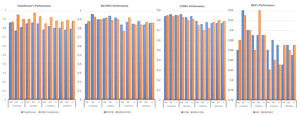
Figure 5: Classifiers performance with and without GRN.

TABLE IV: Transformer’s performance

Models	2.5% Data				5% Data				7.5% Data				10% Data
	Acc	Pre	Rec	F1	Acc	Pre	Rec	F1	Acc	Pre	Rec	F1	Acc	Pre	Rec	F1
Transformer	0.94	0.86	0.77	0.81	0.95	0.85	0.86	0.85	0.94	0.78	0.82	0.8	0.93	0.8	0.78	0.79
GRN-Transformer	0.96	0.87	0.95	0.9	0.98	0.9	0.97	0.93	0.96	0.85	0.92	0.88	0.96	0.87	0.89	0.88

TABLE V: BiLSTM’s Performance

Models	2.50% Data				5% Data				7.50% Data				10% Data
	Acc	Pre	Rec	F1	Acc	Pre	Rec	F1	Acc	Pre	Rec	F1	Acc	Pre	Rec	F1
BiLSTM	0.96	0.85	0.96	0.9	0.97	0.91	0.94	0.92	0.95	0.84	0.87	0.85	0.95	0.88	0.84	0.86
GRN-BiLSTM	0.96	0.88	0.93	0.9	0.97	0.92	0.89	0.9	0.95	0.77	0.92	0.84	0.95	0.84	0.87	0.86

TABLE VI: FCNN’s Performance

Models	2.5% Data				5% Data				7.5% Data				10% Data
	Acc	Pre	Rec	F1	Acc	Pre	Rec	F1	Acc	Pre	Rec	F1	Acc	Pre	Rec	F1
FCNN	0.95	0.84	0.86	0.85	0.95	0.86	0.83	0.84	0.93	0.79	0.76	0.78	0.92	0.77	0.77	0.77
GRN-FCNN	0.95	0.85	0.84	0.85	0.94	0.83	0.8	0.81	0.92	0.75	0.7	0.72	0.93	0.78	0.8	0.79

TABLE VII: MLP’s performance

Models	2.5% Data				5% Data				7.50% Data				10% Data
	Acc	Pre	Rec	F1	Acc	Pre	Rec	F1	Acc	Pre	Rec	F1	Acc	Pre	Rec	F1
MLP	0.96	0.86	0.94	0.9	0.96	0.89	0.89	0.89	0.96	0.86	0.88	0.87	0.95	0.83	0.87	0.85
GRN-MLP	0.96	0.88	0.93	0.9	0.96	0.86	0.94	0.89	0.95	0.82	0.84	0.83	0.95	0.87	0.86	0.87

TABLE VIII: Comparative of GRN-Transformer with semi-supervised label propagation (LP), and KNN

Models	2.5% Data				5% Data				7.5% Data				10% Data
	Acc	Pre	Rec	F1	Acc	Pre	Rec	F1	Acc	Pre	Rec	F1	Acc	Pre	Rec	F1
LP	0.96	0.87	0.93	0.9	0.97	0.89	0.93	0.91	0.95	0.81	0.91	0.86	0.94	0.78	0.86	0.82
KNN	0.96	0.87	0.92	0.89	0.97	0.89	0.95	0.92	0.95	0.78	0.93	0.85	0.95	0.8	0.91	0.85
GRN-Transformer	0.96	0.87	0.95	0.9	0.98	0.9	0.97	0.93	0.96	0.85	0.92	0.88	0.96	0.87	0.89	0.88

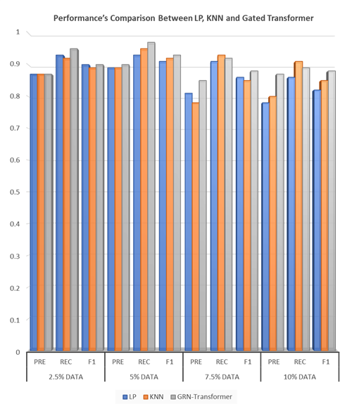
Figure 6: GRN-Transformer vs LP and KNN.

Table VIII and Fig. 6 compare the performance of three models, namely LP (semi-supervised label propagation), KNN (K-Nearest Neighbors), and GRN-Transformer, using different amounts of labeled data. When using 2.5% of the data for training, LP achieves an accuracy of 0.96, while both KNN and GRN-Transformer achieve the same accuracy. In terms of precision, LP, and KNN have a slightly higher value of 0.87 compared to GRN-Transformer’s 0.87. However, GRN-Transformer outperforms both LP and KNN regarding recall, achieving a value of 0.95 and also F1-score, with a value of 0.90. As the amount of labeled data increases to 5%, 7.5%, and 10%, the performance of all three models generally improves. GRN-Transformer consistently outperforms LP and KNN at each data point in accuracy, precision, recall, and F1-score. At 5% data, GRN-Transformer achieves the highest accuracy of 0.98, precision of 0.90, recall of 0.97, and F1-score of 0.93. LP and KNN follow closely behind with their corresponding scores. In conclusion, the table shows that the GRN-Transformer model demonstrates superior performance compared to both LP and KNN across all data percentages. It achieves higher accuracy, precision, recall, and F1 score, making it a promising model.

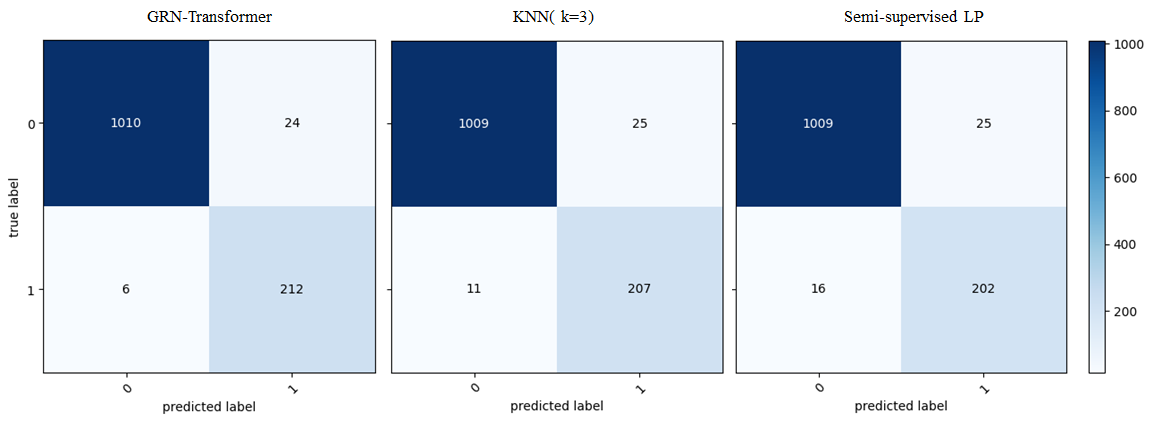
Figure 7: Confusion matrix between GRN-Transformer, KNN and LP.

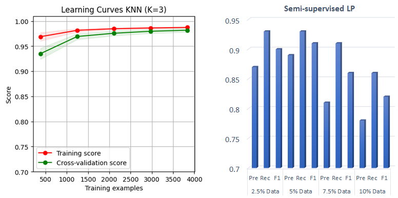
Figure 8: Limitation on KNN and LP’s performance varying on data portion.

The confusion matrix results for the GRN-Transformer, KNN, and LP algorithms were analyzed and summarized in Fig 7. The findings revealed that the GRN-Transformer demonstrated superior performance with only 30 cases of misclassification, a significantly smaller number compared to LP, which had 41 misclassified cases, and KNN, which had 36 misclassified cases. Remarkably, the misclassification rate of the GRN-Transformer was 26.8 percent lower than that of LP and 16.7 percent lower than KNN. These compelling results highlight the effectiveness and efficiency of the GRN-Transformer algorithm in handling the classification task, outperforming both LP and KNN methods.

Furthermore, the limitations of the KNN and LP algorithms are depicted in Fig. 8. Both algorithms face challenges regarding reaching their maximum performance and being heavily dependent on data availability. Specifically, the performance of the KNN (left) algorithm plateaus, with its score (both validation and training) remaining constant and showing no improvement despite an increase in data. On the other hand, the performance of the LP (right) algorithm demonstrates a strong dependence on the availability of labeled data, resulting in a downward trend in performance as the amount of labeled data increases. This observation confirms that LP struggles to provide stable predictions under varying data availability conditions. These insights shed light on the constraints and limitations associated with the KNN and LP algorithms, which should be considered in practical applications.

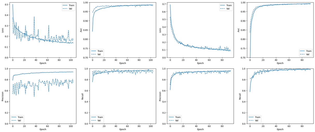
Figure 9: Learning curve performance based on the Transformer.

Theoretically, the superiority of Gated Linear Units (GLU) has been demonstrated and supported by findings in [38] and [56]. The remarkable success of GLU can be attributed to its ability to facilitate the learning of identity mappings, enabling the optimizer to transmit information more effectively through the network and, consequently, learn improved representations.

Experimentally, our experiment results confirm the above theoretical proof. Technically, the learning curve performance of Transformer models with and without GRN is illustrated in Fig. 9. The absence of GRN results in a highly fluctuating loss for the Transformer, making it challenging to identify minimum points in the loss space. Consequently, other evaluation criteria, such as precision, recall, and auc, also suffer from unstable and fluctuating performance. In contrast, the incorporation of GRN significantly enhances the Transformer’s performance. With GRN, the Transformer requires fewer epochs to converge to the minimal point, leading to a smoother loss curve during training and validation. This improvement in loss translates into remarkable enhancements in precision, recall, and AUC, culminating in outstanding performance for the GRN-Transformer. This insight highlights a crucial issue in training the Transformer, mainly when dealing with limited data availability—the complexity of the loss of space. Effectively addressing this challenge is vital to unlocking the Transformer’s full potential. GRN emerges as a powerful solution, helping the Transformer overcome the limitations of the loss of space and significantly improving its performance for various tasks, even with limited data availability. By leveraging GRN, the Transformer can achieve impressive results and outperform its counterparts in challenging scenarios.

V Limitations

The primary focus of the current study is the evaluation of PPG waveform quality through binary classification, differentiating between ”artifact” and ”normal” categories. However, this binary approach has limitations, as it fails to capture the finer nuances and subcategories of waveform quality. Future research should develop an improved methodology to classify waveform quality into more classes to address this limitation.

Furthermore, it is essential to clarify the scope of our analysis. Our investigation primarily compares the effectiveness of GRN and Transformer models as classifiers, specifically within supervised and semi-supervised learning paradigms. However, we have not explored unsupervised learning methods within this context. To address this gap, future investigations should consider incorporating unsupervised learning techniques, such as autoencoders, which have shown significant promise in related studies [57]. By including unsupervised learning, we can gain valuable insights into its efficacy compared to supervised and semi-supervised approaches, leading to a comprehensive understanding of the overall performance of diverse methods.

Additionally, it is essential to note that we have not analyzed the variant of GLU [56], which can potentially enhance the performance of the Transformer. Exploring and assessing the adaptability and effectiveness of these GLU variants could provide further improvements to the Transformer model.

In conclusion, future research efforts should address the current study’s limitations by adopting more approaches to signal quality classification, considering unsupervised learning techniques, and exploring the potential benefits of GLU variants for the Transformer model. Doing so can advance the understanding of PPG signal analysis and classification.

VI Conclusion

The study presents a comprehensive performance comparison of different ML classifiers, including MLP, FCNN, BiLSTM, and Transformer, both with and without the inclusion of Gate Residual Networks (GRNs), across various datasets with different percentages of training data. The study reveals that including GRNs significantly improves all classifiers’ performance, particularly enhancing the accuracy and overall performance of the Transformer model. The findings emphasize the effectiveness of GRNs in enhancing the learning capacity of ML classifiers in low-data scenarios.

Furthermore, the study also compares the performance of specific models with and without GRNs on different amounts of training data. The GRN-Transformer consistently outperforms the standard Transformer model in terms of accuracy, precision, recall, and F1-score across all data percentages, demonstrating the superiority of the GRN-Transformer for the classification task. Similarly, the GRN-BiLSTM model exhibits a competitive performance compared to the standard BiLSTM model, with slight improvements in precision and comparable recall scores. The performance comparison between FCNN and GRN-FCNN models shows that the choice depends on the specific evaluation metric and data percentage, with FCNN excelling in precision, while GRN-FCNN shows better recall values at lower data percentages. Moreover, the study compares semi-supervised learning LP, KNN, and GRN-Transformer models using different amounts of labeled data. GRN-Transformer consistently outperforms LP and KNN in accuracy, precision, recall, and F1-score.

In conclusion, the study highlights the importance of incorporating GRNs to enhance the performance of ML classifiers in low-data scenarios. The study provides valuable insights into choosing the most suitable models for specific applications based on the evaluation metrics and available data. Notably, to our best knowledge, the GRN-Transformer designed for artifact detection from PPG signals is the pioneering model of its kind. The results suggest that GRN-Transformer emerges as a promising model for the classification task, showcasing superior performance compared to other evaluated models.

Thanh-Dung Le (Member, IEEE) received a B.Eng. degree in mechatronics engineering from Can Tho University, Vietnam, an M.Eng. degree in electrical engineering from Jeju National University, S. Korea, and a Ph.D. in biomedical engineering from École de Technologie Supérieure (ETS), Canada. He is a postdoctoral fellow at the Biomedical Information Processing Laboratory, ETS. His research interests include applied machine learning approaches for biomedical informatics problems. Before that, he joined the Institut National de la Recherche Scientifique, Canada, where he researched classification theory and machine learning with healthcare applications. He received the merit doctoral scholarship from Le Fonds de Recherche du Quebec Nature et Technologies. He also received the NSERC-PERSWADE fellowship, Canada, and a graduate scholarship from the Korean National Research Foundation, S. Korea.

Clara Macabiau is a double degree student in Canada. After three years at the École nationale supérieure d’électrotechnique, d’électronique, d’informatique, d’hydraulique et des télécommunications (ENSEEIHT) engineering school in Toulouse, she is completing her master’s degree in electrical engineering at École de Technologie Supérieure (ETS), Canada. Her master’s project focuses on the detection of artifacts in photoplethysmography signals. She interests in signal processing, machine learning, and electronics.

Philippe Jouvet received the M.D. degree from Paris V University, Paris, France, in 1989, the M.D. specialty in pediatrics and the M.D. subspecialty in intensive care from Paris V University, in 1989 and 1990, respectively, and the Ph.D. degree in pathophysiology of human nutrition and metabolism from Paris VII University, Paris, in 2001. He joined the Pediatric Intensive Care Unit of Sainte Justine Hospital—University of Montreal, Montreal, QC, Canada, in 2004. He is currently the Deputy Director of the Research Center and the Scientific Director of the Health Technology Assessment Unit, Sainte Justine Hospital–University of Montreal. He has a salary award for research from the Quebec Public Research Agency (FRQS). He currently conducts a research program on computerized decision support systems for health providers. His research program is supported by several grants from the Sainte-Justine Hospital, Quebec Ministry of Health, the FRQS, the Canadian Institutes of Health Research (CIHR), and the Natural Sciences and Engineering Research Council (NSERC). He has published more than 160 articles in peer-reviewed journals. Dr. Jouvet gave more than 120 lectures in national and international congresses.

Rita Noumeir (Member, IEEE) received master’s and Ph.D. degrees in biomedical engineering from École Polytechnique of Montreal. She is currently a Full Professor with the Department of Electrical Engineering, École de Technologie Superieure (ETS), Montreal. Her main research interest is in applying artificial intelligence methods to create decision support systems. She has extensively worked in healthcare information technology and image processing. She has also provided consulting services in large-scale software architecture, healthcare interoperability, workflow analysis, and technology assessment for several international software and medical companies, including Canada Health Infoway.

References

- [1] B. B. Dean and et. al., “Use of electronic medical records for health outcomes research: a literature review,” Medical Care Research and Review, vol. 66, no. 6, pp. 611–638, 2009.
- [2] J. Latif and et. al., “Implementation and use of disease diagnosis systems for electronic medical records based on machine learning: A complete review,” IEEE Access, vol. 8, pp. 150 489–150 513, 2020.
- [3] M.-P. Matton and et. al., “Databases and computerized systems in picu: Electronic medical record in pediatric intensive care: Implementation process assessment,” J. Pediatr. Intensive Care, vol. 5, no. 3, 2016.
- [4] D. Brossier, R. El Taani, M. Sauthier, N. Roumeliotis, G. Emeriaud, and P. Jouvet, “Creating a high-frequency electronic database in the picu: the perpetual patient,” Pediatr. Crit. Care Med., vol. 19, no. 4, pp. e189–e198, 2018.
- [5] N. Roumeliotis, G. Parisien, S. Charette, E. Arpin, F. Brunet, and P. Jouvet, “Reorganizing care with the implementation of electronic medical records: a time-motion study in the picu,” Pediatr. Crit. Care Med., vol. 19, no. 4, pp. e172–e179, 2018.
- [6] A. Mathieu and et. al., “Validation process of a high-resolution database in a pediatric intensive care unit—describing the perpetual patient’s validation,” Journal of Evaluation in Clinical Practice, vol. 27, no. 2, pp. 316–324, 2021.
- [7] A. C. Dziorny and et. al., “Clinical decision support in the picu: Implications for design and evaluation,” Pediatr. Crit. Care Med., vol. 23, no. 8, pp. e392–e396, 2022.
- [8] T.-D. Le and et. al., “Detecting of a patient’s condition from clinical narratives using natural language representation,” IEEE Open J. Eng. Med. Biol., vol. 3, pp. 142–149, 2022.
- [9] M. Sauthier, G. Tuli, P. A. Jouvet, J. S. Brownstein, and A. G. Randolph, “Estimated pao2: A continuous and noninvasive method to estimate pao2 and oxygenation index,” Critical care explorations, vol. 3, no. 10, 2021.
- [10] G. Emeriaud, Y. M. López-Fernández, N. P. Iyer, M. M. Bembea, A. Agulnik, R. P. Barbaro, F. Baudin, A. Bhalla, W. B. De Carvalho, C. L. Carroll, et al., “Executive summary of the second international guidelines for the diagnosis and management of pediatric acute respiratory distress syndrome (palicc-2),” Pediatr. Crit. Care Med., vol. 24, no. 2, p. 143, 2023.
- [11] P. Jouvet and et. al., “A pilot prospective study on closed loop controlled ventilation and oxygenation in ventilated children during the weaning phase,” Critical Care, vol. 16, no. 3, pp. 1–9, 2012.
- [12] M. Wysocki, P. Jouvet, and S. Jaber, “Closed loop mechanical ventilation,” J. Clin. Monit. Comput., vol. 28, pp. 49–56, 2014.
- [13] B. L. Hill and et. al., “Imputation of the continuous arterial line blood pressure waveform from non-invasive measurements using deep learning,” Scientific reports, vol. 11, no. 1, p. 15755, 2021.
- [14] F. Fan and et. al., “Estimating spo 2 via time-efficient high-resolution harmonics analysis and maximum likelihood tracking,” IEEE J. Biomed. Health Inform., vol. 22, no. 4, pp. 1075–1086, 2017.
- [15] M. Clara and et al., “Label propagation techniques for artifact detection in imbalanced classes using photoplethysmograph signals,” Submitted to IEEE for possible publication, 2023.
- [16] H. W. Loh and et. al., “Application of photoplethysmography signals for healthcare systems: An in-depth review,” Computer Methods and Programs in Biomedicine, vol. 216, p. 106677, 2022.
- [17] D. Dao and et. al., “A robust motion artifact detection algorithm for accurate detection of heart rates from photoplethysmographic signals using time-frequency spectral features,” IEEE J. Biomed. Health Inform, vol. 21, no. 5, pp. 1242–1253, 2016.
- [18] P. Mehrgardt and et. al., “Deep learning fused wearable pressure and ppg data for accurate heart rate monitoring,” IEEE Sensors Journal, vol. 21, no. 23, pp. 27 106–27 115, 2021.
- [19] J. Liu and et. al., “Pca-based multi-wavelength photoplethysmography algorithm for cuffless blood pressure measurement on elderly subjects,” IEEE J. Biomed. Health Inform, vol. 25, no. 3, pp. 663–673, 2020.
- [20] D. A. Birrenkott and et. al., “A robust fusion model for estimating respiratory rate from photoplethysmography and electrocardiography,” IEEE Trans. Biomed. Eng., pp. 2033–2041, 2017.
- [21] B. Venema and et. al., “Robustness, specificity, and reliability of an in-ear pulse oximetric sensor in surgical patients,” IEEE J. Biomed. Health Inform, vol. 18, no. 4, pp. 1178–1185, 2013.
- [22] E. A. Alharbi and et. al., “Non-invasive solutions to identify distinctions between healthy and mild cognitive impairments participants,” IEEE J. Transl. Eng. Health Med., vol. 10, pp. 1–6, 2022.
- [23] C. Nwibor and et. al., “Remote health monitoring system for the estimation of blood pressure, heart rate, and blood oxygen saturation level,” IEEE Sensors Journal, vol. 23, no. 5, pp. 5401–5411, 2023.
- [24] S. Nabavi and et. al., “A robust fusion method for motion artifacts reduction in photoplethysmography signal,” IEEE Trans. Instrum. Meas., vol. 69, no. 12, pp. 9599–9608, 2020.
- [25] Z. Wang and et. al., “Time series classification from scratch with deep neural networks: A strong baseline,” in International joint conference on neural networks, 2017, pp. 1578–1585.
- [26] D. Marzorati and et. al., “Hybrid convolutional networks for end-to-end event detection in concurrent ppg and pcg signals affected by motion artifacts,” IEEE Trans. Biomed. Eng., vol. 69, no. 8, 2022.
- [27] S. Maqsood and et. al., “A benchmark study of machine learning for analysis of signal feature extraction techniques for blood pressure estimation using photoplethysmography (ppg),” Ieee Access, vol. 9, pp. 138 817–138 833, 2021.
- [28] T. Lin and et. al., “A survey of transformers,” AI Open, 2022.
- [29] Q. Li and et. al., “Dynamic time warping and machine learning for signal quality assessment of pulsatile signals,” Physiological measurement, vol. 33, no. 9, p. 1491, 2012.
- [30] Google, “Imbalanced data,” https://developers.google.com/machine-learning/data-prep/construct/sampling-splitting/imbalanced-data, 2023-06-09, online; accessed 2023-07-30.
- [31] J. Zurada, Introduction to ANN systems. West Publishing, 1992.
- [32] L. Noriega, “Multilayer perceptron tutorial,” School of Computing. Staffordshire University, vol. 4, no. 5, p. 444, 2005.
- [33] S. Albawi and et. al., “Understanding of a convolutional neural network,” in International Conference on Engineering and Technology, 2017.
- [34] M. Schuster and et. al., “Bidirectional recurrent neural networks,” IEEE Trans. Signal Process., vol. 45, no. 11, pp. 2673–2681, 1997.
- [35] A. Graves and et. al., “Framewise phoneme classification with bidirectional lstm and other neural network architectures,” Neural networks, vol. 18, no. 5-6, pp. 602–610, 2005.
- [36] A. Vaswani and et. al., “Attention is all you need,” Advances in neural information processing systems, vol. 30, 2017.
- [37] B. Lim, S. Ö. Arık, N. Loeff, and T. Pfister, “Temporal fusion transformers for interpretable multi-horizon time series forecasting,” International Journal of Forecasting, vol. 37, no. 4, pp. 1748–1764, 2021.
- [38] P. Savarese and D. Figueiredo, “Residual gates: A simple mechanism for improved network optimization,” in Int. Conf. Learn. Represent., 2017.
- [39] T.-D. Le and et. al., “A small-scale switch transformer and nlp-based model for clinical narratives classification,” arXiv preprint arXiv:2303.12892, 2023.
- [40] S. H. Lee and et. al., “Vision transformer for small-size datasets,” arXiv preprint arXiv:2112.13492, 2021.
- [41] R. Shao and X.-J. Bi, “Transformers meet small datasets,” IEEE Access, vol. 10, pp. 118 454–118 464, 2022.
- [42] M. Hahn, “Theoretical limitations of self-attention in neural sequence models,” Trans. Assoc. Comput. Linguist., vol. 8, pp. 156–171, 2020.
- [43] T. Sattler and et. al., “Understanding the limitations of cnn-based absolute camera pose regression,” in IEEE/CVF conference on computer vision and pattern recognition, 2019, pp. 3302–3312.
- [44] Y. N. Dauphin and et. al., “Language modeling with gated convolutional networks,” in International Conference on ML, 2017, pp. 933–941.
- [45] M. Liu and et. al., “Gated transformer networks for multivariate time series classification,” arXiv preprint arXiv:2103.14438, 2021.
- [46] F. Pedregosa and et. al, “Scikit-learn: Machine learning in Python,” Journal of Machine Learning Research, vol. 12, pp. 2825–2830, 2011.
- [47] F. Chollet and et. al., “keras,” 2015.
- [48] D. Hunter and et. al., “Selection of proper neural network sizes and architectures—a comparative study,” IEEE Transactions on Industrial Informatics, vol. 8, no. 2, pp. 228–240, 2012.
- [49] M. Popel and et. al., “Training tips for the transformer model,” arXiv preprint arXiv:1804.00247, 2018.
- [50] N. Srivastava and et. al., “Dropout: a simple way to prevent neural networks from overfitting,” The journal of machine learning research, vol. 15, no. 1, pp. 1929–1958, 2014.
- [51] X. Glorot and et. al., “Understanding the difficulty of training deep feedforward neural networks,” in Proceedings of the thirteenth international conference on artificial intelligence and statistics. JMLR Workshop and Conference Proceedings, 2010, pp. 249–256.
- [52] S. Ioffe and et. al., “Batch normalization: Accelerating deep network training by reducing internal covariate shift,” in International Conference on Machine Learning. PMLR, 2015, pp. 448–456.
- [53] N. Bjorck and et. al., “Understanding batch normalization,” Advances in Neural Information Processing Systems, vol. 31, 2018.
- [54] H. He and et. al., “Adasyn: Adaptive synthetic sampling approach for imbalanced learning,” in IEEE international joint conference on neural networks, 2008, pp. 1322–1328.
- [55] C. Goutte and et. al., “A probabilistic interpretation of precision, recall and f-score, with implication for evaluation,” in European conference on information retrieval. Springer, 2005, pp. 345–359.
- [56] N. Shazeer, “Glu variants improve transformer,” arXiv preprint arXiv:2002.05202, 2020.
- [57] J. Azar and et. al., “Deep recurrent neural network-based autoencoder for photoplethysmogram artifacts filtering,” Computers & Electrical Engineering, vol. 92, p. 107065, 2021.