Combining Proofs for Description Logic and Concrete Domain Reasoning (Technical Report)

Abstract

Logic-based approaches to AI have the advantage that their behavior can in principle be explained with the help of proofs of the computed consequences. For ontologies based on Description Logic (DL), we have put this advantage into practice by showing how proofs for consequences derived by DL reasoners can be computed and displayed in a user-friendly way. However, these methods are insufficient in applications where also numerical reasoning is relevant. The present paper considers proofs for DLs extended with concrete domains (CDs) based on the rational numbers, which leave reasoning tractable if integrated into the lightweight DL $\mathcal{E}\mathcal{L}_{\bot}$. Since no implemented DL reasoner supports these CDs, we first develop reasoning procedures for them, and show how they can be combined with reasoning approaches for pure DLs, both for $\mathcal{E}\mathcal{L}_{\bot}$ and the more expressive DL $\mathcal{ALC}$. These procedures are designed such that it is easy to extract proofs from them. We show how the extracted CD proofs can be combined with proofs on the DL side into integrated proofs that explain both the DL and the CD reasoning.

1 Introduction

Description Logics (DLs) [9] are a well-investigated family of logic-based knowledge representation languages, which are frequently used to formalize ontologies for various application domains. As the sizes of DL-based ontologies grow, tools that support improving the quality of such ontologies become more important. DL reasoners can be used to detect inconsistencies and to infer other implicit consequences, such as subsumption relationships. However, for developers or users of DL-based ontologies, it is often hard to understand why a consequence computed by the reasoner actually follows from the given, possibly very large ontology. In principle, such a consequence can be explained by producing a proof for it, which shows how the consequence can be derived from the axioms in the ontology by applying certain easy-to-understand inference rules. In recent work, we have investigated how proofs for consequences derived by DL reasoners can be computed [1, 2] and displayed [27] in a user-friendly way [4]. However, like previous work [17, 18], this was restricted to DLs without concrete domains.

Concrete domains [8, 24] (CDs) have been introduced to enable reference to concrete objects (such as numbers) and predefined predicates on these objects (such as numerical comparisons) when defining concepts. For example, assume that we measure the systolic and the diastolic blood pressure of patients. Then we can describe patients with a pulse pressure of 25 mmHg as $\textsf{{Patient}}\sqcap[\textsf{{sys}}-\textsf{{dia}}=25],$ where sys and dia are features that are interpreted as partial functions that return the systolic and the diastolic blood pressure of a patient, respectively, as rational numbers (if available). We can then state that such patients need attention using the general concept inclusion (GCI)

$$\textsf{{Patient}}\sqcap[\textsf{{sys}}-\textsf{{dia}}=25]\sqsubseteq\textsf{{NeedAttention}}.$$

In the presence of GCIs, integrating a CD into a DL may cause undecidability [25, 11] even if solvability of the constraint systems that can be formulated in the CD (in our example, sets of constraints of the form $x-y=q$ for $q\in\mathbb{Q}$) is decidable. One way to overcome this problem is to disallow role paths [16, 28, 7] in concrete domain restrictions, which means that these restrictions can only constrain feature values of single individuals, as in our example. Comparing feature values of different individuals, such as the age of a woman with that of her children, is then no longer possible.

For tractable (i.e., polynomially decidable) DLs like $\mathcal{E}\mathcal{L}_{\bot}$, preserving decidability is not sufficient: one wants to preserve tractability. As shown in [7], this is the case if one integrates a so-called p-admissible concrete domain into $\mathcal{E}\mathcal{L}_{\bot}$. The only numerical p-admissible concrete domain exhibited in [7] is the CD $\mathcal{D}_{\mathbb{Q},\textit{diff}}$, which supports constraints of the form $x=q$, $x>q$, and $x+q=y$ (for constants $q\in\mathbb{Q}$). Recently, additional p-admissible concrete domains have been introduced in [11], such as $\mathcal{D}_{\mathbb{Q},\textit{lin}}$, whose constraints are given by linear equations $\sum_{\_}{i=1}^{n}a_{\_}ix_{\_}i=b$. In the present paper, we will concentrate on these two p-admissible CDs, though the developed ideas and techniques can also be used for other CDs. The constraint used in our example can be expressed in both $\mathcal{D}_{\mathbb{Q},\textit{diff}}$ and $\mathcal{D}_{\mathbb{Q},\textit{lin}}$. Unfortunately, no implemented DL reasoner supports these two CDs. In particular, the highly efficient $\mathcal{E}\mathcal{L}_{\bot}$ reasoner Elk [19] does not support any concrete domain. Instead of modifying Elk or implementing our own reasoner for $\mathcal{E}\mathcal{L}_{\bot}$ with concrete domains, we develop here an iterative algorithm that interleaves Elk reasoning with concrete domain reasoning. For the CD reasoning, we could in principle employ existing algorithms and implementations, like Gaussian elimination or the simplex method [30, 15] for $\mathcal{D}_{\mathbb{Q},\textit{lin}}$, and SMT systems that can deal with difference logic [22, 6], such as Z3, for $\mathcal{D}_{\mathbb{Q},\textit{diff}}$. However, since our main purpose is to generate proofs, we develop our own reasoning procedures for $\mathcal{D}_{\mathbb{Q},\textit{diff}}$ and $\mathcal{D}_{\mathbb{Q},\textit{lin}}$, which may not be as efficient as existing ones, but can easily be adapted such that they produce proofs.

Proofs for reasoning results in $\mathcal{E}\mathcal{L}_{\bot}$ with a p-admissible CD can in principle be represented using the calculus introduced in [7] or an appropriate extension of the calculus employed by Elk. However, in these calculi, the result of CD reasoning (i.e., that a set of constraints is unsatisfiable or entails another constraint) is used as an applicability condition for certain rules, but the CD reasoning leading to the satisfaction of the conditions is not explained. Instead of augmenting such a proof with separate proofs on the CD side that show why the applicability conditions are satisfied, our goal is to produce a single proof that explains both the $\mathcal{E}\mathcal{L}_{\bot}$ and the CD reasoning in a uniform proof format.

We also consider the integration of the CDs $\mathcal{D}_{\mathbb{Q},\textit{diff}}$ and $\mathcal{D}_{\mathbb{Q},\textit{lin}}$ into the more expressive DL $\mathcal{ALC}$. To this purpose, we develop a new calculus for subsumption w.r.t. $\mathcal{ALC}$ ontologies, which is inspired by the one in [21], but has a better worst-case complexity, and then show how it can be extended to deal with concrete domain restrictions. We have implemented our reasoning and proof extraction approaches for DLs with concrete domains and have evaluated them on several self-created benchmarks designed specifically to challenge the CD reasoning and proof generation capabilities. More details about the experiments can be found in [3].

2 Description Logics with Concrete Domains

We recall the DLs $\mathcal{E}\mathcal{L}_{\bot}$ and $\mathcal{ALC}$ [9], and then discuss their extensions $\mathcal{E}\mathcal{L}_{\bot}[\mathcal{D}]$ and $\mathcal{ALC}[\mathcal{D}]$ with a concrete domain $\mathcal{D}$ [8, 7]. Following [11], we use square brackets to indicate that no role paths are allowed. We also introduce the two p-admissible concrete domains $\mathcal{D}_{\mathbb{Q},\textit{diff}}$ and $\mathcal{D}_{\mathbb{Q},\textit{lin}}$ [7, 11].

2.1 Description Logics

Starting with disjoint, countably infinite sets of concept and role names $\textsf{N}_{\textsf{C}}$ and $\textsf{N}_{\textsf{R}}$, $\mathcal{E}\mathcal{L}_{\bot}$ concepts are defined by the grammar $C,D::=\top\mid\bot\mid A\mid C\sqcap D\mid\exists r.C$, where $A\in\textsf{N}_{\textsf{C}}$ and $r\in\textsf{N}_{\textsf{R}}$. In $\mathcal{ALC}$, we additionally have negation $\lnot C$ as concept constructor. As usual, we then define $C\sqcup D:=\lnot(\lnot C\sqcap\lnot D)$ and $\forall r.C:=\lnot\exists r.\lnot C$. An $\mathcal{ALC}$ ($\mathcal{E}\mathcal{L}_{\bot}$) TBox (a.k.a. ontology) $\mathcal{O}$ is a finite set of general concept inclusions (GCIs, a.k.a. axioms) $C\sqsubseteq D$ for $\mathcal{ALC}$ ($\mathcal{E}\mathcal{L}_{\bot}$) concepts $C$ and $D$. We denote by $\mathsf{sub}(\mathcal{O})$ the set of subconcepts of all concepts appearing in $\mathcal{O}$.

An interpretation is a pair $\mathcal{I}=(\Delta^{\mathcal{I}},\cdot^{\mathcal{I}})$, where the domain $\Delta^{\mathcal{I}}$ is a non-empty set, and the interpretation function $\cdot^{\mathcal{I}}$ assigns to every concept name $A\in\textsf{N}_{\textsf{C}}$ a set $A^{\mathcal{I}}\subseteq\Delta^{\mathcal{I}}$ and to every role name $r\in\textsf{N}_{\textsf{R}}$ a binary relation $r^{\mathcal{I}}\subseteq\Delta^{\mathcal{I}}\times\Delta^{\mathcal{I}}$. This function is extended to complex concepts by defining $\top^{\mathcal{I}}:=\Delta^{\mathcal{I}}$, $\bot^{\mathcal{I}}:=\emptyset$, $(\exists r.C)^{\mathcal{I}}:=\{d\in\Delta^{\mathcal{I}}\mid\exists e\in\Delta^{\mathcal{I}}.\,(d,e)\in r^{\mathcal{I}}\land e\in C^{\mathcal{I}}\}$, $(\lnot C)^{\mathcal{I}}=\Delta^{\mathcal{I}}\setminus C^{\mathcal{I}}$, and $(C\sqcap D)^{\mathcal{I}}:=C^{\mathcal{I}}\cap D^{\mathcal{I}}$. The interpretation $\mathcal{I}$ is a model of $C\sqsubseteq D$ if $C^{\mathcal{I}}\subseteq D^{\mathcal{I}}$ (written $\mathcal{I}\models C\sqsubseteq D$), and it is a model of an ontology $\mathcal{O}$ ($\mathcal{I}\models\mathcal{O}$) if it is a model of all axioms in $\mathcal{O}$. An ontology $\mathcal{O}$ is consistent if it has a model, and an axiom $C\sqsubseteq D$ is entailed by $\mathcal{O}$ (written $\mathcal{O}\models C\sqsubseteq D$) if every model of $\mathcal{O}$ is a model of $C\sqsubseteq D$; in this case, we also say that $C$ is subsumed by $D$ w.r.t. $\mathcal{O}$. The classification of $\mathcal{O}$ is the set $\mathsf{CL}(\mathcal{O}):=\{\langle C,D\rangle\mid C,D\in\mathsf{sub}(\mathcal{O}),\ \mathcal{O}\models C\sqsubseteq D\}$. The three reasoning problems of deciding consistency, checking subsumption, and computing the classification are mutually reducible in polynomial time. Reasoning is P-complete in $\mathcal{E}\mathcal{L}_{\bot}$ and ExpTime-complete in $\mathcal{ALC}$ [9].

2.2 Concrete Domains.

Concrete domains have been introduced as a means to integrate reasoning about quantitative features of objects into DLs [8, 24, 11]. Given a set $\textsf{N}_{\textsf{P}}$ of concrete predicates and an arity $\textsf{ar}(P)\in\mathbb{N}$ for each $P\in\textsf{N}_{\textsf{P}}$, a concrete domain (CD) $\mathcal{D}=(\Delta^{\mathcal{D}},\cdot^{\mathcal{D}})$ over $\textsf{N}_{\textsf{P}}$ consists of a set $\Delta^{\mathcal{D}}$ and relations $P^{\mathcal{D}}\subseteq(\Delta^{\mathcal{D}})^{\textsf{ar}(P)}$ for all $P\in\textsf{N}_{\textsf{P}}$. We assume that $\textsf{N}_{\textsf{P}}$ always contains a nullary predicate $\bot$, interpreted as $\bot^{\mathcal{D}}:=\emptyset$, and a unary predicate $\top$ interpreted as $\top^{\mathcal{D}}:=\Delta^{\mathcal{D}}$. Given a set $\textsf{N}_{\textsf{V}}$ of variables, a constraint $P(x_{\_}1,\dots,x_{\_}{\textsf{ar}(P)})$, with $P\in\textsf{N}_{\textsf{P}}$ and $x_{\_}1,\dots,x_{\_}{\textsf{ar}(P)}\in\textsf{N}_{\textsf{V}}$, is a predicate whose argument positions are filled with variables.

Example 1.

The concrete domain $\mathcal{D}_{\mathbb{Q},\textit{diff}}$ has the set $\mathbb{Q}$ of rational numbers as domain and, in addition to $\top$ and $\bot$, the concrete predicates $x=q$, $x>q$, and $x+q=y$, for constants $q\in\mathbb{Q}$, with their natural semantics [7]. For example, $(x+q=y)^{\mathcal{D}_{\mathbb{Q},\textit{diff}}}=\{(p,r)\in\mathbb{Q}\times\mathbb{Q}\mid p+q=r\}$.

The concrete domain $\mathcal{D}_{\mathbb{Q},\textit{lin}}$ has the same domain as $\mathcal{D}_{\mathbb{Q},\textit{diff}}$, but its predicates other than $\{\top,\bot\}$ are given by linear equations $\sum_{\_}{i=1}^{n}a_{\_}ix_{\_}i=b$, for $a_{\_}i,b\in\mathbb{Q}$, with the natural semantics [11], e.g. the linear equation $x+y-z=0$ is interpreted as the ternary addition predicate $(x+y-z=0)^{\mathcal{D}_{\mathbb{Q},\textit{lin}}}=\{(p,q,s)\in\mathbb{Q}^{3}\mid p+q=s\}$.

The expressivity of these two CDs is orthogonal: The $\mathcal{D}_{\mathbb{Q},\textit{diff}}$ predicate $x>q$ cannot be expressed as a conjunction of constraints in $\mathcal{D}_{\mathbb{Q},\textit{lin}}$, whereas the $\mathcal{D}_{\mathbb{Q},\textit{lin}}$ predicate $x+y=0$ cannot be expressed in $\mathcal{D}_{\mathbb{Q},\textit{diff}}$. ∎

A constraint $\alpha=P(x_{\_}1,\dots,x_{\_}{\textsf{ar}(P)})$ is satisfied by an assignment $v\colon\textsf{N}_{\textsf{V}}\to\Delta^{\mathcal{D}}$ (written $v\models\alpha$) if $\big{(}v(x_{\_}1),\dots,v(x_{\_}{\textsf{ar}(P)})\big{)}\in P^{\mathcal{D}}$. An implication is of the form $\gamma\to\delta$, where $\gamma$ is a conjunction and $\delta$ a disjunction of constraints; it is valid if all assignments satisfying all constraints in $\gamma$ also satisfy some constraint in $\delta$ (written $\mathcal{D}\models\gamma\to\delta$). A conjunction $\gamma$ of constraints is satisfiable if $\gamma\to\bot$ is not valid. The CD $\mathcal{D}$ is convex if, for every valid implication $\gamma\to\delta$, there is a disjunct $\alpha$ in $\delta$ s.t. $\gamma\to\alpha$ is valid. It is p-admissible if it is convex and validity of implications is decidable in polynomial time. This condition has been introduced with the goal of obtaining tractable extensions of $\mathcal{E}\mathcal{L}_{\bot}$ with concrete domains [7].

Example 2.

The CDs $\mathcal{D}_{\mathbb{Q},\textit{diff}}$ and $\mathcal{D}_{\mathbb{Q},\textit{lin}}$ are both p-admissible, as shown in [7] and [11], respectively. However, if we combined their predicates into a single CD, then we would lose convexity. In fact, $\mathcal{D}_{\mathbb{Q},\textit{diff}}$ has the constraints $x>0$ and $x=0$. In addition, $y>0$ (of $\mathcal{D}_{\mathbb{Q},\textit{diff}}$) and $x+y=0$ (of $\mathcal{D}_{\mathbb{Q},\textit{lin}}$) express $x<0$. Thus, the implication $x+y=0\rightarrow x>0\vee x=0\vee y>0$ is valid, but none of the implications $x+y=0\rightarrow\alpha$ for $\alpha\in\{x>0,\ x=0,\ y>0\}$ is valid. ∎

To integrate a concrete domain $\mathcal{D}$ into description logics, the most general approach uses role paths $r_{\_}1\ldots r_{\_}k$ followed by a concrete feature $f$ to instantiate the variables in constraints, where the $r_{\_}i$ are roles and $f$ is interpreted as a partial function $f^{\mathcal{I}}\colon\Delta^{\mathcal{I}}\to\Delta^{\mathcal{D}}$. Using the concrete domain $\mathcal{D}_{\mathbb{Q},\textit{lin}}$, the concept $\textsf{{Human}}\sqcap\exists\textsf{{age}},\textsf{{parent}}\,\textsf{{age}}.[2x-y=0]$, for age being a concrete feature and parent a role name, describes humans with a parent that has twice their age. However, in the presence of role paths, p-admissibility of the CD does not guarantee decidability of the extended DL. Even if we just take the ternary addition predicate of $\mathcal{D}_{\mathbb{Q},\textit{lin}}$, the extension of $\mathcal{ALC}$ with it becomes undecidable [10], and the paper [11] exhibits a p-admissible CD whose integration into $\mathcal{E}\mathcal{L}_{\bot}$ destroys decidability. Therefore, in this paper we disallow role paths, which effectively restricts concrete domain constraints to the feature values of single abstract objects. Under this restriction, the integration of a p-admissible CD leaves reasoning in P for $\mathcal{E}\mathcal{L}_{\bot}$ [7] and in ExpTime for $\mathcal{ALC}$ [23]. Disallowing role paths also enables us to simplify the syntax by treating variables directly as concrete features.

Formally, the description logics $\mathcal{E}\mathcal{L}_{\bot}[\mathcal{D}]$ and $\mathcal{ALC}[\mathcal{D}]$ are obtained from $\mathcal{E}\mathcal{L}_{\bot}$ and $\mathcal{ALC}$ by allowing constraints $\alpha$ from the CD $\mathcal{D}$ to be used as concepts, where we employ the notation $[\alpha]$ to distinguish constraints visually from classical concepts. Interpretations $\mathcal{I}$ are extended by associating to each variable $x\in\textsf{N}_{\textsf{V}}$ a partial function $x^{\mathcal{I}}\colon\Delta^{\mathcal{I}}\to\Delta^{\mathcal{D}}$, and defining $[\alpha]^{\mathcal{I}}$ as the set of all $d\in\Delta^{\mathcal{I}}$ for which (a) the assignment $v^{\mathcal{I}}_{\_}d(x):=x^{\mathcal{I}}(d)$ is defined for all variables $x$ occurring in $\alpha$, and (b) $v^{\mathcal{I}}_{\_}d\models\alpha$.

Example 3.

Extending the medical example from the introduction, we can state that, for a patient in the intensive care unit, the heart rate and blood pressure are monitored, using the GCI $\textsf{{ICUpatient}}\sqsubseteq[\top(\textsf{{hr}})]\sqcap[\top(\textsf{{sys}})]\sqcap[\top(\textsf{{dia}})],$ which says that, for all elements of the concept ICUpatient, the values of the variables hr, sys, dia are defined. The pulse pressure pp can then be defined via $\textsf{{ICUpatient}}\sqsubseteq[\textsf{{sys}}-\textsf{{dia}}-\textsf{{pp}}=0].$ Similarly, the maximal heart rate can be defined by $\textsf{{ICUpatient}}\sqsubseteq[\textsf{{maxHR}}+\textsf{{age}}=220].$ All the constraints employed in these GCIs are available in $\mathcal{D}_{\mathbb{Q},\textit{lin}}$. One might now be tempted to use the GCI $\textsf{{ICUpatient}}\sqcap([\textsf{{pp}}>50]\sqcup[\textsf{{hr}}>\textsf{{maxHR}}])\sqsubseteq\textsf{{NeedAttention}}$ to say that ICU patients whose pulse pressure is larger than 50 mmHG or whose heart rate is larger than their maximal heart rate need attention. However, while $[\textsf{{pp}}>50]$ is a $\mathcal{D}_{\mathbb{Q},\textit{diff}}$ constraint, it is not available in $\mathcal{D}_{\mathbb{Q},\textit{lin}}$, and $[\textsf{{hr}}>\textsf{{maxHR}}]$ is available in neither. But we can raise an alert when the heart rate gets near the maximal one using $[\textsf{{maxHR}}-\textsf{{hr}}=5]\sqsubseteq\textsf{{NeedAttention}}$ since it is a statement over $\mathcal{D}_{\mathbb{Q},\textit{lin}}$. ∎

3 Combined Concrete and Abstract Reasoning

We start by showing how classification in $\mathcal{E}\mathcal{L}_{\bot}[\mathcal{D}]$ can be realized by interleaving a classifier for $\mathcal{E}\mathcal{L}_{\bot}$ with a constraint solver for $\mathcal{D}$. Then we describe our constraint solvers for $\mathcal{D}_{\mathbb{Q},\textit{lin}}$ and $\mathcal{D}_{\mathbb{Q},\textit{diff}}$.

3.1 Reasoning in $\mathcal{E}\mathcal{L}_{\bot}[\mathcal{D}]$

The idea is that we can reduce reasoning in $\mathcal{E}\mathcal{L}_{\bot}[\mathcal{D}]$ to reasoning in $\mathcal{E}\mathcal{L}_{\bot}$ by abstracting away CD constraints by new concept names, and then adding GCIs that capture the interactions between constraints. To be more precise, let $\mathcal{D}$ be a p-admissible concrete domain, $\mathcal{O}$ an $\mathcal{E}\mathcal{L}_{\bot}[\mathcal{D}]$ ontology, and $\mathcal{C}(\mathcal{O})$ the finite set of constraints occurring in $\mathcal{O}$. We consider the ontology $\mathcal{O}^{-\mathcal{D}}$ that results from replacing each $\alpha\in\mathcal{C}(\mathcal{O})$ by a fresh concept name $A_{\_}\alpha$. Since $\mathcal{D}$ is p-admissible, the valid implications over the constraints in $\mathcal{C}(\mathcal{O})$ can then be fully encoded by the $\mathcal{E}\mathcal{L}_{\bot}$ ontology

$$\mathcal{O}_{\_}\mathcal{D}\coloneqq{} \{A_{\_}{\alpha_{\_}1}\sqcap\dots\sqcap A_{\_}{\alpha_{\_}n}\sqsubseteq\bot\mid\alpha_{\_}1,\dots,\alpha_{\_}n\in\mathcal{C}(\mathcal{O}),\ \mathcal{D}\models\alpha_{\_}1\land\dots\land\alpha_{\_}n\to\bot\}\cup{}$$

$$\{A_{\_}{\alpha_{\_}1}\sqcap\dots\sqcap A_{\_}{\alpha_{\_}n}\sqsubseteq A_{\_}\beta\mid\alpha_{\_}1,\dots,\alpha_{\_}n,\beta\in\mathcal{C}(\mathcal{O}),\ \mathcal{D}\models\alpha_{\_}1\land\dots\land\alpha_{\_}n\to\beta\}.$$

The definition of $\mathcal{O}_{\_}\mathcal{D}$ is an adaptation of the construction introduced in [23, Theorem 2.14] for the more general case of admissible concrete domains. The problem is, however, that $\mathcal{O}_{\_}\mathcal{D}$ is usually of exponential size since it considers all subsets $\{\alpha_{\_}1,\dots,\alpha_{\_}n\}$ of $\mathcal{C}(\mathcal{O})$. Thus, the reasoning procedure for $\mathcal{E}\mathcal{L}_{\bot}[\mathcal{D}]$ obtained by using $\mathcal{O}^{-\mathcal{D}}\cup\mathcal{O}_{\_}\mathcal{D}$ as an abstraction of $\mathcal{O}$ would also be exponential. To avoid this blow-up, we test implications of the form $\alpha_{\_}1\land\dots\land\alpha_{\_}n\to\bot$ and $\alpha_{\_}1\land\dots\land\alpha_{\_}n\to\beta$ for validity in $\mathcal{D}$ only if this information is needed, i.e., if there is a concept $C$ that is subsumed by the concept names $A_{\_}{\alpha_{\_}1},\ldots,A_{\_}{\alpha_{\_}n}$.

The resulting approach for classifying the $\mathcal{E}\mathcal{L}_{\bot}[\mathcal{D}]$ ontology $\mathcal{O}$, i.e., for computing $\mathsf{CL}(\mathcal{O})=\{\langle C,D\rangle\mid C,D\in\mathsf{sub}(\mathcal{O}),\ \mathcal{O}\models C\sqsubseteq D\}$ is described in Algorithm 1, where we assume that $\mathsf{CL}(\mathcal{O}^{\prime})$ is computed by a polynomial-time $\mathcal{E}\mathcal{L}_{\bot}$ classifier, such as Elk, and that the validity of implications in $\mathcal{D}$ is tested using an appropriate constraint solver for $\mathcal{D}$. Since $\mathcal{D}$ is assumed to be p-admissible, there is a constraint solver that can perform the required tests in polynomial time. Thus, we can show that this algorithm is sound and complete, and also runs in polynomial time.

1 $\mathcal{O}^{\prime}:=\mathcal{O}^{-\mathcal{D}}$, $\mathcal{N}:=\emptyset$

2 while $\mathcal{N}\neq\mathsf{CL}(\mathcal{O}^{\prime})$ do

3       $\mathcal{N}:=\mathsf{CL}(\mathcal{O}^{\prime})$

4       foreach $C\in\mathsf{sub}(\mathcal{O}^{-\mathcal{D}})$ do

5             $\mathbf{D}_{\_}C:=\{\alpha\in\mathcal{C}(\mathcal{O})\mid\langle C,A_{\_}\alpha\rangle\in\mathsf{CL}(\mathcal{O}^{\prime})\}$

6             if $\mathcal{D}\models\bigwedge\mathbf{D}_{\_}C\rightarrow\bot$ then

7                  $\mathcal{O}^{\prime}:=\mathcal{O}^{\prime}\cup\big{\{}\bigsqcap_{\_}{\alpha\in\mathbf{D}_{\_}C}A_{\_}\alpha\sqsubseteq\bot\big{\}}$

8            else

9                  $\mathcal{O}^{\prime}:=\mathcal{O}^{\prime}\cup\big{\{}\bigsqcap_{\_}{\alpha\in\mathbf{D}_{\_}C}A_{\_}\alpha\sqsubseteq A_{\_}\beta\mid\beta\in\mathcal{C}(\mathcal{O}),\mathcal{D}\models\bigwedge\mathbf{D}_{\_}C\rightarrow\beta\big{\}}$

return $\mathcal{N}[A_{\_}\alpha\mapsto\alpha\mid\alpha\in\mathcal{C}(\mathcal{O})]$

Algorithm 1 Classification algorithm for $\mathcal{E}\mathcal{L}_{\bot}[\mathcal{D}]$

Theorem 1.

Algorithm 1 computes $\mathsf{CL}(\mathcal{O})$ in polynomial time.

Next, we show how constraint solvers for $\mathcal{D}_{\mathbb{Q},\textit{lin}}$ and $\mathcal{D}_{\mathbb{Q},\textit{diff}}$ can be obtained.

3.2 Reasoning in $\mathcal{D}_{\mathbb{Q},\textit{lin}}$

To decide whether a finite conjunction of linear equations is satisfiable or whether it implies another equation, we can use Gaussian elimination [30], which iteratively eliminates variables from a set of linear constraints in order to solve them. Each elimination step consists of a choice of constraint $\alpha$ that is used to eliminate a variable $x_{\_}i$ from another constraint $\gamma$ by adding a suitable multiple $q\in\mathbb{Q}$ of $\alpha$, such that, in the sum $\gamma+q\alpha$, the coefficient $a_{\_}i$ of $x_{\_}i$ becomes $0$. This can be used to eliminate $x_{\_}i$ from all constraints except $\alpha$, which can then be discarded to obtain a system of constraints with one less variable. For example, using $\alpha\colon 2x+3y=5$ to eliminate $x$ from $\gamma\colon 4x-6y=1$ using $q=-2$ yields the new equation $-12y=-9$.

To decide whether $\alpha_{\_}1\land\dots\land\alpha_{\_}n\to\bot$ is valid in $\mathcal{D}_{\mathbb{Q},\textit{lin}}$, we must test whether the system of linear equations $\alpha_{\_}1,\dots,\alpha_{\_}n$ is unsolvable. For this, we apply Gaussian elimination to this system. If we obtain a constraint of the form $0=b$ for non-zero $b$, then the system is unsolvable; otherwise, we obtain $0=0$ after all variables have been eliminated, which shows solvability. In case $\alpha_{\_}1\land\dots\land\alpha_{\_}n\to\bot$ is not valid, Algorithm 1 requires us to test whether $\alpha_{\_}1\land\dots\land\alpha_{\_}n\to\beta$ is valid for constraints $\beta$ different from $\bot$. This is the case iff the equation $\beta$ is a linear combination of the equations $\alpha_{\_}1,\dots,\alpha_{\_}n$. For this, we can also apply Gaussian elimination steps to eliminate all variables from $\beta$ using the equations $\alpha_{\_}1,\dots,\alpha_{\_}n$. If this results in the constraint $0=0$, it demonstrates that $\beta$ is a linear combination; otherwise, it is not.

In principle, one could use standard libraries from linear algebra (e.g. for Gaussian elimination or the simplex method [30, 15, 13]) to implement a constraint solver for $\mathcal{D}_{\mathbb{Q},\textit{lin}}$. We decided to create our own implementation based on Gaussian elimination, mainly for two reasons. First, most existing numerical libraries are optimized for performance and use floating-point arithmetic. Hence, the results may be erroneous due to repeated rounding [12]. Second, even if rational arithmetic with arbitrary precision is used [15], it is not trivial to extract from these tools a step-by-step account of how the verdict (valid or not) was obtained, which is a crucial requirement for extracting proofs.

3.3 Reasoning in $\mathcal{D}_{\mathbb{Q},\textit{diff}}$

The constraints of $\mathcal{D}_{\mathbb{Q},\textit{diff}}$ can in principle be simulated in difference logic, which consists of Boolean combinations of expressions of the form $x-y\leq q$, and for which reasoning can be done using the Bellman-Ford algorithm for detecting negative cycles [22, 6]. However, it is again not clear how proofs for the validity of implications can be extracted from the run of such a solver. For this reason, we implemented a simple saturation procedure that uses the rules in Fig. 1 to derive implied constraints, where side conditions are shown in gray; these rules are similar to the rewrite rules for DL-Lite queries with CDs in [5].

  $x=q$    $x=p$    $\mathsf{R_{\neq}}$ $\colon q\neq p$           $\bot$

  $x+q=y$    $y+p=z$    $\mathsf{R_{+}}$       $x+(q+p)=z$

     $x=x$    $\mathsf{R_{0}}$   $x+0=x$

  $x+q=y$    $x+p=y$    $\mathsf{R_{\neq}^{+}}$ $\colon q\neq p$                $\bot$

   $x=q$    $y=p$    $\mathsf{R_{-}}$   $x+(p-q)=y$

    $x+q=y$    $\mathsf{R_{\leftrightarrow}}$   $y+(-q)=x$

  $x=q$    $x>p$    $\mathsf{R_{<}}$ $\colon q<p$           $\bot$

  $x=q$    $x+p=y$    $\mathsf{R_{=}}$        $y=q+p$

  $x>q$    $x+p=y$    $\mathsf{R_{>}}$        $y>q+p$

Figure 1: Saturation rules for $\mathcal{D}_{\mathbb{Q},\textit{diff}}$ constraints

We eagerly apply the rules $\mathsf{R_{\neq}}$, $\mathsf{R_{<}}$, and $\mathsf{R_{\neq}^{+}}$, which means that we only need to keep one constraint of the form $x+q=y$ in memory, for each pair $(x,y)$. Since $x>q$ implies $x>p$ for all $p<q$, it similarly suffices to remember one unary constraint of the form $x=q$ or $x>q$ for each variable $x$. Apart from the three rules deriving $\bot$, we can prioritize rules in the order $\mathsf{R_{-}}$, $\mathsf{R_{\leftrightarrow}}$, $\mathsf{R_{0}}$, $\mathsf{R_{+}}$, $\mathsf{R_{=}}$, $\mathsf{R_{>}}$, since none of the later rules can enable the applications of earlier rules to derive new constraints. The full decision procedure is described in Algorithm 2.

Input: An implication $\bigwedge\mathbf{D}\to\beta$ in $\mathcal{D}_{\mathbb{Q},\textit{diff}}$

Output: $\mathsf{true}$ iff $\mathcal{D}_{\mathbb{Q},\textit{diff}}\models\bigwedge\mathbf{D}\to\beta$

1 $\mathbf{D}^{\prime}:=\mathsf{saturate}(\mathbf{D})$

2 if $\bot\in\mathbf{D}^{\prime}$ $\mathbf{or}$ $\beta\in\mathbf{D}^{\prime}$ then return $\mathsf{true}$

3 if $\beta$ is $x>q$ then

4       if $x=p\in\mathbf{D}^{\prime}$ with $p>q$ then return $\mathsf{true}$

5       if $x>p\in\mathbf{D}^{\prime}$ with $p\geq q$ then return $\mathsf{true}$

6      

return $\mathsf{false}$

Algorithm 2 Reasoning algorithm for $\mathcal{D}_{\mathbb{Q},\textit{diff}}$

Theorem 2.

Algorithm 2 terminates in time polynomial in the size of $\bigwedge\mathbf{D}\to\beta$ and returns $\mathsf{true}$ iff $\mathcal{D}_{\mathbb{Q},\textit{diff}}\models\bigwedge\mathbf{D}\to\beta$.

4 Proofs for $\mathcal{E}\mathcal{L}_{\bot}[\mathcal{D}]$ Entailments

Our goal is now to use the procedures described in Section 3 to obtain separate proofs for the DL part and the CD part of an entailment, which we then want to combine into a single proof, as illustrated in Fig. 2.

(a)   $C\sqsubseteq A_{\_}\alpha$     $C\sqsubseteq A_{\_}\beta$    $\mathsf{R}_{\_}\sqcap^{+}$       $C\sqsubseteq A_{\_}\alpha\sqcap A_{\_}\beta$        $A_{\_}\alpha\sqcap A_{\_}\beta\sqsubseteq A_{\_}\gamma\ (*)$        $\mathsf{R}_{\_}\sqsubseteq$                                  $C\sqsubseteq A_{\_}\gamma$ (b)   $2x+3y=5\vphantom{A_{\_}\beta}$            $4y=3\vphantom{A_{\_}\beta}$    $[-3]$   $-12y=-9\vphantom{A_{\_}\beta}$    $[2,1]$                $4x-6y=1\vphantom{A_{\_}\beta}$

$\Longrightarrow\qquad$ (c)   $C\sqsubseteq[2x+3y=5]$            $C\sqsubseteq[4y=3]$    $[-3]$   $C\sqsubseteq[-12y=-9]$    $[2,1]$                  $C\sqsubseteq[4x-6y=1]$ $\Longrightarrow\qquad$

Figure 2: (a) $\mathcal{E}\mathcal{L}_{\bot}$ proof over $\mathcal{O}^{\prime}$, (b) $\mathcal{D}_{\mathbb{Q},\textit{lin}}$ proof and (c) integrated $\mathcal{E}\mathcal{L}_{\bot}[\mathcal{D}_{\mathbb{Q},\textit{lin}}]$ proof.

Fig. 2(a) shows an example of an Elk-proof, a proof generated by the Elk reasoner [18] for the final ontology $\mathcal{O}^{\prime}\supseteq\mathcal{O}^{-\mathcal{D}}$ from Algorithm 1. The labels $\mathsf{R}_{\_}\sqsubseteq$ and $\mathsf{R}_{\_}\sqcap^{+}$ indicate the rules from the internal calculus of Elk [19], and $(*)$ marks an axiom added by Algorithm 1, where $\alpha$ is $2x+3y=5$, $\beta$ is $4y=3$, and $\gamma$ is $4x-6y=1$. We now describe how to obtain the proof (b) for the CD implication $\alpha\land\beta\to\gamma$, and how to integrate both proofs into the $\mathcal{E}\mathcal{L}_{\bot}[\mathcal{D}_{\mathbb{Q},\textit{lin}}]$ proof (c).

4.1 Proofs for the Concrete Domains

For $\mathcal{D}_{\mathbb{Q},\textit{diff}}$, the saturation rules in Fig. 1 can be seen as proof steps. Thus, the algorithms in [1, 2] can easily be adapted to extract $\mathcal{D}_{\mathbb{Q},\textit{diff}}$ proofs. Inferences due to Lines 2, 2 and 2 in Algorithm 2 are captured by the following additional rules:

  $$\bot \mathsf{R_{\bot}} \beta x=p \mathsf{R_{>}^{+}} \colon p>q x>q x>p \mathsf{R_{>}^{-}} \colon p\geq q x>q$$                                            

For $\mathcal{D}_{\mathbb{Q},\textit{lin}}$, inferences are Gaussian elimination steps that derive $\sigma+c\rho$ from linear constraints $\sigma$ and $\rho$, and we label them with $[1,c]$ to indicate that $\sigma$ is multiplied by $1$ and $\rho$ by $c$. This directly gives us a proof if the conclusion is $\bot$ (or, equivalently, $0=b$ for non-zero $b$). However, proofs for implications $\bigwedge\mathbf{D}\to\gamma$ need to be treated differently. The Gaussian method would use $\mathbf{D}$ to eliminate the variables from $\gamma$ to show that $\gamma$ is a linear combination of $\mathbf{D}$, and would yield a rather uninformative proof with final conclusion $0=0$. To obtain a proof with $\gamma$ as conclusion, we reverse the proof direction by recursively applying the following transformation starting from an inference step that has $\gamma$ as a premise:

$$\ignorespaces\ignorespaces\ignorespaces\ignorespaces\leavevmode\lower 23.15277pt\hbox{\vbox{\hbox{\hbox{\hskip 4.0pt\hbox{$\sigma$}\hskip 4.0pt}\hbox{\hskip 14.45377pt}\hbox{\hskip 4.0pt\hbox{$\rho$}\hskip 4.0pt}}\vskip-1.3pt\nointerlineskip\hbox{\hskip 0.0pt\lower-0.2pt\hbox{}\hbox to41.33804pt{\xleaders\hrule\hfill}\lower 1.55pt\hbox{\hskip 3.0pt\scriptsize$[1,c]$}}\vskip-1.3pt\nointerlineskip\hbox{\hskip 14.48326pt\hbox{\hbox{\hskip 4.0pt\hbox{$\tau$}\hskip 4.0pt}}}}}\ignorespaces\qquad\leadsto\qquad\ignorespaces\ignorespaces\ignorespaces\ignorespaces\leavevmode\lower 23.15277pt\hbox{\vbox{\hbox{\hbox{\hskip 4.0pt\hbox{$\rho$}\hskip 4.0pt}\hbox{\hskip 14.45377pt}\hbox{\hskip 4.0pt\hbox{$\tau$}\hskip 4.0pt}}\vskip-1.3pt\nointerlineskip\hbox{\hskip 0.0pt\lower-0.2pt\hbox{}\hbox to39.99545pt{\xleaders\hrule\hfill}\lower 1.55pt\hbox{\hskip 3.0pt\scriptsize$[-c,1]$}}\vskip-1.3pt\nointerlineskip\hbox{\hskip 13.14067pt\hbox{\hbox{\hskip 4.0pt\hbox{$\sigma$}\hskip 4.0pt}}}}}\ignorespaces \dagger$$ ()

Then we transform the next inference to obtain an inference that has $\tau$ as the conclusion, and continue this process until $0=0$ becomes a leaf, which we then remove from the proof.

In our example, we would start with the following “proof” for $\mathcal{D}\models\alpha\land\beta\to\gamma$:

  $$4x-6y=1 2x+3y=5 [1,-2] -12y=-9 4y=3 [1,3] 0=0$$                                                                                       

After applying two transformation steps ($\dagger$ ‣ 4.1), we obtain the proof in Fig. 2(b).

4.2 Combining the Proofs

It remains to integrate the concrete domain proofs into the DL proof over $\mathcal{O}^{-\mathcal{D}}$. As a consequence of Algorithm 1, in Fig. 2(a), the introduced concept names $A_{\_}\alpha$, $A_{\_}\beta$, $A_{\_}\gamma$ occur in axioms with the same left-hand side $C$. The idea is to add this DL context $C$ to every step of the CD proof (b) to obtain the $\mathcal{E}\mathcal{L}_{\bot}[\mathcal{D}]$-proof (c). This proof replaces the applications of $\mathsf{R}_{\_}\sqcap^{+}$ and $\mathsf{R}_{\_}\sqsubseteq$ in the original DL proof (a), and both (a) and (c) have essentially the same leafs and conclusion, except that the auxiliary concept names $A_{\_}\alpha,A_{\_}\beta,A_{\_}\gamma$ were replaced by the original constraints and the auxiliary axiom $(*)$ was eliminated. In general, such proofs can be obtained by simple post-processing of proofs obtained separately from the DL and CD reasoning components, and we conjecture that the integrated proof (c) is easier to understand in practice than the separate proofs (a) and (b), since the connection between the DL and CD contexts is shown in all steps.

Lemma 3.

Let $\mathcal{O}^{\prime}$ be the final ontology computed in Algorithm 1. Given an Elk-proof $\mathcal{P}^{\prime}$ for $\mathcal{O}^{\prime}\models C^{-\mathcal{D}}\sqsubseteq D^{-\mathcal{D}}$ and proofs for all $\mathcal{D}$-implications $\alpha_{\_}1\land\dots\land\alpha_{\_}n\to\beta$ used in $\mathcal{P}^{\prime}$, we can construct in polynomial time an $\mathcal{E}\mathcal{L}_{\bot}[\mathcal{D}]$-proof for $\mathcal{O}\models C\sqsubseteq D$.

5 Generating Proofs for $\mathcal{ALC}[\mathcal{D}]$

For $\mathcal{ALC}[\mathcal{D}]$, a black-box algorithm as for $\mathcal{E}\mathcal{L}_{\bot}[\mathcal{D}]$ is not feasible, even though we consider only p-admissible concrete domains and no role paths. The intuitive reason is that $\mathcal{ALC}$ itself is not convex, and we cannot simply use the classification result to determine which implications $\alpha_{\_}1\wedge\ldots\wedge\alpha_{\_}n\rightarrow\beta$ in $\mathcal{D}$ are relevant. On the other hand, adding all valid implications is not practical, as there can be exponentially many. We thus need a glass-box approach, i.e. a modified $\mathcal{ALC}$ reasoning procedure that determines the relevant CD implications on-demand.

Moreover, to obtain proofs for $\mathcal{ALC}[\mathcal{D}]$, we need a reasoning procedure that derives new axioms from old ones, and thus classical tableau methods [14, 26] are not suited. However, existing consequence-based classification methods for $\mathcal{ALC}$ [29] use complicated calculi that are not needed for our purposes. Instead, we use a modified version of a calculus from [21], which uses only three inference rules, but performs double exponentially many inferences in the worst case. Our modification ensures that we perform at most exponentially many inferences, and are thus worst-case optimal for the ExpTime-complete $\mathcal{ALC}[\mathcal{D}]$.

5.1 A Simple Resolution Calculus for $\mathcal{ALC}$

The calculus represents GCIs $\top\sqsubseteq L_{\_}1\sqcup\dots\sqcup L_{\_}n$ as clauses of the form

$$L_{\_}1\sqcup\ldots\sqcup L_{\_}n\qquad L_{\_}i\ ::=\ A\ \mid\ \neg A\ \mid\ \exists r.D\ \mid\ \forall r.D$$

where $n\geq 0$, $A,D\in\textsf{N}_{\textsf{C}}$ and $r\in\textsf{N}_{\textsf{R}}$. To decide $\mathcal{O}\models A\sqsubseteq B$, we normalize $\mathcal{O}$ into a set of clauses, introducing fresh concept names for concepts under role restrictions, and add two special clauses $A_{\_}\text{LHS}\sqcup A$, $A_{\_}\text{RHS}\sqcup\neg B$, with fresh concept names $A_{\_}\text{LHS}$ and $A_{\_}\text{RHS}$. The latter are used to track relevant inferences for constructing the final proof, for which we transform all clauses back into GCIs.

A1: $\dfrac{C_{\_}1\sqcup A,\quad C_{\_}2\sqcup\neg A}{C_{\_}1\sqcup C_{\_}2}$

r1: $\dfrac{C\sqcup\exists r.D,\quad C_{\_}1\sqcup\forall r.D_{\_}1,\ \ldots,\ C_{\_}n\sqcup\forall r.D_{\_}n,\quad\neg D_{\_}1\sqcup\ldots\sqcup\neg D_{\_}n}{C\sqcup C_{\_}1\sqcup\ldots\sqcup C_{\_}n}$

r2: $\dfrac{C\sqcup\exists r.D,\quad C_{\_}1\sqcup\forall r.D_{\_}1,\ \ldots,\ C_{\_}n\sqcup\forall r.D_{\_}n,\quad\neg D\sqcup\neg D_{\_}1\sqcup\ldots\sqcup\neg D_{\_}n}{C\sqcup C_{\_}1\sqcup\ldots\sqcup C_{\_}n}$

Figure 3: Inference rules for $\mathcal{ALC}$ clauses.

Our inference rules are shown in Fig. 3. A1 is the standard resolution rule from first-order logic, which is responsible for direct inferences on concept names. The rules r1 and r2 perform inferences on role restrictions. They consider an existential role restriction $\exists r.D$ and a (possibly empty) set of value restrictions over $r$, whose conjunction is unsatisfiable due to a clause over the nested concepts. The concept $D$ may not be relevant for this, which is why there are two rules. Those rules are the main difference to the original calculus in [21], where a more expensive, incremental mechanism was used instead. To transform this calculus into a practical method, we use optimizations common for resolution-based reasoning in first-order logic: ordered resolution, a set-of-support strategy, as well as backward and forward subsumption deletion. In particular, our set-of-support strategy starts with a set of support clauses containing only the clauses with $A_{\_}\text{LHS}$ and $A_{\_}\text{RHS}$. Inferences are always performed with at least one clause from this set, and the conclusion becomes a new support clause. If a support clause contains a literal $\exists r.D$/$\forall r.D$, we also add all clauses containing $\neg D$ as support clauses [20].

5.2 Incorporating the Concrete Domain and Creating the Proof

To incorporate concrete domains, we again work on the translation $\mathcal{O}^{-\mathcal{D}}$ replacing each constraint $\alpha$ with $A_{\_}\alpha$. In $\mathcal{ALC}[\mathcal{D}]$, constraints can also occur in negated form, which means that we can have literals $\neg A_{\_}\alpha$ expressing the negation of a constraint. We keep track of the set D of concrete domain constraints $\alpha$ for which $A_{\_}\alpha$ occurs positively in a support clause. We then use the proof procedure for $\mathcal{D}$ (see Section 4.1) to generate all implications of the form $\alpha_{\_}1\wedge\ldots\wedge\alpha_{\_}n\rightarrow\beta$, where $\{\alpha_{\_}1$, $\ldots$, $\alpha_{\_}n\}\subseteq\mathbf{D}$ is subset-minimal, for which we add the corresponding clauses $\neg A_{\_}{\alpha_{\_}1}\sqcup\ldots\sqcup\neg A_{\_}{\alpha_{\_}n}\sqcup A_{\_}\beta$. If $\beta=\bot$, we instead add $\neg A_{\_}{\alpha_{\_}1}\sqcup\ldots\sqcup\neg A_{\_}{\alpha_{\_}n}$.

Theorem 4.

Let $\mathcal{O}$ be an $\mathcal{ALC}[\mathcal{D}]$ ontology and $\mathcal{N}$ the normalization of $\mathcal{O}^{-\mathcal{D}}$. Then our method takes at most exponential time, and it derives $A_{\_}\text{LHS}\sqcup A_{\_}\text{RHS}$ or a subclause from $\mathcal{N}$ iff $\mathcal{O}\models C\sqsubseteq D$.

Proofs generated using the calculus operate on the level of clauses. We transform them into proofs of $\mathcal{O}^{-\mathcal{D}}\models A\sqsubseteq B$ by 1) adding inference steps that reflect the normalization, 2) if necessary, adding an inference to produce $A_{\_}\text{LHS}\sqcup A_{\_}\text{RHS}$ from a subclause 3) replacing $A_{\_}\text{LHS}$ by $\neg A$ and $A_{\_}\text{RHS}$ by $B$, 4) replacing all other introduced concept names by the complex concepts they were introduced for, and 5) transforming clauses into more human-readable GCIs using some simple rewriting rules (see the appendix for details). In the resulting proof, the initial clauses $A\sqcup A_{\_}{LHS}$ and $\neg B\sqcup A_{\_}{RHS}$ then correspond to the tautologies $A\sqsubseteq A$ and $B\sqsubseteq B$. To get a proof for $\mathcal{O}\models A\sqsubseteq B$, we use a procedure similar to the one from Section 4.2 to integrate concrete domain proofs. Because the integration requires only simple structural transformations, the complexity of computing the combined proofs is determined by the corresponding complexities for the DL and the concrete domain. We can thus extend the approaches from [1, 2] to obtain complexity bounds for finding proofs of small size and depth.

Theorem 5.

For $\mathcal{D}\in\{\mathcal{D}_{\mathbb{Q},\textit{lin}},\mathcal{D}_{\mathbb{Q},\textit{diff}}\}$, deciding the existence of a proof of at most a given size can be done in NP for $\mathcal{E}\mathcal{L}_{\bot}[\mathcal{D}]$, and in NExpTime for $\mathcal{ALC}[\mathcal{D}]$. For proof depth, the corresponding problem is in P for $\mathcal{E}\mathcal{L}_{\bot}[\mathcal{D}_{\mathbb{Q},\textit{diff}}]$, in NP for $\mathcal{E}\mathcal{L}_{\bot}[\mathcal{D}_{\mathbb{Q},\textit{lin}}]$, and in ExpTime for $\mathcal{ALC}[\mathcal{D}]$ (for both concrete domains).

6 Implementation and Experiments

We implemented the algorithms described above and evaluated their performance and the produced proofs on the self-created benchmarks Diet, Artificial, D-Sbj and D-Obj, each of which consists of multiple instances scaling from small to medium-sized ontologies. The latter two benchmarks are formulated in $\mathcal{E}\mathcal{L}_{\bot}[\mathcal{D}_{\mathbb{Q},\textit{diff}}]$, the rest in $\mathcal{E}\mathcal{L}_{\bot}[\mathcal{D}_{\mathbb{Q},\textit{lin}}]$. Our tool is written using Java 8 and Scala. We used Elk 0.5, Lethe 0.85 and OWL API 4. The experiments were performed on Debian Linux 10 (24 Intel Xeon E5-2640 CPUs, 2.50GHz) with 25 GB maximum heap size and a timeout of 3 minutes for each task. Fig. 5 shows the runtimes of the approaches for $\mathcal{E}\mathcal{L}_{\bot}[\mathcal{D}]$ from Sections 3 and 4 for reasoning and explanation depending on the problem size, which counts all occurrences of concept names, role names, and features in the ontology. A more detailed description of the benchmarks and results can be found in the appendix.

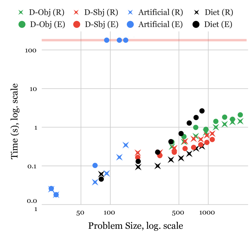
Figure 4: $\mathcal{E}\mathcal{L}_{\bot}[\mathcal{D}]$: time for reasoning (R) and explanation (E) vs. problem size

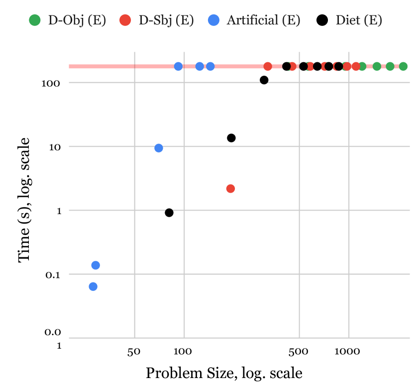
Figure 5: $\mathcal{ALC}[\mathcal{D}]$: total reasoning and explanation time vs. problem size

We observe that pure reasoning time (crosses in Fig. 5) scales well w.r.t. problem size. Producing proofs was generally more costly than reasoning, but the times were mostly reasonable. However, there are several Artificial instances for which the proof construction times out (blue dots). This is due to the nondeterministic choices of which linear constraints to use to eliminate the next variable, which we resolve using the Dijkstra-like algorithm described in [2], which results in an exponential runtime in the worst case. Another downside is that some proofs were very large ($>2000$ inference steps in D-Obj). However, we designed our benchmarks specifically to challenge the CD reasoning and proof generation capabilities (in particular, nearly all constraints in each ontology are necessary to entail the target axiom), and these results may improve for realistic ontologies.

Further analysis revealed that the reasoning times were often largely due to the calls to Elk (ranging from $23\%$ in Diet to $75\%$ in Artificial), which shows that the CD reasoning does not add a huge overhead, unless the number of variables per constraint grows very large (e.g. up to $88$ in Diet). In comparison to the incremental use of Elk as a black-box reasoner, the hypothetical “ideal” case of calling Elk only once on the final saturated ontology $\mathcal{O}^{\prime}$ would not save a lot of time (average gain ranging from $42\%$ in Diet to $14\%$ in D-Obj), which shows that the incremental nature of our approach is also not a bottleneck.

Fig. 5 shows the runtime of the $\mathcal{ALC}[\mathcal{D}]$ calculus from Section 5. As expected, it performs worse than the dedicated $\mathcal{E}\mathcal{L}_{\bot}[\mathcal{D}]$ algorithms. In particular, currently there is a bottleneck for the $\mathcal{D}_{\mathbb{Q},\textit{diff}}$ benchmarks (D-Sbj and D-Obj) that is due an inefficiency in the computation of the relevant CD implications $\alpha_{\_}1\land\dots\land\alpha_{\_}n\to\beta$. In order to evaluate the increased expressivity supported by the $\mathcal{ALC}[\mathcal{D}]$ reasoner, we have also incorporated axioms with negation and universal restrictions into the Artificial benchmark. Currently, however, the reasoner can solve only the smallest such instance before reaching the timeout.

We also compared our CD reasoning algorithms with Z3 [13], which supports linear arithmetic (for $\mathcal{D}_{\mathbb{Q},\textit{lin}}$) and difference logic (for $\mathcal{D}_{\mathbb{Q},\textit{diff}}$). Ignoring the overhead stemming from the interface between Java and C++, the runtime of both approaches was generally in the same range, but our algorithms were faster on many CD reasoning problems. This may be due to the fact that, although our algorithms for $\mathcal{D}_{\mathbb{Q},\textit{lin}}$ and $\mathcal{D}_{\mathbb{Q},\textit{diff}}$ are not optimized very much, they are nevertheless tailored towards very specific convex fragments: linear arithmetic with only $=$, and difference logic with only $x+q=y$ and $x>q$, respectively.

7 Conclusion

We have shown that it is feasible to support p-admissible concrete domains in DL reasoning algorithms, and even to produce integrated proofs for explaining consequences in the DLs $\mathcal{E}\mathcal{L}_{\bot}[\mathcal{D}]$ and $\mathcal{ALC}[\mathcal{D}]$, for the p-admissible concrete domains $\mathcal{D}_{\mathbb{Q},\textit{lin}}$ and $\mathcal{D}_{\mathbb{Q},\textit{diff}}$. In this work, we have restricted our attention to ontologies containing only GCIs (i.e., TBoxes) and to classification as the main reasoning problem. However, the extension of our methods to data and reasoning about individuals, e.g. $\textsf{{fred}}:\textsf{{ICUpatient}}\sqcap[\textsf{{hr}}=90]$, encoded in so-called ABoxes [9], is straightforward. Likewise, the approach for computing $\mathcal{E}\mathcal{L}_{\bot}[\mathcal{D}]$ proofs can be generalized to use other reasoning calculi for $\mathcal{E}\mathcal{L}_{\bot}$ instead of the one employed by Elk, which makes very small proof steps and thus generates rather large proofs.

One major problem with using proofs to explain consequences is that they may become quite large. This problem already occurs for pure DLs without CDs, and has also shown up in some of our benchmarks in this paper. One possibility to alleviate this problem is to use an interactive proof visualization tool like Evonne [27], which allows zooming into parts of the proof and hiding uninteresting or already inspected parts. Since the integrated proofs that we generate have the same shape as pure DL proofs, they can be displayed using Evonne. It would, however, be interesting to add features tailored to CD reasoning, such as visualizing the solution space of a system of linear equations.

In Example 3, we have seen that it would be useful to have the constraints of $\mathcal{D}_{\mathbb{Q},\textit{lin}}$ and $\mathcal{D}_{\mathbb{Q},\textit{diff}}$ available in a single CD. Such a CD $\mathcal{D}$ would still preserve decidability if integrated into $\mathcal{ALC}$. However, since $\mathcal{D}$ is no longer convex, our reasoning approach for $\mathcal{ALC}[\mathcal{D}]$ does not apply. Thus, it would also be interesting to see whether this approach can be extended to admissible CDs $\mathcal{D}$ [8, 23], i.e. CDs that are closed under negation and for which satisfiability of sets of constraints is decidable.

Acknowledgments

This work was supported by the DFG grant 389792660 as part of TRR 248 (https://perspicuous-computing.science).

Appendix A Omitted Proofs in Sections 3 and 4

See 1

Proof.

We first observe that, in each iteration, the while loop adds at most polynomially many axioms to $\mathcal{O}^{\prime}$ (at most one for each concept $C\in\mathsf{sub}(\mathcal{O}^{-\mathcal{D}})$ and constraint $\beta\in\mathcal{C}(\mathcal{O})$), which are of polynomial size. Therefore, $\mathsf{CL}(\mathcal{O}^{\prime})$ can always be computed in polynomial time [7] in Lines 1 and 1. Moreover, there are at most polynomially many iterations since we only add axioms to $\mathcal{O}^{\prime}$, and thus due to the monotonicity of entailment, each set $\mathbf{D}_{\_}C$ in Line 1 monotonically increases from one iteration to the next, and is bounded by $\mathcal{C}(\mathcal{O})$. Since the loop terminates once all sets $\mathbf{D}_{\_}C$ remain the same, there can be at most $\lvert\mathsf{sub}(\mathcal{O}^{-\mathcal{D}})\rvert\cdot\lvert\mathcal{C}(\mathcal{O})\rvert$ iterations of the while loop.

It remains to prove correctness. In each step, $\mathcal{O}^{\prime}[A_{\_}\alpha\mapsto\alpha\mid\alpha\in\mathcal{C}(\mathcal{O})]$ contains only axioms that are entailed by $\mathcal{O}$, since the concept names $A_{\_}\alpha$ replace exactly the occurrences of the concrete constraints $\alpha$ occurring in $\mathcal{O}$. Consequently, if the output of the algorithm contains $\langle C,D\rangle$, then $\mathcal{O}\models C\sqsubseteq D$, which means that the algorithm is sound. It remains to show completeness, i.e. that the output contains all such tuples. Take two concepts $C^{\dagger},D^{\dagger}\in\mathsf{sub}(\mathcal{O})$ such that $\langle C^{\dagger},D^{\dagger}\rangle$ is not returned. We construct a model $\mathcal{I}$ of $\mathcal{O}$, based on the contents of $\mathcal{O}^{\prime}$ and $\mathcal{N}=\mathsf{CL}(\mathcal{O}^{\prime})$ in the last iteration, such that $\mathcal{I}\not\models C^{\dagger}\sqsubseteq D^{\dagger}$. We start with a model $\mathcal{I}^{\prime}$ of the final ontology $\mathcal{O}^{\prime}$:

• $\Delta^{\mathcal{I}^{\prime}}:=\{C\in\mathsf{sub}(\mathcal{O}^{-\mathcal{D}})\mid\langle C,\bot\rangle\not\in\mathcal{N}\}$,

• for all $A\in\textsf{N}_{\textsf{C}}$, $A^{\mathcal{I}^{\prime}}:=\{C\in\Delta^{\mathcal{I}^{\prime}}\mid\langle C,A\rangle\in\mathcal{N}\}$,

• for all $r\in\textsf{N}_{\textsf{R}}$, $r^{\mathcal{I}^{\prime}}:=\{\langle C,D\rangle\in\Delta^{\mathcal{I}^{\prime}}\times\Delta^{\mathcal{I}^{\prime}}\mid\langle C,\exists r.D\rangle\in\mathcal{N}\}$

Since $\mathsf{CL}(\mathcal{O}^{\prime})$ computes all entailed inclusions between subconcepts in $\mathcal{O}^{\prime}$, one can easily show that $\mathcal{I}^{\prime}\models\mathcal{O}^{\prime}$ [19]: from the construction it follows by induction on the structure of $C,D\in\mathsf{sub}(\mathcal{O}^{-\mathcal{D}})$ that $C\in D^{\mathcal{I}^{\prime}}$ iff $\langle C,D\rangle\in\mathcal{N}$ and $\langle C,\bot\rangle\not\in\mathcal{N}$. Let $C\sqsubseteq D\in\mathcal{O}^{\prime}$ and $E\in C^{\mathcal{I}^{\prime}}$. Then, $\langle E,C\rangle\in\mathcal{N}$, and since $\mathcal{O}^{\prime}\models C\sqsubseteq D$, also $\langle E,D\rangle\in\mathcal{N}$, and thus $E\in D^{\mathcal{I}^{\prime}}$.

We argue that $\mathcal{I}^{\prime}$ can be extended to an interpretation $\mathcal{I}$ such that, for each $\alpha\in\mathcal{C}(\mathcal{O})$, we have $A_{\_}\alpha^{\mathcal{I}^{\prime}}=\alpha^{\mathcal{I}}$. It is possible to ensure $A_{\_}\alpha^{\mathcal{I}^{\prime}}\subseteq\alpha^{\mathcal{I}}$, because, if $\mathbf{D}_{\_}C$ for some domain element $C\in\Delta^{\mathcal{I}^{\prime}}$ is unsatisfiable, we would have added an axiom $\bigsqcap_{\_}{\alpha\in\mathbf{D}_{\_}C}A_{\_}\alpha\sqsubseteq\bot$ in Line 1, and by completeness of $\mathsf{CL}(\mathcal{O}^{\prime})$, we would have added $\langle C,\bot\rangle$ to $\mathcal{N}$, and thus not included $C$ in $\Delta^{\mathcal{I}^{\prime}}$. Consequently, we can assign values to the concrete features such that all constraints in $\mathbf{D}_{\_}C$ are satisfied, i.e. $C\in A_{\_}\alpha^{\mathcal{I}^{\prime}}$ implies $C\in\alpha^{\mathcal{I}}$, since $A_{\_}\alpha\in\mathbf{D}_{\_}C$ by construction. However, we have to ensure that for all $\alpha\in\mathcal{C}(\mathcal{O})$, also $\alpha^{\mathcal{I}}\subseteq A_{\_}\alpha^{\mathcal{I}^{\prime}}$ holds, because otherwise there might be GCIs in $\mathcal{O}$ with concrete constraints on the left-hand side that are not satisfied. Intuitively, we have to make sure that we do not accidentally satisfy more concrete domain constraints than necessary. For a fixed $C$, let $\overline{\mathbf{D}}_{\_}C:=\{\beta\in\mathcal{C}(\mathcal{O})\mid\langle C,A_{\_}\beta\rangle\not\in\mathcal{N}\}$. Due to Line 1, there is no $\beta\in\overline{\mathbf{D}}_{\_}C$ such that $\mathcal{D}\models\bigwedge\mathbf{D}_{\_}C\rightarrow\beta$. By convexity of $\mathcal{D}$, this implies $\mathcal{D}\not\models\bigwedge\mathbf{D}_{\_}C\rightarrow\bigvee\overline{\mathbf{D}}_{\_}C$. In other words, we can find an assignment to the concrete features $x^{\mathcal{I}}(C)$ such that every constraint in $\mathbf{D}_{\_}C$ is satisfied, and no constraint in $\overline{\mathbf{D}}_{\_}C$ is satisfied. Doing this for all domain elements $C\in\Delta^{\mathcal{I}^{\prime}}$, we ensure that $A_{\_}\alpha^{\mathcal{I}^{\prime}}=\alpha^{\mathcal{I}}$ for all $\alpha\in\mathcal{C}(\mathcal{O})$, and thus $\mathcal{I}\models\mathcal{O}$.

We now show that $\mathcal{I}\not\models C^{\dagger}\sqsubseteq D^{\dagger}$ by proving that $C^{\prime}\in(C^{\prime})^{\mathcal{I}}=(C^{\dagger})^{\mathcal{I}}$ and $C^{\prime}\notin(D^{\prime})^{\mathcal{I}}=(D^{\dagger})^{\mathcal{I}}$, where $C^{\prime}$ and $D^{\prime}$ result from replacing in $C^{\dagger}$ and $D^{\dagger}$ each $\alpha\in\mathcal{C}(\mathcal{O})$ by $A_{\_}\alpha$. From our assumption that $\langle C^{\dagger},D^{\dagger}\rangle$ is not returned by Algorithm 1, we know that $\langle C^{\prime},D^{\prime}\rangle\notin\mathcal{N}$. Therefore, by completeness of $\mathsf{CL}(\mathcal{O}^{\prime})=\mathcal{N}$, we cannot have $\langle C^{\prime},\bot\rangle\in\mathcal{N}$, and thus $C^{\prime}\in\Delta^{\mathcal{I}^{\prime}}$ and $C^{\prime}\notin(D^{\prime})^{\mathcal{I}^{\prime}}=(D^{\prime})^{\mathcal{I}}$. Completeness of $\mathsf{CL}(\mathcal{O}^{\prime})$ also yields that $\langle C^{\prime},C^{\prime}\rangle\in\mathcal{N}$, and thus $C^{\prime}\in(C^{\prime})^{\mathcal{I}^{\prime}}=(C^{\prime})^{\mathcal{I}}$. This shows that $\mathcal{I}\not\models C^{\dagger}\sqsubseteq D^{\dagger}$ and concludes the proof. ∎∎

See 2

Proof.

We show that each rule can produce only quadratically many new constraints in the number of variables, and hence the algorithm terminates after polynomial time. For $\mathsf{R_{-}}$, $\mathsf{R_{\leftrightarrow}}$, and $\mathsf{R_{0}}$, this follows from the fact that these rules can be applied at most once for each variable $x$ or each pair of variables $(x,y)$. Using $\mathsf{R_{+}}$, we can produce at most $2$ constraints of the form $x+q=y$ for each pair $(x,y)$, since the saturation stops as soon as $\mathsf{R_{\neq}^{+}}$ can be applied. At the end, $\mathsf{R_{=}}$ and $\mathsf{R_{>}}$ can also be applied only once for each pair $(x,y)$.

It is clear that each of the rules is sound. Hence, it remains to show that $\mathcal{D}_{\mathbb{Q},\textit{diff}}\not\models\bigwedge\mathbf{D}\to\beta$ whenever the Algorithm returns $\mathsf{false}$. In this case, $\mathbf{D}^{\prime}$ cannot contain $\beta$ nor $\bot$, i.e. the rules $\mathsf{R_{\neq}^{+}}$, $\mathsf{R_{<}}$, and $\mathsf{R_{\neq}^{+}}$ are not applicable to $\mathbf{D}^{\prime}$. We construct an assignment $f$ to show that $\bigwedge\mathbf{D}\to\beta$ is not valid, i.e. which satisfies all constraints in $\mathbf{D}$, but not $D\beta$. For any $x=q\in\mathbf{D}^{\prime}$, we set $f(x):=q$. Consider now the remaining unsatisfied constraints of the form $x+q=y$ and $x>q$ in $\mathbf{D}^{\prime}$, for which there cannot exist constraints $x=p$ nor $y=p$ in $\mathbf{D}^{\prime}$. Due to $\mathsf{R_{\leftrightarrow}}$ and $\mathsf{R_{+}}$, the directed graph $G$ with edges $\{(x,y)\mid x+q=y\in\mathbf{D}^{\prime}\}$ consists of unconnected cliques. If we fix one variable $x$ in each clique $C$ and some value $f(x)$, then the values $f(y)$ of the other variables $y\in C$ are determined by the unique constraints $x+q=y$ that must exist in $\mathbf{D}^{\prime}$. Such an assignment also satisfies all constraints $y+p=z$ with $y,z\in C$ since they are implied by corresponding constraints $x+q=y$ and $x+r=z$, for which we must have $r-q=p$ due to $\mathsf{R_{\leftrightarrow}}$, $\mathsf{R_{+}}$, and $\mathsf{R_{\neq}^{+}}$. We now set $f(x)$ to an arbitrary value that only has to satisfy the constraint $x>q$ in case one exists in $\mathbf{D}^{\prime}$, and fix the values of all other $y\in C$ accordingly. All constraints $y>p\in\mathbf{D}^{\prime}$ for $y\in C$ will be satisfied due to $\mathsf{R_{>}}$.

If $\beta$ is either of the form $x+q=y$ or $x=q$, it could happen that we have chosen values $f(x),f(y)$ that satisfy $\beta$ by accident. However, since we assumed that $\beta\notin\mathbf{D}^{\prime}$, this is only possible if there is no constraint $x+p=y$ or $x=p$, respectively, in $\mathbf{D}^{\prime}$. In particular, $x$ and $y$ cannot be in the same clique. Thus, we can increase the value $f(x)$ by an arbitrary amount (and the values of all variables connected to $x$ in $G$ accordingly) in order to ensure that $\beta$ is not satisfied, while $\mathbf{D}\subseteq\mathbf{D}^{\prime}$ remains satisfied.

If $\beta$ is of the form $x>q$, then we know that $\mathbf{D}^{\prime}$ contains neither $x=p$ with $p>q$ nor $x>p$ with $p\geq q$. If $\mathbf{D}^{\prime}$ contains $x=p$ with $p\leq q$, then $f(x)=p$ does not satisfy $\beta$. If $\mathbf{D}^{\prime}$ contains $x>p$ with $p<q$, then it is possible to choose $f(x):=q$ (and adjust the values of $x$’s clique accordingly), which also does not satisfy $\beta$, but still satisfies $\mathbf{D}$. Finally, if $\mathbf{D}^{\prime}$ contains no constraint of the form $x=p$ or $x>p$, the value of $f(x)$ can be chosen arbitrarily while still satisfying $\mathbf{D}$, and so we can again choose $f(x):=q$ (and adjust the connected variables accordingly). ∎∎

See 3

Proof.

Given a $\mathcal{D}$-proof $\mathcal{P}$ and a concept $C$ (the context), we construct the $\mathcal{E}\mathcal{L}_{\bot}[\mathcal{D}]$-proof $\mathcal{P}_{\_}C$ by replacing each inference in $\mathcal{P}$ as follows:

$$\ignorespaces\ignorespaces\ignorespaces\ignorespaces\ignorespaces\leavevmode\lower 24.47221pt\hbox{\vbox{\hbox{\hbox{\hskip 4.0pt\hbox{$\gamma_{\_}1$}\hskip 4.0pt}\hbox{\hskip 14.45377pt}\hbox{\hskip 4.0pt\hbox{$\ldots$}\hskip 4.0pt}\hbox{\hskip 14.45377pt}\hbox{\hskip 4.0pt\hbox{$\gamma_{\_}m$}\hskip 4.0pt}}\vskip-1.21666pt\nointerlineskip\hbox{\hskip 0.0pt\lower-0.2pt\hbox{}\hbox to92.94229pt{\xleaders\hrule\hfill}\lower 3.21666pt\hbox{\hskip 3.0pt$\mathsf{R}$}}\vskip-1.21666pt\nointerlineskip\hbox{\hskip 40.24893pt\hbox{\hbox{\hskip 4.0pt\hbox{$\delta$}\hskip 4.0pt}}}}}\ignorespaces\quad\leadsto\quad\ignorespaces\ignorespaces\ignorespaces\ignorespaces\ignorespaces\leavevmode\lower 26.0122pt\hbox{\vbox{\hbox{\hbox{\hskip 4.0pt\hbox{$C\sqsubseteq A_{\_}{\gamma_{\_}1}$}\hskip 4.0pt}\hbox{\hskip 14.45377pt}\hbox{\hskip 4.0pt\hbox{$\ldots$}\hskip 4.0pt}\hbox{\hskip 14.45377pt}\hbox{\hskip 4.0pt\hbox{$C\sqsubseteq A_{\_}{\gamma_{\_}m}$}\hskip 4.0pt}}\vskip-1.21666pt\nointerlineskip\hbox{\hskip 0.0pt\lower-0.2pt\hbox{}\hbox to158.73373pt{\xleaders\hrule\hfill}\lower 3.21666pt\hbox{\hskip 3.0pt$\mathsf{R}$}}\vskip-1.21666pt\nointerlineskip\hbox{\hskip 56.6968pt\hbox{\hbox{\hskip 4.0pt\hbox{$C\sqsubseteq A_{\_}{\delta}$}\hskip 4.0pt}}}}}\ignorespaces$$

In this transformation, all steps remain sound, and a $\mathcal{D}$-proof of $\beta$ becomes an $\mathcal{E}\mathcal{L}_{\bot}$-proof of $C\sqsubseteq A_{\_}{\beta}$.

To integrate this into the original $\mathcal{E}\mathcal{L}_{\bot}$-proof $\mathcal{P}^{\prime}$ from Elk, we need to analyze in which contexts the newly introduced axioms $A_{\_}{\alpha_{\_}1}\sqcap\dots\sqcap A_{\_}{\alpha_{\_}n}\sqsubseteq A_{\_}\beta$ can appear in $\mathcal{P}^{\prime}$ (the case with $\bot$ instead of $A_{\_}\beta$ is similar). The relevant inference rules of Elk are

  $$C\sqsubseteq D D\sqsubseteq E \mathsf{R}_{\_}\sqsubseteq C\sqsubseteq E C\sqsubseteq D C\sqsubseteq E \mathsf{R}_{\_}\sqcap^{+} C\sqsubseteq D\sqcap E C\sqsubseteq\exists r.D D\sqsubseteq E \mathsf{R}_{\_}\exists C\sqsubseteq\exists r.E$$                                                                    

with the side condition that the axiom $D\sqsubseteq E$ in $\mathsf{R}_{\_}\sqsubseteq$ is always an element of the input ontology (here, $\mathcal{O}^{\prime}$). We distinguish three cases in the following.

• In the best case, $A_{\_}{\alpha_{\_}1}\sqcap\dots\sqcap A_{\_}{\alpha_{\_}n}\sqsubseteq A_{\_}\beta$ is used in $\mathcal{P}^{\prime}$ in an inference step

    $$C\sqsubseteq A_{\_}{\alpha_{\_}1}\sqcap\dots\sqcap A_{\_}{\alpha_{\_}n} A_{\_}{\alpha_{\_}1}\sqcap\dots\sqcap A_{\_}{\alpha_{\_}n}\sqsubseteq A_{\_}\beta \mathsf{R}_{\_}\sqsubseteq C\sqsubseteq A_{\_}\beta$$                                               (1)

  as in our example proof in Fig. 2(a). Then, we replace (1) by $\mathcal{P}_{\_}C$, where $\mathcal{P}$ is the $\mathcal{D}$-proof of $\alpha_{\_}1\land\dots\land\alpha_{\_}n\to\beta$. The proof $\mathcal{P}_{\_}C$ already has the same conclusion $C\sqsubseteq A_{\_}\beta$ as (1). However, since the leafs of $\mathcal{P}_{\_}C$ are of the form $C\sqsubseteq A_{\_}{\alpha_{\_}i}$, in general we also need to add the inferences

    $C\sqsubseteq A_{\_}{\alpha_{\_}1}\sqcap\ldots\sqcap A_{\_}{\alpha_{\_}n}$    $\mathsf{R}_{\_}\sqcap^{-}$           $C\sqsubseteq A_{\_}{\alpha_{\_}i}$

  to $\mathcal{P}^{\prime}$ to connect $\mathcal{P}_{\_}C$ to the original premise $C\sqsubseteq A_{\_}{\alpha_{\_}1}\sqcap\dots\sqcap A_{\_}{\alpha_{\_}n}$ of (1). In Fig. 2(c), this was not necessary since the nodes labeled by $C\sqsubseteq A_{\_}\alpha$ and $C\sqsubseteq A_{\_}\beta$ already existed in (a), and hence we could use them directly and omit the step $\mathsf{R}_{\_}\sqcap^{+}$ in (a).

• An axiom $A_{\_}{\alpha_{\_}1}\sqcap\dots\sqcap A_{\_}{\alpha_{\_}n}\sqsubseteq A_{\_}\beta$ could also be used in $\mathsf{R}_{\_}\exists$:

    $$C\sqsubseteq\exists r.\big{(}A_{\_}{\alpha_{\_}1}\sqcap\dots\sqcap A_{\_}{\alpha_{\_}n}\big{)} A_{\_}{\alpha_{\_}1}\sqcap\dots\sqcap A_{\_}{\alpha_{\_}n}\sqsubseteq A_{\_}\beta \mathsf{R}_{\_}\exists C\sqsubseteq\exists r.A_{\_}\beta$$                                                (2)

  In this case, we cannot use $C$ as the context. Though it would be tempting to translate $\mathcal{D}$-inferences $\frac{\gamma_{\_}1\leavevmode\nobreak\ \leavevmode\nobreak\ \dots\leavevmode\nobreak\ \leavevmode\nobreak\ \gamma_{\_}m}{\delta}$ into $\frac{C\sqsubseteq\exists r.A_{\_}{\gamma_{\_}1}\leavevmode\nobreak\ \leavevmode\nobreak\ \dots\leavevmode\nobreak\ \leavevmode\nobreak\ C\sqsubseteq\exists r.A_{\_}{\gamma_{\_}m}}{C\sqsubseteq\exists r.A_{\_}\delta}$ to arrive at the conclusion $C\sqsubseteq\exists r.A_{\_}\beta$, such inferences would not be sound since $\emptyset\not\models\exists r.A_{\_}{\gamma_{\_}1}\sqcap\dots\sqcap\exists r.A_{\_}{\gamma_{\_}m}\sqsubseteq\exists r.(A_{\_}{\gamma_{\_}1}\sqcap\dots\sqcap A_{\_}{\gamma_{\_}m})$ in $\mathcal{E}\mathcal{L}_{\bot}$. Hence, we simply use $D=A_{\_}{\alpha_{\_}1}\sqcap\dots\sqcap A_{\_}{\alpha_{\_}n}$ itself as the context, i.e. we translate the $\mathcal{D}$-proof $\mathcal{P}$ of $\alpha_{\_}1\land\dots\land\alpha_{\_}n\to\beta$ into $\mathcal{P}_{\_}D$, which provides a proof of the second premise $D\sqsubseteq A_{\_}\beta$ of (2). The leafs of $\mathcal{P}_{\_}D$ have labels of the form $A_{\_}{\alpha_{\_}1}\sqcap\dots\sqcap A_{\_}{\alpha_{\_}n}\sqsubseteq A_{\_}{\alpha_{\_}i}$, for which we introduce new inferences $\frac{}{A_{\_}{\alpha_{\_}1}\sqcap\dots\sqcap A_{\_}{\alpha_{\_}n}\sqsubseteq A_{\_}{\alpha_{\_}i}}$ since they are tautologies that require no further explanation. Using $D=A_{\_}{\alpha_{\_}1}\sqcap\dots\sqcap A_{\_}{\alpha_{\_}n}$ as context here is not ideal, though, since in general $n$ could be quite large, which can make the proof cluttered.

• The last case is when $A_{\_}{\alpha_{\_}1}\sqcap\dots\sqcap A_{\_}{\alpha_{\_}n}\sqsubseteq A_{\_}\beta$ appears as the first premise of $\mathsf{R}_{\_}\sqsubseteq$ or any premise of $\mathsf{R}_{\_}\sqcap^{+}$. In this case, the left-hand side $C=A_{\_}{\alpha_{\_}1}\sqcap\dots\sqcap A_{\_}{\alpha_{\_}n}$ is propagated to the conclusions of the form $C\sqsubseteq E$ or $C\sqsubseteq D\sqcap E$, which then potentially lead to more axioms of the form $C\sqsubseteq F$. However, since these axioms are not elements of $\mathcal{O}^{\prime}$, they can never appear as the second premise of $\mathsf{R}_{\_}\sqsubseteq$, which means that we cannot find a different DL context for the $\mathcal{D}$-proof $\mathcal{P}$ of $A_{\_}{\alpha_{\_}1}\sqcap\dots\sqcap A_{\_}{\alpha_{\_}n}\sqsubseteq A_{\_}\beta$, and we again have to use $C=A_{\_}{\alpha_{\_}1}\sqcap\dots\sqcap A_{\_}{\alpha_{\_}n}$ itself as the context, i.e. we use $\mathcal{P}_{\_}C$ to derive $A_{\_}{\alpha_{\_}1}\sqcap\dots\sqcap A_{\_}{\alpha_{\_}n}\sqsubseteq A_{\_}\beta$ directly.

Finally, as seen in Fig. 2(c), we replace all $A_{\_}\alpha$ in the resulting proof by $\alpha$ in order to obtain an $\mathcal{E}\mathcal{L}_{\bot}[\mathcal{D}]$-proof. ∎∎

Appendix B Omitted Details from Section 5

B.1 Refutational Completeness

We first show refutational completeness of the calculus for $\mathcal{ALC}$. The idea is to present a procedure that constructs a model from a saturated set of clauses that does not contain the empty clause. The construction makes use of linear orderings on clauses and literals that determine how the model is constructed. These orderings are also used in the optimized version of the calculus. While this is a common construction to show refutational completeness of resolution, the peculiarities of our method requires a more refined ordering.

Note the special role of concept names occurring under a role restriction: if a concept name $A$ occurs in a literal $\mathsf{Q}r.A$, then we assume that there are no other positive occurrences of $A$, that is, literals with $A$ are either of the form $\neg A$ or $\mathsf{Q}r.A$, where $\mathsf{Q}$ and $r$ are always the same. Correspondingly, for every concept name $A$, positive occurrences of $A$ in the set of clauses are either only in literals of the form $A$, only in literals of the form $\exists r.A$, or only in literals of the form $\forall r.A$.

We now assume a linear order $\prec_{\_}l$ on literals such that, for all $A\in\textsf{N}_{\textsf{C}}$:

1. If $A_{\_}1$ occurs under an existential role restriction, and $A_{\_}2$ under a value restriction, then $\neg A_{\_}1\prec\neg A_{\_}2$.

2. If $A$ occurs under a role restriction, then $\neg A\prec_{\_}lL$ for any literal $L$ that is not of the form $\neg A^{\prime}$, where $A^{\prime}$ occurs under a role restriction.

3. If $A$ does not occur under a role restriction, then $A\prec_{\_}l\neg A$,

4. $\exists r.A_{\_}1\prec_{\_}l\forall s.A_{\_}2\prec_{\_}lA_{\_}3$ for all $r,s\in\textsf{N}_{\textsf{R}}$ and $A_{\_}1$, $A_{\_}2$, $A_{\_}3\in\textsf{N}_{\textsf{C}}$.

We extend $\prec_{\_}l$ to a linear order $\prec$ on clauses, such that $C_{\_}1\prec C_{\_}2$ whenever $C_{\_}2$ contains a literal $L_{\_}2$ such that, for every literal $L_{\_}1$ in $C_{\_}1$, $L_{\_}1\prec C_{\_}2$.

Theorem 6.

For any set of clauses $\mathcal{N}$ satisfying our constraints, our calculus derives a number of clauses that is at most exponential in $\mathcal{N}$, and derives the empty clause iff $\mathcal{N}$ is inconsistent.

Proof.

As usual, we will use the symbol $\bot$ to denote the empty clause. The number of distinct literals occurring in $\mathcal{N}$ is linearly bounded by its size, and each derived clause is composed of literals occurring in $\mathcal{N}$. Since we represent clauses as sets, this establishes that the algorithm has to terminate after exponentially many steps. Every rule in Fig. 3 infers only clauses that are entailed by its premises. Consequently, if $\bot$ is derived, then $\mathcal{N}$ must be inconsistent. It remains to show that if $\bot$ is not derived, then $\mathcal{N}$ has a model.

Let $\mathcal{N}^{*}$ be the set of clauses generated by $\textsf{Alg}_{\_}2$, and assume $\bot\not\in\mathcal{N}^{*}$. Using the order $\prec$ on clauses, we construct an interpretation $\mathcal{I}$ as fixpoint of an unbounded sequence of interpretations $\mathcal{I}_{\_}0$, $\mathcal{I}_{\_}1$, $\ldots$. The first interpretation $\mathcal{I}_{\_}0$ is defined by $\Delta^{\mathcal{I}_{\_}0}=\{d_{\_}0\}$ and $X^{\mathcal{I}_{\_}0}=\emptyset$ for all $X\in\textsf{N}_{\textsf{C}}\cup\textsf{N}_{\textsf{R}}$. The next interpretations are built based on the previous one, where in each step, we add at most one element to the domain. We may thus speak of the oldest domain element (that satisfies some condition), by which we mean the domain element added first in the sequence of interpretations. $\mathcal{I}_{\_}{i+1}$ is constructed from $\mathcal{I}_{\_}{i}$ as follows. If $\mathcal{I}_{\_}{i}\models\mathcal{N}^{*}$, then $\mathcal{I}_{\_}i=\mathcal{I}_{\_}{i+1}=\mathcal{I}$. Otherwise, there is a clause $C\in\mathcal{N}^{*}$ and a domain element $d\in\Delta^{\mathcal{I}_{\_}i}$ s.t. $d\not\in C^{\mathcal{I}_{\_}i}$. Choose such a pair $\langle d,C\rangle\in\Delta^{\mathcal{I}_{\_}i}\times\mathcal{N}^{*}$ where, among all such pairs, $d$ is the oldest domain element (that is, the domain element introduced in $\mathcal{I}_{\_}j$ for the smallest index $j$), and, for the selected $d$, $C$ is the smallest clause according to the ordering $\prec$. We then distinguish the following cases based on the maximal literal $L$ in $C$ according to $\prec_{\_}l$:

• If $L=A\in\textsf{N}_{\textsf{C}}$, then $\mathcal{I}_{\_}{i+1}$ is obtained from $\mathcal{I}_{\_}i$ by adding $d$ to $A^{\mathcal{I}_{\_}i}$,

• If $L=\exists r.D$, then $\mathcal{I}_{\_}{i+1}$ is obtained from $\mathcal{I}_{\_}i$ by adding a new domain element $e$ and adding it to $D^{\mathcal{I}_{\_}i}$, as well as adding $\langle d,e\rangle$ to $r^{\mathcal{I}_{\_}i}$.

• If $L=\forall r.D$, then $\mathcal{I}_{\_}{i+1}$ is obtained from $\mathcal{I}_{\_}i$ by adding each $r$-successor of $d$ to $D^{\mathcal{I}_{\_}i}$.

We observe that those steps ensure that $d\in C^{\mathcal{I}_{\_}i}$. We argue later that the case where $L=\neg A$ is not possible, so that those cases are exhaustive. But before that, we would like to show the following monotonicity property of our construction: if $d$ is the domain element selected for creating $\mathcal{I}_{\_}i$, and for any clause $C^{\prime}\in\mathcal{N}^{*}$ s.t. $C^{\prime}\prec C$, we have $d\in(C^{\prime})^{\mathcal{I}_{\_}i}$, then we also have $d\in(C^{\prime})^{\mathcal{I}_{\_}j}$ for all $j>i$. This is clearly the case if $d$ satisfies a literal of the form $B$ or $\exists r.B$ in $C^{\prime}$, since our construction does not remove elements from the interpretations of concepts and roles. If $d$ satisfies a literal of the form $\forall r.D$ in $C^{\prime}$, we observe that our ordering ensures that in no clause larger than $C^{\prime}$, a literal of the form $\exists r.D^{\prime}$ can be maximal, so that no further successors can be added to $d$. Finally, if $d$ satisfies in $C^{\prime}$ a literal of the form $\neg A$, we first observe that our ordering ensures that $A$ cannot be maximal in a clause larger than $C^{\prime}$, since $A\prec\neg A$. Moreover, since in each step, we select the oldest domain element that still has unsatisfied clauses in $\mathcal{N}^{*}$, it is not possible that a predecessor of $d$ gets selected for some $j>i$, since any predecessor would be older. Consequently, $d$ cannot be added to $A$ due to a literal of the form $\forall r.D$ for any subsequent interpretation.

We now show that the case where $L=\neg A$ is not possible: since $d\not\in C^{\mathcal{I}_{\_}i}$, $L=\neg A$ would mean that $d\in A^{\mathcal{I}_{\_}i}$. Assume such a case is possible, and let $i$ be the smallest index for which this happens. $d$ must have been added to $A^{\mathcal{I}_{\_}i}$ in an earlier iteration for one of the following reasons.

1. There is some $j<i$ such that $d\not\in C_{\_}1^{\mathcal{I}_{\_}j}$, where $C_{\_}1\in\mathcal{N}^{*}$, and $A$ is the maximal literal in $C_{\_}1$. Rule A1 is applicable on $C_{\_}1$ and $C$, yielding a clause $C_{\_}2$ that is also in $\mathcal{N}^{*}$. This clause is smaller than both $C$ and $C_{\_}1$, since $A$/$\neg A$ is maximal in these clauses and does not occur in $C_{\_}2$. Consequently, $C_{\_}2$ would have been processed before $\mathcal{I}_{\_}j$ by this procedure, which would have ensured that for some $k<j$, $d\in C_{\_}2^{\mathcal{I}_{\_}k}$. By the monotonicity property of our construction, this means that $d\in C_{\_}2^{\mathcal{I}_{\_}j}$. Now $C_{\_}2$ is composed exactly of the literals in $C/C_{\_}1$ except $\lnot A/A$, but $d\not\in C_{\_}1^{\mathcal{I}_{\_}j}$, which means that $d\in C^{\mathcal{I}_{\_}j}$. Due to the monotonicity property of our construction, then also $d\in C^{\mathcal{I}_{\_}i}$. But this contradicts that $d$ and $C$ are selected to obtain $\mathcal{I}_{\_}{i+1}$.

2. $d$ is an $r$-successor of another domain element and was added due to some $j<i$ and selected clause $C_{\_}1$ not satisfied in $\mathcal{I}_{\_}j$ in which the maximal literal is $\exists r.A$. In this case, we have $d\neq d_{\_}0$. The maximal literal in $C$ is then of the form $\neg A$, with $A$ under an existential role restriction in $\mathcal{N}$. By our ordering, this means that all other literals in $C$ must be negated (Condition 2) and their concept names occur in $\mathcal{N}$ under existential role restrictions (Condition 1). We can indeed conclude from this that $\neg A$ is the only literal in $C$. Otherwise, there would be another literal $\neg B$ in $C$, where $B$ does not occur in a value restriction. (Recall that by our assumptions, if $B$ occurs positively under an existential role restriction, it cannot occur positively in a different way). Since $d\not\in C^{\mathcal{I}_{\_}i}$, also $d\in B^{\mathcal{I}_{\_}i}$, but there is no step in the construction that would add an existing domain element to a concept occurring under an existential role restriction.

   We obtain that $\neg A\in\mathcal{N}^{*}$. But then, the r2-rule applies on this clause and $C_{\_}1$ for the case of $n=0$, resulting in a clause $C_{\_}2$ that is obtained from $C_{\_}1$ by removing its maximal literal. Thus, $C_{\_}2\prec C_{\_}1$, which means that $C_{\_}2$ must have been processed before $C_{\_}1$. This in turn means that $\mathcal{I}_{\_}j\models C_{\_}2$, and thus $\mathcal{I}_{\_}j\models C_{\_}1$, so $C_{\_}1$ could not have been selected in Step $j$.

3. $d$ is an $r$-successor of another domain element $e$ and was added to $A^{\mathcal{I}_{\_}i}$ due to some $j<i$ and clause $C_{\_}1$ in which the maximal literal is $\forall r.A$. As before, we can argue that all literals in $C$ are of the form $\neg D$, with $D$ occurring under a role restriction, and $C$ contains at most one literal $\neg D_{\_}\exists$, where $D_{\_}\exists$ occurs under an existential role restriction. In particular, $d$ was created as an $r$-successor of $e$ due to a clause in which $\exists r.D_{\_}\exists$ is the maximal literal, and for every $\neg D$ in $C$, $d$ was added to the interpretation of $D$ due to a clause in which the maximal literal is $\forall r.D$. We observe that one of the rules r1 or r2 is applicable on those clauses together with $C$, resulting in a clause that is smaller and consequently must have been processed before all the other clauses, making at least one of these clauses satisfied for $e$, and contradicting that this clause was used to add $d$ to the interpretation of some $D$ such that $\neg D$ occurs in $C$.

As a consequence, we obtain that, in each step, one clause is satisfied for one domain element for which it was not satisfied before. In the limit, we obtain that $\mathcal{I}$ satisfies all clauses in $\mathcal{N}^{*}$, and thus is a model of $\mathcal{N}$.∎∎

B.2 Optimizations

From the construction in the proof of Theorem 6, we see that some clauses in $\mathcal{N}^{*}$ are not relevant for the refutational completeness, and can thus be discarded:

1. Tautologies, that is, clauses containing both $A$ and $\neg A$ for some $A\in\textsf{N}_{\textsf{C}}$ are always satisfied and will thus never trigger an adaptation of the current interpretation. In our implementation, tautologies are never added to the current set of clauses.

2. Subsumed clauses, i.e. clauses $C_{\_}1$ such that, for some other clause $C_{\_}2\in\mathcal{N}^{*}$, $C_{\_}2\neq C_{\_}1$ and every literal in $C_{\_}2$ also occurs in $C_{\_}1$. By our ordering, $C_{\_}2\prec C_{\_}1$, so that our model construction will consider $C_{\_}2$ before it considers $C_{\_}1$. By the monotonicity property, satisfiying $C_{\_}2$ furthermore ensures that $C_{\_}1$ remains satisfied, and is thus never considered by the model construction. In our implementation, we use both forward subsumption, that is, newly derived clauses that are subsumed by previously derived clauses are not added to the current set of clauses, and backward subsumption, that is, after adding a new clause, we remove from the current set of clauses all clauses that are subsumed by it.

We furthermore observe that the arguments in the proof only consider the maximal literals in a clause according to the literal ordering $\prec_{\_}l$. For this reason, our method remains refutationally complete if we only perform inferences on the maximal literal.

B.3 Generating $\mathcal{ALC}$ Proofs

Fix an $\mathcal{ALC}$ ontology $\mathcal{O}$ and concepts $C$, $D$. To compute a proof for $\mathcal{O}\models C\sqsubseteq D$, we would first introduce concept names $A_{\_}C$, $A_{\_}D$ for those concepts, and add the axioms $A_{\_}C\sqsubseteq C$, $D\sqsubseteq A_{\_}D$ (that is, we reduce to subsumption between concept names). As mentioned in the text, we use concept names $A_{\_}\text{LHS}$, $A_{\_}\text{RHS}$ to track inferences for the proof. After normalizing, we add the clauses $A_{\_}C\sqcup A_{\_}\text{LHS}$ and $\neg A_{\_}D\sqcup A_{\_}\text{RHS}$, which we add to the set of clauses. We make sure that $A_{\_}\text{LHS}$ and $A_{\_}\text{RHS}$ are minimal in the ordering used, so that the clause $A_{\_}\text{LHS}\sqcup A_{\_}\text{RHS}$ or a subclause is derived if $\mathcal{O}\models C\sqsubseteq D$ (a subclause in the cases where the ontology is inconsistent (empty clause), $C$ is unsatisfiable, or $\mathcal{O}\models\top\sqsubseteq D$). By tracking all inferences, we obtain a proof for that entailment from $\mathcal{N}$, in which nodes are labeled with clauses. This proof still has to be transformed into a more readable DL proof for $\mathcal{O}\models C\sqsubseteq D$. For this, we

• regard clauses $C$ as GCIs $\top\sqsubseteq C$,

• replace $A_{\_}{LHS}$ everywhere by $\neg C$ and $A_{\_}{RHS}$ by everywhere by $D$, where $C$ and $D$ are the concepts in the subsumption $C\sqsubseteq D$ to be proved,

• replace $A_{\_}C$ by $C$ and $A_{\_}D$ by $D$, where $C$ and $D$ are the concepts of the subsumption to be proved,

• replace any concept names $A$ under role restrictions $\mathsf{Q}r.A$, which were used during normalization to flatten expressions $\mathsf{Q}r.C$, again by $C$,

• add additional inferences to link the non-tautologigal leafs of the proof to axioms from the ontology (from which they were obtained during normalization),

• apply the following transformations exhaustively on each clause to make them more human-readable, where we treat $\top$ as empty conjunction and $\bot$ as empty disjunction:

  • $C\sqsubseteq\neg A\sqcup D\qquad\Longrightarrow\qquad C\sqcap A\sqsubseteq D$

  • $C\sqsubseteq\forall r.\bot\sqcup D\qquad\Longrightarrow\qquad C\sqcap\exists r.\top\sqsubseteq D$

  • $C\sqsubseteq\exists r.\neg D\sqcup E\qquad\Longrightarrow\qquad C\sqcap\forall r.D\sqsubseteq E$

  • $C\sqsubseteq\forall r.\neg D\sqcup E\qquad\Longrightarrow\qquad C\sqcap\exists r.D\sqsubseteq E$

The last step is not strictly necessary, but the final goal of the proof is to explain the inference to the user, for which we want to minimize the number of negations used. As a result of the transformation, the clauses $A_{\_}C\sqcup A_{\_}\text{LHS}$ and $\neg A_{\_}D\sqcup A_{\_}\text{RHS}$ that were added to the initial clause set get transformed into tautologies $C\sqsubseteq C$ and $D\sqsubseteq D$.

B.4 Integrating the Concrete Domain

The reasoning algorithm keeps a set D of currently relevant constraints. To compute all relevant implications $\alpha_{\_}1\wedge\ldots\wedge\alpha_{\_}n\rightarrow\beta$, where $\alpha_{\_}1,\ldots,\alpha_{\_}n\in\textbf{D}$, we use the proof procedure for the concrete domain to compute the set of possible inferences starting from D. For each derived constraint $\beta$ for which $A_{\_}\beta$ occurs negatively in the set of clauses, we follow those inferences back to the constraints in D that were used to derive it, creating all such possible sets. This way, we ensure that all implications $\alpha_{\_}1\wedge\ldots\wedge\alpha_{\_}n\rightarrow\beta$, where $\{\alpha_{\_}1,\ldots,\alpha_{\_}n\}\subseteq\textbf{D}$ is subset-minimal, are discovered, so that we can add the corresponding clauses to the current set of clauses. The procedure might also create some implications where the set of constraints on the left-hand side is not subset-minimal. However, those clauses are immediately removed due to forward-subsumption deletion.

See 4

Proof.

The complexity of the method does not change, since we only add exponentially many new clauses. Soundness follows from the fact that the added clauses all correspond to valid entailments for the original ontology $\mathcal{O}$ if we replace the fresh concept names again by the corresponding concrete constraints. For completeness, we use the construction as in the proof of Theorem 6 to construct a model $\mathcal{I}$ for $\mathcal{N}^{*}$, the final set of clauses, in case $\bot\not\in\mathcal{N}^{*}$. $\mathcal{I}$ is a model for $\mathcal{O}^{-\mathcal{D}}$, but we still have to modify it into a model of $\mathcal{O}$. We argue that we can do that by ensuring that for every $d\in\Delta^{\mathcal{I}}$:

1. if $d\in A_{\_}D^{\mathcal{I}}$, then $d\in D^{\mathcal{I}}$,

2. if $d\not\in A_{\_}D^{\mathcal{I}}$, and there is no clause $t:C\in\mathcal{N}^{*}$ s.t. $t$ can be interpreted by $d$ (i.e., either $t=x$, or $t=a$ and $d=a^{\mathcal{I}}$), the maximal literal of $C$ is $\neg A_{\_}D$, and $d\not\in L^{\mathcal{I}}$ for any other literal in $C$, then $d\not\in D^{\mathcal{I}}$.

If we can modify $\mathcal{I}$ like that, then we obtain a model of $\mathcal{O}$.

For a domain element $d\in\Delta^{\mathcal{I}}$, we collect the sets $\mathbf{D}$ and $\overline{\mathbf{D}}$, where $\mathbf{D}=$ $\{D\in\mathcal{C}(\mathcal{O})\mid d\in A_{\_}D^{\mathcal{I}}\}$ and $\overline{\mathbf{D}}$ contains all the $D\in\mathcal{C}(\mathcal{O})$ for which $A_{\_}D$ satisfies the second condition above.

We first observe that $\mathcal{D}\not\models\bigwedge\mathbf{D}\rightarrow\bot$, since the concept names corresponding to the constraints in $\mathbf{D}$ must occur as maximal literals in some clauses in $\mathcal{N}^{*}$, and we would thus have added a clause $x:\bigsqcup_{\_}{D\in\mathbf{D}^{\prime}}\neg A_{\_}D$ for some subset $\mathbf{D}^{\prime}\subseteq\mathbf{D}$ if $\mathbf{D}$ was inconsistent. This clause would not be satisfied by $\mathcal{I}$, contradicting that $\mathcal{I}\models\mathcal{N}^{*}$. We can thus extend $\mathcal{I}$ in such a way that, for each $D\in\mathbf{D}$, $d\in D^{\mathcal{I}^{\prime}}$. It remains to show that we can also ensure that for every $D\in\overline{\mathbf{D}}$, $d\not\in D^{\mathcal{I}^{\prime}}$. We first observe that for no $D\in\overline{\mathbf{D}}$, $\mathcal{D}\models\bigwedge\mathbf{D}\rightarrow D$. This is because $\overline{\mathbf{D}}$ was carefully chosen to ensure that if $\mathcal{D}\models\bigwedge\mathbf{D}\rightarrow D$, there would be some subset $\mathbf{D}^{\prime}\subseteq\mathbf{D}$ for which we would have added the clause $x:\bigsqcup_{\_}{D^{\prime}\in\mathbf{D}^{\prime}}\neg A_{\_}{D^{\prime}}\sqcup A_{\_}D$. Since $d$ does not satisfy the concept, this would contradict that $\mathcal{I}$ is a model of $\mathcal{N}^{*}$. Because $\mathcal{D}$ is convex, it follows furthermore that $\mathcal{D}\not\models\bigwedge\mathbf{D}\rightarrow\bigvee\overline{}\mathbf{D}$. Consequently, we can find an assignment of the concrete features that ensures that $d\in D^{\mathcal{I}^{\prime}}$ for all $D\in\mathbf{D}$ and $d\not\in D^{\mathcal{I}^{\prime}}$ for all $D\in\overline{\mathbf{D}}$. It follows that we can extend $\mathcal{I}$ to a model of $\mathcal{O}$ as required.∎∎

To produce a combined proof in $\mathcal{ALC}[\mathcal{D}]$, we again follow the approach described in Section 4.2, but for now we always use the left-hand side $A_{\_}{\alpha_{\_}1}\sqcap\dots\sqcap A_{\_}{\alpha_{\_}n}$ as the context for the CD proof of $\alpha_{\_}1\land\dots\land\alpha_{\_}n\to\beta$, since it is not trivial to find other meaningful DL contexts for proofs generated from the calculus in Fig. 3.

B.5 The Complexity of Finding Good Proofs

To investigate the complexity of our approaches and prove Theorem 5, we use the formal framework from [1, 2], which we shortly introduce in the following. A derivation structure for an entailment $\mathcal{T}\models\eta$ in a logic $\mathcal{L}$ is a directed, labeled hypergraph $(V,E,\ell)$ where

1. vertices are labeled with $\mathcal{L}$-sentences,

2. every leaf is labeled by an axiom from $\mathcal{T}$, and

3. every hyperedge $(S,d)\in E$ is an inference satisfying $\{\ell(v)\mid v\in S\}\models\ell(d)$.

Here, a leaf is a node $v\in V$ without an incoming hyperedge $(S,v)\in E$, and a sink $v\in V$ has no outgoing hyperedges $(S,d)\in E$ with $v\in S$. A proof for $\mathcal{T}\models\eta$ is such a derivation structure that, additionally,

1. is tree-shaped, i.e. has no cycles in the relation $\{(s,d)\mid(S,d)\in E,\ s\in S\}$,

2. has a unique sink labeled by the final conclusion $\eta$, and

3. has no two hyperedges $(S,v),(S^{\prime},v^{\prime})\in E$ with $\ell(v)=\ell(v^{\prime})$.

As in [1, 2], we consider a so-called deriver $\mathfrak{D}$, which produces derivation structures $\mathfrak{D}(\mathcal{T},\eta)$ that contain all inference steps relevant for a proof of $\mathcal{T}\models\eta$ (but they can encompass many possible ways of deriving $\eta$). We are interested in finding a proof that can be homomorphically mapped into $\mathfrak{D}(\mathcal{T},\eta)$, and whose size (number of vertices) is below a given threshold (a “small proof”). Reasoners for $\mathcal{E}\mathcal{L}_{\bot}$, such as Elk, produce derivation structures of polynomial size, and the problem of finding small proofs in such structures is NP-complete [1]. For derivation structures that are of exponential size in general, such as for $\mathcal{ALC}$, this problem is NExpTime-complete [1]. If we replace size by recursive measures such as depth (the length of the longest path from the sink to a leaf), the complexity drops to P and ExpTime, respectively [2].

To determine the complexity of finding small proofs in $\mathcal{E}\mathcal{L}_{\bot}[\mathcal{D}]$ and $\mathcal{ALC}[\mathcal{D}]$, we additionally need to consider the size of the derivation structures for $\mathcal{D}_{\mathbb{Q},\textit{lin}}$ and $\mathcal{D}_{\mathbb{Q},\textit{diff}}$, which are then integrated into the pure DL proofs. For $\mathcal{D}_{\mathbb{Q},\textit{diff}}$, Theorem 2 shows that the derivation structures constructed by Algorithm 2 are always of polynomial size, which does not change the complexity of finding proofs compared to the case of DLs without concrete domains. For $\mathcal{D}_{\mathbb{Q},\textit{lin}}$, however, derivation structures can be of exponential size: Although Gaussian elimination produces at most quadratically many inference steps in the number of variables that occur in the constraints, there are exponentially many possible orders in which the variables could be eliminated and different choices of constraints to use for eliminating a variable, each of which yields a different proof. To alleviate this problem in our implementation, we normalize all equations after each elimination step, by reducing the coefficient of the leading variable (according to a fixed variable order) to $1$, and adjusting the other coefficients accordingly. For example, the elimination step

  $$4x-6y=1 2x+3y=5 [1,-2] -12y=-9$$                            

from the previous example would become

  $$4x-6y=1 2x+3y=5 [-\frac{1}{12},\frac{1}{6}] y=\frac{3}{4}$$                                

Nevertheless, the overall size of the derivation structure stays exponential in the worst case.

See 5

Proof.

In the cases involving $\mathcal{D}_{\mathbb{Q},\textit{diff}}$ or $\mathcal{ALC}[\mathcal{D}]$, we obtain polynomial (exponential) structures for $\mathcal{E}\mathcal{L}_{\bot}[\mathcal{D}]$ ($\mathcal{ALC}[\mathcal{D}]$) entailment problems by transforming the concrete domain derivation structures and integrating them into the classical DL derivation structures as described in Lemma 3. In $\mathcal{E}\mathcal{L}_{\bot}[\mathcal{D}]$, our method considers only polynomially many $\mathcal{D}$-implications, while for $\mathcal{ALC}[\mathcal{D}]$ we obtain exponentially many $\mathcal{D}$-derivation structures (of polynomial or exponential size), which does not affect the exponential size of the derivation structures for $\mathcal{ALC}$. Hence, we can apply the classical algorithms for finding proofs of a given maximal size or depth in the combined structures [1, 2].

For $\mathcal{E}\mathcal{L}_{\bot}[\mathcal{D}_{\mathbb{Q},\textit{lin}}]$, the idea is to guess a substructure of the combined derivation structure in polynomial time, and then verify that it is indeed a proof of the required size. Since the $\mathcal{E}\mathcal{L}_{\bot}$-parts of the derivation structure are of polynomial size, we can guess those parts in NP. For all guessed axioms $\bigsqcap_{\_}{D\in\mathbf{D}_{\_}C}A_{\_}D\sqsubseteq A_{\_}E$, we then need to guess a corresponding proof of $\bigwedge\mathbf{D}_{\_}C\to E$ in $\mathcal{D}_{\mathbb{Q},\textit{lin}}$. However, we know that such a proof needs at most polynomially many variable elimination steps (at most one for each variable in each involved constraint), which correspond to inference steps. Hence, we can guess in polynomial time a variable elimination order and, for each constraint $\alpha$ and variable $x$, a constraint that is used to eliminate $x$ from $\alpha$. ∎∎

Appendix C Implementation and Experiments

We implemented the algorithms described above and evaluated their performance and the produced proofs on a series of benchmarks. The implementation uses the Java-based OWL API 4 to interact with DL ontologies, but uses new data structures for representing concrete domains. Although there is a proposal for extending OWL with concrete domain predicates of arities larger than $1$, this is not part of the OWL 2 standard. To extract proofs from the collections of inference steps produced by our concrete domain reasoning algorithms, we used a Dijkstra-like algorithm that minimizes the size of the produced proof [2]. For efficiency reasons, for proofs in $\mathcal{D}_{\mathbb{Q},\textit{lin}}$, we fix a variable order for the Gaussian elimination steps, instead of considering all possible orders in which variables could be eliminated.

Returning to Example 3, we can split it into two tasks to demonstrate proofs in both concrete domains, where we have added information on the status of our current patient using the GCIs $\textsf{{CurrentPatient}}\sqsubseteq[\textsf{{age}}=42]$, $\textsf{{CurrentPatient}}\sqsubseteq[\textsf{{hr}}=173]$, and $\textsf{{CurrentPatient}}\sqsubseteq[\textsf{{pp}}=65]$. Resulting proofs of $\textsf{{ICUpatient}}\sqsubseteq\textsf{{NeedAttention}}$ are shown in Fig. 6 and Fig. 7.

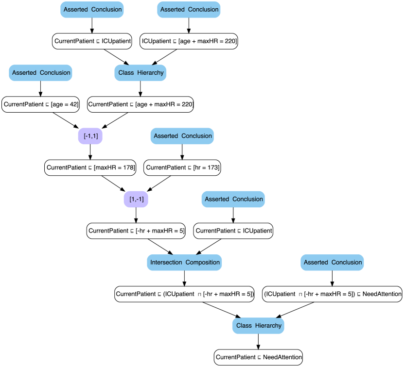
Figure 6: Showing $\textsf{{CurrentPatient}}\sqsubseteq\textsf{{NeedAttention}}$ using $\mathcal{D}_{\mathbb{Q},\textit{lin}}$

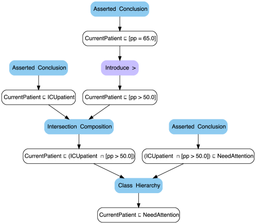
Figure 7: Showing $\textsf{{CurrentPatient}}\sqsubseteq\textsf{{NeedAttention}}$ using $\mathcal{D}_{\mathbb{Q},\textit{diff}}$

C.1 Benchmarks

In the following, we describe several ontologies that we developed to evaluate our implementation. Unfortunately, existing reasoning tasks for DLs with concrete domains, e.g. from Racer, are not expressive enough to test our algorithms; the CD values are used only as constants and do not influence the reasoning. Some of our benchmarks are scalable in the sense that they are based on similar ontologies, but one can increase their size, e.g. by increasing the number or size of axioms or constraints. All benchmarks are formulated in $\mathcal{E}\mathcal{L}_{\bot}[\mathcal{D}]$.

Simple benchmarks.

For $\mathcal{D}_{\mathbb{Q},\textit{lin}}$, there are two basic demonstration examples, Drones and Coffee. The main task in Drones is to derive the fraction of impaired sensors and propellers of a drone.

In Coffee, for different types of coffee such as cappuccino, ristretto, macchiato, etc., we define the proportions of components such as espresso, steamed milk, foam, etc. Consequently, we can identify a coffee drink based on the amounts of its components given in some unit like ml or oz.

Scalable benchmarks.

For testing the system behavior on inputs of increasing size, we provide four benchmarks, two for $\mathcal{D}_{\mathbb{Q},\textit{lin}}$ and two for $\mathcal{D}_{\mathbb{Q},\textit{diff}}$.

In Diet$(n)$, given a person’s daily consumption as a list of $n$ products and their calories from fat, protein, and carbs, we check constraints about the consumption, such as “full fat”, “full protein”, “full carbs”, “well-balanced” (55% carbs, 20% protein, 25% fat), “lower carb” (45% carbs, 25% protein, 30% fat), and “lower carb and fat” (45% carbs, 30% protein and 25% fat), expressed in $\mathcal{D}_{\mathbb{Q},\textit{lin}}$. The parameter $n$ describes the size of the linear constraints.

To scale both the DL and CD parts, we created the benchmark Artificial$(n)$ over $\mathcal{D}_{\mathbb{Q},\textit{lin}}$. With increased $n$, the number of intermediate concepts in the concept hierarchy and in proofs also increases, i.e. $A\sqsubseteq C_{\_}0\sqsubseteq\dots\sqsubseteq C_{\_}{n-1}\sqsubseteq B$. Moreover, to show each step, the concrete domain reasoner has to derive a linear constraint from $n$ given constraints. Thus, the size of a proof for $A\sqsubseteq B$ grows quadratically in $n$.

For $\mathcal{D}_{\mathbb{Q},\textit{diff}}$, there are D-Sbj$(n)$ and D-Obj$(n)$. In D-Sbj$(n)$, there is one main actor, which is a drone. The parameter $n$ quantifies the number of other objects in the world. The reasoner needs to show that all objects are at a “safe” distance from the drone.

The benchmark D-Obj$(n)$ is somehow orthogonal to D-Sbj$(n)$. The world contains $n$ drones and exactly $3$ other objects, e.g. humans or trees. Now the distances between all drones and objects are taken into consideration. Similarly to the subjective version, the reasoner needs to find out whether all objects are at “safe” distances.

Experiments.

Our findings for the $\mathcal{E}\mathcal{L}_{\bot}[\mathcal{D}]$ algorithms are summarized in Tables 1 and 2. The first two benchmarks consist of a single reasoning problem each, the remaining four represent series of small to medium-sized ontologies, for which we report ranges in each column. For the scalable benchmarks, we consider only the instances which terminated and, for each size, computed average times over three randomly generated instances of that size. The underlined benchmarks are in $\mathcal{D}_{\mathbb{Q},\textit{diff}}$, the rest in $\mathcal{D}_{\mathbb{Q},\textit{lin}}$. Columns 2–4 show the number of axioms, number of constraints, and average number of variables per constraint in the ontology, respectively. Column 5 aggregates the number of occurrences of any name (concept, role or feature) in the ontology. Columns 6–7 list the time (in ms) required for classification and proof generation, respectively, “$\mathrm{\Sigma}$” denotes the total number of instances, and “#Fin” denotes the number of instances for which proof generation finished before a timeout of 3 min.

Table 1: Results of the experiments with the $\mathcal{E}\mathcal{L}_{\bot}[\mathcal{D}]$ algorithms.

Name	Axioms	Constraints	Variables	Problem Size	Time	Proof Time	#Fin/$\mathrm{\Sigma}$
Coffee	49	21	2.3	146	329	109	1/1
Drones	93	11	2	254	195	100	1/1
Diet	26–194	15–99	2–40	81–865	61–321	45–2659	8/8
Artificial	9–24	2–13	3–5	25–144	17–347	18–	4/6
D-Sbj	55–204	20–85	1.5	191–1101	220–686	166–482	8/8
D-Obj	122–427	24–76	1.5	427–2129	315–1437	417–2099	8/8

Table 2: Supplemental experiment data for the $\mathcal{E}\mathcal{L}_{\bot}[\mathcal{D}]$ algorithms (cf. Table 1). “%DL” denotes the fraction of the reasoning time that was used by the calls to Elk. “%Incr” denotes the fraction of Elk reasoning time that would have been required for a single call to Elk on the final saturated ontology $\mathcal{O}^{\prime}$. The last two columns describe the computed proofs in terms of their tree size and “%CD”, the average fraction of the steps of the computed proof that are due to concrete domain inference steps. For the scalable benchmarks, we report either ranges or averages with standard deviations (sd) in each column.

Name	%DL(sd)	%Incr(sd)	Proof Size	%CD(sd)
Coffee	41	20	18	11
Drones	83	51	7	11
Diet	23(7)	58(6)	22–166	37(10)
Artificial	75(15)	78(16)	10–51	18(5)
D-Sbj	52(2)	76(8)	45–584	6(0)
D-Obj	63(2)	86(6)	184–1232	8(0)

References

- [1] Christian Alrabbaa, Franz Baader, Stefan Borgwardt, Patrick Koopmann, and Alisa Kovtunova. Finding small proofs for description logic entailments: Theory and practice. In LPAR, 2020. doi:10.29007/nhpp.
- [2] Christian Alrabbaa, Franz Baader, Stefan Borgwardt, Patrick Koopmann, and Alisa Kovtunova. Finding good proofs for description logic entailments using recursive quality measures. In CADE, 2021. doi:10.1007/978-3-030-79876-5_17.
- [3] Christian Alrabbaa, Franz Baader, Stefan Borgwardt, Patrick Koopmann, and Alisa Kovtunova. Combining Proofs for Description Logic and Concrete Domain Reasoning - RuleML+RR23 - Resources, 2023. doi:10.5281/zenodo.8208780.
- [4] Christian Alrabbaa, Stefan Borgwardt, Anke Hirsch, Nina Knieriemen, Alisa Kovtunova, Anna Milena Rothermel, and Frederik Wiehr. In the head of the beholder: Comparing different proof representations. In RuleML+RR, 2022. doi:10.1007/978-3-031-21541-4_14.
- [5] Christian Alrabbaa, Patrick Koopmann, and Anni-Yasmin Turhan. Practical query rewriting for DL-Lite with numerical predicates. In GCAI, 2019. doi:10.29007/gqll.
- [6] Alessandro Armando, Claudio Castellini, Enrico Giunchiglia, and Marco Maratea. A SAT-based decision procedure for the Boolean combination of difference constraints. In SAT, 2004. doi:10.1007/11527695_2.
- [7] Franz Baader, Sebastian Brandt, and Carsten Lutz. Pushing the envelope. In IJCAI, 2005. URL: http://ijcai.org/Proceedings/05/Papers/0372.pdf.
- [8] Franz Baader and Philipp Hanschke. A scheme for integrating concrete domains into concept languages. In IJCAI, 1991. URL: http://ijcai.org/Proceedings/91-1/Papers/070.pdf.
- [9] Franz Baader, Ian Horrocks, Carsten Lutz, and Ulrike Sattler. An Introduction to Description Logic. Cambridge Univ. Press, 2017. doi:10.1017/9781139025355.
- [10] Franz Baader and Jakub Rydval. Description logics with concrete domains and general concept inclusions revisited. In IJCAR, 2020. doi:10.1007/978-3-030-51074-9_24.
- [11] Franz Baader and Jakub Rydval. Using model theory to find decidable and tractable description logics with concrete domains. JAR, 66(3):357–407, 2022. doi:10.1007/s10817-022-09626-2.
- [12] Jesse L. Barlow and Erwin H. Bareiss. Probabilistic error analysis of Gaussian elimination in floating point and logarithmic arithmetic. Computing, 34(4):349–364, 1985. doi:10.1007/BF02251834.
- [13] Leonardo Mendonça de Moura and Nikolaj S. Bjørner. Z3: An efficient SMT solver. In TACAS, 2008. doi:10.1007/978-3-540-78800-3_24.
- [14] Francesco M. Donini and Fabio Massacci. ExpTime tableaux for . AIJ, 124(1):87–138, 2000. doi:10.1016/S0004-3702(00)00070-9.
- [15] Bruno Dutertre and Leonardo Mendonça de Moura. A fast linear-arithmetic solver for DPLL(T). In CAV, 2006. doi:10.1007/11817963_11.
- [16] Volker Haarslev, Ralf Möller, and Michael Wessel. The description logic extended with concrete domains: A practically motivated approach. In IJCAR, 2001. doi:10.1007/3-540-45744-5_4.
- [17] Matthew Horridge, Bijan Parsia, and Ulrike Sattler. Justification oriented proofs in OWL. In ISWC, 2010. doi:10.1007/978-3-642-17746-0_23.
- [18] Yevgeny Kazakov, Pavel Klinov, and Alexander Stupnikov. Towards reusable explanation services in Protege. In DL, 2017. URL: https://ceur-ws.org/Vol-1879/paper31.pdf.
- [19] Yevgeny Kazakov, Markus Krötzsch, and Frantisek Simancik. The incredible ELK - From polynomial procedures to efficient reasoning with ontologies. JAR, 53(1):1–61, 2014. doi:10.1007/s10817-013-9296-3.
- [20] Patrick Koopmann, Warren Del-Pinto, Sophie Tourret, and Renate A. Schmidt. Signature-based abduction for expressive description logics. In KR, 2020. doi:10.24963/kr.2020/59.
- [21] Patrick Koopmann and Renate A. Schmidt. Uniform interpolation of -ontologies using fixpoints. In FroCoS, 2013. doi:10.1007/978-3-642-40885-4_7.
- [22] Daniel Kroening and Ofer Strichman. Decision Procedures - An Algorithmic Point of View, Second Edition. EATCS. 2016. doi:10.1007/978-3-662-50497-0.
- [23] Carsten Lutz. The complexity of description logics with concrete domains. PhD thesis, 2002. URL: https://nbn-resolving.org/urn:nbn:de:hbz:82-opus-3032.
- [24] Carsten Lutz. Description logics with concrete domains - A survey. In Adv. in Modal Logic 4, 2002. URL: http://www.aiml.net/volumes/volume4/Lutz.ps.
- [25] Carsten Lutz. NExpTime-complete description logics with concrete domains. ACM TOCL, 5(4):669–705, 2004. doi:10.1145/1024922.1024925.
- [26] Boris Motik, Rob Shearer, and Ian Horrocks. Hypertableau reasoning for description logics. JAIR, 36:165–228, 2009. doi:10.1613/jair.2811.
- [27] J. Méndez, C. Alrabbaa, P. Koopmann, R. Langner, F. Baader, and R. Dachselt. Evonne: A visual tool for explaining reasoning with OWL ontologies and supporting interactive debugging. CGF, 2023. URL: https://doi.org/10.1111/cgf.14730.
- [28] Jeff Z. Pan and Ian Horrocks. Reasoning in the description logic. In DL, 2002. URL: https://ceur-ws.org/Vol-53/Pan-Horrocks-shoqdn-2002.ps.
- [29] Frantisek Simancik, Yevgeny Kazakov, and Ian Horrocks. Consequence-based reasoning beyond Horn ontologies. In IJCAI, 2011. doi:10.5591/978-1-57735-516-8/IJCAI11-187.
- [30] Peter R. Turner. Gauss elimination: Workhorse of linear algebra, 1995. NAWCADPAX-96-194-TR. URL: https://apps.dtic.mil/sti/pdfs/ADA313547.pdf.