Universal shot-noise limit for quantum metrology with local Hamiltonians
Hai-Long Shi
Innovation Academy for Precision Measurement Science and Technology,
Chinese Academy of Sciences, Wuhan 430071, China
Xi-Wen Guan
Innovation Academy for Precision Measurement Science and Technology,
Chinese Academy of Sciences, Wuhan 430071, China
Hefei National Laboratory, Hefei 230088, China
Department of Fundamental and Theoretical Physics, Research School
of Physics, Australian National University, Canberra ACT 0200, Australia
Jing Yangjing.yang@su.seNordita, KTH Royal Institute of Technology and Stockholm University,
Hannes Alfvéns vag 12, 10691 Stockholm, Sweden
Abstract
Quantum many-body interactions can induce quantum entanglement among
particles, rendering them valuable resources for quantum-enhanced sensing.
In this work, we derive a universal and fundamental bound
for the growth of the quantum Fisher information.
We apply our bound to the metrological protocol requiring only separable initial states, which can be readily prepared in experiments.
By establishing a link between our
bound and the Lieb-Robinson bound, which characterizes the operator
growth in locally interacting quantum many-body systems, we
prove that the precision cannot surpass the shot noise limit at all
times in locally interacting quantum systems.
This conclusion also holds for an initial state that is the non-degenerate
ground state of a local and gapped Hamiltonian.
These findings strongly hint that when one can only prepare separable initial states, nonlocal
and long-range interactions are essential resources for surpassing the shot
noise limit.
This observation is confirmed through numerical analysis on the long-range
Ising model.
Our results bridge the field of many-body quantum sensing
and operator growth in many-body quantum systems and open the possibility
to investigate the interplay between quantum sensing and control,
many-body physics and information scrambling.
Introduction.—Quantum entanglement is a valuable
resource in quantum information processing. In quantum metrology,
quantum Fisher information (QFI) [1, 2, 3, 4, 5, 6],
quantifying the precision of the sensing parameter, scales linearly
with the number of probes if the probes are uncorrelated, known as
the shot noise limit (SNL), also known as the standard quantum limit,
which also appears in sensing with classical resources. Quantum entanglement
can lead to a quadratic scaling known as the Heisenberg limit (HL) or
even beyond the quadratic scaling, i.e., the so-called super-HL. Entanglement
can be utilized in two ways, either in the stage of state preparation [7, 8, 9, 10, 11, 12]
or in the stage of signal sensing via the many-body interactions between
individual sensors [13, 14, 15, 16, 17],
which is the main essence of many-body quantum metrology. Recently,
the subject matter has gained renewed interest. However, the existing
protocols require to prepare the initial state in the highly entangled
Greenberger–Horne–Zeilinger (GHZ)-like states, whose preparation
is very challenging and time-consuming. One natural way to address
this issue is to combine the protocols of quantum state preparation
and quantum metrology, see e.g., Ref. [18, 19, 20],
where an entangled initial state is prepared before the sensing process.
Nevertheless, to evaluate the time cost of preparing a highly entangled
state from separable states but taking into account the restrictions
of the accessible Hamiltonians can be very challenging [21, 22, 23].
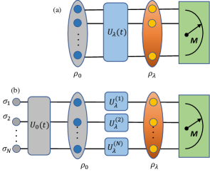
Figure 1: Comparison between our protocol (a) with the
protocol in Ref. [18] (b). In our protocol
(a), the information of the estimation parameter is encoded into the
many-body quantum states through the many-body dynamics
while in Ref. [18], the encoding dynamics
given by with
. In our protocol, the initial state is chosen to be
either a separable state or the non-degenerate ground states of a
gapped and local Hamiltonian while in Ref. [18]
the initial state is prepared through the many-body dynamics .
As such, as an alternative way to get around the overhead of quantum
state preparation, in this work we propose to prepare the probes
or sensors initially in a separable state, which can be prepared with
the current experimentally feasible technology [24, 25, 26].
In our protocol shown in Fig. 1(a), entanglement
is established in the signal sensing process due to the interactions
in the many-body sensing Hamiltonian. It is in sharp contrast with
the protocol in Ref. [18], also shown in
Fig. 1(b), where the entangled initial state
is explicitly prepared through the time evolution generated by a locally
interacting preparation Hamiltonian while the sensing Hamiltonian
is non-interacting. As we have alluded to earlier, the time cost to prepare
the entangled initial state in the protocol is difficult to estimate.
It is well known in the literature that when the initial states are
restricted to separable states, for a non-interacting sensing Hamiltonian
that is multiplicative with respective to the estimation parameter,
the precision is limited by SNL [7, 8, 9].
In our protocol, due to the many-body interactions, the state can
become entangled after the sensing process. The central question we
ask is whether many-body interactions can break the SNL? It is
also intimately related to recent studies on operator growth and
quantum chaos in quantum many-body systems [27, 28, 29, 30, 31].
To answer this question, we derive a universal bound for the growth
of the quantum Fisher information in time. Our bound can characterize
the role of quantum entanglement in information scrambling, operator
growth, and quantum chaos. We apply our bound to the quantum sensing
protocol with time-independent many-body Hamiltonians as shown in
Fig. 1(a) and estimate our bound using the celebrated
Lieb-Robinson bound [32, 33, 34, 35]
for quantum many-body systems with local interactions. We find that
it is impossible to surpass the SNL with local interactions. Such
observation is not only valid for separable initial states, but also
holds when the initial state is the non-degenerate ground state of
a locally gapped Hamiltonian, which can be experimentally prepared
by cooling. Therefore, if only separable states are accessible in
experiments, nonlocal or long-range interactions are essential to
beat the SNL and bring real quantum advantage in many-body quantum
metrology. We exemplify our findings in magnetometry with the short-range
transverse-field Ising (TFI) model, the chaotic Ising (CI) model,
and the long-range Ising (LRI) model.
Universal bound on the growth of the QFI. —We consider
the following sensing Hamiltonian
(1)
where represents the estimation parameter, and
involves interactions among sensors induced by either intrinsic interactions
or external coherent controls. In the formal case, is usually
time-independent, while in the later case, becomes time-dependent.
The generator for the quantum sensing [13, 36]
is given by
(2)
where an operator in the Heisenberg picture is defined as .
The QFI is determined by the variance of over the initial
state denoted as , i.e.,
(3)
Optimal control theory has been proposed to simultaneously optimize
the initial state and , resulting in
a bound [13, 37, 38, 15].
Here, the semi-norm is defined by the spectrum width
of an operator, i.e., the difference between its maximum eigenvalue
and minimum eigenvalue.
Eq. (3) hints that
can characterize the growth of quantum Fisher information qualitatively.
In this regard, we derive a universal bound [39]:
(4)
The saturation condition can be found
in the Supplemental Materials [39]. Alternatively, one can
rewrite
(5)
where .
A few comments in order: First, Eq. (4) is
our first main result, which holds universally for all initial states,
both time-independent and driven quantum systems. Second,
depends on the control Hamiltonian and the initial state
. Optimizing over all possible unitary
dynamics and initial states lead to
(6)
By combining this bound with ,
which can be obtained by integrating both sides of Eq. (4),
one immediately reobtains the bound given in previous works [15, 38, 37].
Compared to these studies, our bound (4)
provides a feasible approach to study the scaling behavior of the
QFI when the initial state is restricted to a specific
set of initial states.
SNL for short-range local interactions.—Here we will demonstrate
that our bound, characterizing the growth of QFI, is closely linked
to the Lieb-Robinson bound, which characterizes operator complexity
in quantum many-body with short-range local interactions. We consider
time-independent many-body Hamiltonian of the following form:
(7)
where is supported on the set with cardinality
and diameter
and representing the interactions between the spins. We require
only contains local and short-range interactions, imposing
that is independent of [35, 33, 40]
and is a local operator. Equation (7)
is the model used in magnetometry, where represents the
magnetic field [41]. We note that the bound (4)
can be written in terms of dynamic correlation matrices of local operators,
i.e.,
(8)
where
and
(9)
As indicated by Eq. (6), we observe that
implying [37, 36].
Such an HL can be saturated by utilizing GHZ-like initial states [15, 16, 13],
while also ensuring that commutes with .
As we have mentioned before, it is challenging to prepare GHZ state
experimentally and estimate the corresponding time cost theoretically.
In general, the many-body interaction can generate the entanglement
between the probes except that commutes with ,
where the states will remain separable throughout the process of signal
sensing. In this special case, the precision remains at SNL at all
times, i.e., . Generically, does not commute
with , Thus one naturally ask the question:
For separable initial states, what is the tight bound that limits
the precision? Is it possible to surpass the SNL using many-body interactions?
To address this question, we analyze the scaling of with
respect to with the Lieb-Robinson bound for local Hamiltonians [34, 32, 33, 35],
which imposes a restriction on the connected correlation functions.
Specifically, if the sensing Hamiltonian (7)
only contains local or short-range interactions, the static correlation
between two
disjoint local operators and decays exponentially,
provided the initial state is separable or the non-degenerate
ground state of some local and gapped Hamiltonians, not necessarily
the same as Eq. (7). In this case, the dynamic
correlation function also decays exponentially,
(10)
where and are constants that solely depend on
the topology of the sites, is the distance between
and , and is the celebrated Lieb-Robinson
velocity. Using Eq. (10), we demonstrate
that the scaling of is lower bounded by [39]:
(11)
where is only a function of time and independent of .
It remains finite as long as is finite and behaves as
as .
Eq. (11) is the main
result of this work. Clearly, for finite but fixed times
it implies that the QFI is limited by SNL. On the
other hand, at sufficiently long times, for time-independent systems,
one can show that is independent of time [39, 42]
and is only a function of . We further show that in [39]
the time scale to reach this regime corresponds to the case where
is much larger than the inverse of the minimum energy gap for
the system. In this regime, when is large, .
Since Eq. (11) is valid for all times and all
, combined with Eq. (4) we conclude .
Therefore, in local short-range models where operator growth is constrained
by the Lieb-Robinson bound, SNL cannot be surpassed.
The spread of the generator of the metrological bound. —
We can characterize the structure ,
the generator of the bound (4). We note that
although spreads over the lattice, the
metrological generator ,
being a sum of these non-local operators, may still remain local as
a whole, thus keeping the precision limited to the SNL. This observation
provides an alternative perspective to understand the SNL for separable
initial states in local or short-range models. A trivial example is
when commutes with while
does not commute with each individual , in which case
remains the SNL.
Now we present a non-trivial example: we assume
can be expanded in terms of two-body basis operators
(12)
where we have suppressed the time dependence for simplicity and for
spin systems is a basis spin operator,
such as while for fermionic systems
is a Hermitian basis fermionic operator,
such as or .
It should be emphasized that the number of different types of operators
indexed by are finite and does not scale with . If the
initial state is separable and
is described by fast-decaying long-range two-body interactions, i.e.,
(13)
then the SNL can not be surpassed. The proof can
be found in the Supplement Materials [39]. We can express
,
where
has support across the whole chain [39]. Essentially, the
condition (13) ensures that
does not scale with so that it behaves effectively as a local
operator, although it may have a support across the entire chain.
It is crucial to note that can be different
from , which is generically non-local.
We will further elaborate this observation with the example of magnetometry
using the TFI model.
SNL in the TFI model.—We consider the integrable TFI chain
(14)
with the periodic boundary condition ,
where . In the thermodynamic limit ,
when the ground state is ferromagnetic and degenerate,
represented by or , while
for the ground state is paramagnetic .
For any initial separable state, Eq. (4)
predicts that the QFI cannot surpass the SNL. On the other hand, this
model can be exactly solved by mapping it to a free fermion model
[43, 44] and therefore one can compute
explicitly. We show in the Supplemental Materials [39] that
indeed in this case
has the structure of Eq. (12) with
four types of ferimonic operators: ,
,
and .
The expression for the -functions, characterizing the weights
of different operators spreading from the -th site to the -th
site, can be found in [39]. In the thermodynamic limit,
behaves like for , where for ,
for , and for [39].
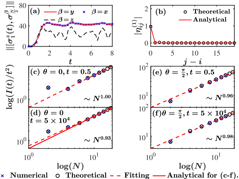
The power-law decay of -functions indicates that the evolved
operator remains extremely local, as shown in Fig. 2(b),
which ensures the condition (13), i.e.,
(15)
as Therefore, the locality of evolved operator suggests
that QFI beyond the SNL cannot be achieved by initial separable probe
states in this integrable TFL model. Fig. 2(a)
characterizes the diffusion of the correlators, suggesting that the
numerical choices of and can be considered
as the time scales for the part and full spread of local operators, respectively.
Fig. 2(c-d) numerically verify that only SNL
can be achieved for the different initial separable spin coherent
states parameterized by .
Furthermore, if we consider the initial state as the ground state of the
TFI model with known values of parameters and ,
which can be prepared by cooling. The asymptotic behavior of the QFI
with respect to the unknown parameter under the the Hamiltonian (14)
is
(16)
where the expression of -independent function is given in
the Supplemental Materials [39], confirming the claim that
only SNL can be achieved even with the ground state of local and gapped
Hamiltonians. Taking , where the ground state
becomes the spin coherent state with , we find
(17)
for and for ,
which is also verified in Fig. 2(d).
Figure 2: (a) Numerical calculation of the operator diffusion
in the TFI chain with . (b) Coefficient
characterizing the decay of the two-body interactions. (c-f) Scaling
of the QFI with respect to the number of spins at different times
for differential initial separable spin coherent states .
Here numerical data is obtained by directly diagonalizing the Hamiltonian
of the TFI model, while theoretical data is derived using results
by mapping the TFI model to the free fermion model. The analytical
result refers to Eq. (17). Other parameters used for
the calculations are , and .
SNL in the chaotic Ising model.—Different from the integrable
models, the operator complexity in chaotic models grows very rapidly [27, 28, 30, 31, 29].
Nevertheless, Eq. (4) predict
that even if the model is chaotic, where local operators are expected
to growth fast than integrable models as long as the model only contains
local interactions, the SNL cannot be surpassed by using separable
states. To see such an example, we consider the Ising model with both
transverse and longitudinal fields and the Hamiltonian is given by
(18)
where open boundary conditions are adopted. Energy-level spacing statistics
indicate that this model is quantum chaotic for [29, 45].
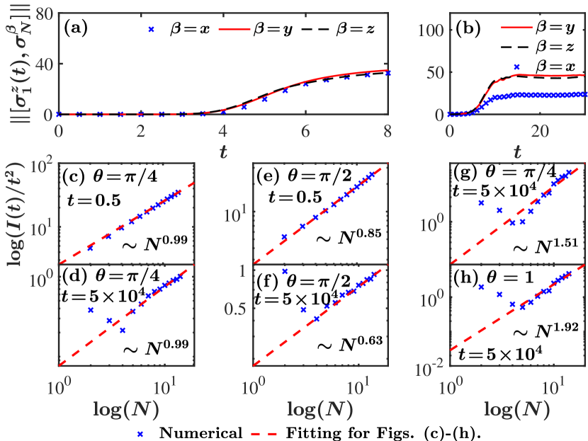
Fig. 3(c-f) verify the prediction by Eq. (11)
that separable states cannot surpass the SNL even in such chaotic
short-range systems. To surpass the SNL, we are thus motivated to
explore long-range models. The effect of quantum chaos in quantum
metrology has been studied in Ref. [46] in
the context of kick top, which is a single-spin model. Here, we show
that quantum chaos plays no role in local chaotic many-spin models.
Beyond SNL with LRI model.—As we have
shown above, it is only possible to break the SNL in long-range and
nonlocal systems, which violates the Lieb-Robinson inspired bound (11).Thus, we consider the long-range Ising model with power-law decay,
(19)
which reduces to the TFI model as For ,
this model corresponds to the Lipkin-Meshkov-Glick model [47].
In this long-range model, the breakdown of exponential
decay in connected correlation function Eq. (10)
will result in the failure of bound presented in (11).
Consequently, we expect that for small where the long-range
interactions decay sufficiently slowly, it is possible to surpass the
SNL with separable initial states. As depicted in Fig. 3(g-h),
we have identified specific instances of this scenario.
Figure 3: Numerical calculation of the operator
diffusion in (a) the CI model (b) the LRI model with . The
scaling of the QFI with respect to the number of spins at different
times for differential initial separable spin coherent states
in (c-f) the CI model and (g-h) the LRI model. Other parameters used
for the calculations are in the CI model,
and , in the LRI model.
Conclusion and outlook.—In conclusion, we have
derived a universal bound on the growth of the QFI under arbitrary
dynamics and initial states. We apply our bound to the case of separable
initial states or the non-degenerate ground state of a gapped and
local sensing Hamiltonian. We prove that with these particular set
of initial states, the QFI cannot surpass the SNL, as we have explicitly
demonstrated with TFI and CI models. This indicates that either initial entanglement or long-range interactions are essential
resource to bring the advantage of quantumness, as we have demonstrated
with the LRI.
These findings suggest an intriguing connection between operator growth
and the growth of the QFI. As such, our results shed light on many
aspects on the interplay between many-body physics, quantum control
theory, and information scrambling and open the door to investigate
many intricate questions, such as driven many-body sensing, the optimal
control metrology over a restricted set of initial states,
the connection between the growth of the QFI and the measures
characterizing quantum chaos and operator complexity. We leave these
studies for the future.
Acknowledgement. —We thank Adolfo del Campo for
useful comments on the manuscript. It is a pleasure to acknowledge
discussions with Federcio Balducci and Xingze Qiu. XWG
was supported by the NSFC key grant No. 12134015, the NSFC grant
No. 12121004, and partially supported by the Innovation Program
for Quantum Science and Technology 2021ZD0302000. JY was funded by
the Wallenberg Initiative on Networks and Quantum Information (WINQ)
and would like to thank Hui Zhai for the hospitality to host his long-term
visit at the Institute of Advanced Study in Tsinghua University, during
which this work was completed.
Notes added.—When completing this work, we noted
that a bound similar with Eq. (4) also appears in Ref. [48] with the focus on non-Hermitian sensing.
References
Helstrom [1976]C. W. Helstrom, Quantum Detection
and Estimation Theory (Academic Press, 1976).
Holevo [2011]A. S. Holevo, Probabilistic and
Statistical Aspects of Quantum Theory (Springer Science & Business Media, 2011).
Hyllus et al. [2012]P. Hyllus, W. Laskowski,
R. Krischek, C. Schwemmer, W. Wieczorek, H. Weinfurter, L. Pezzé, and A. Smerzi, Physical Review A 85, 022321 (2012).
Blumoff et al. [2022]J. Z. Blumoff, A. S. Pan,
T. E. Keating, R. W. Andrews, D. W. Barnes, T. L. Brecht, E. T. Croke, L. E. Euliss, J. A. Fast, C. A. Jackson, A. M. Jones, J. Kerckhoff, R. K. Lanza, K. Raach, B. J. Thomas, R. Velunta, A. J. Weinstein, T. D. Ladd, K. Eng, M. G. Borselli,
A. T. Hunter, and M. T. Rakher, PRX Quantum 3, 010352 (2022).
Zeng et al. [2019]B. Zeng, X. Chen, D.-L. Zhou, and X.-G. Wen, Quantum Information Meets Quantum Matter: From
Quantum Entanglement to Topological Phases of Many-Body
Systems, 1st ed. (Springer, New York, NY, 2019).
Hall [2013]B. C. Hall, “Lie groups, lie algebras, and
representations,” in Quantum Theory for Mathematicians (Springer New York, New York, NY, 2013) pp. 333–366.
Bender and Orszag [1999]C. M. Bender and S. A. Orszag, Advanced mathematical
methods for scientists and engineers I: Asymptotic methods and perturbation
theory, Vol. 1 (Springer
Science & Business Media, 1999).
Supplemental Materials
I Saturation condition of the bound
on the growth of the QFI
where denotes the average on the initial
state . Taking derivatives on both sides, we find
(S2)
Using the Cauchy-Schwarz inequality, we find
(S3)
Thus, we find
(S4)
which is equivalent to the universal bound (4)
in the main text. We define
(S5)
with initial values
(S6)
The inequality is saturated at some instant time if
(S7)
which is equivalent to
(S8)
Now we require the inequality is satisfied from the initial time
up to time , we should integrate Eq. (S8). Note
that initial time may be not appropriate to be used as the reference
point for the integration since . Instead, we
can choose a reference point such that
and then obtain
(S9)
By further considering the requirement , we can conclude
that should not change its direction as time
evolves, while exponentially increasing in its length. To satisfy
the initial condition (S6), we require that
(S10)
where
(S11)
The first condition of Eq. (S10) implies that
should vanish as . Thus we assume
as with . A straightforward analysis
show that the only possible case that is consistent with the second
equation of Eq. (S10) is . Therefore,
Eq. (S9) may be rewritten as
(S12)
To summarize, Eq. (S5) and Eq. (S9)
must be consistent. Taking derivatives on sides, we obtain the condition
for the saturation of the maximum growth rate of the QFI:
(S13)
which is obviously satisfied at .
II Analysis of the growth bound of the QFI from
Lieb-Robinson bound
It is straightforward to show that
(S14)
where is the cardinality of the support and
represents the closed neighborhood of site with a radius .
Specifically, this implies that the intersection between the sets
and is empty if and only if the site does not
belong to the closed neighborhood , i.e.,
(S15)
The first term on the right-hand side of Eq. (S14)
describes the self-correlation of local operators. The second term
accounts for the correlation between pairs of local operators that
overlap from the initial time. The last term represents the
correlation among the pairs of local operators whose supports are
initially disjoint but may overlap later due to the Lieb-Robinson
type of diffusion.
Note that , which does not scale with .
As a result, we find that
(S16)
and
(S17)
On the other hand, if , then the set
and are disjoint, allowing us to estimate
by using the Lieb-Robinson bound (10).
Consequently, we find [34, 32, 33, 35],
(S18)
which holds for initial separable states or the non- degenerate ground
state of local and gapped Hamiltonians. Here, is
the distance connecting the set with the set ,
is a constant that solely depends on the topology of the sites, and
is the celebrated Lieb-Robinson velocity. By substituting
Eqs. (S16-S18) into Eqs. (S14),
we find
(S19)
where is a function of only time, independent of ,
and we have used the results and .
III Proof of being
time-independent for time-independent Hamiltonians
For time-independent Hamiltonians , the
generator for quantum sensing , Eq. (2) is given
by
(S20)
By using the Baker–Campbell–Hausdorff formula [49],
the above equation can be rewritten as
(S21)
where the Liouvillian is defined as
whose eigenvalues are and
(S22)
By the Choi-Jamiokowski isomorphism, we can rewrite operator
as a vector in the space
where is the original Hilbert space. Due to the Hermiticity
of , we can assume that it can be diagonalized as
so that
(S23)
We observe that in the limit
(S24)
Therefore, we conclude
(S25)
which is time-independent. Apparently, the condition to reach this
limit is
(S26)
which is the minimum energy gap of the system. Since
then we can assume for sufficient long-time
and large .
IV Proof of the SNL for fast-decaying
two-body metrological operator
Then it is straightforward to verify that
(S27)
So one can find
(S28)
where is defined in the main text. To facilitate
the following discussions, we also introduce
(S29)
Then it is straightforward to show that
(S30)
where is a separable state. Thus, we find
(S31)
where and
(S32)
Our aim is to show that
(S33)
which suggests that SNL cannot be surpassed by separable states. To
show Eq. (S33), it suffices to demonstrate that
(S34)
Due to we have
(S35)
as where can be any state and not
restricted to separable states. Also, by using the Cauchy-Schwartz
inequality, we can show that as
(S36)
Furthermore, we have the following condition to characterize the locality
of the fast decay operator:
(S37)
where
(S38)
Apparently
(S39)
In the limit, and , Euler-Maclaurin formula
allows us to rewrite the series on r.h.s. of Eq. (S38)
in terms of a double integral
which is easier to evaluate than the double series.
Now we are in a position to show that
(S40)
where we have utilized Eq. (S36) in the first
inequality, Eq. (S39) in the second inequality,
and the fact that the number of terms of the sum over is
finite in the last inequality. Next, we will discuss two cases where
the is two-body spin or fermionic operators, respectively,
to show that
(S41)
IV.1 Two-body spin operators
When and
are two-body spin operators, we note that if does not
overlap with then the correlation is zero since
is a separable state. With this observation, we find
(S42)
where the appearance of in the first equality comes
from the initial state is restricted to separable states. Using (S39)
,
If we do not require separable initial states then
(S43)
which suggests that
is not guaranteed since
may not be bounded given Eqs. (S37) and (S38).
Actually, the HL can be achieved for GHZ-like entangled initial states
and thus Eq. (S34) is not expected to hold.
IV.2 Two-body fermionic operators
When and
are two-body fermionic operators, see the below:
(S47)
(S51)
(S55)
which suggests that if
then
Thus, we can find
(S56)
Using the condition that the initial state is separable, one can replace
in above summation with , leading to
(S57)
Thus, we find
Taking and and using Eq. (S37),
we prove Eq. (S41).
V Metrological generator for the TFI periodic chain
The integrable Ising model Eq. (14)
can be diagonalized as a free fermion model [43, 44].
Defining ,
we can construct fermion creation and annihilation operators by the
Jordan-Wigner transformation:
(S58)
The inverse transformation is then given by
(S59)
In terms of fermionic operators, the Hamiltonian can be expressed
as
(S60)
where is
the parity operator commuting with the Hamiltonian. Thus, the above
Hamiltonian can be rewritten according to the parity symmetry, i.e.,
where “odd” and “even” correspond to the Hamiltonian acting
on the subspaces of the Fock space with an odd or even number of fermions,
which is also related with periodic () or antiperiodic ()
boundary conditions.
It can be shown that
at the thermodynamic limit . Thus, for convenience, we
work on the subspace with an even number of fermions. Introducing
the Fourier transformation
(S61)
and the Bogoliubov fermions
(S62)
the Hamiltonian reduces to the diagonalized form
(S63)
where and
is determined by
(S64)
In terms of and ,
can be expressed as
(S65)
Thus, we obtain
(S66)
By using Eq. (S62), the Eq. (S66)
can be expressed as
(S67)
where
(S68)
By further using the Fourier transformation (S61),
we obtain
(S69)
where
(S70)
and is the Fourier transformation of the function
, i.e.,
(S71)
We can further rewrite Eq. (S70) in terms of Eq. (12)
in the main text, i.e.,
(S72)
where we have suppressed the time-dependence, ,
,
and .
The corresponding -functions are given by
(S73)
The expressions for , ,
and are dramatically simplified in the limit
and . In the limit, , we can rewrite
as an integral
(S74)
By the Riemann-Lebesgue lemma [50], the last
integral in the right hand of Eq. (S74) tends to zero as
. The second integral in the right hand of Eq. (S74)
can be evaluated by introducing :
(S75)
where the contour is along the counterclockwise direction
of the unit circle on the complex plane.
We denote ,
where
(S76)
The residues of are listed as follows:
(S77)
Then, by using the residue theorem, we obtain
for ,
for , and
for . Finally, we have
(S78)
(S79)
(S80)
Similarly, we can obtain the other terms under the limit
and
(S87)
(S91)
(S98)
(S102)
and .
VI QFI for the short-range TFI model
According to Eq. (S66), the generator
given in Eq. (2) of the integrable Ising model is given
by
For the numerical calculation of QFI, we need to express in
the spin representation. Thus, by using Eq. (S62)
and (S61), we can rewrite Eq. (S103)
as
(S104)
where
(S105)
and is the Fourier transformation of
the function like Eq. (S71). Equations
(S104), (S105), and (S55) provide
a numerical approach to express in terms of the spin operators.
Finally, QFI can be easily calculated by using ,
Eq. (3).
Now we consider a special case where the initial state
is chosen to be the paramagnetic product state ,
which can be viewed as the ground state of the Ising chain
(14) by taking
and we denote it as . We denote the Bogoliubov
fermionic operators and the Bogoliubov angle of
by and , respectively. We now consider
the QFI for the evolved state with respect
to the parameter where .
Here we focus on the long-time limit and thus Eq. (S103)
reduces to
(S106)
where and we use the
result for .
A constant is ignored in the last equation since it does not affect
the value of QFI. It can be checked that the ground state
can be expressed as
(S107)
where is a normalization factor,
is the ground state of Hamiltonian , and
(S108)
Then we have
(S109)
where
we use the results .
Substituting Eqs. (S64), (S108), and (S109)
into the definition of QFI, we obtain
(S110)
In the thermodynamic limit , the above equation becomes
(S111)
where the contour is the the unit circle on the complex
plane and . Finally, by using the residue theorem, we obtain
(S112)
Since the ferromagnetic product state
is the ground state by taking ,
then we obtain