ABSTRACT

Multichannel active noise control (MCANC) is widely utilized to achieve significant noise cancellation area in the complicated acoustic field. Meanwhile, the filter-x least mean square (FxLMS) algorithm gradually becomes the benchmark solution for the implementation of MCANC due to its low computational complexity. However, its slow convergence speed more or less undermines the performance of dealing with quickly varying disturbances, such as piling noise. Furthermore, the noise power variation also deteriorates the robustness of the algorithm when it adopts the fixed step size. To solve these issues, we integrated the normalized multichannel FxLMS with the momentum method, which hence, effectively avoids the interference of the primary noise power and accelerates the convergence of the algorithm. To validate its effectiveness, we deployed this algorithm in a multichannel noise control window to control the real machine noise.

.   ntroduction

Active noise control (ANC) is a technique that utilizes the loudspeaker generating "anti-noise" wave with the negative amplitude of the unwanted noise to cancel this acoustic disturbance [1, 2, 3, 4]. Compared to passive noise cancellation strategy, such as the noise barrier, ANC exhibits more effectiveness in mitigating the low-frequency noise without occupying large space, affecting air ventilation, and destroying the natural environment. Hence, the ANC technique is widely applied in many different fields, including the headphones [5], windows [6, 7, 8, 9, 10, 11, 12], and the open space [13]. However, in many real scenario, ANC can only achieve the local noise control around the error sensor [14]. To enlarge the size of the noise reduction area, the multichannel ANC (MCANC) is usually applied at the expense of the system complexity [15].

With the significant development of powerful processors and other digital devices [16], such as digital signal processors, analog-to-digital converters (ADC), and digital-to-analog converters (DAC), it becomes feasible to realize the active control with adaptive algorithms [17, 18]. Among these algorithms, the filtered-x least mean square (FxLMS) algorithm is prevalent in various applications since its low computational complexity [19]. Besides, it utilizes a filtered reference signal to update the control filter and compensates for the delay involved by the secondary path, which enhances the system robustness. Since its satisfactory performance in the single-channel ANC, FxLMS is also extended to the multichannel FxLMS (McFxLMS) algorithm while maintaining similar advantages in the MCANC application [20]. Meanwhile, some other FxLMS-based algorithms have been proposed to further reduce computations [21, 22], improve convergence [23, 24], or cope with the output saturation issue [25, 26, 27, 28, 29, 30].

Nevertheless, these FxLMS-based algorithms are always haunted by a practical issue [31]: the step size bound is sensitive to the reference signal’s power. An inappropriate step-size selection usually results in the divergence or slow convergence problem. For the same reason, the stability of the McFxLMS algorithm will be deteriorated in canceling the varying noise when its step size is chosen as a constant. To solve this issue, the variable step-size methods seem to be an effective strategy. However, most of these variable step-size mechanisms will severely aggravate the computational load, especially for the multichannel system. Under this situation, the multichannel normalized FxLMS (MNFxLMS) algorithm [32, 33] becomes a better choice because it can avoid the influence of input power by pre-whitening the referenced signal while slightly increasing computations. In that, MNFxLMS is undoubtedly suitable to deal with the primary noise with a massive power variation over time. To further improve its convergence, we integrate the momentum technique to MNFxLMS in this paper. In the new algorithm, the momentum term [34, 35, 36] accumulates the previous gradient information to accelerate the convergence of MNFxLMS, which hence, leads to a satisfactory noise reduction performance when dealing with the quick-varying noise. The momentum MNFxLMS also smooths the varied gradient and reduces the high-frequency disturbance on the control filter’s weight. Furthermore, this paper carries out the simulations on the proposed algorithm, which is used to deal with real quick-varying noise in measured paths.

This paper is organized as the following descriptions: Section 2 revisits the multichannel normalized FxLMS algorithm; Section 3 proposes the momentum MNFxLMS algorithm and addresses a brief analysis. Section 4 exhibits the simulation results of the McFxLMS, MNFxLMS, and momentum MNFxLMS algorithms, and Section 5 summaries the whole paper.

.   he Multichannel Normalized Filtered-x LMS algorithm

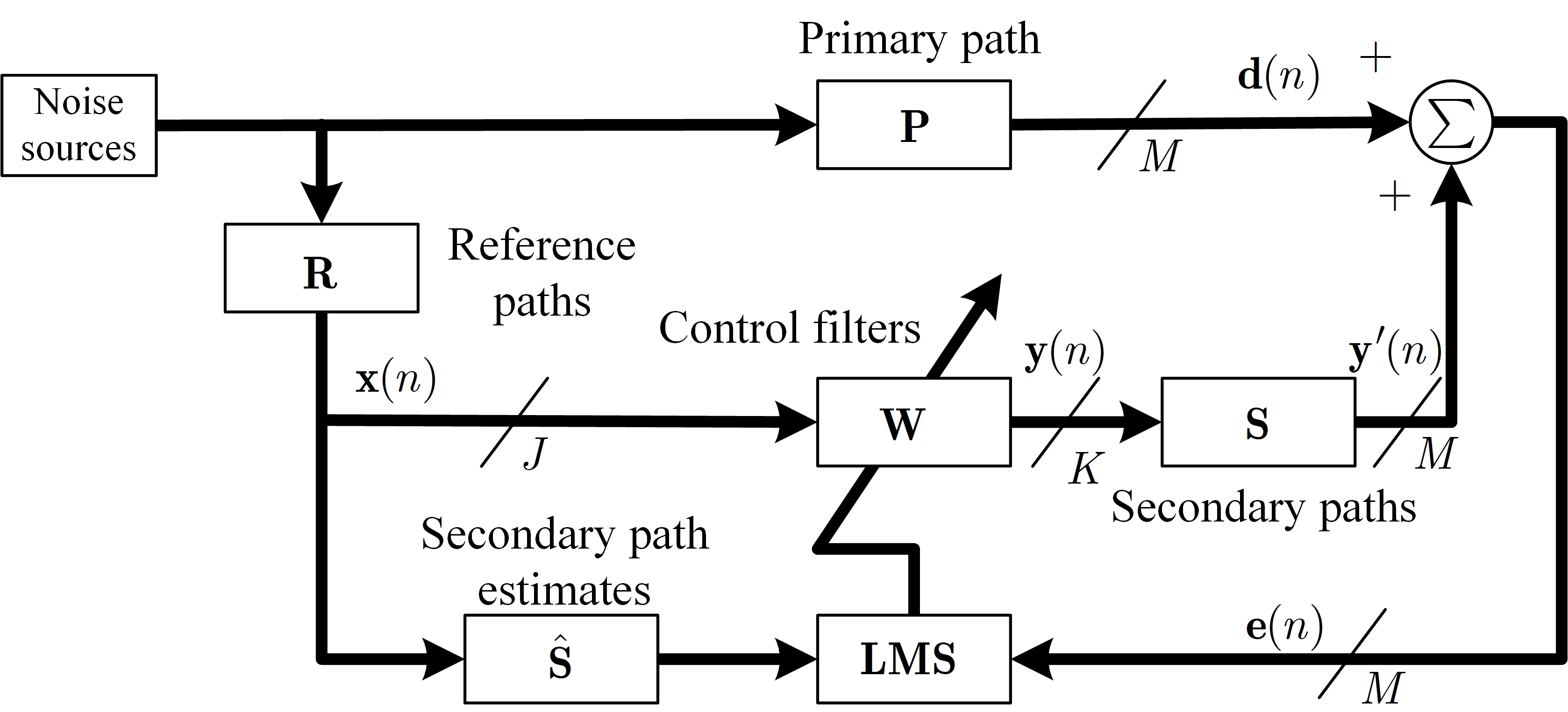
Figure 1: Block diagram of a multichannel ANC with $J$ microphones, $K$ secondary sources, and $M$ error microphones [37].

In this paper, we consider a $J\times K\times M$ multichannel active noise control (MCANC) system, which uses $J$ reference microphones and $K$ secondary sources to cancel the disturbances at $M$ error microphones, as shown in Figure 1. In this figure, $\mathbf{P}$, $\mathbf{W}$, and $\mathbf{S}$ denote the transfer functions of the primary paths, control filters, and secondary paths, respectively. $\mathbf{\hat{S}}$ stands for the estimate of $\mathbf{S}$ and is obtained through the offline system identification.

The control signal of the $k$th secondary source can be expressed as

$$y_{\mathrm{k}}(n)=\sum^{\mathrm{J}}_{\mathrm{j=1}}\mathbf{w}^{\mathrm{T}}_{\mathrm{kj}}(n)\mathbf{x}_{\mathrm{j}}(n)$$ (1)

where $\mathbf{w}_{\mathrm{kj}}(n)$ denotes the $kj$th control filter that models the $j$th reference to drive the $k$th secondary source and is expressed as

$$\mathbf{w}_{\mathrm{kj}}(n)=\begin{bmatrix}w_{\mathrm{kj,1}}(n)&w_{\mathrm{kj,2}}(n)&\cdots&w_{\mathrm{kj,N}}(n)\end{bmatrix}^{\mathrm{T}}\in\mathbb{R}^{\mathrm{N\times 1}}$$

which has $N$ taps, and $\mathbf{x}_{\mathrm{j}}(n)$ is the $j$th reference vector give by

$$\mathbf{x}_{\mathrm{j}}(n)=\begin{bmatrix}x_{\mathrm{j}}(n)&x_{\mathrm{j}}(n-1)&\cdots&x_{\mathrm{j}}(n-N-1)\end{bmatrix}^{\mathrm{T}}\in\mathbb{R}^{\mathrm{N\times 1}}.$$

$\mathrm{T}$ and $\mathbb{R}$ represent the transpose operation and the real number, respectively. The error signal at the $m$th microphone can be written as

$$e_{\mathrm{m}}(n)=d_{\mathrm{m}}(n)+\sum^{\mathrm{K}}_{\mathrm{k=1}}y_{\mathrm{k}}(n)*s_{\mathrm{mk}}(n)$$ (2)

where $\ast$ denotes the linear convolution, and $s_{\mathrm{mk}}(n)$ stands for the secondary path from the $k$th secondary source to the $m$th error microphone.

Based on the principle of the minimal disturbance [33], we define an increment of the $kj$th control filter at the $n+1$ iteration as

$$\delta\mathbf{w}_{\mathrm{kj}}(n+1)=\mathbf{w}_{\mathrm{kj}}(n+1)-\mathbf{w}_{\mathrm{kj}}(n)$$ (3)

and an equality constrain as

$$d_{\mathrm{m}}(n)+\sum^{\mathrm{J}}_{\mathrm{j=1}}\sum^{\mathrm{K}}_{\mathrm{k=1}}\mathbf{w}^{\mathrm{T}}_{\mathrm{kj}}(n+1)\mathbf{x^{\prime}}_{\mathrm{jkm}}(n)=0$$ (4)

where $\mathbf{x^{\prime}}_{\mathrm{jkm}}(n)$ represents the $jkm$th filtered reference signal obtained from

$$\mathbf{x^{\prime}}_{\mathrm{jkm}}(n)=\mathbf{x}_{\mathrm{j}}(n)*s_{\mathrm{mk}}(n)\in\mathbb{R}^{\mathrm{N\times 1}}.$$ (5)

To solve Equation 3 and Equation 4, we construct a Lagrange function as

$$J(n)=\sum^{\mathrm{J}}_{\mathrm{j=1}}\sum^{\mathrm{K}}_{\mathrm{k=1}}\big{\|}\delta\mathbf{w}_{\mathrm{kj}}(n+1)\big{\|}^{2}+\sum^{\mathrm{M}}_{\mathrm{t=1}}\lambda_{\mathrm{t}}\left[d_{\mathrm{t}}(n)+\sum^{\mathrm{J}}_{\mathrm{j=1}}\sum^{\mathrm{K}}_{\mathrm{k=1}}\mathbf{w}^{\mathrm{T}}_{\mathrm{kj}}(n+1)\mathbf{x^{\prime}}_{\mathrm{jkt}}(n)\right]$$ (6)

where $\|\cdot\|$ and $\lambda_{\mathrm{t}}$ denote the 2-norm and the $t$th Lagrange multiplier, respectively.

According to the Lagrange multiplier method [33], we derive the solution to minimize Equation 6 as the following procedures:

(1). The gradient of Equation 6 with respect to $\mathbf{w}_{\mathrm{kj}}(n+1)$ is derived as

$$\frac{\partial J(n)}{\partial\mathbf{w}_{\mathrm{kj}}(n+1)}=2\left[\mathbf{w}_{\mathrm{kj}}(n+1)-\mathbf{w}_{\mathrm{kj}}(n)\right]+\sum^{\mathrm{M}}_{\mathrm{t=1}}\lambda_{\mathrm{t}}\mathbf{x^{\prime}}_{\mathrm{jkt}}(n).$$ (7)

Setting Equation 7 to $\mathbf{0}$ yields

$$\mathbf{w}_{\mathrm{kj}}(n+1)=\mathbf{w}_{\mathrm{kj}}(n)-\frac{1}{2}\sum^{\mathrm{M}}_{\mathrm{t=1}}\lambda_{\mathrm{t}}\mathbf{x^{\prime}}_{\mathrm{jkt}}(n)$$ (8)

(2). By substituting Equation 8 into Equation 4:

$$d_{\mathrm{m}}(n)=-\sum^{\mathrm{J}}_{\mathrm{j=1}}\sum^{\mathrm{K}}_{\mathrm{k=1}}\left[\mathbf{w}_{\mathrm{kj}}(n)-\frac{1}{2}\sum^{\mathrm{M}}_{\mathrm{t=1}}\lambda_{\mathrm{t}}\mathbf{x^{\prime}}_{\mathrm{jkt}}(n)\right]^{\mathrm{T}}\mathbf{x^{\prime}}_{\mathrm{jkm}}(n)$$ (9)

we can obtain

$$e_{\mathrm{m}}(n)=\frac{1}{2}\sum^{\mathrm{J}}_{\mathrm{j=1}}\sum^{\mathrm{K}}_{\mathrm{k=1}}\sum^{\mathrm{M}}_{\mathrm{t=1}}\lambda_{\mathrm{t}}\mathbf{x^{\prime}}^{\mathrm{T}}_{\mathrm{jkt}}(n)\mathbf{x^{\prime}}_{\mathrm{jkm}}(n)\approx\frac{1}{2}\sum^{\mathrm{J}}_{\mathrm{j=1}}\sum^{\mathrm{K}}_{\mathrm{k=1}}\lambda_{\mathrm{m}}\big{\|}\mathbf{x^{\prime}}_{\mathrm{jkm}}(n)\big{\|}^{2}$$ (10)

where it is assumed that $\mathbf{x^{\prime}}_{\mathrm{jkt}}(n)$ and $\mathbf{x^{\prime}}_{\mathrm{jkm}}(n)$ are orthogonal ($t\neq m$) [32]. Hence, from Equation 10, the Lagrange multiplier is derived as

$$\lambda_{\mathrm{m}}=\frac{2e_{\mathrm{m}}(n)}{\sum^{\mathrm{J}}_{\mathrm{j=1}}\sum^{\mathrm{K}}_{\mathrm{k=1}}\big{\|}\mathbf{x^{\prime}}_{\mathrm{jkm}}(n)\big{\|}^{2}}.$$ (11)

(3). Substituting Equation 11 into Equation 8 yields

$$\mathbf{w}_{\mathrm{kj}}(n+1)=\mathbf{w}_{\mathrm{kj}}(n)-\sum^{\mathrm{M}}_{\mathrm{m=1}}\frac{e_{\mathrm{m}}(n)}{\sum^{\mathrm{J}}_{\mathrm{j=1}}\sum^{\mathrm{K}}_{\mathrm{k=1}}\big{\|}\mathbf{x^{\prime}}_{\mathrm{jkm}}(n)\big{\|}^{2}}\mathbf{x^{\prime}}_{\mathrm{jkm}}(n).$$ (12)

To control the magnitude of the increment of the control filter, we introduce a positive multiplier $\widetilde{\mu}~{}(0<\widetilde{\mu}<1)$ in Equation 12:

$$\mathbf{w}_{\mathrm{kj}}(n+1)=\mathbf{w}_{\mathrm{kj}}(n)-\widetilde{\mu}\sum^{\mathrm{M}}_{\mathrm{m=1}}\frac{e_{\mathrm{m}}(n)\mathbf{x^{\prime}}_{\mathrm{jkm}}(n)}{\sum^{\mathrm{J}}_{\mathrm{j=1}}\sum^{\mathrm{K}}_{\mathrm{k=1}}\big{\|}\mathbf{x^{\prime}}_{\mathrm{jkm}}(n)\big{\|}^{2}+\varepsilon}$$ (13)

where $\varepsilon$ is a small positive scalar to guarantee the division result within the finite value. Equation 13 is so-call multichannel normalized filtered-x least mean square (MNFxLMS) algorithm [32]. Equation 13 can be rewritten as

$$\mathbf{w}_{\mathrm{kj}}(n+1)=\mathbf{w}_{\mathrm{kj}}(n)-\sum^{\mathrm{M}}_{\mathrm{m=1}}\mu_{\mathrm{m}}(n)e_{\mathrm{m}}(n)\mathbf{x^{\prime}}_{\mathrm{jkm}}(n)$$ (14)

where the equivalent step size of the MNFxLMS algorithm is given by

$$\mu_{\mathrm{m}}(n)=\frac{\widetilde{\mu}}{\sum^{\mathrm{J}}_{\mathrm{j=1}}\sum^{\mathrm{K}}_{\mathrm{k=1}}\big{\|}\mathbf{x^{\prime}}_{\mathrm{jkm}}(n)\big{\|}^{2}+\varepsilon}$$ (15)

which is inversely proportional to the power of the reference signal. Therefore, the MNFxLMS algorithm effectively avoids the influence of input power variation and enforces the adaptive algorithm’s robustness.

.   he Momentum MNFxLMS algorithm

To further fasten the convergence of the MNFxLMS algorithm, we integrate the momentum mechanism [34, 35, 36] into the updating equation of Equation 13 as

$$\mathbf{w}_{\mathrm{kj}}(n+1)=\mathbf{w}_{\mathrm{kj}}(n)-\eta_{\mathrm{kj}}(n)$$ (16)

where $\eta_{\mathrm{kj}}(n)$ denotes the momentum of the algorithm given by

$$\eta_{\mathrm{jk}}(n)=\gamma\cdot\eta_{\mathrm{kj}}(n-1)+\widetilde{\mu}\sum^{\mathrm{M}}_{\mathrm{m=1}}\frac{e_{\mathrm{m}}(n)\mathbf{x^{\prime}}_{\mathrm{jkm}}(n)}{\sum^{\mathrm{J}}_{\mathrm{j=1}}\sum^{\mathrm{K}}_{\mathrm{k=1}}\big{\|}\mathbf{x^{\prime}}_{\mathrm{jkm}}(n)\big{\|}^{2}+\varepsilon}.$$ (17)

In Equation 17, $\gamma\in\left(0,1\right)$ stands for the forgetting factor, which decides the degree of the influence of previous gradients on the weight increment. Since the momentum term of Equation 17 accumulates the previous gradients, it is evident that the convergence of the proposed algorithm will be significantly accelerated if these gradients have the same direction.

It is worth noting that the z-transform expression of Equation 17 can be written as

$$H(z)=\frac{1}{1-\gamma z^{-1}}\Delta(z)$$ (18)

where $H(z)$ and $\Delta(z)$ represent the z-transform of $\eta(n)$ and the last term in the left side of Equation 17, respectively. The magnitude response of Equation 18 is shown in Figure 2. It can figure out that, for the quick-varying gradient, the momentum term works like a low-pass filter, which attenuates the high-frequency disturbance on the control filter’s weights. However, for the low-frequency varied gradient, its amplitude will be amplified so that to improve the convergence of the algorithm.

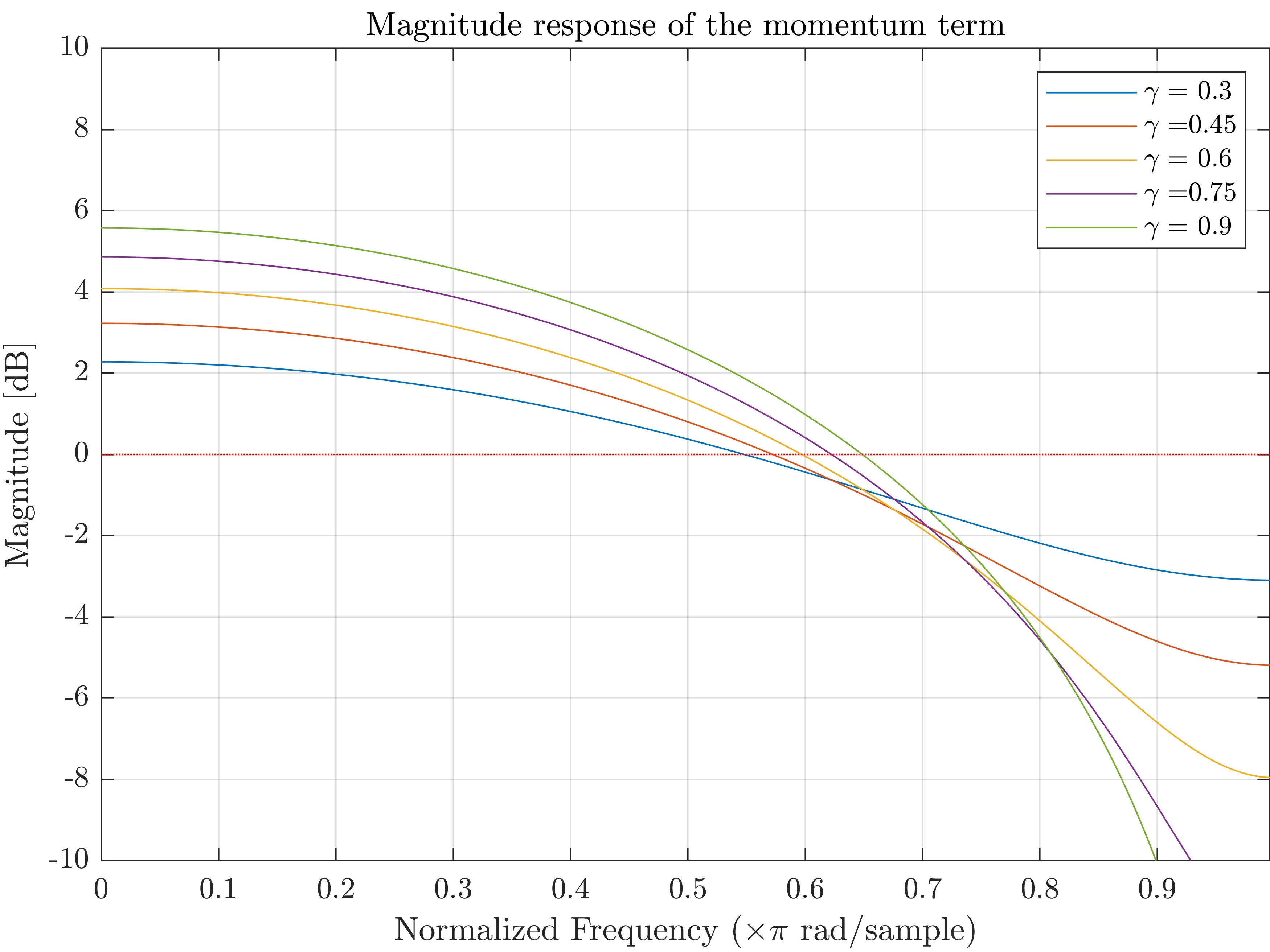
Figure 2: Magnitude response of the momentum function with different values of the forgetting factor $\gamma$.

.   imulation result

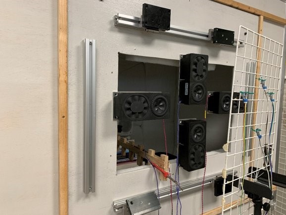
Figure 3: The front view of a $4$-channel active noise control system, which has $1$ reference microphone, $4$ secondary source and $4$ error sensors.

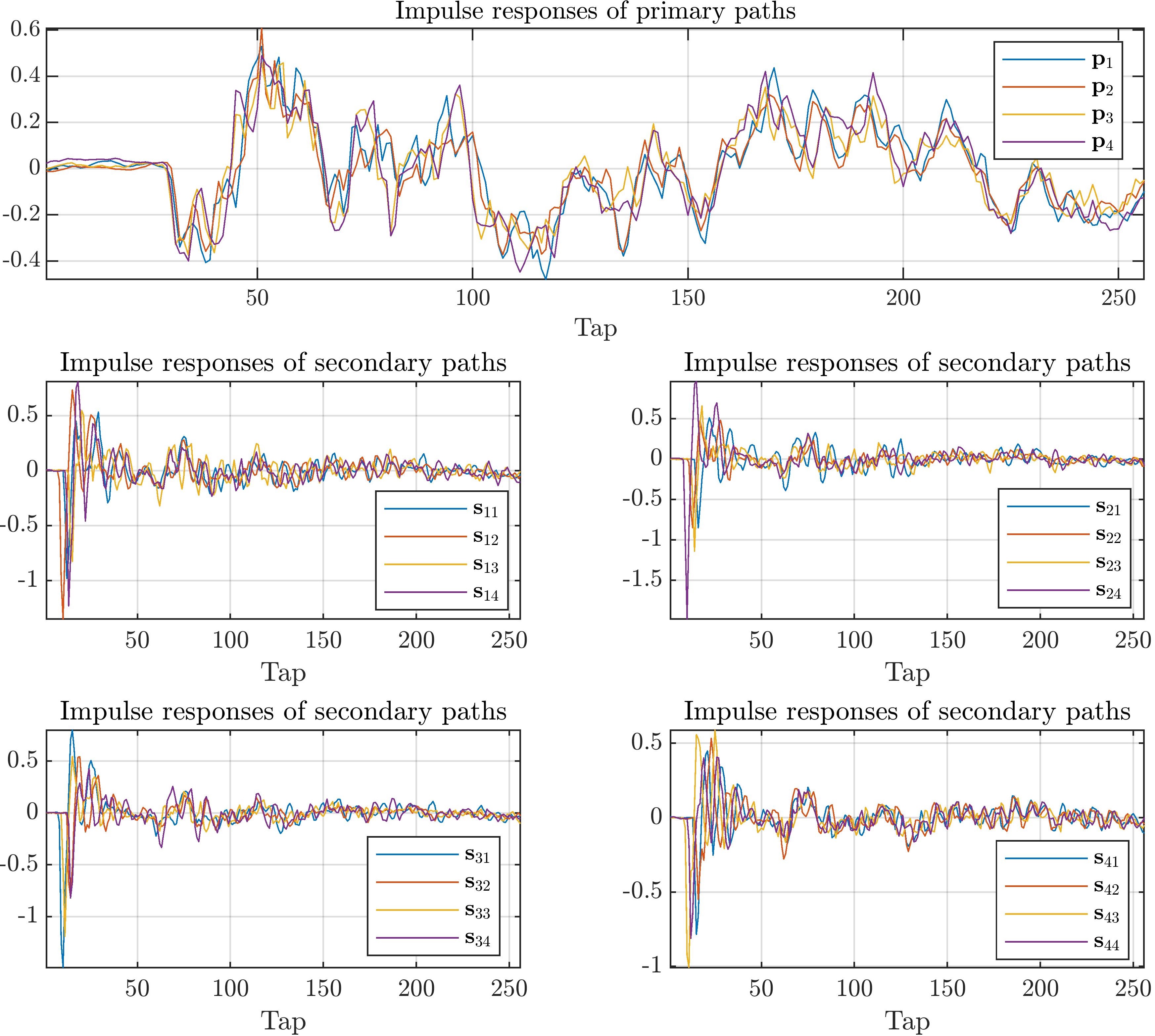
Figure 4: Impulse responses of primary paths and secondary paths: $\mathbf{p}_{\mathrm{j}}$ denotes the path from the primary source to the $j$th error microphone; $\mathbf{s}_{\mathrm{mk}}$ represents the secondary path form the $k$th secondary source to the $m$th error microphone, and $j,k,m=1,2,3,4$.

To carry out the simulations on the McFxLMS, MNFxLMS, and momentum MNFxLMS algorithms, we measured the primary and secondary paths from a 4-channel ANC system installed in a noise chamber, as shown in Figure 3. This wooden chamber has a dimension of $1.2~{}\text{m}\times 1.2~{}\text{m}\times 1.2~{}\text{m}$ and a aperture with the size of $60~{}\text{cm}\times 50~{}\text{cm}$ at its facade. A noise source is placed inside the chamber and put $1\text{m}$ way from the aperture, which has four secondary mounted around its frame. There are four error microphones fixed in a grid kept $50~{}\text{cm}$ away from the secondary sources. The reference microphone of this MCANC system is placed close to the noise source. The impulse responses of measured primary and secondary paths are illustrated in Figure 4.

Furthermore, the control filter and secondary path estimate in all algorithms have $512$ and $256$ taps, respectively. The forgetting factor of the momentum MNFxLMS algorithm is set to $0.9$.

4.1.   The cancellation of varying broadband noise

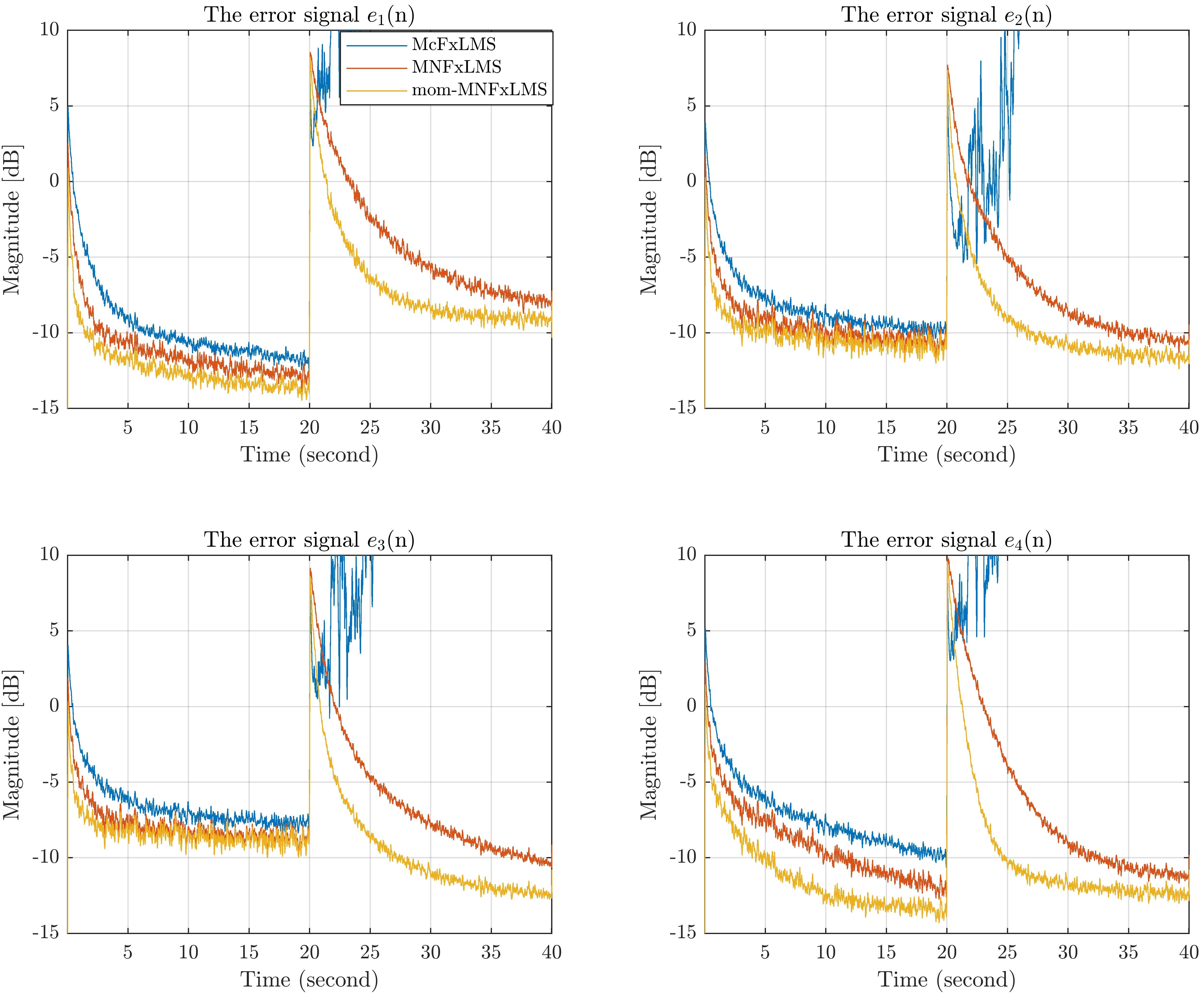
Figure 5: Time histories of error signals at the four error microphones. The step size of the McFxLMS algorithm is set to $0.000001$, and step sizes of the MNFxLMS and momentum MNFxLMS algorithms are set to $0.001$. The forgetting factor of $\gamma$ is $0.9$.

In the first simulation, the 4-channel ANC system is utilized to cancel the broadband noise. In the first $20$ seconds, the broadband noise has the frequency of $200$ to $800$ Hz and the amplitude of $10$ dB; in the next $20$ seconds, the amplitude of this noise changes to $15$ dB, and its frequency becomes $100$ to $1600$ Hz.

During the simulation, the McFxLMS algorithm has a step size of $0.000001$, while the step sizes of the MNFxLMS and momentum MNFxLMS are set to $0.001$. Figure 5 exhibits the four error signal’s waveform of the algorithms. From this result, it can be found that the McFxLMS algorithm diverges when it meets the large input power. Meanwhile, the MNFxLMS and momentum MNFxLMS algorithm can remain a satisfactory converge even though the primary noise has a significant variation. It is because the step size in MNFxLMS will automatically adjust with the input power, as shown in Equation 15. Furthermore, with the assistance of the gradient accumulation, the momentum MNFxLMS algorithm shows a faster convergence behavior than the conventional MNFxLMS.

4.2.   The cancellation of a real piling noise

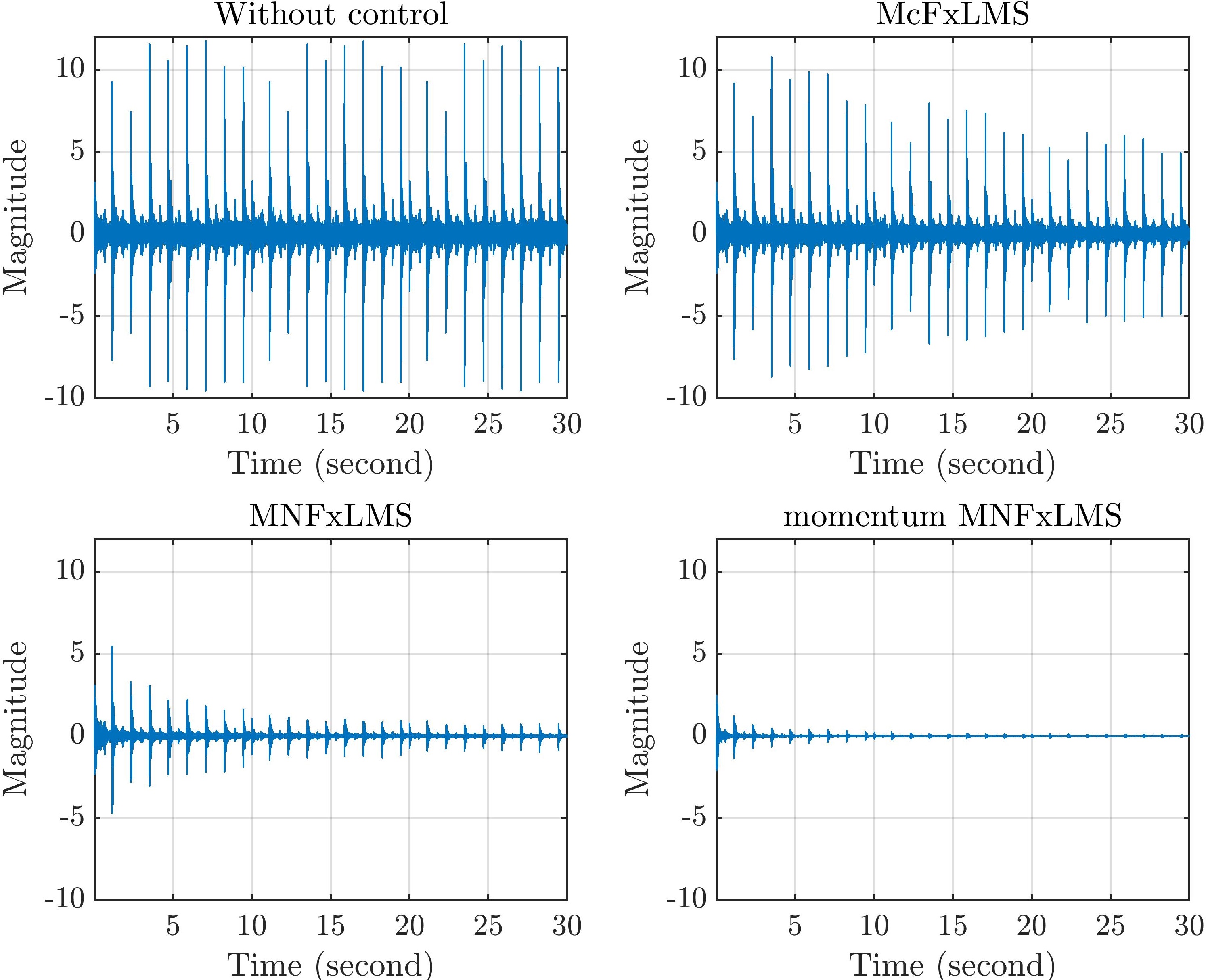
Figure 6: Time history of a real piling noise at the first error microphone. The step size of the McFxLMS algorithm is set to $0.0001$, and the step sizes of the MNFxLMS and momentum MNFxLMS algorithms are set to $0.001$. The forgetting factor of $\gamma$ is $0.9$.

In the second simulation, the primary noise becomes a real piling noise, as shown in Figure 6. To ensure the convergence of the McFxLMS algorithm, its step size is set to $0.0001$ at the expense of its convergence speed. Meanwhile, the MNFxLMS and momentum MNFxLMS can have a greater step size of $0.001$. Under this situation, the momentum MNFxLMS algorithm achieves the fastest convergence among these algorithms, as illustrated in Figure. 6. However, all these three algorithms obtain similar noise reduction levels around $20$ dB at the steady-state.

4.3.   The cancellation of an fMRI noise

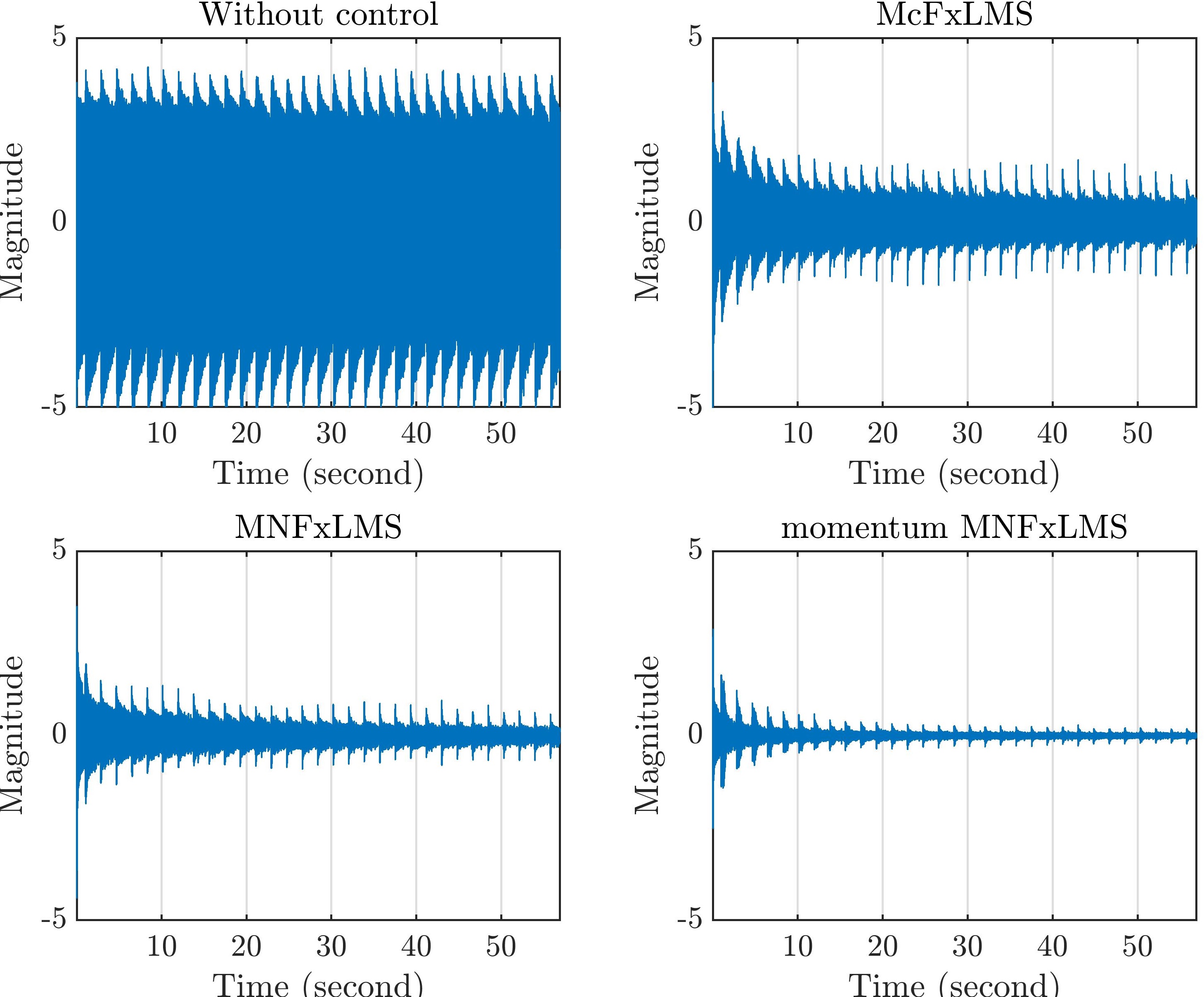
Figure 7: Time history of an fMRI noise at the first error microphone. The step size of the McFxLMS algorithm is set to $0.0001$, and the step sizes of the MNFxLMS and momentum MNFxLMS algorithms are set to $0.01$. The forgetting factor of $\gamma$ is $0.9$.

In the final simulation, the primary noise is a real functional magnetic resonance imaging (fMRI) machine noise [38], as shown in Figure 6. To ensure the convergence of the McFxLMS algorithm, its step size is set to $0.0001$. The MNFxLMS and momentum MNFxLMS algorithms have a step size of $0.001$. Under this situation, the momentum MNFxLMS algorithm achieves the fastest convergence among these algorithms, as illustrated in Figure. 6. All these three algorithms obtain similar noise reduction levels around $21.2$ dB at the steady-state.

.   onclusions

To assist the multichannel active noise control (MCANC) system in canceling quick-varying noise, the paper integrates the momentum method with the multichannel normalized filtered-x least mean square (MNFxLMS) algorithm. The MNFxLMS algorithm avoids the input power’s influence on the step size bound, and the momentum method accelerates the convergence by accumulating the previous gradient information. The momentum MNFxLMS algorithm combines these two advantages and hence, exhibits a satisfactory performance in canceling the quick-varying noise. The simulation on the measured paths of a 4-channel ANC system verifies the effectiveness of the proposed algorithm in dealing with the real piling and fMRI noise.

.   cknowledgements

This research is supported by the Singapore Ministry of National Development and the National Research Foundation, Prime Minister’s Office under the Cities of Tomorrow (CoT) Research Programme (CoT Award No. COT-V4-2019-1). Any opinions, findings, and conclusions or recommendations expressed in this material are those of the author(s) and do not reflect the views of the Singapore Ministry of National Development and National Research Foundation, Prime Minister’s Office, Singapore.

- [1] Y. Kajikawa, W.-S. Gan, and S. M. Kuo, “Recent advances on active noise control: open issues and innovative applications,” APSIPA Transactions on Signal and Information Processing, vol. 1, p. e3, 2012.
- [2] C. N. Hansen, Understanding active noise cancellation. CRC Press, 2002.
- [3] S. J. Elliott and P. A. Nelson, “Active noise control,” IEEE Signal Processing Magazine, vol. 10, no. 4, pp. 12–35, 1993.
- [4] M. PAWEŁCZYK, “Active noise control-a review of control-related problems,” Archives of Acoustics, vol. 33, no. 4, pp. 509–520, 2008.
- [5] C.-Y. Chang and S.-T. Li, “Active noise control in headsets by using a low-cost microcontroller,” IEEE Transactions on industrial electronics, vol. 58, no. 5, pp. 1936–1942, 2010.
- [6] J. He, B. Lam, D. Shi, and W. S. Gan, “Exploiting the underdetermined system in multichannel active noise control for open windows,” Applied Sciences, vol. 9, no. 3, p. 390, 2019.
- [7] B. Lam, C. Shi, D. Shi, and W.-S. Gan, “Active control of sound through full-sized open windows,” Building and Environment, vol. 141, pp. 16 – 27, 2018.
- [8] T. Murao, M. Nishimura, and W.-S. Gan, “A hybrid approach to active and passive noise control for open windows,” Applied Acoustics, vol. 155, pp. 338 – 345, 2019.
- [9] R. Hasegawa, D. Shi, Y. Kajikawa, and W.-S. Gan, “Window active noise control system with virtual sensing technique,” in INTER-NOISE and NOISE-CON Congress and Conference Proceedings, vol. 258, pp. 6004–6012, Institute of Noise Control Engineering, 2018.
- [10] C. Shi, H. Li, D. Shi, B. Lam, and W.-S. Gan, “Understanding multiple-input multiple-output active noise control from a perspective of sampling and reconstruction,” in 2017 Asia-Pacific Signal and Information Processing Association Annual Summit and Conference (APSIPA ASC), pp. 124–129, IEEE, 2017.
- [11] C. Shi, N. Jiang, H. Li, D. Shi, and W.-S. Gan, “On algorithms and implementations of a 4-channel active noise canceling window,” in 2017 International Symposium on Intelligent Signal Processing and Communication Systems (ISPACS), pp. 217–221, IEEE, 2017.
- [12] D. Shi, B. Lam, W.-S. Gan, and S. Wen, “Block coordinate descent based algorithm for computational complexity reduction in multichannel active noise control system,” Mechanical Systems and Signal Processing, vol. 151, p. 107346, 2021.
- [13] J. Zhang, T. D. Abhayapala, W. Zhang, P. N. Samarasinghe, and S. Jiang, “Active noise control over space: A wave domain approach,” IEEE/ACM Transactions on Audio, Speech, and Language Processing, vol. 26, no. 4, pp. 774–786, 2018.
- [14] P. A. Nelson and S. J. Elliott, Active control of sound. Academic press, 1991.
- [15] S. M. Kuo and D. R. Morgan, “Active noise control: a tutorial review,” Proceedings of the IEEE, vol. 87, no. 6, pp. 943–973, 1999.
- [16] D. Y. Shi and W.-S. Gan, “Comparison of different development kits and its suitability in signal processing education,” in 2016 IEEE International Conference on Acoustics, Speech and Signal Processing (ICASSP), pp. 6280–6284, IEEE, 2016.
- [17] S. M. Kuo and D. R. Morgan, “Review of dsp algorithms for active noise control,” in Proceedings of the 2000. IEEE International Conference on Control Applications. Conference Proceedings (Cat. No. 00CH37162), pp. 243–248, IEEE, 2000.
- [18] D. Shi, W. Gan, J. He, and B. Lam, “Practical implementation of multichannel filtered-x least mean square algorithm based on the multiple-parallel-branch with folding architecture for large-scale active noise control,” IEEE Transactions on Very Large Scale Integration (VLSI) Systems, vol. 28, no. 4, pp. 940–953, 2020.
- [19] D. R. Morgan, “History, applications, and subsequent development of the fxlms algorithm [dsp history],” IEEE Signal Processing Magazine, vol. 30, no. 3, pp. 172–176, 2013.
- [20] S. Elliott, Signal processing for active control. Elsevier, 2000.
- [21] D. Shi, J. He, C. Shi, T. Murao, and W.-S. Gan, “Multiple parallel branch with folding architecture for multichannel filtered-x least mean square algorithm,” in 2017 IEEE International Conference on Acoustics, Speech and Signal Processing (ICASSP), pp. 1188–1192, IEEE, 2017.
- [22] C. Shi and Y. Kajikawa, “A partial-update minimax algorithm for practical implementation of multi-channel feedforward active noise control,” in 2018 16th International Workshop on Acoustic Signal Enhancement (IWAENC), pp. 1–15, IEEE, 2018.
- [23] J. Guo, F. Yang, and J. Yang, “Convergence analysis of the conventional filtered-x affine projection algorithm for active noise control,” Signal Processing, vol. 170, p. 107437, 2020.
- [24] C. Shi, N. Jiang, R. Xie, and H. Li, “A simulation investigation of modified fxlms algorithms for feedforward active noise control,” in 2019 Asia-Pacific Signal and Information Processing Association Annual Summit and Conference (APSIPA ASC), pp. 1833–1837, IEEE, 2019.
- [25] X. Qiu and C. H. Hansen, “A study of time-domain fxlms algorithms with control output constraint,” The Journal of the Acoustical Society of America, vol. 109, no. 6, pp. 2815–2823, 2001.
- [26] D. Shi, C. Shi, and W.-S. Gan, “Effect of the audio amplifier’s distortion on feedforward active noise control,” in 2017 Asia-Pacific Signal and Information Processing Association Annual Summit and Conference (APSIPA ASC), pp. 469–473, IEEE, 2017.
- [27] D. Shi, W.-S. Gan, B. Lam, and S. Wen, “Practical consideration and implementation for avoiding saturation of large amplitude active noise control,” Proc. 23rd Int. Congr. Acoust, pp. 6905–6912, 2019.
- [28] D. Shi, W.-S. Gan, B. Lam, and C. Shi, “Two-gradient direction fxlms: An adaptive active noise control algorithm with output constraint,” Mechanical Systems and Signal Processing, vol. 116, pp. 651–667, 2019.
- [29] D. Shi, B. Lam, W.-S. Gan, and S. Wen, “Optimal leak factor selection for the output-constrained leaky filtered-input least mean square algorithm,” IEEE Signal Processing Letters, vol. 26, no. 5, pp. 670–674, 2019.
- [30] D. Shi, W.-S. Gan, B. Lam, S. Wen, and X. Shen, “Optimal output-constrained active noise control based on inverse adaptive modeling leak factor estimate,” IEEE/ACM Transactions on Audio, Speech, and Language Processing, vol. 29, pp. 1256–1269, 2021.
- [31] S. M. Kuo and D. R. Morgan, Active noise control systems, vol. 4. Wiley, New York, 1996.
- [32] I. J. Chung, “Multi-channel normalized fxlms algorithm for active noise control,” The Journal of the Acoustical Society of Korea, vol. 35, no. 4, pp. 280–287, 2016.
- [33] S. Haykin, “Adaptive filter theory((book)),” Englewood Cliffs, NJ, Prentice-Hall, 1986. 607, 1986.
- [34] L.-K. Ting, C. Cowan, and R. F. Woods, “Tracking performance of momentum lms algorithm for a chirped sinusoidal signal,” in 2000 10th European Signal Processing Conference, pp. 1–4, IEEE, 2000.
- [35] Lok-Kee Ting, C. F. N. Cowan, and R. F. Woods, “Lms coefficient filtering for time-varying chirped signals,” IEEE Transactions on Signal Processing, vol. 52, no. 11, pp. 3160–3169, 2004.
- [36] S. Roy and J. J. Shynk, “Analysis of the momentum lms algorithm,” IEEE transactions on acoustics, speech, and signal processing, vol. 38, no. 12, pp. 2088–2098, 1990.
- [37] K. Iwai, S. Kinoshita, and Y. Kajikawa, “Multichannel feedforward active noise control system combined with noise source separation by microphone arrays,” Journal of Sound and Vibration, vol. 453, pp. 151 – 173, 2019.
- [38] N. Miyazaki and Y. Kajikawa, “Head-mounted active noise control system and its application to reducing mri noise,” The Journal of the Acoustical Society of America, vol. 131, no. 4, pp. 3380–3380, 2012.