Acoustodynamic mass determination: Accounting for inertial effects in acoustic levitation of granular materials

Abstract

Acoustic traps use forces exerted by sound waves to confine and transport small objects. The dynamics of an object moving in the force landscape of an acoustic trap can be significantly influenced by the inertia of the surrounding fluid medium. These inertial effects can be observed by setting a trapped object in oscillation and tracking it as it relaxes back to mechanical equilibrium in its trap. Large deviations from Stokesian dynamics during this process can be explained quantitatively by accounting for boundary-layer effects in the fluid. The measured oscillations of a perturbed particle then can be used not only to calibrate the trap but also to characterize the particle.

I Introduction

Acoustic manipulation of granular media was first demonstrated by Kundt in 1866 as a means to visualize the nodes and antinodes of sound waves [1]. After a century and a half of gestation, acoustic trapping is emerging as a focal area for soft-matter physics [2, 3, 4, 5] and a practical platform for dexterous noncontact materials processing [6, 7] thanks in part to recent advances in the theory of wave-matter interactions [8, 9] and innovations in the techniques for crafting acoustic force landscapes [10, 11]. An object’s trajectory through such a landscape encodes information about the wave-matter interaction and therefore can be used not just to calibrate the trap but also to characterize the object. The present study demonstrates how to extract that information through machine-vision measurements of trapped objects’ oscillations under the combined influences of gravity, the trap’s restoring force and drag due to displacement of the surrounding fluid medium.

Correctly interpreting the measured trajectory of an acoustically trapped particle can be challenging because the drag force deviates substantially from the standard Stokes form, as has been noted in previous studies [12, 13, 14, 15]. We incorporate non-Stokesian drag into a self-consistent measurement framework by invoking Landau’s hydrodynamic boundary-layer approximation [16, 17] to account for the fluid’s inertia. This approach appears not to have been demonstrated previously and provides a fast and accurate way to measure physical properties of the trapped object without requiring separate calibration of the acoustic trap. The same measurement also yields an absolute calibration of the trap’s stiffness for that specific object.

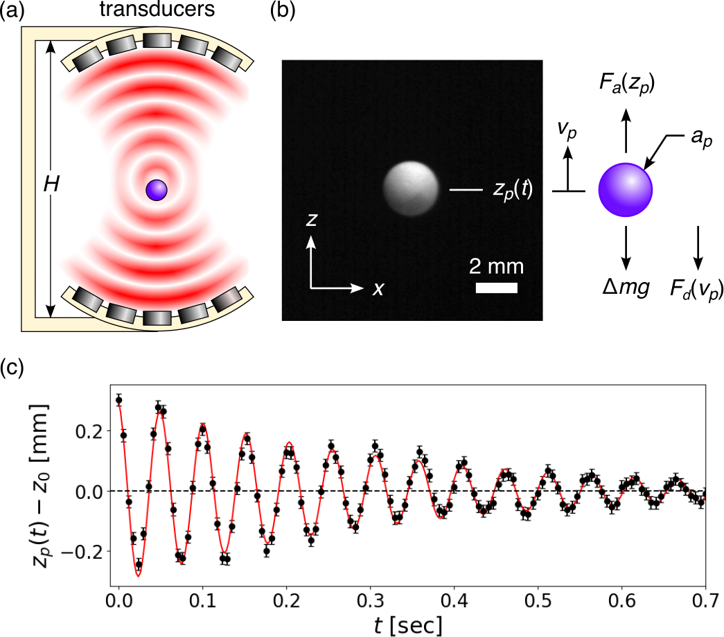
Figure 1: (a) Schematic diagram of the reference acoustic trap. (b) Typical video frame of a millimeter-scale styrofoam sphere levitated in the acoustic trap together with a schematic diagram of the forces acting on the particle. (c) Measured trajectory (black symbols) of a styrofoam bead returning to mechanical equilibrium in an acoustic trap compared with predictions of the damped oscillator model (red curve).

II Dynamics of an Acoustically Trapped Particle

II.1 Imaging measurements of damped oscillations

Figure 1(a) schematically represents the acoustic trapping system used for this study. Based on the standard TinyLev design [10], this acoustic levitator consists of two banks of piezoelectric ultrasonic transducers (MA40S4S, Murata, Inc.) with a resonance frequency around $40\text{\,}\mathrm{kHz}$. Each bank of $36$ transducers is driven sinusoidally by a function generator (DS345, Stanford Research Systems) and projects a traveling wave into a spherical volume of air. Interference between the two waves creates an array of acoustic traps along the instrument’s vertical axis. Figure 1(b) presents a video image of a millimeter-scale sphere of expanded polystyrene localized in air within one of the acoustic traps. The camera (Blackfly S USB3, FLIR) records the particle’s motions at $170\text{\,}\mathrm{f}\mathrm{r}\mathrm{a}\mathrm{m}\mathrm{e}\mathrm{s}\mathrm{/}\mathrm{s}$. with an exposure time of $2\text{\,}\mathrm{ms}$ and an effective magnification of $61\text{\,}\mathrm{\SIUnitSymbolMicro}\mathrm{m}\mathrm{/}\mathrm{p}\mathrm{i}\mathrm{x}\mathrm{e}\mathrm{l}$. Under these imaging conditions, the height of the particle in the trap, $z_{p}(t)$, can be measured in the imaging plane to within $\epsilon_{z}=$10\text{\,}\mathrm{\SIUnitSymbolMicro m}$$ by fitting for the image’s least bounding circle [18]. This method has the advantage over light-scattering techniques [15] that it also yields an estimate for the particle’s radius, $a_{p}$. For the particle in Fig. 1(b), $a_{p}=$1.346\pm 0.007\text{\,}\mathrm{mm}$$.

The particle can be made to oscillate in its trap by rapidly displacing it from its equilibrium position. This can be accomplished by abruptly changing the amplitude, frequency or relative phase [14] of the signals driving the two banks of transducers. The discrete symbols in Fig. 1(c) show the trapped particle’s displacement from its equilibrium position, $z_{p}(t)-z_{0}$, after an abrupt change of drive amplitude causes a displacement of $\Delta z=$-0.31\pm 0.01\text{\,}\mathrm{mm}$$. The (red) curve is a fit to the standard result for a damped harmonic oscillator,

$$z_{p}(t)=z_{0}+\Delta z\,e^{-\frac{1}{2}\gamma t}\cos(\Omega t)$$ (1)

for the oscillation frequency, $\Omega=$122.1\pm 0.2\text{\,}\mathrm{rad}\text{\,}{\mathrm{s}}^{-1}$=$19.43\pm 0.03\text{\,}\mathrm{Hz}$$ and the damping rate $\gamma=$6.3\pm 0.3\text{\,}{\mathrm{s}}^{-1}$$, in addition to $\Delta z$ and the equilibrium position, $z_{0}$. Although this fit appears to be satisfactory, the estimated parameters must be interpreted with care.

To illustrate the challenge, consider the standard Stokes result,

$$\gamma_{0}=\frac{6\pi\eta_{m}\,a_{p}}{m_{0}},$$ (2)

for the drag rate experienced by a sphere of radius $a_{p}$ and mass $m_{0}$ as it moves through a fluid with dynamic viscosity $\eta_{m}$. Expanded polystyrene sphere has a density of roughly $\rho_{p}=$30\text{\,}\mathrm{kg}\text{\,}{\mathrm{m}}^{-3}$$ [19], so that

$$m_{0}=\frac{4}{3}\pi a_{p}^{3}\,\rho_{p}=$0.3\text{\,}\mathrm{mg}$.$$ (3)

The viscosity of air under standard conditions is $\eta_{m}=$(1.825\pm 0.005)\text{\times}{10}^{-5}\text{\,}\mathrm{Pa}\text{\,}\mathrm{s}$$ [20]. Equation (2) therefore predicts $\gamma_{0}=$1.4\text{\,}{\mathrm{s}}^{-1}$$, which is a factor of four smaller than the measured value. Previous studies on similar systems have reported comparably large discrepancies between predicted and observed drag rates [15], and have addressed them phenomenologically with nonlinear drag models [12, 21, 15], if at all [13, 14].

Here, we demonstrate that the linear drag model underlying Eq. (1) indeed is appropriate for analyzing the oscillations of acoustically trapped objects provided that the parameters are suitably modified to account for the inertia of the displaced fluid [16, 17]. The enhanced model provides a basis for precisely measuring the density and mass of trapped objects without requiring the acoustic trap to be independently calibrated. The same approach can be used to calibrate the trap’s stiffness while accounting naturally for the influence of external forces such as gravity.

II.2 Acoustic forces

The force landscape experienced by an acoustically trapped object is dictated by the structure of the sound field. The counterpropagating waves in our instrument interfere to create a standing pressure wave along the central axis whose spatial dependence is approximately sinusoidal,

$$p(z)=2p_{0}\sin(kz),$$ (4)

near the midplane at $z=0$. Here, $p_{0}$ is the pressure amplitude due to a single bank of transducers and $k=\omega/c_{m}$ is the wave number of sound at frequency $\omega$ in a medium whose speed of sound is $c_{m}$. For acoustic levitation in air, $c_{m}=$343.5\pm 0.5\text{\,}\mathrm{m}\text{\,}{\mathrm{s}}^{-1}$$ under standard conditions [20].

The time-averaged acoustic force experienced by an object at height $z_{p}$ in the standing wave has the form [8, 9]

$$F_{a}(z_{p})=F_{0}\sin(2kz_{p}),$$ (5)

with an overall scale,

$$F_{0}=\chi\,kp_{0}^{2},$$ (6)

that depends on the frequency and amplitude of the sound wave, and on properties of the object and the medium through $\chi$. For a small spherical particle ($ka_{p}<1$), the acoustic response function is [8, 9]

$$\chi=\frac{4}{3}\pi a_{p}^{3}\,\kappa_{m}\left(1-\frac{\kappa_{p}}{\kappa_{m}}+3\frac{\rho_{p}-\rho_{m}}{2\rho_{p}+\rho_{m}}\right),$$ (7)

where $\rho_{p}$ and $\rho_{m}$ are the densities of the particle and medium, respectively, and $\kappa_{p}$ and $\kappa_{m}$ are their respective isentropic compressibilities. Dense incompressible particles have $\chi>0$ and therefore tend to be trapped at nodes of the pressure field.

External forces can displace the particle from the center of the acoustic trap, as depicted in Fig. 1(b). Gravity, in particular, acts on the particle’s buoyant mass,

$$\Delta m=m_{0}\left(1-\frac{\rho_{m}}{\rho_{p}}\right).$$ (8)

and displaces it from the pressure node at $z=0$ into mechanical equilibrium at

$$z_{0}=-\frac{1}{2k}\sin^{-1}\left(\frac{\Delta mg}{F_{0}}\right),$$ (9)

where $g=$9.81\text{\,}\mathrm{m}\text{\,}{\mathrm{s}}^{-2}$$ is the acceleration due to gravity.

As long as the particle does not move too far from the nodal plane, the acoustic trap exerts an approximately Hookean restoring force on the particle,

$$F_{a}(z_{p})\approx-\kappa\,(z_{p}-z_{0}),$$ (10)

with a stiffness,

$$\kappa=2kF_{0}\,\cos(2kz_{0}),$$ (11)

that depends on properties of the sound wave, properties of the particle and the strength of the external force. Calibrating the trap generally involves determining $\kappa$. Equation (11) clarifies that the trap cannot be calibrated with a reference object, as has been proposed [14], but instead requires a separate calibration for every set of experimental conditions.

II.3 Inertial corrections

An object moving in the trap’s potential energy well displaces the surrounding fluid medium and therefore experiences viscous drag. The standard Stokes result from Eq. (2) neglects the inertia of the fluid. For the special case of a sphere undergoing harmonic oscillations, inertial effects can be incorporated into a linear drag model,

$$F_{d}(v_{p})=-m(\Omega)\,\gamma(\Omega)\,v_{p},$$ (12)

by defining a dynamical mass

$$m(\Omega)=m_{0}\left(1+\frac{1}{2}\frac{\rho_{m}}{\rho_{p}}\left[1+\frac{9}{2}\frac{\delta(\Omega)}{a_{p}}\right]\right)$$ (13)

and a renormalized drag rate,

$$\gamma(\Omega)=\frac{6\pi\eta_{m}a_{p}}{m(\Omega)}\left(1+\frac{a_{p}}{\delta(\Omega)}\right)$$ (14)

that both depend on the oscillation frequency, $\Omega$, through the thickness of a boundary layer surrounding the sphere [16, 17],

$$\delta(\Omega)=\sqrt{\frac{2\eta_{m}}{\rho_{m}}\frac{1}{\Omega}}.$$ (15)

The inertia-corrected equation of motion for an acoustically levitated sphere is then analogous to the standard equation of motion for the damped harmonic oscillator,

$$\ddot{z}_{p}+\gamma(\Omega)\,\dot{z}_{p}+\Omega_{0}^{2}\,(z_{p}-z_{0})=0,$$ (16)

with a natural frequency,

$$\Omega_{0}(\Omega)=\sqrt{\frac{\kappa}{m(\Omega)}},$$ (17)

that is related to the measured frequency by

$$\Omega_{0}^{2}(\Omega)=\Omega^{2}+\frac{1}{4}\gamma^{2}(\Omega).$$ (18)

Unlike the standard harmonic oscillator, whose drag and restoring forces are independent of frequency, the natural frequency of an acoustically trapped object must be found by solving Eq. (18) self-consistently.

The derivation of Eq. (16) from boundary-layer theory establishes that Eq. (1) suitably models the dynamics of an object oscillating in an acoustic trap. Unlike dynamical models with nonlinear drag [12, 15], the damping rate predicted by Eq. (14) does not depend on the amplitude of the motion. This is consistent with the observation in Fig. 1(c) that a single constant value for $\gamma$ successfully accounts for viscous damping over the oscillating particle’s entire trajectory.

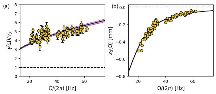
Figure 2: (a) Frequency dependence of the damping rate $\gamma(\Omega)$, Plot symbols present results from fits to measured trajectories, such as the example in Fig. 1(c). The solid curve is a fit to the boundary-layer model in Eq. (14) that yields $\rho_{p}=$28.9\pm 0.3\text{\,}\mathrm{kg}\text{\,}{\mathrm{m}}^{-3}$$. The horizontal dashed line reflects the standard Stokes result, $\gamma_{0}=$1.50\pm 0.03\text{\,}{\mathrm{s}}^{-1}$$. (b) Correlation of the axial offset, $z_{0}$, with the observed oscillation frequency, $\Omega$. The horizontal dashed line represents the nodal plane of the acoustic trap.

III Acoustodynamic Mass Determination

Measurements of $\gamma(\Omega)$ can be interpreted with Eq. (14) to estimate the mass density of the particle. The discrete points in Fig. 2(a) are measured by fitting recorded trajectories of the expanded polystyrene bead in Fig. 1. Different oscillation frequencies are obtained by adjusting the the amplitude, $V_{0}$, of the sinusoidal voltage powering the trap. It is not necessary to know how the trap strength, $F_{0}$, depends on $V_{0}$ to perform this measurement because $\gamma$ and $\Omega$ are both obtained directly from each measured trajectory. Taking the density of air to be $\rho_{m}=$1.220\pm 0.005\text{\,}\mathrm{kg}\text{\,}{\mathrm{m}}^{-3}$$ [20] leaves the particle’s density, $\rho_{p}$, as the only undetermined parameter in the model. The solid curve in Fig. 2(a) is a fit to Eq. (14) that yields $\rho_{p}=$28.9\pm 0.3\text{\,}\mathrm{kg}\text{\,}{\mathrm{m}}^{-3}$$, which is consistent with expectations for expanded polystyrene beads [19]. Inertial corrections quite convincingly account for the previously unexplained enhancement of the oscillating particle’s drag rate. In so doing, they also provide the basis for a precise and robust way to measure the mass density of millimeter-scale objects. Combining $\rho_{p}$ with the optically-measured radius yields the levitated object’s mass, $m_{0}=$0.31\pm 0.01\text{\,}\mathrm{mg}$$. Repeating this measurement on $10$ different beads from the same batch yields an average density of $\rho_{p}=$30.5\pm 0.2\text{\,}\mathrm{kg}\text{\,}{\mathrm{m}}^{-3}$$ and an average mass of $m_{0}=$0.295\pm 0.003\text{\,}\mathrm{mg}$$.

The precision of acoustodynamic mass determination is limited by run-to-run variability in the measured values of $\gamma(\Omega)$, which in turn can be ascribed to spurious transverse motions of the particle in its trap and to environmental factors such as vibrations and drafts. Even with these practical limitations, the $3\text{\,}\mathrm{\SIUnitSymbolMicro g}$ precision achieved in this representative realization is comparable to the performance of a conventional ultra-micro balance.

Previous acoustic trapping studies have attempted to measure the masses of levitated objects by interpreting their static displacements [22] with Eq. (9) or by interpreting their oscillation frequencies directly [14] without inertial corrections. Like conventional scales and balances, these approaches rely on independent calibration of the trap’s stiffness, $\kappa$. The present acoustodynamic approach avoids the need for such calibrations by comparing two independent time scales represented by $\Omega$ and $\gamma$, rather than two independent force scales.

Increasing the acoustic trap’s strength increases the oscillation frequency and lifts the particle toward the trap’s center. This correlation is reflected in the dependence of $z_{0}$ on $\Omega$ that is plotted in Fig. 2(b). These measurements can be interpreted within the boundary-layer model by combining Eq. (9) with Eq. (11) to obtain

$$z_{0}(\Omega)=-\frac{1}{2k}\,{\tan^{-1}}{\left(\frac{2kg}{\Omega_{0}^{2}(\Omega)}\frac{\Delta m}{m(\Omega)}\right)}+z_{\text{trap}},$$ (19)

where $z_{\text{trap}}$ is the height of the trap’s nodal plane in the camera’s field of view. The solid curve in Fig. 2(b) shows this model’s prediction using the value of $\rho_{p}$ obtained from $\gamma(\Omega)$. The data in Fig. 2(b) have been offset so that $z_{\text{trap}}=$0\pm 1.\text{\,}\mathrm{\SIUnitSymbolMicro m}$$. The excellent agreement between measurement and theory in this comparison serves to validate the acoustodynamically determined values of $\rho_{p}$ and $a_{p}$. Accurately identifying $z_{\text{trap}}$ also is valuable for force-extension measurements once the trap’s stiffness is calibrated.

IV Dynamic Trap Calibration

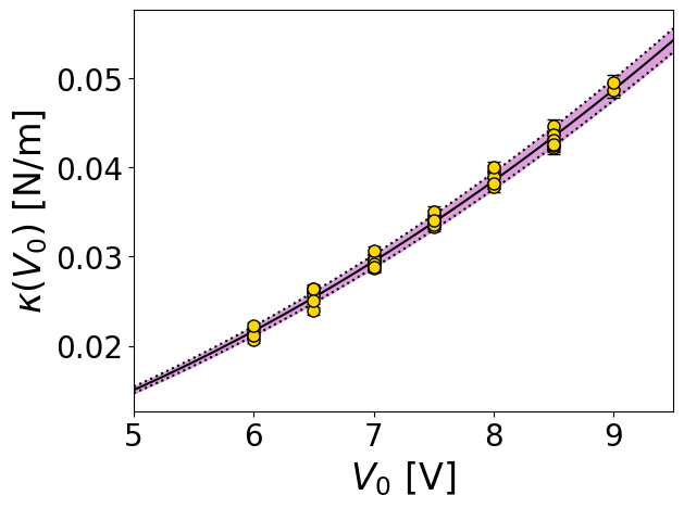
Figure 3: Dependence of the measured trap stiffness, $\kappa$, on the peak-to-peak voltage, $V_{0}$, used to power the acoustic trap’s transducer banks. The solid curve is a fit to Eq. (20b) for the calibration constant, $\alpha$.

The trap’s stiffness at each value of $V_{0}$ can be inferred from the particle’s damped oscillations through

$$\kappa(\Omega)=m(\Omega)\,\Omega_{0}^{2}(\Omega).$$ (20a)

Assuming that the pressure amplitude, $$p_{0} V_{0}$$, is proportional to the driving voltage, , Eq. (6) and Eq. (11) lead to an independent expression,

$$\kappa(V_{0})\approx\alpha V_{0}^{2}\ \left[1-\frac{1}{2}\left(\frac{k\Delta mg}{\alpha V_{0}^{2}}\right)^{2}\right],$$ (20b)

that can be compared with measurements based on Eq (20a) to obtain $\alpha$, the required calibration constant for this specific particle in the levitator. This result is valid when the particle is stably trapped against gravity, $F_{0}>\Delta mg$. Figure 3 shows the calibration obtained from the data set in Fig. 2 and yields $\alpha=$(6.02\pm 0.15)\text{\times}{10}^{-4}\text{\,}\mathrm{N}\text{\,}{\mathrm{m}}^{-1}\text{\,}{\mathrm{V}}^{-2}$$. Ignoring inertial corrections by using $m_{0}$ in Eq. (20a) would have yielded a significant underestimate for the calibration constant, $\alpha_{0}=$(5.77\pm 0.14)\text{\times}{10}^{-4}\text{\,}\mathrm{N}\text{\,}{\mathrm{m}}^{-1}\text{\,}{\mathrm{V}}^{-2}$$. Adding to the challenge, $m_{0}$ generally would not be known accurately for a millimeter-scale object a priori. The analytical framework described here solves this problem by providing self-consistent measurements of $\rho_{p}$, $m_{0}$ and $m(\Omega)$. The resulting calibration constant, $\alpha$, therefore should yield reliable results for the trap stiffness, $\kappa$.

V Discussion

Abruptly changing the trapping characteristics of an acoustic levitator sets a trapped object into a free oscillation that is damped by viscous drag in the surrounding medium. The resulting trajectory can be described with the standard model for a damped harmonic oscillator provided that inertial effects in the displaced fluid are taken into account self-consistently with hydrodynamic boundary-layer theory [16, 17]. These inertial corrections quantitatively resolve the large discrepancy between the measured drag rate and the Stokes prediction that has been noted in previous studies, but previously has been unexplained. The boundary-layer model is applicable for particle speeds substantially smaller than the speed of sound and Reynolds numbers well below the threshold for turbulence. For the present study, $v_{p}<$0.25\text{\,}\mathrm{m}\text{\,}{\mathrm{s}}^{-1}$$ and $\text{Re}=\rho_{p}a_{p}v_{p}/\eta_{m}\lesssim$23$$, so that both conditions are satisfied. The observation that $\text{Re}>1$ explains why the standard Stokes result substantially underestimates the drag rate.

Fitting measured trajectories to predictions of the boundary-layer model yields precise estimates for the trapped particle’s mass density and mass. Dynamic acoustic trapping therefore can be used to weigh millimeter-scale objects without requiring direct contact, including sub-milligram objects that can be challenging to weigh individually [23, 24, 25]. Generalizing this approach to accommodate aspherical objects, powders and fluids will be addressed in future studies.

Using the acoustic force field itself to set an object into oscillation provides a simple and effective method to calibrate the stiffness of an acoustic trap. This approach does not require the external intervention used in complementary calibration techniques, such as mechanically moving the sample relative to the levitator [26, 27]. The techniques discussed in this work therefore should facilitate fundamental research on the dynamics of granular materials in acoustic force landscapes.

Acoustodynamic mass determination should have near-term applications in the pharmaceutical industry for weighing individual pills and capsules, in the jewelry industry for weighing gemstones and precious metals, and in the nuclear power industry for massing individual fuel pellets. Many such applications currently rely on ultra-micro balances to cover the relevant mass range with good precision. Acoustodynamic mass determination offers several advantages. The measurement is inherently self-calibrated and is robust against environmental perturbations. Levitated samples never come in contact with surfaces, which is inherently beneficial for sensitive and hazardous materials, minimizes the likelihood of cross-contamination and simplifies integration with robotic sample handlers. Unlike conventional techniques, furthermore, acoustodynamic mass determination can operate freely in challenging environments such as microgravity.

References

- Kundt [1866] A. Kundt, On a new type of acoustic dust figure and on its application to determine the speed of sound in solid bodies and gases, Ann. Phys. 203, 497 (1866).
- Lim et al. [2019] M. X. Lim, A. Souslov, V. Vitelli, and H. M. Jaeger, Cluster formation by acoustic forces and active fluctuations in levitated granular matter, Nature Phys. 15, 460 (2019).
- Kline et al. [2020] A. G. Kline, M. X. Lim, and H. M. Jaeger, Precision measurement of tribocharging in acoustically levitated sub-millimeter grains, Rev. Sci. Instr. 91 (2020).
- Méndez Harper et al. [2022] J. Méndez Harper, D. Harvey, T. Huang, J. McGrath III, D. Meer, and J. C. Burton, The lifetime of charged dust in the atmosphere, PNAS nexus 1, pgac220 (2022).
- Lim and Jaeger [2023] M. X. Lim and H. M. Jaeger, Acoustically levitated lock and key grains, Phys. Rev. Res. 5, 013116 (2023).
- Foresti et al. [2013] D. Foresti, M. Nabavi, M. Klingauf, A. Ferrari, and D. Poulikakos, Acoustophoretic contactless transport and handling of matter in air, Proc. Natl. Acad. Sci. USA 110, 12549 (2013).
- Andrade et al. [2020] M. A. Andrade, A. Marzo, and J. C. Adamowski, Acoustic levitation in mid-air: Recent advances, challenges, and future perspectives, Appl. Phys. Lett. 116 (2020).
- Bruus [2012] H. Bruus, Acoustofluidics 2: Perturbation theory and ultrasound resonance modes, Lab Chip 12, 20 (2012).
- Abdelaziz and Grier [2020] M. A. Abdelaziz and D. G. Grier, Acoustokinetics: Crafting force landscapes from sound waves, Phys. Rev. Res. 2, 013172 (2020).
- Marzo et al. [2017] A. Marzo, A. Barnes, and B. W. Drinkwater, TinyLev: A multi-emitter single-axis acoustic levitator, Rev. Sci. Instr. 88, 085105 (2017).
- Marzo and Drinkwater [2019] A. Marzo and B. W. Drinkwater, Holographic acoustic tweezers, Proc. Natl. Acad. Sci. USA 116, 84 (2019).
- Pérez et al. [2014] N. Pérez, M. A. Andrade, R. Canetti, and J. C. Adamowski, Experimental determination of the dynamics of an acoustically levitated sphere, J. Appl. Phys. 116 (2014).
- Andrade et al. [2014] M. A. Andrade, N. Pérez, and J. C. Adamowski, Experimental study of the oscillation of spheres in an acoustic levitator, J. Acoust. Soc. Am. 136, 1518 (2014).
- Nakahara and Smith [2022] J. Nakahara and J. R. Smith, Acoustic balance: Weighing in ultrasonic non-contact manipulators, IEEE Robot. Autom. Lett. 7, 9145 (2022).
- Marrara et al. [2023] S. Marrara, D. B. Ciriza, A. Magazzù, R. Caruso, G. Lupò, R. Saija, A. Foti, P. G. Gucciardi, A. Mandanici, O. M. Maragò, et al., Optical calibration of holographic acoustic tweezers, IEEE Trans. Instrum. Meas. 72, 9600808 (2023).
- Landau and Lifshitz [1987] L. D. Landau and E. M. Lifshitz, Fluid Mechanics (Elsevier, 1987).
- Settnes and Bruus [2012] M. Settnes and H. Bruus, Forces acting on a small particle in an acoustical field in a viscous fluid, Phys. Rev. E 85, 016327 (2012).
- Woods and Gonzalez [2008] R. E. Woods and R. C. Gonzalez, Digital Image Processing (Pearson Education Ltd., 2008).
- Horvath [1994] J. Horvath, Expanded polystyrene (EPS) geofoam: an introduction to material behavior, Geotext. Geomembr. 13, 263 (1994).
- Lide [2017] D. Lide, ed., CRC Handbook of Chemistry and Physics, 104th ed. (Taylor & Francis, 2017).
- Fushimi et al. [2018] T. Fushimi, T. Hill, A. Marzo, and B. Drinkwater, Nonlinear trapping stiffness of mid-air single-axis acoustic levitators, Appl. Phys. Lett. 113 (2018).
- Trinh and Hsu [1986] E. Trinh and C. Hsu, Acoustic levitation methods for density measurements, J. Acoust. Soc. Am. 80, 1757 (1986).
- Shaw et al. [2016] G. A. Shaw, J. Stirling, J. A. Kramar, A. Moses, P. Abbott, R. Steiner, A. Koffman, J. R. Pratt, and Z. J. Kubarych, Milligram mass metrology using an electrostatic force balance, Metrologia 53, A86 (2016).
- Shaw [2018] G. A. Shaw, Current state of the art in small mass and force metrology within the International System of Units, Meas. Sci. Technol. 29, 072001 (2018).
- Ota et al. [2021] Y. Ota, M. Ueki, and N. Kuramoto, Evaluation of an automated mass comparator performance for mass calibration of sub-milligram weights, Measurement 172, 108841 (2021).
- Li et al. [2013] Y. Li, C. Lee, K. Ho Lam, and K. Kirk Shung, A simple method for evaluating the trapping performance of acoustic tweezers, Appl. Phys. Lett. 102, 084102 (2013).
- Lim et al. [2018] H. G. Lim, H. H. Kim, and C. Yoon, Evaluation method for acoustic trapping performance by tracking motion of trapped microparticle, Jpn. J. Appl. Phys. 57, 057202 (2018).