Computing the noncommutative inner rank by means of operator-valued free probability theory

Abstract.

We address the noncommutative version of the Edmonds’ problem, which asks to determine the inner rank of a matrix in noncommuting variables. We provide an algorithm for the calculation of this inner rank by relating the problem with the distribution of a basic object in free probability theory, namely operator-valued semicircular elements. We have to solve a matrix-valued quadratic equation, for which we provide precise analytical and numerical control on the fixed point algorithm for solving the equation. Numerical examples show the efficiency of the algorithm.

1. Introduction

We will address the question how to compute the rank of matrices in noncommuting variables. The classical, commuting, version of this is usually called the Edmonds’ problem: given a square matrix, where the entries are linear functions in commuting variables, one should decide whether this matrix is invertible over the field of rational functions; more general, one should calculate the rank of the matrix over the field of rational functions.

What we will consider here is a noncommutative version of this, where commuting variables are replaced by noncommuting ones; the usual rational functions are replaced by noncommutative rational functions (aka free skew field); and the commutative rank is replaced by the inner rank. The free skew field is a quite complicated object; there is no need for us to delve deeper into its theory, as we can and will state the problem in terms of the rank – for this we just have to deal with polynomials instead of rational functions. (Note however, that this relies on the non-trivial fact that the inner rank of our matrix over noncommutative polynomials is the same as its inner rank over noncommutative rational functions – a fact which is actually not true in the commutative setting!)

This noncommutative rank problem has become quite prominent in recent years and goes often under the name of noncommutative Edmonds’ problem. More precisely, let us consider a matrix $A=a_{1}\otimes\mathbf{x}_{1}+\ldots+a_{n}\otimes\mathbf{x}_{n}$, where $\mathbf{x}_{1},\dots,\mathbf{x}_{n}$ are noncommuting variables and $a_{1},\dots,a_{n}\in M_{N}(\mathbb{C})$ are arbitrary matrices of the same size $N$; $N$ is arbitrary and we want to treat all sizes simultaneously. The noncommutative Edmonds’ problem asks now whether $A$ is invertible over the noncommutative rational functions in $\mathbf{x}_{1},\dots,\mathbf{x}_{n}$; as pointed out above this is equivalent to asking whether $A$ is full, i.e., its noncommutative rank is equal to $N$. The noncommutative rank is here the inner rank $\operatorname{rank}(A)$, i.e., the smallest $r$ such that we can write $A$ as a product of an $N\times r$ and an $r\times N$-matrix. One can restrict to affine linear functions (i.e., constants plus linear functions) for the entries of those matrices. This fullness of the inner rank can also be equivalently decided by a more analytic object: to the matrix $A$ from above we associate a completely positive map $\eta:M_{N}(\mathbb{C})\to M_{N}(\mathbb{C})$, which is defined by $\eta(b):=\sum_{i=1}^{n}a_{i}ba_{i}^{*}$. In terms of $\eta$, the fullness condition for $A$ is equivalent to the fact that $\eta$ is rank-decreasing (here we have of course the ordinary commutative rank on the complex $N\times N$-matrices).

As shown in [9, 10], the noncommutative Edmonds’ problem has a deterministic polynomial time algorithm, via Gurvits’ noncommutative version of the Sinkhorn algorithm in order to certify whether $\eta$ is rank-decreasing. We will provide here another analytic approach to decide about the fullness of $A$, actually to calculate more generally the inner rank of $A$. We will also put some efforts into controlling the effectiveness and implementability of this analytic approach.

Since for arbitrary $A$ the inner rank of the $N\times N$-matrix $A$ is twice the inner rank of the selfadjoint $2N\times 2N$-matrix $\begin{pmatrix}0&A\\ A^{*}&0\end{pmatrix}$, it suffices to consider in the following selfadjoint $A$. For such a situation we will – instead of trying to find rectangular factorizations of $A$ or checking properties of the map $\eta$ – associate to $\eta$ (and thus to $A$) an $M_{N}(\mathbb{C})$-valued equation of the form

(1.1) $$zG(z)=\mathbf{1}+\eta(G(z))G(z);$$

for each $z\in\mathbb{C}^{+}$ there is exactly one solution $G(z)$ in the complex upper half-plane of $M_{N}(\mathbb{C})$, and if we take the normalized trace of this,

$$g(z):=\frac{1}{N}\operatorname{Tr}(G(z)),$$

then this $g(z)$ is the Cauchy transform of a uniquely determined probability measure $\mu_{A}$ on $\mathbb{R}$, i.e.,

$$g(z)=\int_{\mathbb{R}}\frac{1}{z-t}d\mu_{A}(t).$$

The inner rank of $A$ is now related to the mass of an atom of $\mu_{A}$ at zero; more precisely,

$$\operatorname{rank}(A)=N(1-\mu_{A}(\{0\})).$$

All those statements are non-trivial and follow from works in the last decade or so on free probability and in particular on analytic realizations of non-commutative formal variables via free semicircular random variables; a precise formulation for this connection will be given in Theorem 3.4. For general information on free probability we refer to [27, 18]; various numerical aspects of free probability were especially treated in [8, 22, 20].

The original problem of calculating the inner rank of our matrix $A$ can be stated as solving a system of quadratic equations, and the matrix equation (1.1) above is also not more than a system of quadratic equations for the entries of $G$. So one might wonder what advantage it brings to trade in one system of quadratic equations for another one. The point is that our system (1.1) has a lot of structure, especially positivity in the background (where, of course, $A=A^{*}$ is relevant), coming from the free probability interpretation of this setting, and thus we have in particular analytically controllable fixed point iterations to solve those systems. On the other hand, the general system for deciding on rectangular factorizations (even for selfadjoint $A$) is quite unstructured. It can be treated with general Groebner basis calculations, but their running time complexity makes this approach infeasible even for relatively small $N$.

In order to make concrete use of this relation between the inner rank of $A$ and the size of the atom of $\mu_{A}$ at zero we need precise analytical and numerical control on the fixed point algorithm for solving the equation (1.1) and we also have to deal with the de-convolution problem of extracting information about atoms of a probability measure from the knowledge of its Cauchy transform on the imaginary axis. All this will be done in the following. We will also provide numerical examples to show the efficiency of our algorithm.

2. A brief introduction to operator-valued free probability theory

Free probability theory, both in the scalar- and the operator-valued case, uses the language of noncommutative probability theory. While many fundamental concepts can be discussed already in some purely algebraic framework, it is more appropriate for our purposes to work in the setting of $C^{\ast}$-probability spaces. Thus, we stick right from the beginning to this framework. For a comprehensive introduction to the subject of $C^{\ast}$-algebras, we refer for instance to [2, Chapter II] and the references listed therein; for the readers’ convenience, we recall the terminology used in the sequel.

By a $C^{\ast}$-algebra, we mean a (complex) Banach $\ast$-algebra $\mathcal{A}$ in which the identity $\|x^{\ast}x\|=\|x\|^{2}$ holds for all $x\in\mathcal{A}$; if $\mathcal{A}$ has a unit element $\mathbf{1}$, we call $\mathcal{A}$ a unital $C^{\ast}$-algebra. A continuous linear functional $\phi:\mathcal{A}\to\mathbb{C}$ which is positive (meaning that $\phi(x^{\ast}x)\geq 0$ holds for all $x\in\mathcal{A}$) and satisfies $\|\phi\|=1$ is called a state. According to the Gelfand-Naimark theorem (see [2, Corollary II.6.4.10]), every $C^{\ast}$-algebra $\mathcal{A}$ admits an isometric $\ast$-representation on some associated Hilbert space $(H,\langle\cdot,\cdot\rangle)$; hence $\mathcal{A}$ can be identified with a norm-closed $\ast$-subalgebra of $B(H)$. Each vector $\xi\in H$ of length $\|\xi\|=1$ induces then a state $\phi:\mathcal{A}\to\mathbb{C},x\mapsto\langle x\xi,\xi\rangle$; such prototypical states are called vector states.

2.1. The scalar-valued case

A $C^{\ast}$-probability space is a tuple $(\mathcal{A},\phi)$ consisting of a unital $C^{\ast}$-algebra $\mathcal{A}$ and some distinguished state $\phi:\mathcal{A}\to\mathbb{C}$ to which we shall refer as the expectation on $\mathcal{A}$; elements of $\mathcal{A}$ will be called noncommutative random variables.

Let $(\mathcal{A}_{i})_{i\in I}$ be a family of unital subalgebras of $\mathcal{A}$. We say that $(\mathcal{A}_{i})_{i\in I}$ are freely independent if $\phi(x_{1}\cdots x_{n})=0$ holds for every choice of a finite number $n\in\mathbb{N}$ of elements $x_{1},\dots,x_{n}$ with $x_{j}\in\mathcal{A}_{i_{j}}$ and $\phi(x_{j})=0$ for $j=1,\dots,n$, where $i_{1},\dots,i_{n}\in I$ are indices satisfying $i_{1}\neq i_{2}\neq\ldots\neq i_{n}$. A family $(x_{i})_{i\in I}$ of noncommutative random variables in $\mathcal{A}$ is said to be freely independent if the unital subalgebras generated by the $x_{i}$’s are freely independent in the aforementioned sense.

To any selfadjoint noncommutative random variable $x\in\mathcal{A}$, we associate the Borel probability measure $\mu_{x}$ on the real line $\mathbb{R}$ which is uniquely determined by the requirement that $\mu$ encodes the moments of $x$, i.e., that $\phi(x^{k})=\int_{\mathbb{R}}t^{k}\,d\mu(t)$ holds for all $k\in\mathbb{N}_{0}$; we call $\mu_{x}$ the analytic distribution of $x$.

Of particular interest are (standard) semicircular elements as they constitute the free counterpart of normally distributed random variables in classical probability theory; more precisely, those are selfadjoint noncommutative random variables $s\in\mathcal{A}$ whose analytic distribution is the semicircular distribution, i.e., we have $d\mu_{s}(t)=\frac{1}{2\pi}\sqrt{4-t^{2}}\mathbf{1}_{[-2,2]}(t)\,dt$.

An important tool for the study of analytic distributions are Cauchy transforms (also known under the name Stieltjes transforms, especially in random matrix theory, but there usually with a different sign convention); for any finite Borel measure $\mu$ on the real line $\mathbb{R}$, the Cauchy transform of $\mu$ is defined as the holomorphic function

$$G_{\mu}:\ \mathbb{C}^{+}\to\mathbb{C}^{-},\quad z\mapsto\int_{\mathbb{R}}\frac{1}{z-t}\,d\mu(t),$$

where $\mathbb{C}^{+}$ and $\mathbb{C}^{-}$ denote the upper- and lower complex half-plane, respectively, i.e., $\mathbb{C}^{\pm}:=\{z\in\mathbb{C}\mid\pm\operatorname{Im}(z)>0\}$. In the case of the analytic distribution $\mu_{x}$ of some $x=x^{\ast}\in\mathcal{A}$, we have $G_{\mu_{x}}(z)=\phi((z\mathbf{1}-x)^{-1})$ for all $z\in\mathbb{C}^{+}$; we shall write $G_{x}$ for $G_{\mu_{x}}$ and refer to it as the Cauchy transform of $x$.

2.2. The operator-valued case

The step from the scalar- to the operator-valued case is done, roughly speaking, by allowing an arbitrary unital $C^{\ast}$-algebra $\mathcal{B}$ of $\mathcal{A}$ which is unitally embedded in $\mathcal{A}$ to take over the role of the complex numbers. Formally, an operator-valued $C^{\ast}$-probability space is a triple $(\mathcal{A},\mathbb{E},\mathcal{B})$ consisting of a unital $C^{\ast}$-algebra $\mathcal{A}$, a $C^{\ast}$-subalgebra $\mathcal{B}$ of $\mathcal{A}$ containing the unit element $\mathbf{1}$ of $\mathcal{A}$, and a conditional expectation $\mathbb{E}:\mathcal{A}\to\mathcal{B}$; the latter means that $\mathbb{E}$ is positive (in the sense that $\mathbb{E}[x^{\ast}x]$ is a positive element in $\mathcal{B}$ for every $x\in\mathcal{A}$) and further satisfies $\mathbb{E}[b]=b$ for all $b\in\mathcal{B}$ and $\mathbb{E}[b_{1}xb_{2}]=b_{1}\mathbb{E}[x]b_{2}$ for each $x\in\mathcal{A}$ and all $b_{1},b_{2}\in\mathcal{B}$.

Also the notion of free independence admits a natural extension to the operator-valued setting. Let $(\mathcal{A}_{i})_{i\in I}$ be a family of unital subalgebras of $\mathcal{A}$ with $\mathcal{B}\subseteq\mathcal{A}_{i}$ for $i\in I$. We say that $(\mathcal{A}_{i})_{i\in I}$ are freely independent with amalgamation over $\mathcal{B}$ if $\mathbb{E}[x_{1}\cdots x_{n}]=0$ holds for every choice of a finite number $n\in\mathbb{N}$ of elements $x_{1},\dots,x_{n}$ with $x_{j}\in\mathcal{A}_{i_{j}}$ and $\mathbb{E}[x_{j}]=0$ for $j=1,\dots,n$, where $i_{1},\dots,i_{n}\in I$ are indices satisfying $i_{1}\neq i_{2}\neq\ldots\neq i_{n}$. A family $(x_{i})_{i\in I}$ of noncommutative random variables in $\mathcal{A}$ is said to be freely independent with amalgamation over $\mathcal{B}$ if the unital subalgebras generated by $\mathcal{B}$ and the $x_{i}$’s are freely independent in the aforementioned sense.

In contrast to the scalar-valued case where it was possible to capture the moments of a single selfadjoint noncommutative random variables by a Borel probability measure on $\mathbb{R}$, such a handy description fails in the generality of operator-valued $C^{\ast}$-probability spaces. Therefore, we take a more algebraic position. Let $\mathcal{B}\langle\mathbf{x}\rangle$ be the $\ast$-algebra freely generated by $\mathcal{B}$ and a formal selfadjoint variable $\mathbf{x}$. We shall refer to the $\mathcal{B}$-bimodule map $\mu_{x}:\mathcal{B}\langle\mathbf{x}\rangle\to\mathcal{B}$ determined by

$$\mu_{x}(\mathbf{x}b_{1}\mathbf{x}\cdots\mathbf{x}b_{k-1}\mathbf{x}):=\mathbb{E}[xb_{1}x\cdots xb_{k-1}x]$$

as the $\mathcal{B}$-valued noncommutative distribution of $x$.

Let $\eta:\mathcal{B}\to\mathcal{B}$ be completely positive, i.e., a linear map $\eta:\mathcal{B}\to\mathcal{B}$ for which each of its amplifications $\eta^{(n)}:M_{n}(\mathcal{B})\to M_{n}(\mathcal{B})$ for $n\in\mathbb{N}$ is positive, where $\eta^{(n)}$ is defined by $\eta^{(n)}(b)=(\eta(b_{ij}))_{i,j=1}^{n}$ for every $b=(b_{ij})_{i,j=1}^{n}$ in $M_{n}(\mathcal{B})$ and $M_{n}(\mathcal{B})$ denotes the unital $C^{\ast}$-algebra of all $n\times n$ matrices over $\mathcal{B}$. A selfadjoint noncommutative random variable $s$ in $(\mathcal{A},\mathbb{E},\mathcal{B})$ is called centered $\mathcal{B}$-valued semicircular element with covariance $\eta$ if

(2.1) $$\mu_{s}(\mathbf{x}b_{1}\mathbf{x}\cdots\mathbf{x}b_{k-1}\mathbf{x})=\sum_{\pi\in\operatorname{NC}_{2}(k)}\eta_{\pi}(b_{1},\dots,b_{k-1})$$

for all $k\in\mathbb{N}$ and $b_{1},\dots,b_{k-1}\in\mathcal{B}$, where $\operatorname{NC}_{2}(k)$ denotes the set of all non-crossing parings on $\{1,\dots,k\}$ and $\eta_{\pi}$ is given by applying $\eta$ to its arguments according to the block structure of $\pi\in\operatorname{NC}_{2}(k)$. More generally, a $\mathcal{B}$-valued semicircular element with covariance $\eta$ means a selfadjoint noncommutative random variable $s$ in $(\mathcal{A},\mathbb{E},\mathcal{B})$ for which its centered version $s^{\circ}:=s-\mathbb{E}[s]$ gives a centered $\mathcal{B}$-valued semicircular element with covariance $\eta$.

Notice that if $s$ is a (centered) $\mathcal{B}$-valued semicircular element in $(\mathcal{A},\mathbb{E},\mathcal{B})$ with covariance $\eta$, then in particular $\eta(b)=\mu_{s}(\mathbf{x}b\mathbf{x})=\mathbb{E}[sbs]$ for every $b\in\mathcal{B}$; as $\mathbb{E}$ is completely positive, the latter shows that it causes no loss of generality to require $\eta$ to be completely positive. In fact, for every completely positive map $\eta:\mathcal{B}\to\mathcal{B}$ on a unital $C^{\ast}$-algebra $\mathcal{B}$, there exists a $C^{\ast}$-probability space $(\mathcal{A},\mathbb{E},\mathcal{B})$ and a $\mathcal{B}$-valued semicircular element $s$ in $(\mathcal{A},\mathbb{E},\mathcal{B})$ such that $\eta(b)=\mathbb{E}[sbs]$ for all $b\in\mathcal{B}$. This follows from [21, Proposition 2.2] since the $\mathcal{B}$-valued distribution defined by (2.1) is exponentially bounded, as one easily verifies via its defining formula, and moreover positive, as explained in [24, Theorem 4.3.1]; for a discussion of this question in the von Neumann algebra case, we refer the interested reader to [23].

Cauchy transforms can also be generalized to the operator-valued realm where they provide an enormously useful analytic tool. For any selfadjoint noncommutative random variable $x\in\mathcal{A}$, we define the $\mathcal{B}$-valued Cauchy transform of $x$ by

$$G_{x}^{\mathcal{B}}:\ \mathbb{H}^{+}(\mathcal{B})\to\mathbb{H}^{-}(\mathcal{B}),\quad b\mapsto\mathbb{E}\big{[}(b-x)^{-1}\big{]},$$

where $\mathbb{H}^{+}(\mathcal{B})$ and $\mathbb{H}^{-}(\mathcal{B})$ are the upper and lower half-plane in $\mathcal{B}$, respectively, i.e., $\mathbb{H}^{\pm}(\mathcal{B}):=\{b\in\mathcal{B}\mid\exists\varepsilon>0:\pm\operatorname{Im}(b)\geq\varepsilon\mathbf{1}\}$ where we set $\operatorname{Im}(b):=\frac{1}{2i}(b-b^{\ast})$; notice that $b\in\mathcal{B}$ belongs to $\mathbb{H}^{\pm}(\mathcal{B})$ if and only if $\pm\operatorname{Im}(b)$ is an invertible positive element in $\mathcal{B}$. We recall that we have

(2.2) $$\|(b-x)^{-1}\|\leq\|\operatorname{Im}(b)^{-1}\|$$

and hence

(2.3) $$\|G_{x}^{\mathcal{B}}(b)\|\leq\|\operatorname{Im}(b)^{-1}\|$$

for all $b\in\mathbb{H}^{+}(\mathcal{B})$. Whenever the underlying $C^{\ast}$-algebra $\mathcal{B}$ is clear from the context, we will simply write $G_{x}$ instead of $G_{x}^{\mathcal{B}}$.

We know from [24, Theorem 4.1.12] that the $\mathcal{B}$-valued Cauchy transform $G_{s}:\mathbb{H}^{+}(\mathcal{B})\to\mathbb{H}^{-}(\mathcal{B})$ of a centered operator-valued semicircular element with covariance $\eta$ solves the equation

(2.4) $$bG_{s}(b)=\mathbf{1}+\eta(G_{s}(b))G_{s}(b)\qquad\text{for $b\in\mathbb{H}^{+}(\mathcal{B})$},$$

where $\mathbf{1}$ denotes the unit in $\mathcal{B}$. From [14], we further learn that this equation uniquely determines $G_{s}$ among all functions defined on $\mathbb{H}^{+}(\mathcal{B})$ and taking values in $\mathbb{H}^{-}(\mathcal{B})$.

In contrast to the scalar-valued case, $\mathcal{B}$-valued Cauchy transforms are in general not able to capture the $\mathcal{B}$-valued distribution of the selfadjoint noncommutative random variable they are associated with. To this end, Voiculescu [28] brought up the idea to consider their fully matricial extension, which we are going to explain next; see [4] for a detailed account of how one can recover the operator-valued distribution of a selfadjoint noncommutative random variable from the fully matricial extension of its associated operator-valued Cauchy transform. First, let us point out that to every operator-valued $C^{\ast}$-probability space $(\mathcal{A},\mathbb{E},\mathcal{B})$, we can associate for each $n\in\mathbb{N}$ the operator-valued $C^{\ast}$-probability space $(M_{n}(\mathcal{A}),\mathbb{E}^{(n)},M_{n}(\mathcal{B}))$. For every selfadjoint noncommutative random variable $x\in\mathcal{A}$, there is accordingly a whole family $(G^{(n)}_{x})_{n\in\mathbb{N}}$ of operator-valued Cauchy transforms naturally associated to it, namely

$$G^{(n)}_{x}:=G^{M_{n}(\mathcal{B})}_{x^{\oplus n}}:\ \mathbb{H}^{+}(M_{n}(\mathcal{B}))\to\mathbb{H}^{+}(M_{n}(\mathcal{B})),\quad b\mapsto\mathbb{E}^{(n)}\big{[}\big{(}b-x^{\oplus n}\big{)}^{-1}\big{]},$$

where $x^{\oplus n}\in M_{n}(\mathcal{A})$ is the matrix with $x$ along the diagonal and zeros in all its other entries. This family $(G^{(n)}_{x})_{n\in\mathbb{N}}$ defines a free noncommutative function in the sense of [15]; a characterization of those free noncommutative functions which arise as fully matricial extensions of the operator-valued Cauchy transforms of selfadjoint noncommutative random variables has been found in [29].

For a centered operator-valued semicircular element $s$ in $(\mathcal{A},\mathbb{E},\mathcal{B})$ with covariance $\eta:\mathcal{B}\to\mathcal{B}$, we know that $s^{\oplus n}$ is again a centered operator-valued semicircular element with covariance $\eta^{(n)}:M_{n}(\mathcal{B})\to M_{n}(\mathcal{B})$. By applying (2.4) in the setting of $(M_{n}(\mathcal{A}),\mathbb{E}^{(n)},M_{n}(\mathcal{B}))$ for $s^{\oplus n}$, we derive that $(G^{(n)}_{s})_{n\in\mathbb{N}}$ satisfies

(2.5) $$bG^{(n)}_{s}(b)=\mathbf{1}^{\oplus n}+\eta^{(n)}(G^{(n)}_{s}(b))G^{(n)}_{s}(b)\qquad\text{for $b\in\mathbb{H}^{+}(M_{n}(\mathcal{B}))$}.$$

3. Reading off the size of an atom at zero from Cauchy transforms

Let $\mu$ be a finite Borel measure on the real line $\mathbb{R}$. It is well-known that one can recover $\mu$ with the help of the Stieltjes inversion formula from its Cauchy transform $G_{\mu}$; more precisely, one has that the finite Borel measures $\mu_{\varepsilon}$ defined by $d\mu_{\varepsilon}(t):=-\frac{1}{\pi}\operatorname{Im}(G_{\mu}(t+i\varepsilon))\,dt$ converge weakly to $\mu$ as $\varepsilon\searrow 0$. Here, we aim at computing the value $\mu(\{0\})$ from the knowledge of (arbitrarily good approximations of) $G_{\mu}$; while we are mostly interested in the case of probability measures, we cover here the more general case of finite measures. To this end, we define the function

$$\theta_{\mu}:\ \mathbb{R}^{+}\to\mathbb{R}^{+},\quad y\mapsto-y\operatorname{Im}(G_{\mu}(iy))$$

on $\mathbb{R}^{+}:=(0,\infty)$. Note that $\theta_{\mu}(y)=\operatorname{Re}(iyG_{\mu}(iy))$ for all $y\in\mathbb{R}^{+}$.

Using the notation $\mathfrak{a}_{k}(\mu):=\int_{\mathbb{R}}|t|^{k}\,d\mu(t)$ for $k\in\mathbb{N}_{0}$, we start by collecting some properties of $\theta_{\mu}$:

Proposition 3.1.

Let $\mu$ be a Borel measure on the real line $\mathbb{R}$. Consider the associated Cauchy transform $G_{\mu}:\mathbb{C}^{+}\to\mathbb{C}^{-}$ and the function $\theta_{\mu}:\mathbb{R}^{+}\to\mathbb{R}^{+}$. Then, the following statements hold true:

1. We have $\lim_{y\to\infty}\theta_{\mu}(y)=\mu(\mathbb{R})$ and $\lim_{y\to 0}\theta_{\mu}(y)=\mu(\{0\})$.

2. For each $y\in\mathbb{R}^{+}$ we have that

   $$\theta_{\mu}(y)=\int_{\mathbb{R}}\frac{y^{2}}{y^{2}+t^{2}}\,d\mu(t)\quad\text{and}\quad\theta_{\mu}^{\prime}(y)=\int_{\mathbb{R}}\frac{2yt^{2}}{(y^{2}+t^{2})^{2}}\,d\mu(t).$$

   In particular, the function $\theta_{\mu}$ is increasing.

3. The function $\theta_{\mu}$ bounds $\mu(\{0\})$ from above, i.e., $\mu(\{0\})\leq\theta_{\mu}(y)$ for all $y\in\mathbb{R}^{+}$.

4. We have that $\theta_{\mu}^{\prime}(y)\leq\frac{\mu(\mathbb{R})}{2y}$ for all $y\in\mathbb{R}^{+}$.

5. If $\mu$ has finite moments of order $2(k+1)$ for some $k\geq 1$, then for all $y\in\mathbb{R}^{+}$

   $$\theta_{\mu}^{\prime}(y)\geq\frac{2\mathfrak{a}_{k}(\mu)^{2}y}{\mathfrak{a}_{2(k-1)}(\mu)y^{4}+2\mathfrak{a}_{2k}(\mu)y^{2}+\mathfrak{a}_{2(k+1)}(\mu)}.$$

Proof.

1. This follows from the well-known facts that $\lim_{\sphericalangle z\to\infty}zG_{\mu}(z)=1$ and $\lim_{\sphericalangle z\to 0}zG_{\mu}(z)=\mu(\{0\})$. Indeed, the latter implies that in particular $\lim_{y\to\infty}iyG_{\mu}(iy)=1$ and $\lim_{y\to 0}iyG_{\mu}(iy)=\mu(\{0\})$, which yields as desired $\lim_{y\to\infty}\theta_{\mu}(y)=1$ and $\lim_{y\to 0}\theta_{\mu}(y)=\mu(\{0\})$ since $\theta_{\mu}(y)=\operatorname{Re}(iyG_{\mu}(iy))$.

2. For each $y\in\mathbb{R}^{+}$, we have $G_{\mu}(iy)=\int_{\mathbb{R}}\frac{1}{iy-t}\,d\mu(t)$ and hence

   $$\operatorname{Im}(G_{\mu}(iy))=\int_{\mathbb{R}}\operatorname{Im}\Big{(}\frac{1}{iy-t}\Big{)}\,d\mu(t)=-\int_{\mathbb{R}}\frac{y}{y^{2}+t^{2}}\,d\mu(t).$$

   From this, we easily deduce the asserted integral representations of $\theta_{\mu}$ and $\theta_{\mu}^{\prime}$; the latter tells us that $\theta_{\mu}$ is increasing.

3. Follows from combining (i) and (ii).

4. By the inequality between the arithmetic and the geometric mean, we see that $\frac{2yt^{2}}{(y^{2}+t^{2})^{2}}\leq\frac{1}{2y}$ for each $y\in\mathbb{R}^{+}$ and all $t\in\mathbb{R}$. Thus, using the formula derived in (ii) and since $\mu$ is a probability measure, we conclude that $\theta_{\mu}^{\prime}(y)\leq\frac{\mu(\mathbb{R})}{2y}$ for all $y\in\mathbb{R}^{+}$ as desired.

5. For each $y\in\mathbb{R}^{+}$, the Cauchy-Schwarz inequality yields

   $$\sqrt{2y}\int_{\mathbb{R}}|t|^{k}\,d\mu(t) =\int_{\mathbb{R}}\frac{\sqrt{2y}|t|}{y^{2}+t^{2}}\,|t|^{k-1}(y^{2}+t^{2})\,d\mu(t)$$

   $$\leq\Big{(}\int_{\mathbb{R}}\frac{2yt^{2}}{(y^{2}+t^{2})^{2}}\,d\mu(t)\Big{)}^{1/2}\Big{(}\int_{\mathbb{R}}t^{2(k-1)}(y^{2}+t^{2})^{2}\,d\mu(t)\Big{)}^{1/2}.$$

   From the latter and (ii), we infer the bound stated in (v). ∎

Remarkably, Proposition 3.1 (v) yields a bound for the size of the atom of $\mu$ at $0$ which depends only on small (absolute) moments of $\mu$. The precise statement reads as follows.

Corollary 3.2.

In the situation of Proposition 3.1 (v), we have

$$\mu(\{0\})\leq\begin{cases}1-\frac{\mathfrak{a}_{k}(\mu)^{2}}{\mathfrak{a}_{2k}(\mu)}\,\rho\big{(}\frac{\pi}{2}-\arctan(\rho)\big{)}&\text{if $\mathfrak{a}_{2(k+1)}(\mu)\mathfrak{a}_{2(k-1)}(\mu)>\mathfrak{a}_{2k}(\mu)^{2}$}\\ 1-\frac{\mathfrak{a}_{k}(\mu)^{2}}{\mathfrak{a}_{2k}(\mu)}&\text{if $\mathfrak{a}_{2(k+1)}(\mu)\mathfrak{a}_{2(k-1)}(\mu)=\mathfrak{a}_{2k}(\mu)^{2}$}\end{cases},$$

where we abbreviate

$$\rho:=\bigg{(}\frac{\mathfrak{a}_{2(k+1)}(\mu)\mathfrak{a}_{2(k-1)}(\mu)}{\mathfrak{a}_{2k}(\mu)^{2}}-1\bigg{)}^{-\frac{1}{2}}.$$

Proof.

By the properties of the function $\theta_{\mu}$ summarized in Proposition 3.1, we have that

$$1-\mu(\{0\})=\int^{\infty}_{0}\theta_{\mu}^{\prime}(y)\,dy\geq\int^{\infty}_{0}\frac{2\mathfrak{a}_{k}(\mu)^{2}y}{\mathfrak{a}_{2(k-1)}(\mu)y^{4}+2\mathfrak{a}_{2k}(\mu)y^{2}+\mathfrak{a}_{2(k+1)}(\mu)}\,dy.$$

In order to evaluate the integral on the right, we use the following formula: for all $\alpha,\beta\in\mathbb{R}$ satisfying $\beta\geq\alpha^{2}$, we have

$$\int^{\infty}_{0}\frac{2y}{y^{4}+2\alpha y^{2}+\beta}\,dy =\int^{\infty}_{\alpha}\frac{1}{y^{2}+(\beta-\alpha^{2})}\,dy$$

$$=\begin{cases}\frac{1}{\sqrt{\beta-\alpha^{2}}}\Big{(}\frac{\pi}{2}-\arctan\big{(}\frac{\alpha}{\sqrt{\beta-\alpha^{2}}}\big{)}\Big{)}&\text{if $\beta>\alpha^{2}$}\\ \frac{1}{\alpha}&\text{if $\beta=\alpha^{2}$}\end{cases}.$$

Applying this for $\alpha=\frac{\mathfrak{a}_{2k}(\mu)}{\mathfrak{a}_{2(k-1)}(\mu)}$ and $\beta=\frac{\mathfrak{a}_{2(k+1)}(\mu)}{\mathfrak{a}_{2(k-1)}(\mu)}$ (which satisfy the condition $\beta\geq\alpha^{2}$ since $\mathfrak{a}_{2k}(\mu)^{2}\leq\mathfrak{a}_{2(k-1)}(\mu)\mathfrak{a}_{2(k+1)}(\mu)$ by the Cauchy-Schwarz inequality) and combining that result with the previously obtained bound for $1-\mu(\{0\})$, we conclude the proof. ∎

In Remark 3.6 below, we discuss Corollary 3.2 in the case of matrix-valued semicircular elements which are at the core of our investigations. In general, the estimates obtained in this way are much weaker than what can be achieved with the methods developed later in this paper, but still can lead to non-trivial results; see Example 3.7.

In the applications we are interested in, $\mu$ is a Borel probability measure and we have access to $\theta_{\mu}(y)$ at any point $y\in\mathbb{R}^{+}$; we want to use this information to compute $\mu(\{0\})$. We will work in such situations where the possible values of $\mu(\{0\})$ are limited to a discrete subset of the interval $[0,1]$; then, thanks to Proposition 3.1, once we found $y\in\mathbb{R}^{+}$ for which $\theta_{\mu}(y)$ falls below the smallest positive value that $\mu(\{0\})$ can attain, we can conclude that $\mu(\{0\})$ must be zero. For this approach, however, we lack some techniques to predict how small $y$ must be to decide reliably whether $\mu(\{0\})$ is zero or not and to find its precise value in the latter case. This problem is addressed in the following proposition for Borel probability measures $\mu$ of regular type, i.e., those which are of the form $\mu=\mu(\{0\})\delta_{0}+\nu$ for some Borel measure $\nu$ satisfying

(3.1) $$\nu([-r,r])\leq cr^{\beta}\qquad\text{for all $0<r<r_{0}$}$$

with some $c\geq 0$, $\beta\in(0,1]$ and $r_{0}>0$; note that we necessarily have $\nu(\mathbb{R})=1-\mu(\{0\})$. We emphasize that (3.1) allows $c=0$; thus, the class of Borel probability measures of regular type includes those Borel probability measures whose support is contained in $\mathbb{R}\setminus(-r_{0},r_{0})$ for some $r_{0}>0$ except, possibly, an atom at zero.

Proposition 3.3.

Let $\mu$ be a Borel probability measure on $\mathbb{R}$ which is of regular type such that (3.1) holds. Let $\gamma:=\frac{2}{2+\beta}$ and $y_{0}:=r_{0}^{1/\gamma}$, then

$$\theta_{\mu}(y)-\mu(\{0\})\leq(c+\nu(\mathbb{R}))y^{\frac{2\beta}{2+\beta}}\qquad\text{for all $0<y<y_{0}$}.$$

Proof.

First of all, we note that $G_{\mu}(z)=\mu(\{0\})\frac{1}{z}+G_{\nu}(z)$ for all $z\in\mathbb{C}^{+}$ and hence $\theta_{\mu}(y)=\mu(\{0\})+\theta_{\nu}(y)$ for all $y\in\mathbb{R}^{+}$.

Now for all $0<y<y_{0}$ we have $r:=y^{\gamma}<y_{0}^{\gamma}=r_{0}$, so we get

$$\int_{[-r,r]}\frac{y^{2}}{y^{2}+t^{2}}\,d\nu(t) \leq\nu([-r,r])\leq cr^{\beta}=cy^{\frac{2\beta}{2+\beta}},$$

$$\int_{\mathbb{R}\setminus[-r,r]}\frac{y^{2}}{y^{2}+t^{2}}\,d\nu(t) \leq\nu(\mathbb{R})\Big{(}\frac{y}{r}\Big{)}^{2}=\nu(\mathbb{R})y^{\frac{2\beta}{2+\beta}},$$

and hence, using Proposition 3.1 (ii), that $\theta_{\nu}(y)\leq(c+\nu(\mathbb{R}))y^{\frac{2\beta}{2+\beta}}$.

Combining both results, we obtain the asserted bound. ∎

In the next theorem, we summarize results from [25, 19] showing that Borel probability measures of regular type arise as analytic distributions of matrix-valued semicircular elements. This class of operators allows us to bridge the gap between the algebraic problem of determining the inner rank of linear matrix pencils over the ring of noncommutative polynomials and the analytic tools originating in free probability theory.

To this end, we need to work in the setting of tracial $W^{\ast}$-probability spaces. Therefore, we outline some basic facts about von Neumann algebras; fore more details, we refer to [26, 2], for instance. Let us recall that a von Neumann algebra $\mathcal{M}$ is a unital $\ast$-subalgebra of $B(H)$ which is closed with respect to the weak, or equivalently, with respect to the strong operator topology. Since these topologies are weaker than the topology induced by the norm $\|\cdot\|$ on $B(H)$, every von Neumann algebra $\mathcal{M}$ is in particular a unital $C^{\ast}$-algebra. We call $(\mathcal{M},\tau)$ a tracial $W^{\ast}$-probability space if $\mathcal{M}\subseteq B(H)$ is a von Neumann algebra and $\tau:\mathcal{M}\to\mathbb{C}$ a state, which is moreover normal (i.e., according to the characterization of normality given in [2, Theorem III.2.1.4], the restriction of $\tau$ to $\{x\in\mathcal{M}\mid\|x\|\leq 1\}$, the unit ball of $\mathcal{M}$, is continuous with respect to the weak, or equivalently, with respect to the strong operator topology), faithful (i.e., if $x\in\mathcal{M}$ is such that $\tau(x^{\ast}x)=0$, then $x=0$), and tracial (i.e., we have $\tau(xy)=\tau(yx)$ for all $x,y\in\mathcal{M}$).

Theorem 3.4.

Let $s_{1},\dots,s_{n}$ be freely independent standard semicircular elements in some tracial $W^{\ast}$-probability space $(\mathcal{M},\tau)$. Consider further some selfadjoint matrices $a_{1},\dots,a_{n}$ in $M_{N}(\mathbb{C})$. We define the operator

$$S=a_{1}\otimes s_{1}+\ldots+a_{n}\otimes s_{n}$$

which lives in the tracial $W^{\ast}$-probability space $(M_{N}(\mathbb{C})\otimes\mathcal{M},\operatorname{tr}_{N}\otimes\tau)$. Then the following statements hold true:

1. The analytic distribution $\mu_{S}$ of $S$ is of regular type.

2. The only possible values of $\mu_{S}(\{0\})$ are $\{\frac{k}{N}\mid k=0,1,\dots,N\}$.

3. The inner rank $\operatorname{rank}(A)$ of the linear pencil

   $$A:=a_{1}\otimes\mathbf{x}_{1}+\ldots+a_{n}\otimes\mathbf{x}_{n}$$

   over the ring $\mathbb{C}\langle\mathbf{x}_{1},\dots,\mathbf{x}_{n}\rangle$ of noncommutative polynomials in $n$ formal noncommuting variables $\mathbf{x}_{1},\dots,\mathbf{x}_{n}$ is given by

   $$\operatorname{rank}(A)=N\big{(}1-\mu_{S}(\{0\})\big{)}.$$

Before giving the proof of Theorem 3.4, we recall that the Novikov-Shubin invariant $\alpha(x)\in[0,\infty]\cup\{\infty^{+}\}$ of a positive operator $x$ in some tracial $W^{\ast}$-probability space $(\mathcal{M},\tau)$ is defined as

$$\alpha(x):=\liminf_{t\searrow 0}\frac{\log\big{(}\mu_{x}([0,t])-\mu_{x}(\{0\})\big{)}}{\log(t)}\in[0,\infty]$$

if $\mu_{x}([0,t])>\mu_{x}(\{0\})$ is satisfied for all $t>0$ and as $\alpha(x):=\infty^{+}$ otherwise. We emphasize that $\infty^{+}$ is nothing but a (reasonable) notation which is used to distinguish the case of an isolated atom at $0$.

Proof.

1. It follows from [25, Theorem 5.4] that the Cauchy transform of $\mu_{S^{2}}$, the analytic distribution of the positive operator $S^{2}$, is algebraic. Hence, [25, Lemma 5.14] yields that the Novikov-Shubin invariant $\alpha(S^{2})$ of $S^{2}$ is either a non-zero rational number or $\infty^{+}$.

   Let us consider the case $\alpha(S^{2})=\infty^{+}$ first. Then $0$ is an isolated point of the spectrum of $S^{2}$. Using spectral mapping, we infer that $0$ is also an isolated point in the spectrum of $S$. Thus, $\mu_{S}$ decomposes as $\mu_{S}=\mu_{S}(\{0\})\delta_{0}+\nu$, where $\nu$ is supported on $\mathbb{R}\setminus(-r_{0},r_{0})$ for some $r_{0}>0$ and we conclude that $\mu_{S}$ is of regular type.

   Now, we consider the case $\alpha(S^{2})\in\mathbb{Q}\cap(0,\infty)$. Choose any $0<\alpha<\alpha(S^{2})$. From the definition of $\alpha(S^{2})$, we infer that $\mu_{S^{2}}$ satisfies $\mu_{S^{2}}((0,t])=\mu_{S^{2}}([0,t])-\mu_{S^{2}}(\{0\})\leq t^{\alpha}$ for sufficiently small $t$, say for $0<t<t_{0}$. Since $\mu_{S}([-r,r])=\mu_{S^{2}}([0,r^{2}])$ and $\mu_{S}(\{0\})=\mu_{S^{2}}(\{0\})$, we infer that $\mu_{S}$ satisfies $\mu_{S}([-r,r])-\mu_{S}(\{0\})\leq r^{2\alpha}$ for all $0<r<r_{0}$ with $r_{0}:=t_{0}^{1/2}$. If we set $\nu:=\mu_{S}-\mu_{S}(\{0\})\delta_{0}$, then $\nu([-r,r])\leq r^{\beta}$ for all $0<r<r_{0}$ with $\beta:=2\alpha$; thus, $\mu_{S}$ again is of regular type.

2. This follows by an application of Theorem 1.1 (2) in [25].

3. The formula for the inner rank can be deduced from Theorem 5.21 in [19]; see also Remark 3.5 below.∎

Remark 3.5.

From [19], we learn that the conclusion of Theorem 3.4 (iii) is not at all limited to $n$-tuples of freely independent standard semicircular elements. Actually, we may replace $(s_{1},\dots,s_{n})$ by any $n$-tuple $(x_{1},\dots,x_{n})$ of selfadjoint operators in a tracial $W^{\ast}$-probability space $(\mathcal{M},\tau)$ which satisfy the condition $\Delta(x_{1},\dots,x_{n})=n$, where $\Delta(x_{1},\dots,x_{n})$ is the quantity introduced by Connes and Shlyakhtenko in [6, Section 3.1.2]. For any such $n$-tuple $(x_{1},\dots,x_{n})$, [19, Theorem 5.21] yields that

$$\operatorname{rank}(A)=N\big{(}1-\mu_{X}(\{0\})\big{)},$$

where $A=a_{1}\otimes\mathbf{x}_{1}+\ldots+a_{n}\otimes\mathbf{x}_{n}$ is a linear pencil over $\mathbb{C}\langle\mathbf{x}_{1},\dots,\mathbf{x}_{n}\rangle$ with selfadjoint coefficients $a_{1},\dots,a_{n}\in M_{N}(\mathbb{C})$ and $X:=A(x_{1},\dots,x_{n})$ is a selfadjoint noncommutative random variable in $(M_{N}(\mathbb{C})\otimes\mathcal{M},\operatorname{tr}_{N}\otimes\tau)$. For the sake of completeness, though this is not relevant for our purpose, we stress that even the restriction to linear pencils is not necessary as the result remains true for all selfadjoint $A\in M_{N}(\mathbb{C})\otimes\mathbb{C}\langle\mathbf{x}_{1},\dots,\mathbf{x}_{n}\rangle$; see [19, Corollary 5.15].

Remark 3.6.

In the light of Theorem 3.4, we now return to Corollary 3.2 for a brief discussion of its scope in the context of operator-valued semicircular elements.

To begin with, let us recall from (2.1) that if $(\mathcal{A},\mathbb{E},\mathcal{B})$ is an operator-valued $C^{\ast}$-probability space and $S$ a $\mathcal{B}$-valued semicircular element in $\mathcal{A}$ with covariance $\eta:\mathcal{B}\to\mathcal{B}$ and mean $0$, then

$$\mathbb{E}[S^{2}] =\eta(\mathbf{1}),$$

$$\mathbb{E}[S^{4}] =\eta(\mathbf{1})^{2}+\eta(\eta(\mathbf{1})),\qquad\text{and}$$

$$\mathbb{E}[S^{6}] =\eta(\mathbf{1})^{3}+\eta(\eta(\mathbf{1}))\eta(\mathbf{1})+\eta(\mathbf{1})\eta(\eta(\mathbf{1}))+\eta(\eta(\mathbf{1})^{2})+\eta(\eta(\eta(\mathbf{1}))).$$

Now, suppose that $s_{1},\dots,s_{n}$ are freely independent standard semicircular elements in some tracial $W^{\ast}$-probability space $(\mathcal{M},\tau)$ and that $a_{1},\dots,a_{n}$ are selfadjoint matrices in $M_{N}(\mathbb{C})$. Then $S=a_{1}\otimes s_{1}+\ldots+a_{n}\otimes s_{n}$ is a centered operator-valued semicircular element in the operator-valued $W^{\ast}$-probability space $(M_{N}(\mathbb{C})\otimes\mathcal{M},\operatorname{id}_{M_{N}(\mathbb{C})}\otimes\tau,M_{N}(\mathbb{C}))$ with the covariance

(3.2) $$\eta:\ M_{N}(\mathbb{C})\to M_{N}(\mathbb{C}),\quad b\mapsto\sum^{n}_{j=1}a_{j}ba_{j}.$$

When considered as a noncommutative random variable in the (scalar-valued) tracial $W^{\ast}$-probability space $(M_{N}(\mathbb{C})\otimes\mathcal{M},\operatorname{tr}_{N}\otimes\tau)$, we can derive from the previous observations for the analytic distribution $\mu_{S}$ of $S$ that

(3.3) $$\begin{array}[]{lll}\mathfrak{a}_{2}(\mu_{S})&=(\operatorname{tr}_{N}\otimes\tau)(S^{2})&=\operatorname{tr}_{N}(\eta(\mathbf{1})),\\ \mathfrak{a}_{4}(\mu_{S})&=(\operatorname{tr}_{N}\otimes\tau)(S^{4})&=2\operatorname{tr}_{N}(\eta(\mathbf{1})^{2}),\qquad\text{and}\\ \mathfrak{a}_{6}(\mu_{S})&=(\operatorname{tr}_{N}\otimes\tau)(S^{6})&=2\operatorname{tr}_{N}(\eta(\mathbf{1})^{3})+3\operatorname{tr}_{N}(\eta(\eta(\eta(\mathbf{1})))).\end{array}$$

When applied in the case $k=2$, Corollary 3.2 yields an upper bound for $\mu_{S}(\{0\})$ in terms of the latter quantities; below, in Example 3.7, this will be carried out in some concrete cases.

Remarkably, Theorem 3.4 (iii) establishes a strong relationship between the purely analytic quantity $\mu_{S}(\{0\})$ and the purely algebraic quantity $\operatorname{rank}(A)$, i.e., the inner rank of the self-adjoint linear pencil $A=a_{1}\otimes\mathbf{x}_{1}+\ldots+a_{n}\otimes\mathbf{x}_{n}$ in $M_{N}(\mathbb{C})\otimes\mathbb{C}\langle\mathbf{x}_{1},\dots,\mathbf{x}_{n}\rangle$. It is precisely this relationship which we shall exploit in the paper at hand. Our approach, which works in full generality, relies on advanced techniques from operator-valued free probability theory. In some particular cases, however, already the elementary estimates stemming from Corollary 3.2 can lead to non-trivial results. Thanks to Theorem 3.4 (iii), the upper bound for $\mu_{S}(\{0\})$ immediately translates into a lower bound for the inner rank of $A$, namely

(3.4) $$\operatorname{rank}(A)\geq\left\lceil N\,\frac{\mathfrak{a}_{2}^{2}}{\mathfrak{a}_{4}}\,\rho\bigg{(}\frac{\pi}{2}-\arctan(\rho)\bigg{)}\right\rceil\quad\text{for}\quad\rho:=\bigg{(}\frac{\mathfrak{a}_{6}\mathfrak{a}_{2}}{\mathfrak{a}_{4}^{2}}-1\bigg{)}^{-\frac{1}{2}},$$

where $\mathfrak{a}_{k}=\mathfrak{a}_{k}(\eta)$ for $k=2,4,6$ must be computed according to (3.3), i.e.,

(3.5) $$\mathfrak{a}_{2}:=\operatorname{tr}_{N}(\eta(\mathbf{1})),\qquad\mathfrak{a}_{4}:=2\operatorname{tr}_{N}(\eta(\mathbf{1})^{2}),\\ \text{and}\qquad\mathfrak{a}_{6}:=2\operatorname{tr}_{N}(\eta(\mathbf{1})^{3})+3\operatorname{tr}_{N}(\eta(\eta(\eta(\mathbf{1})))).$$

Notably, the lower bound (3.4) depends on nothing more than the covariance $\eta:M_{N}(\mathbb{C})\to M_{N}(\mathbb{C})$ of $S$, which itself, as we learn from (3.2), is completely determined by the coefficients $a_{1},\dots,a_{n}$ of $A$. Thus, without any reference to the associated operator-valued semicircular element, we can use (3.4) together with (3.5) to quickly gain some initial information about $\operatorname{rank}(A)$. We illustrate that approach in the following Example 3.7.

Example 3.7.

For any fixed $t\geq 0$, we consider the linear pencil

$$A_{t}:=\begin{pmatrix}0&0&1\\ 0&0&0\\ 1&0&0\end{pmatrix}\otimes\mathbf{x}_{1}+\begin{pmatrix}0&0&0\\ 0&0&1\\ 0&1&0\end{pmatrix}\otimes\mathbf{x}_{2}+\begin{pmatrix}\sqrt{t}&0&0\\ 0&0&0\\ 0&0&0\end{pmatrix}\otimes\mathbf{x}_{3}$$

in $M_{3}(\mathbb{C})\otimes\mathbb{C}\langle\mathbf{x}_{1},\mathbf{x}_{2},\mathbf{x}_{3}\rangle$. We aim at determining the inner rank $\operatorname{rank}(A_{t})$ using the method outlined in the previous paragraph. To this end, we consider the map $\eta_{t}:M_{3}(\mathbb{C})\to M_{3}(\mathbb{C})$ which is canonically associated with $A_{t}$ according to (3.2); it is given by

$$\eta_{t}\left(\begin{pmatrix}b_{11}&b_{12}&b_{13}\\ b_{21}&b_{22}&b_{23}\\ b_{31}&b_{32}&b_{33}\end{pmatrix}\right)=\begin{pmatrix}b_{33}+tb_{11}&0&b_{31}\\ 0&b_{33}&b_{32}\\ b_{13}&b_{23}&b_{11}+b_{22}\end{pmatrix}.$$

With the help of (3.5), we find that

$$\mathfrak{a}_{2}(\eta_{t})=\frac{1}{3}t+\frac{4}{3},\quad\mathfrak{a}_{4}(\eta_{t})=\frac{2}{3}t^{2}+\frac{4}{3}t+4,\quad\text{and}\quad\mathfrak{a}_{6}(\eta_{t})=\frac{5}{3}t^{3}+4t^{2}+7t+\frac{44}{3}.$$

We deduce by means of basic calculus that there exists a unique $t_{0}\in(0,\infty)$ such that (3.4) yields $\operatorname{rank}(A_{t})\geq 2$ for all $t\in[0,t_{0})$ but only $\operatorname{rank}(A_{t})\geq 1$ for $t\in[t_{0},\infty)$; numerically, one finds that $t_{0}>3.4099$. Thus, among the four possible values which $\operatorname{rank}(A_{t})$ may attain in general, we have ruled out $0$ and $1$ for $t\in[0,t_{0})$. On closer inspection, we find that in fact $\operatorname{rank}(A_{0})=2$ and $\operatorname{rank}(A_{t})=3$ for all $t>0$; the former means that the bound derived from (3.4) and (3.5) is sharp in the case $t=0$.

It is instructive to take a look at the operator-valued semicircular element

$$S_{t}=\begin{pmatrix}0&0&1\\ 0&0&0\\ 1&0&0\end{pmatrix}\otimes s_{1}+\begin{pmatrix}0&0&0\\ 0&0&1\\ 0&1&0\end{pmatrix}\otimes s_{2}+\begin{pmatrix}\sqrt{t}&0&0\\ 0&0&0\\ 0&0&0\end{pmatrix}\otimes s_{3}$$

which is hidden behind the scenes of the previous calculation. Recall that (3.4) was deduced with the help of Theorem 3.4 from Corollary 3.2. The latter provides in fact an upper bound for $\mu_{S_{t}}(\{0\})$; for example, this yields $\mu_{S_{4}}(\{0\})\leq 0.68470$, $\mu_{S_{1}}(\{0\})\leq 0.57251$, and $\mu_{S_{0}}(\{0\})\leq 0.58469$. The least bound of this kind is achieved for $t\approx 0.60844$, where one gets $\mu_{S_{t}}(\{0\})\leq 0.56713$.

Note that $A_{t}(s_{1},s_{2},s_{3})=S_{t}=A_{1}(s_{1},s_{2},\sqrt{t}s_{3})$ for all $t\geq 0$. Since the results outlined in Remark 3.5 allow us to replace $(s_{1},s_{2},s_{3})$ in Theorem 3.4 (iii) by $(s_{1},s_{2},\sqrt{t}s_{3})$ provided that $t>0$, we thus get that $\operatorname{rank}(A_{t})=3\big{(}1-\mu_{S_{t}}(\{0\})\big{)}=\operatorname{rank}(A_{1})$ for all $t>0$. In fact, this “change of variable” can be performed already on a purely algebraic level. Note that the unital homomorphism $\psi_{t}:\mathbb{C}\langle\mathbf{x}_{1},\mathbf{x}_{2},\mathbf{x}_{3}\rangle\to\mathbb{C}\langle\mathbf{x}_{1},\mathbf{x}_{2},\mathbf{x}_{3}\rangle$ determined by $\psi_{t}(\mathbf{x}_{1})=\mathbf{x}_{1}$, $\psi_{t}(\mathbf{x}_{2})=\mathbf{x}_{2}$, and $\psi_{t}(\mathbf{x}_{3})=\sqrt{t}\mathbf{x}_{3}$ is an isomorphism (whose amplifications thus preserve the inner rank) and satisfies $\psi_{t}^{(3)}(A_{1})=A_{t}$.

Let us summarize our observations. By Theorem 3.4, the problem of determining the inner $\operatorname{rank}(A)$ of a selfadjoint linear pencil $A=a_{1}\otimes\mathbf{x}_{1}+\ldots+a_{n}\otimes\mathbf{x}_{n}$ in $M_{N}(\mathbb{C})\otimes\mathbb{C}\langle\mathbf{x}_{1},\dots,\mathbf{x}_{n}\rangle$ has been reduced to the computation of $\mu_{S}(\{0\})\in\{\frac{k}{N}\mid k=0,1,\dots,N\}$ for the matrix-valued semicircular element $S=a_{1}\otimes s_{1}+\ldots+a_{n}\otimes s_{n}$. Since $\mu_{S}$ is of regular type, Proposition 3.3 yields upper bounds for $\mu_{S}(\{0\})$ in terms of $\theta_{\mu_{S}}(y)$ for sufficiently small $y>0$. By definition of $\theta_{\mu_{S}}$, we thus have to compute $G_{\mu_{S}}$ — or at least approximations thereof with good control on the approximation error. This goal is achieved in the next section for general operator-valued semicircular elements by making use of results of [14]. Note that in the particular case of matrix-valued semicircular elements $S$ which we addressed above, one could alternatively use the more general operator-valued subordination techniques from [3, 13, 16] since $(a_{1}\otimes s_{1},\dots,a_{n}\otimes s_{n})$ are freely independent with amalgamation over $M_{N}(\mathbb{C})$; this approach, however, becomes computationally much more expensive as $n$ grows.

4. Approximations of Cauchy transforms for operator-valued semicircular elements

Let $s$ be a (not necessarily centered) $\mathcal{B}$-valued semicircular element in some operator-valued $C^{\ast}$-probability space $(\mathcal{A},\mathbb{E},\mathcal{B})$ with covariance $\eta:\mathcal{B}\to\mathcal{B}$ and mean $\mathbb{E}[s]$. We aim at finding a way to numerically approximate the $\mathcal{B}$-valued Cauchy transform $G_{s}$ of $s$ with good control on the approximation error. To this end, we build upon the iteration scheme presented in [14], the details of which we shall recall in Section 4.1. In Section 4.2, we extract from [14] and the proof of the Earle-Hamilton Theorem [7] (see also [11]) on which their approach relies an a priori bound allowing us to estimate the number of iteration steps needed to reach the desired accuracy. In Section 4.3, we prove an a posteriori bound for the approximation error providing a termination condition which turns out to be much more appropriate for practical purposes; to this end, we study how the defining equation (2.4) behaves under “sufficiently small” perturbations.

Note that it suffices to consider the case of centered $\mathcal{B}$-valued semicircular elements; indeed, the given $s$ yields a centered $\mathcal{B}$-valued semicircular element $s^{\circ}:=s-\mathbb{E}[s]$ with the same covariance $\eta$ whose $\mathcal{B}$-valued Cauchy transforms is related to that of $s$ by $G_{s}(b)=G_{s^{\circ}}(b-\mathbb{E}[s])$ for all $b\in\mathbb{H}^{+}(\mathcal{B})$. Throughout the following subsections, we thus suppose that $\mathbb{E}[s]=0$; only in the very last Section 4.4, where the results derived in the the preceding subsections are getting combined to estimate $\mu_{s}(\{0\})$, we return to the general case.

4.1. A fixed point iteration for $G_{s}$

In [14], it was shown (actually under some weaker hypothesis regarding $\eta$) that approximations of $G_{s}$ can be obtained via a certain fixed point iteration (for a slightly modified function in place of $G_{s}$) which is built upon the characterizing equation (2.4). In this way, the function $G_{s}$ becomes easily accessible to numerical computations. In fact, the complete fully matricial extension $(G^{(n)}_{s})_{n=1}^{\infty}$ can be computed in this way as the results which we are going to discuss below readily apply to each level $G^{(n)}_{s}$; to this end, we just have to replace $\mathcal{B}$ by $M_{n}(\mathcal{B})$ and $\eta$ by its amplification $\eta^{(n)}$, respectively.

We recall the precise result which was achieved in [14].

Theorem 4.1 (Proposition 3.2, [14]).

Let $\mathcal{B}$ be a unital $C^{\ast}$-algebra and let $\eta:\mathcal{B}\to\mathcal{B}$ be a positive linear map (not necessarily completely positive). Fix $b\in\mathcal{B}$. We define a holomorphic function $h_{b}:\mathbb{H}^{-}(\mathcal{B})\to\mathbb{H}^{-}(\mathcal{B})$ by $h_{b}(w):=(b-\eta(w))^{-1}$ for every $w\in\mathbb{H}^{-}(\mathcal{B})$. Then, $h_{b}$ has a unique fixed point $w_{\ast}$ in $\mathbb{H}^{-}(\mathcal{B})$ and, for every $w_{0}\in\mathbb{H}^{-}(\mathcal{B})$, the sequence $(h_{b}^{n}(w_{0}))_{n=0}^{\infty}$ of iterates converges to $w_{\ast}$.

Note that the formulation above differs from that in [14] as we prefer to perform the iteration in $\mathbb{H}^{-}(\mathcal{B})$ and not in the right half-plane of $\mathcal{B}$, i.e., $\{b\in\mathcal{B}\mid\exists\varepsilon>0:\operatorname{Re}(b)\geq\varepsilon\mathbf{1}\}$, where $\operatorname{Re}(b):=\frac{1}{2}(b+b^{\ast})$.

Clearly, $w\in\mathbb{H}^{-}(\mathcal{B})$ is a fixed point of $h_{b}$ precisely when it solves

(4.1) $$bw=\mathbf{1}+\eta(w)w.$$

Thus, for every fixed $b\in\mathbb{H}^{+}(\mathcal{B})$, we obtain from Theorem 4.1 that the Cauchy transform $G_{s}$ yields by $w=G_{s}(b)$ the unique solution of (4.1) and that $G_{s}(b)=\lim_{n\to\infty}h_{b}^{n}(w_{0})$ for any $w_{0}\in\mathbb{H}^{-}(\mathcal{B})$. In particular, as asserted above, the $\mathcal{B}$-valued Cauchy transform $G_{s}:\mathbb{H}^{+}(\mathcal{B})\to\mathbb{H}^{-}(\mathcal{B})$ is uniquely determined by (2.4) among all functions on $\mathbb{H}^{+}(\mathcal{B})$ with values in $\mathbb{H}^{-}(\mathcal{B})$.

Since our goal is to quantitatively control the approximation error for the iteration scheme presented in Theorem 4.1, we must take a closer look at its proof as given in [14]. The key ingredient is an important result about fixed points of holomorphic functions between subsets of complex Banach spaces. Before giving the precise statement, let us introduce some terminology. Let $(E,\|\cdot\|)$ be a (complex) Banach space. A non-empty subset $S$ of $E$ is said to be bounded if there exists $r>0$ such that $\|x\|\leq r$ for all $x\in S$. A subset $\mathcal{D}$ of $E$ is called domain if it is open and connected. Further, if $\mathcal{D}$ is an open subset of $E$ and $S$ any non-empty subset of $\mathcal{D}$, we say that $S$ lies strictly inside $\mathcal{D}$ if $\operatorname{dist}(S,E\setminus\mathcal{D})>0$.

Theorem 4.2 (Earle-Hamilton Theorem, [7]).

Let $\mathcal{D}$ be a non-empty domain in some complex Banach space $(E,\|\cdot\|)$. Suppose that $h:\mathcal{D}\to\mathcal{D}$ is a holomorphic function for which $h(\mathcal{D})$ is bounded and lies strictly inside $\mathcal{D}$. Then $h$ has in $\mathcal{D}$ a unique fixed point $w_{\ast}\in\mathcal{D}$ and, for every initial point $w_{0}\in\mathcal{D}$, the sequence $(h^{n}(w_{0}))_{n=1}^{\infty}$ of iterates converges to $w_{\ast}$.

In order to apply Theorem 4.2, the authors of [14] established, for any fixed $b\in\mathcal{B}$ and for each $r>\|\operatorname{Im}(b)^{-1}\|$, that the holomorphic mapping $h_{b}:\mathbb{H}^{-}(\mathcal{B})\to\mathbb{H}^{-}(\mathcal{B})$ restricts to a mapping $h_{b}:\mathcal{D}_{r}\to\mathcal{D}_{r}$ of the bounded domain $\mathcal{D}_{r}:=\{w\in\mathbb{H}^{-}(\mathcal{B})\mid\|w\|<r\}$ and that $h_{b}(\mathcal{D}_{r})$ lies strictly inside $\mathcal{D}_{r}$. More precisely, they have shown that

(4.2) $$\operatorname{Im}(h_{b}(w))\leq-m_{r}^{-2}\|\operatorname{Im}(b)^{-1}\|^{-1}\mathbf{1}\quad\text{for every $w\in\mathcal{D}_{r}$},$$

where $m_{r}:=\|b\|+r\|\eta\|$; together with (2.3), this implies that

(4.3) $$\operatorname{dist}(h_{b}(\mathcal{D}_{r}),\mathcal{B}\setminus\mathcal{D}_{r})\geq\min\big{\{}r-\|\operatorname{Im}(b)^{-1}\|,m_{r}^{-2}\|\operatorname{Im}(b)^{-1}\|^{-1}\big{\}}>0.$$

We will come back to this fact later.

4.2. Controlling the number of iterations

When performing the fixed point iteration in Theorem 4.1 as proposed in [14], it clearly is desirable to know a priori how many iteration steps are needed in order to reach an approximation with an error lying below some prescribed threshold. To settle this question, we have to delve into the details of the proof of Theorem 4.2 on which Theorem 4.1 relies. In doing so, we follow the excellent exposition given in [11].

Let $\mathcal{D}$ be a non-empty domain in a complex Banach space $(E,\|\cdot\|)$ and let $h:\mathcal{D}\to\mathcal{D}$ be a bounded holomorphic map for which $h(\mathcal{D})$ lies strictly inside $\mathcal{D}$. The core idea in the proof of Theorem 4.2 is to show that $h$ forms a strict contraction with respect to the Carathéodory-Riffen-Finsler pseudometric (for short, CRF-pseudometric) $\rho$ on $\mathcal{D}$, provided that $\mathcal{D}$ is bounded. The latter restriction, however, is not problematic since one can always replace $\mathcal{D}$ by the domain $\widetilde{\mathcal{D}}:=\bigcup_{x\in\mathcal{D}}B_{\varepsilon}(h(x))$, which is bounded due to the boundedness of $h$. (For bounded $\mathcal{D}$, the CRF-pseudometric $\rho$ is even a metric; see (4.6) below.) With no loss of generality, we may also suppose that the initial point $w_{0}$ for the iteration lies in $\widetilde{\mathcal{D}}$; otherwise, we just replace $w_{0}$ by $h(w_{0})$ and consider the truncated sequence of iterates.

We recall that the CRF-pseudometric $\rho$ is defined as

$$\rho(x,y):=\inf\{L(\gamma)\mid\gamma\in\Gamma(x,y)\},$$

where $\Gamma(x,y)$ stands for the set of all piecewise continuously differentiable curves $\gamma:[0,1]\to\mathcal{D}$ with $\gamma(0)=x$ and $\gamma(1)=y$ and where $L(\gamma)$ denotes the length of $\gamma\in\Gamma(x,y)$; the latter is defined as

$$L(\gamma):=\int^{1}_{0}\alpha(\gamma(t),\gamma^{\prime}(t))\,dt,$$

where $\alpha:\mathcal{D}\times E\to[0,\infty)$ is defined by

$$\alpha(x,v):=\sup\{|(Dg)(x)v|\mid\text{$g:\mathcal{D}\to\mathbb{D}$ holomorphic}\}$$

with $\mathbb{D}:=\{z\in\mathbb{C}\mid|z|<1\}$.

If $\mathcal{D}$ is bounded, then both $\mathcal{D}$ and $h(\mathcal{D})$ have finite diameter and one finds that $h$ satisfies, for any fixed $0<t\leq\operatorname{diam}(h(\mathcal{D}))^{-1}\varepsilon$,

$$\rho(h(x),h(y))\leq\frac{1}{1+t}\rho(x,y)\qquad\text{for all $x,y\in\mathcal{D}$}.$$

(The strongest bound among these is obtained, of course, for the particular choice $t=\operatorname{diam}(h(\mathcal{D}))^{-1}\varepsilon$, but for later use, we prefer to keep this flexibility.) With $q:=\frac{1}{1+t}$, we thus get by Banach’s contraction mapping theorem the a priori bound

(4.4) $$\rho(h^{n}(w_{0}),w_{\ast})\leq\frac{q^{n}}{1-q}\rho(h(w_{0}),w_{0})\qquad\text{for all $n\geq 0$}$$

as well as the a posteriori bound

(4.5) $$\rho(h^{n+1}(w_{0}),w_{\ast})\leq\frac{q}{1-q}\rho(h^{n+1}(w_{0}),h^{n}(w_{0}))\qquad\text{for all $n\geq 0$}.$$

The final step in the proof of Theorem 4.2 consists in the observation that $\rho$ compares to the metric induced by the norm $\|\cdot\|$ like

(4.6) $$\rho(x,y)\geq\operatorname{diam}(\mathcal{D})^{-1}\|x-y\|\qquad\text{for all $x,y\in\mathcal{D}$}.$$

Indeed, combining (4.6) with (4.4), one concludes that the sequence of iterates $(h^{n}(w_{0}))_{n=0}^{\infty}$ must converge to $w_{\ast}$ with respect to $\|\cdot\|$.

In the same way as (4.4) yields in combination with (4.6) a bound on $\|h^{n}(w_{0})-w_{\ast}\|$ in terms of $\rho(h(w_{0}),w_{0})$, we may derive from (4.5) with the help of (4.6) a bound on $\|h^{n+1}(w_{0})-w_{\ast}\|$ in terms of $\rho(h^{n+1}(w_{0}),h^{n}(w_{0}))$. From our practical point of view, the involvement of $\rho$ is somewhat unfavorable; we aim at making these bounds explicit in the sense that they only depend on controllable quantities. This is achieved by the following lemma, which takes its simplest form in the particular case of convex domains $\mathcal{D}$.

Lemma 4.3.

Let $\mathcal{D}$ be a non-empty domain in some complex Banach space $(E,\|\cdot\|)$ and let $h:\mathcal{D}\to\mathcal{D}$ be a holomorphic map for which $h(\mathcal{D})$ lies strictly inside $\mathcal{D}$, say $\operatorname{dist}(h(\mathcal{D}),E\setminus\mathcal{D})\geq\varepsilon>0$, and which has the property that $\sup_{w\in\mathcal{D}}\|(Dh)(w)\|\leq M<\infty$. Then, for all $x,y\in\mathcal{D}$, we have that

$$\rho(h(x),h(y))\leq\frac{M}{\varepsilon}\inf_{\gamma\in\Gamma(x,y)}\int^{1}_{0}\|\gamma^{\prime}(t)\|\,dt.$$

In particular, if $\mathcal{D}$ is convex, then it holds true that

$$\rho(h(x),h(y))\leq\frac{M}{\varepsilon}\|x-y\|.$$

Proof.

1. We claim that $\alpha(x,v)\leq\operatorname{dist}(x,E\setminus\mathcal{D})^{-1}\|v\|$ for each $(x,v)\in\mathcal{D}\times E$. Obviously, it suffices to treat the case $v\neq 0$. For each holomorphic $g:\mathcal{D}\to\mathbb{D}$, we define a holomorphic function $g_{x,v}:D(0,r)\to\mathbb{D}$ on the open disc $D(0,r)=\{z\in\mathbb{C}\mid|z|<r\}$ by $g_{x,v}(z):=g(x+zv)$, where $r$ is chosen such that $\{x+zv\mid z\in D(0,r)\}\subseteq\mathcal{D}$. Note that we may take $r=\operatorname{dist}(x,E\setminus\mathcal{D})\|v\|^{-1}$; by the Cauchy estimates, we thus find that

   $$|(Dg)(x)v|=|g_{x,v}^{\prime}(0)|\leq\frac{1}{r}=\operatorname{dist}(x,E\setminus\mathcal{D})^{-1}\|v\|.$$

   The asserted bound for $\alpha(x,v)$ follows from the latter by taking the supremum over all holomorphic functions $g:\mathcal{D}\to\mathbb{D}$. (We point out that the proof actually shows that $\|(Dg)(x)\|\leq\operatorname{dist}(x,E\setminus\mathcal{D})^{-1}$ for all $x\in\mathcal{D}$.)

2. Let $x,y\in\mathcal{D}$ be given. For every $\gamma\in\Gamma(x,y)$, we put $\gamma^{\ast}:=\gamma([0,1])$ and infer from the bound derived in (1) that

   $$L(\gamma)\leq\operatorname{dist}(\gamma^{\ast},E\setminus\mathcal{D})^{-1}\int^{1}_{0}\|\gamma^{\prime}(t)\|\,dt.$$

3. Again, let $x,y\in\mathcal{D}$ be given and take any $\gamma_{0}\in\Gamma(x,y)$. Since $h$ is a smooth self-map of $\mathcal{D}$, the curve $\gamma:=h\circ\gamma_{0}$ belongs to $\Gamma(h(x),h(y))$, and because we have $\gamma^{\ast}\subset h(\mathcal{D})$, the assumption of strict inclusion of $h(\mathcal{D})$ in $\mathcal{D}$ guarantees that $\operatorname{dist}(\gamma^{\ast},E\setminus\mathcal{D})\geq\varepsilon$. We conclude with the help of (2) that

   $$\rho(h(x),h(y))\leq L(\gamma)\leq\frac{1}{\varepsilon}\int^{1}_{0}\|\gamma^{\prime}(t)\|\,dt.$$

   By the chain rule, we have $\gamma^{\prime}(t)=(Dh)(\gamma_{0}(t))\gamma_{0}^{\prime}(t)$, and by using the assumption of boundedness of $Dh$, we infer that $\|\gamma^{\prime}(t)\|\leq M\|\gamma_{0}^{\prime}(t)\|$ for all $t\in[0,1]$. Therefore, we may deduce from the previous bound that

   $$\rho(h(x),h(y))\leq\frac{M}{\varepsilon}\int^{1}_{0}\|\gamma_{0}^{\prime}(t)\|\,dt.$$

   As $\gamma_{0}\in\Gamma(x,y)$ was arbitrary, taking the infimum over all $\gamma_{0}$ yields the first bound asserted in the lemma.

4. Suppose that $\mathcal{D}$ is convex. For $x,y\in\mathcal{D}$, the curve $\gamma_{0}:[0,1]\to E$ given by $\gamma_{0}(t):=ty+(1-t)x$ belongs then to $\Gamma(x,y)$. Since $\int^{1}_{0}\|\gamma_{0}^{\prime}(t)\|\,dt=\|x-y\|$, the additional assertion follows from the bound established in (3).∎

By combining Lemma 4.3 with (4.6) and the bounds (4.4) and (4.5) (noting that $\operatorname{diam}(h(\mathcal{D}))\leq\operatorname{diam}(\mathcal{D})$), we immediately get the following result.

Proposition 4.4.

Let $\mathcal{D}$ be a non-empty bounded convex domain in a complex Banach space $(E,\|\cdot\|)$ and let $h:\mathcal{D}\to\mathcal{D}$ be a holomorphic map for which $h(\mathcal{D})$ lies strictly inside $\mathcal{D}$, say $\operatorname{dist}(h(\mathcal{D}),E\setminus\mathcal{D})\geq\varepsilon>0$, and which has the property that $\sup_{w\in\mathcal{D}}\|(Dh)(w)\|\leq M<\infty$. Put $q:=(1+\frac{\varepsilon}{\operatorname{diam}(\mathcal{D})})^{-1}$ and denote by $w_{\ast}$ the unique fixed point of $h$ on $\mathcal{D}$. Then, for each $w_{0}\in h(\mathcal{D})$, we have that

$$\|h^{n}(w_{0})-w_{\ast}\|\leq\frac{M}{\varepsilon^{2}}\operatorname{diam}(\mathcal{D})^{2}\|h(w_{0})-w_{0}\|q^{n-1}\qquad\text{for all $n\geq 1$}.$$

and furthermore

$$\|h^{n}(w_{0})-w_{\ast}\|\leq\frac{M}{\varepsilon^{2}}\operatorname{diam}(\mathcal{D})^{2}\|h^{n}(w_{0})-h^{n-1}(w_{0})\|\qquad\text{for all $n\geq 1$}.$$

We apply this result in the particular setting of Theorem 4.1.

Corollary 4.5.

Let $\mathcal{B}$ be a unital $C^{\ast}$-algebra and let $\eta:\mathcal{B}\to\mathcal{B}$ be a positive linear map (not necessarily completely positive). Fix $b\in\mathcal{B}$ and let $w_{\ast}$ be the unique fixed point of the holomorphic function $h_{b}:\mathbb{H}^{-}(\mathcal{B})\to\mathbb{H}^{-}(\mathcal{B})$ which is defined by $h_{b}(w):=(b-\eta(w))^{-1}$ for every $w\in\mathbb{H}^{-}(\mathcal{B})$ (equivalently, $w_{\ast}$ is the unique solution of (4.1) in $\mathbb{H}^{-}(\mathcal{B})$, or in other words, $w_{\ast}=G_{s}(b)$ for any centered $\mathcal{B}$-valued semicircular element $s$ with covariance $\eta$). Finally, choose any $r>\|\operatorname{Im}(b)^{-1}\|$ and set

$$\varepsilon:=\min\big{\{}r-\|\operatorname{Im}(b)^{-1}\|,(\|b\|+r\|\eta\|)^{-2}\|\operatorname{Im}(b)^{-1}\|^{-1}\big{\}}$$

and $q:=(1+\frac{\varepsilon}{2r})^{-1}$. Then, for each initial point $w_{0}\in h_{b}(\mathcal{D}_{r})$ and all $n\geq 1$, with $\mathcal{D}_{r}=\{w\in\mathbb{H}^{-}(\mathcal{B})\mid\|w\|<r\}$ as introduced in Section 4.1, we have

(4.7) $$\|h_{b}^{n}(w_{0})-w_{\ast}\|\leq\Big{(}\|\operatorname{Im}(b)^{-1}\|\frac{2r}{\varepsilon}\Big{)}^{2}\|\eta\|\|h_{b}(w_{0})-w_{0}\|q^{n-1}$$

and furthermore

(4.8) $$\|h_{b}^{n}(w_{0})-w_{\ast}\|\leq\Big{(}\|\operatorname{Im}(b)^{-1}\|\frac{2r}{\varepsilon}\Big{)}^{2}\|\eta\|\|h_{b}^{n}(w_{0})-h_{b}^{n-1}(w_{0})\|.$$

Proof.

We know that $h_{b}$ maps $\mathcal{D}_{r}$ strictly into itself; in fact, due to (4.3), we have that $\operatorname{dist}(h_{b}(\mathcal{D}_{r}),\mathcal{B}\setminus\mathcal{D}_{r})\geq\varepsilon$. Further, we see that, for $w\in\mathbb{H}^{-}(\mathcal{B})$,

$$(Dh_{b})(w)v=(b-\eta(w))^{-1}\eta(v)(b-\eta(w))^{-1}\qquad\text{for all $v\in\mathcal{B}$},$$

and hence $\|(Dh_{b})(w)\|\leq\|\operatorname{Im}(b)^{-1}\|^{2}\|\eta\|$; thus, with $M:=\|\operatorname{Im}(b)^{-1}\|^{2}\|\eta\|$, it holds true that $\sup_{w\in\mathcal{D}_{r}}\|(Dh_{b})(w)\|\leq M$. Finally, we note that obviously $\operatorname{diam}(\mathcal{D}_{r})=2r$. Therefore, by applying Proposition 4.4 to $h_{b}:\mathcal{D}_{r}\to\mathcal{D}_{r}$, we arrive at the asserted bounds. ∎

Example 4.6.

Suppose that $\eta(\mathbf{1})=\mathbf{1}$. For a centered $\mathcal{B}$-valued semicircular element $s$ with covariance $\eta$, as discussed at the end of Section 4.1, the sequence $(h_{b}^{n}(w_{0}))_{n=1}^{\infty}$ converges to the $\mathcal{B}$-valued Cauchy transform $G_{s}(b)$ of $s$ at the point $b\in\mathbb{H}^{+}(\mathcal{B})$, for every choice of an initial point $w_{0}\in\mathbb{H}^{-}(\mathcal{B})$. In this case, we want to compute explicitly the number of iteration steps which the a priori bound (4.7) stated in Corollary 4.5 predicts in order to compute $G_{s}(b)$ at the point $b=i\beta\mathbf{1}$ for some $\beta>0$ up to an error of at most $\delta>0$, measured with respect to the norm $\|\cdot\|$ on $\mathcal{B}$.

We proceed as follows. First of all, we have to choose $r>\frac{1}{\beta}$; in order to maximize $\varepsilon=\min\big{\{}r-\frac{1}{\beta},\frac{\beta}{(\beta+r)^{2}}\big{\}}$, we let $r$ be the unique solution of the equation $(\beta+r)^{2}(r-\frac{1}{\beta})=\beta$ on $(\frac{1}{\beta},\infty)$ (which in fact is the unique solution on $\mathbb{R}$). Then $\varepsilon=r-\frac{1}{\beta}=\frac{\beta}{(\beta+r)^{2}}$ and $q=\frac{2r(\beta+r)^{2}}{2r(\beta+r)^{2}+\beta}$. Next, we must choose an initial point $w_{0}\in h_{b}(\mathcal{D}_{r})$; we take $w_{0}=h_{b}(-i\omega\mathbf{1})=-i\frac{1}{\beta+\omega}\mathbf{1}$ for any $\omega\in(0,r)$. Then $h_{b}(w_{0})-w_{0}=-i\frac{1}{\beta(\beta+\omega)+1}\big{(}\omega-\frac{1}{\beta+\omega}\big{)}\mathbf{1}$. Hence, by (4.7),

(4.9) $$\|h_{b}^{n}(w_{0})-w_{\ast}\|\leq\frac{4r^{2}(\beta+r)^{4}}{\beta^{4}(\beta(\beta+\omega)+1)}\Big{|}\omega-\frac{1}{\beta+\omega}\Big{|}\Big{(}\frac{2r(\beta+r)^{2}}{2r(\beta+r)^{2}+\beta}\Big{)}^{n-1}$$

for all $n\geq 1$. For the sake of clarity, let us point out that the term $\omega-\frac{1}{\beta+\omega}$ vanishes precisely if $\omega=-\frac{\beta}{2}+\sqrt{\frac{\beta^{2}}{4}+1}$, which yields the fixed point $-i\omega\mathbf{1}$.

In Table 1, we apply this result in a few concrete cases; the table lists the number $n$ of iteration steps which are needed until the right hand side of the inequality (4.9) falls below the given threshold value $\delta>0$. In each case, we compute $n$ for two different choices of $r$. Besides the optimal value of $r$ obtained as the unique real solution of the equation $(\beta+r)^{2}(r-\frac{1}{\beta})=\beta$, we consider the explicit value $r=\frac{1}{\beta}+\big{(}\frac{1}{\sqrt{2}}-\frac{1}{2}\big{)}\beta$. For the latter choice, we have $r-\frac{1}{\beta}\geq\frac{\beta}{(\beta+r)^{2}}$ and hence $\varepsilon=\frac{\beta}{(\beta+r)^{2}}$, so that the bound (4.9) remains true. (In fact, if we try $r=\frac{1}{\beta}+q\beta$ for $q>0$, then the inequality $r-\frac{1}{\beta}\geq\frac{\beta}{(\beta+r)^{2}}$ is equivalent to $q(1+q)\big{(}\sqrt{1+q}\beta+\frac{1}{\sqrt{1+q}\beta}\big{)}^{2}\geq 1$, and the latter is satisfied in particular if $q(1+q)=\frac{1}{4}$, which leads to $q=\frac{1}{\sqrt{2}}-\frac{1}{2}$ as used above.)

$\beta$	$\delta$	$r$	$n$
$1.0$	$0.1$	$1.205\,569\,430\,4$	$68$
		$1.207\,106\,781\,2$	$68$
$1.0$	$0.01$	$1.205\,569\,430\,4$	$96$
		$1.207\,106\,781\,2$	$96$
$0.1$	$0.1$	$10.000\,980\,105\,8$	$494\,965$
		$10.020\,710\,678\,1$	$498\,122$
$0.1$	$0.01$	$10.000\,980\,105\,8$	$541\,957$
		$10.020\,710\,678\,1$	$545\,391$
$0.01$	$0.1$	$100.000\,000\,999\,8$	$9\,024\,967\,288$
		$100.002\,071\,067\,8$	$9\,025\,552\,583$
$0.01$	$0.01$	$100.000\,000\,999\,8$	$9\,485\,576\,428$
		$100.002\,071\,067\,8$	$9\,486\,190\,327$

Table 1. A priori estimates for the number $n$ of iterations depending on the chosen $r$ resulting from Corollary 4.5 in the case of Example 4.6: in each block, the upper $r$ is chosen as the unique solution of $(\beta+r)^{2}(r-\frac{1}{\beta})=\beta$, while the lower $r$ is taken as the explicit value $r=\frac{1}{\beta}+\big{(}\frac{1}{\sqrt{2}}-\frac{1}{2}\big{)}\beta$. Note that $\omega=1$ in all cases.

4.3. A termination condition for the fixed point iteration

In Example 4.6, we have seen that the a priori bound (4.7) for the approximation error which was obtained in Corollary 4.5 may not be useful for practical purposes as the required number of iterations is simply too high. Fortunately, the speed of convergence is typically much better than predicted by (4.7). In order to control how much the found approximations deviate from $G_{s}$, it is thus more appropriate to use an a posteriori estimate instead. In contrast to the bound (4.7) which comes for free from Banach’s contraction theorem, Proposition 4.7 which is given below exploits the special structure of our situation and provides a significantly improved version of this termination condition; we shall substantiate this claim in Example 4.11 at the end of this subsection. We point out that the result of Proposition 4.7 has been taken up and was generalized in [17].

Before giving the precise statement, we introduce some further notation. Consider an operator-valued $C^{\ast}$-probability space $(\mathcal{A},\mathbb{E},\mathcal{B})$ and let $\phi$ be a state on $\mathcal{A}$. To every selfadjoint noncommutative random variable $x$ which lives in $\mathcal{A}$, we associate the function $\Theta_{x}:\mathbb{H}^{+}(\mathcal{B})\to\mathbb{R}^{+}$ which is defined by $\Theta_{x}(b):=-\|\operatorname{Im}(b)^{-1}\|^{-1}\operatorname{Im}(\phi(G_{x}(b)))$ for every $b\in\mathbb{H}^{+}(\mathcal{B})$. Further, if $\eta:\mathcal{B}\to\mathcal{B}$ is completely positive and $b\in\mathbb{H}^{+}(\mathcal{B})$, we put $\Delta_{b}(w):=b-w^{-1}-\eta(w)$ for every $w\in\mathbb{H}^{-}(\mathcal{B})$.

Proposition 4.7.

Let $(\mathcal{A},\mathbb{E},\mathcal{B})$ be an operator-valued $C^{\ast}$-probability space and let $s$ be a $\mathcal{B}$-valued semicircular element in $\mathcal{A}$ with covariance $\eta:\mathcal{B}\to\mathcal{B}$. Fix $b\in\mathbb{H}^{+}(\mathcal{B})$ and let $w_{\ast}:=G_{s}(b)\in\mathbb{H}^{-}(\mathcal{B})$ be the unique solution of the equation (4.1) on $\mathbb{H}^{-}(\mathcal{B})$. Suppose that $\tilde{w}_{\ast}\in\mathbb{H}^{-}(\mathcal{B})$ is an approximate solution of (4.1) in the sense that

(4.10) $$\|\Delta_{b}(\tilde{w}_{\ast})\|\leq\sigma\|\operatorname{Im}(b)^{-1}\|^{-1}$$

holds for some $\sigma\in(0,1)$. Then

(4.11) $$\|\tilde{w}_{\ast}-w_{\ast}\|\leq\frac{1}{1-\sigma}\|\operatorname{Im}(b)^{-1}\|^{2}\|\Delta_{b}(\tilde{w}_{\ast})\|\leq\frac{\sigma}{1-\sigma}\|\operatorname{Im}(b)^{-1}\|.$$

Further, if $\phi$ is a state on $\mathcal{B}$, then

(4.12) $$|\phi(\tilde{w}_{\ast})-\phi(w_{\ast})| \leq\frac{1}{1-\sigma}\sqrt{\Theta_{s}(b)}\|\operatorname{Im}(b)^{-1}\|^{2}\|\Delta_{b}(\tilde{w}_{\ast})\|$$

$$\leq\frac{\sigma}{1-\sigma}\sqrt{\Theta_{s}(b)}\|\operatorname{Im}(b)^{-1}\|.$$

The proof of Proposition 4.7 requires preparation. The following lemma gives some Lipschitz bounds for operator-valued Cauchy transforms.

Lemma 4.8.

Let $(\mathcal{A},\mathbb{E},\mathcal{B})$ be an operator-valued $C^{\ast}$-probability space and consider $x=x^{\ast}\in\mathcal{A}$. Then, for all $b_{1},b_{2}\in\mathbb{H}^{+}(\mathcal{B})$, we have that

(4.13) $$\|G_{x}(b_{1})-G_{x}(b_{2})\|\leq\|\operatorname{Im}(b_{1})^{-1}\|\|\operatorname{Im}(b_{2})^{-1}\|\|b_{1}-b_{2}\|$$

and moreover, if $\phi$ is a state on $\mathcal{B}$,

(4.14) $$|\phi(G_{x}(b_{1}))-\phi(G_{x}(b_{2}))|\\ \leq\sqrt{\Theta_{x}(b_{1})\Theta_{x}(b_{2})}\|\operatorname{Im}(b_{1})^{-1}\|\|\operatorname{Im}(b_{2})^{-1}\|\|b_{1}-b_{2}\|.$$

Proof.

Let $b_{1},b_{2}\in\mathbb{H}^{+}(\mathcal{B})$ be given. First of all, we check with the help of the resolvent identity that

$$G_{x}(b_{1})-G_{x}(b_{2})=\mathbb{E}\big{[}(b_{2}-x)^{-1}(b_{2}-b_{1})(b_{1}-x)^{-1}\big{]}.$$

Using the standard bound (2.2) and the fact that $\mathbb{E}$ is a contraction, we obtain (4.13). In order to prove the bound (4.14), we proceed as follows. First of all, we apply $\phi$ to both sides of the latter identity and involve the Cauchy-Schwarz inequality for the state $\phi\circ\mathbb{E}$ on $\mathcal{A}$, which yields

$$|\phi(G_{x}(b_{1}))-\phi(G_{x}(b_{2}))|$$

$$\quad\leq(\phi\circ\mathbb{E})\big{(}(b_{2}-x)^{-1}(b_{2}^{\ast}-x)^{-1}\big{)}^{1/2}$$

$$\quad\qquad\quad(\phi\circ\mathbb{E})\big{(}(b_{1}^{\ast}-x)^{-1}(b_{1}-b_{2})^{\ast}(b_{1}-b_{2})(b_{1}-x)^{-1}\big{)}^{1/2}$$

$$\quad\leq(\phi\circ\mathbb{E})\big{(}(b_{2}-x)^{-1}(b_{2}^{\ast}-x)^{-1}\big{)}^{1/2}$$

$$\quad\qquad\quad(\phi\circ\mathbb{E})\big{(}(b_{1}^{\ast}-x)^{-1}(b_{1}-x)^{-1}\big{)}^{1/2}\|b_{1}-b_{2}\|.$$

Next, we notice that $\operatorname{Im}(b)^{-1}\leq\|\operatorname{Im}(b)^{-1}\|\mathbf{1}$ and thus $\operatorname{Im}(b)\geq\|\operatorname{Im}(b)^{-1}\|^{-1}\mathbf{1}$ for every $b\in\mathbb{H}^{+}(\mathcal{B})$, which allows us to bound

$$(\phi\circ\mathbb{E})\big{(}(b_{1}^{\ast}-x)^{-1}(b_{1}-x)^{-1}\big{)}$$

$$\quad\leq(\phi\circ\mathbb{E})\big{(}(b_{1}^{\ast}-x)^{-1}\operatorname{Im}(b_{1})(b_{1}-x)^{-1}\big{)}\|\operatorname{Im}(b_{1})^{-1}\|$$

$$\quad\leq-\operatorname{Im}(\phi(G_{x}(b_{1})))\|\operatorname{Im}(b_{1})^{-1}\|=\Theta_{x}(b_{1})\|\operatorname{Im}(b_{1})^{-1}\|^{2}$$

and in the same way

$$(\phi\circ\mathbb{E})\big{(}(b_{2}-x)^{-1}(b_{2}^{\ast}-x)^{-1}\big{)}\leq\Theta_{x}(b_{2})\|\operatorname{Im}(b_{2})^{-1}\|^{2}.$$

By putting these three bounds together, we arrive at (4.14). ∎

Now, having Lemma 4.8 at our disposal, we are prepared to return to our actual goal.

Proof of Proposition 4.7.

Let us define $\Lambda:=b-\Delta_{b}(\tilde{w}_{\ast})$. The first step is to prove that $\Lambda\in\mathbb{H}^{+}(\mathcal{B})$ and

(4.15) $$\|\operatorname{Im}(\Lambda)^{-1}\|\leq\frac{1}{1-\sigma}\|\operatorname{Im}(b)^{-1}\|.$$

These claims can be verified as follows. From (4.10), we infer that

$$\|\operatorname{Im}(\Lambda)-\operatorname{Im}(b)\|\leq\|\Delta_{b}(\tilde{w}_{\ast})\|\leq\sigma\|\operatorname{Im}(b)^{-1}\|^{-1}.$$

Using this as well as the bound $\operatorname{Im}(b)\geq\|\operatorname{Im}(b)^{-1}\|^{-1}\mathbf{1}$ which was already applied in the proof of Lemma 4.8, we get for every state $\phi$ on $\mathcal{B}$ that

$$\phi(\operatorname{Im}(\Lambda))=\phi(\operatorname{Im}(b))+\phi(\operatorname{Im}(\Lambda)-\operatorname{Im}(b))\geq(1-\sigma)\|\operatorname{Im}(b)^{-1}\|^{-1}>0.$$

This proves $\Lambda\in\mathbb{H}^{+}(\mathcal{B})$; in fact, we see that $\operatorname{Im}(\Lambda)\geq(1-\sigma)\|\operatorname{Im}(b)^{-1}\|^{-1}\mathbf{1}$, which yields the desired bound (4.15).

Next, we observe that

$$\Lambda\tilde{w}_{\ast}=\big{(}b-\Delta_{b}(\tilde{w}_{\ast})\big{)}\tilde{w}_{\ast}=\big{(}\tilde{w}_{\ast}^{-1}+\eta(\tilde{w}_{\ast})\big{)}\tilde{w}_{\ast}=1+\eta(\tilde{w}_{\ast})\tilde{w}_{\ast},$$

which tells us that $\tilde{w}_{\ast}$ is the unique solution of (4.10) for $\Lambda$ instead of $b$.

For the $\mathcal{B}$-valued Cauchy transform $G_{s}:\mathbb{H}^{+}(\mathcal{B})\to\mathbb{H}^{-}(\mathcal{B})$ of $s$, the latter observation tells us that $G_{s}(\Lambda)=\tilde{w}_{\ast}$; recall that by definition $G_{s}(b)=w_{\ast}$. With the help of the bounds (4.13), (4.15), and (4.10), we thus obtain that

$$\|\tilde{w}_{\ast}-w_{\ast}\| =\|G_{s}(\Lambda)-G_{s}(b)\|$$

$$\leq\|\operatorname{Im}(\Lambda)^{-1}\|\|\operatorname{Im}(b)^{-1}\|\|\Delta_{b}(\tilde{w}_{\ast})\|$$

$$\leq\frac{1}{1-\sigma}\|\operatorname{Im}(b)^{-1}\|^{2}\|\Delta_{b}(\tilde{w}_{\ast})\|$$

$$\leq\frac{\sigma}{1-\sigma}\|\operatorname{Im}(b)^{-1}\|,$$

as stated in (4.11). Using (4.14) instead of (4.13), we obtain

$$|\phi(\tilde{w}_{\ast})-\phi(w_{\ast})| =|\phi(G_{s}(\Lambda))-\phi(G_{s}(b))|$$

$$\leq\sqrt{\Theta_{s}(\Lambda)\Theta_{s}(b)}\|\operatorname{Im}(\Lambda)^{-1}\|\|\operatorname{Im}(b)^{-1}\|\|\Delta_{b}(\tilde{w}_{\ast})\|$$

$$\leq\frac{1}{1-\sigma}\sqrt{\Theta_{s}(b)}\|\operatorname{Im}(b)^{-1}\|^{2}\|\Delta_{b}(\tilde{w}_{\ast})\|$$

$$\leq\frac{\sigma}{1-\sigma}\sqrt{\Theta_{s}(b)}\|\operatorname{Im}(b)^{-1}\|,$$

as asserted in (4.12); note that $\Theta_{s}(\Lambda)\leq 1$ was used in the third step. ∎

When performing the iteration $(h_{b}^{n}(w_{0}))_{n=1}^{\infty}$ for fixed $b\in\mathbb{H}^{+}(\mathcal{B})$ and any initial point $w_{0}\in\mathbb{H}^{-}(\mathcal{B})$, the results which have been collected in Corollary 4.5 guarantee that $h^{n}_{b}(w_{0})$, as $n\to\infty$, eventually comes arbitrarily close (with respect to the norm $\|\cdot\|$ of $\mathcal{B}$) to the unique solution $w_{\ast}$ of (4.1) in $\mathbb{H}^{-}(\mathcal{B})$. At first sight, however, it is not clear whether this can always be detected by the termination condition (4.10) formulated in Proposition 4.7. The bounds provided by the following lemma prove that this is indeed the case: the sequence $(h_{b}^{n}(w_{0}))_{n=1}^{\infty}$ converges to the (unique) fixed point $w_{\ast}\in\mathbb{H}^{-}(\mathcal{B})$ of $h_{b}$ if and only if $\|\Delta_{b}(h^{n}_{b}(w_{0}))\|\to 0$ as $n\to\infty$.

Lemma 4.9.

In the situation of Corollary 4.5, if $r>\|\operatorname{Im}(b)^{-1}\|$ is given, then we have for all $w\in h_{b}(\mathcal{D}_{r})$ that

$$\frac{1}{r^{2}}\|h_{b}(w)-w\|\leq\|\Delta_{b}(w)\|\leq m_{r}^{4}\|\operatorname{Im}(b)^{-1}\|^{2}\|h_{b}(w)-w\|.$$

Proof.

First of all, we observe that for all $w\in\mathbb{H}^{-}(\mathcal{B})$

(4.16) $$\Delta_{b}(w)=h_{b}(w)^{-1}-w^{-1}=h_{b}(w)^{-1}\big{(}w-h_{b}(w)\big{)}w^{-1}.$$

The latter identity can be rewritten as $w-h_{b}(w)=h_{b}(w)\Delta_{b}(w)w$, from which it follows that $\|h_{b}(w)-w\|\leq r^{2}\|\Delta_{b}(w)\|$ for all $w\in\mathcal{D}_{r}$ and thus, in particular, for $w\in h_{b}(\mathcal{D}_{r})$. From this, the first of the two inequalities stated in the lemma follows.

For the second one, we proceed as follows. From the bound (4.2), we get

$$\|h_{b}(w)^{-1}\|\leq\|\operatorname{Im}(h_{b}(w))^{-1}\|\leq m_{r}^{2}\|\operatorname{Im}(b)^{-1}\|\quad\text{for all $w\in\mathcal{D}_{r}$}.$$

Hence, we see that $\|w^{-1}\|\leq m_{r}^{2}\|\operatorname{Im}(b)^{-1}\|$ for all $w\in h_{b}(\mathcal{D}_{r})$. In summary, we may derive from (4.16) that

$$\|\Delta_{b}(w)\|\leq\|h_{b}(w)^{-1}\|\|h_{b}(w)-w\|\|w^{-1}\|\leq m_{r}^{4}\|\operatorname{Im}(b)^{-1}\|^{2}\|h_{b}(w)-w\|$$

for all $w\in h_{b}(\mathcal{D}_{r})$, which is the second inequality stated in the lemma. ∎

Remark 4.10.

Note that $h_{b}(w_{2})-h_{b}(w_{1})=h_{b}(w_{2})\eta(w_{2}-w_{1})h_{b}(w_{1})$ for $w_{1},w_{2}\in\mathbb{H}^{-}(\mathcal{B})$. Thus, for $r>\|\operatorname{Im}(b)^{-1}\|$, it follows that

$$\|h_{b}(w_{2})-h_{b}(w_{1})\|\leq r^{2}\|\eta\|\|w_{2}-w_{1}\|\quad\text{for all $w_{1},w_{2}\in\mathcal{D}_{r}$},$$

i.e., the restriction of $h_{b}$ to $\mathcal{D}_{r}$ is Lipschitz continuous.

Lemma 4.9 ensures that Proposition 4.7 can be used as an alternate termination condition in place of Corollary 4.5. More precisely, in order to find an approximation $\tilde{w}_{\ast}$ of $w_{\ast}$ which deviates from $w_{\ast}$ with respect to$\|\cdot\|$ at most by $\delta>0$ by using the sequence $(h^{n}_{b}(w_{0}))_{n=1}^{\infty}$ of iterates of $h_{b}$, we may proceed as follows: compute $w_{0},h_{b}(w_{0}),\ldots,h^{n}_{b}(w_{0})$ iteratively until

(4.17) $$\|\Delta_{b}(h^{n}_{b}(w_{0}))\|\leq\sigma\|\operatorname{Im}(b)^{-1}\|^{-1}\quad\text{for}\quad\sigma:=\frac{\delta\|\operatorname{Im}(b)^{-1}\|^{-1}}{1+\delta\|\operatorname{Im}(b)^{-1}\|^{-1}}$$

is satisfied; then $\tilde{w}_{\ast}:=h^{n}_{b}(w_{0})\in\mathbb{H}^{-}(\mathcal{B})$ is the desired approximation of $w_{\ast}$, i.e., we have that $\|\tilde{w}_{\ast}-w_{\ast}\|\leq\delta$.

The analogous procedure based on the bound (4.8) stated in Corollary 4.5 works as follows: compute $w_{0},h_{b}(w_{0}),\ldots,h^{n}_{b}(w_{0})$ iteratively until

(4.18) $$\|h^{n}_{b}(w_{0})-h^{n-1}_{b}(w_{0})\|\leq\frac{\varepsilon^{2}\delta}{4r^{2}\|\eta\|\|\operatorname{Im}(b)^{-1}\|^{2}}$$

is satisfied; then $\tilde{w}_{\ast}:=h^{n}_{b}(w_{0})\in\mathbb{H}^{-}(\mathcal{B})$ satisfies $\|\tilde{w}_{\ast}-w_{\ast}\|\leq\delta$. This procedure, however, looses against the one based on Proposition 4.7; this can be seen as follows. For $b\in\mathbb{H}^{+}(\mathcal{B})$ and the given initial point $w_{0}\in\mathbb{H}^{-}(\mathcal{B})$, we choose $r>\max\{\|\operatorname{Im}(b)^{-1}\|,\|w_{0}\|\}$. By applying Lemma 4.9 to $h^{n}_{b}(w_{0})$, we get that

$$\|\Delta_{b}(h^{n}_{b}(w_{0}))\|\leq m_{r}^{4}\|\operatorname{Im}(b)^{-1}\|^{2}\|h_{b}^{n+1}(w_{0})-h_{b}^{n}(w_{0})\|\quad\text{for all $n\geq 1$}.$$

From Remark 4.10, we derive that

$$\|h_{b}^{n+1}(w_{0})-h_{b}^{n}(w_{0})\|\leq r^{2}\|\eta\|\|h_{b}^{n}(w_{0})-h_{b}^{n-1}(w_{0})\|\quad\text{for all $n\geq 2$}.$$

In summary, we obtain that

$$\|\Delta_{b}(h^{n}_{b}(w_{0}))\|\leq r^{2}m_{r}^{4}\|\operatorname{Im}(b)^{-1}\|^{2}\|\eta\|\|h_{b}^{n}(w_{0})-h_{b}^{n-1}(w_{0})\|\quad\text{for all $n\geq 2$}.$$

Therefore, if $n\geq 2$ is such that the condition (4.18) is satisfied, then $\|\Delta_{b}(h^{n}_{b}(w_{0}))\|\leq\frac{1}{4}m_{r}^{4}\varepsilon^{2}\delta$. By definition of $\varepsilon$, we have $\varepsilon\leq m_{r}^{-2}\|\operatorname{Im}(b)^{-1}\|^{-1}$; thus, $\|\Delta_{b}(h^{n}_{b}(w_{0}))\|\leq\frac{1}{4}\|\operatorname{Im}(b)^{-1}\|^{-2}\delta$. Suppose that $\frac{1}{4}\|\operatorname{Im}(b)^{-1}\|^{-1}\delta<\frac{3}{4}$; then the latter can be rewritten as $\|\Delta_{b}(h^{n}_{b}(w_{0}))\|\leq\tilde{\sigma}\|\operatorname{Im}(b)^{-1}\|^{-1}$ for $\tilde{\sigma}:=\frac{1}{4}\|\operatorname{Im}(b)^{-1}\|\delta\in(0,\frac{3}{4})$; thus, $\|\tilde{w}_{\ast}-w_{\ast}\|\leq\frac{\tilde{\sigma}}{1-\tilde{\sigma}}\|\operatorname{Im}(b)^{-1}\|<\delta$ by (4.11) in Proposition 4.7. This means that for fixed $b\in\mathbb{H}^{+}(\mathcal{B})$ and each sufficiently small $\delta>0$, the condition (4.18) stemming from Corollary 4.5 breaks off the iteration later than the condition (4.17) derived from Proposition 4.7 does.

$\beta$	$\delta$	$n$ by (4.18)	$n$ by (4.17)
$1.0$	$0.1$	$7$	$3$
$1.0$	$0.01$	$10$	$5$
$0.1$	$0.1$	$244$	$47$
$0.1$	$0.01$	$267$	$70$
$0.01$	$0.1$	$4513$	$691$
$0.01$	$0.01$	$4743$	$922$

Table 2. Comparison of number of iterations steps needed until the termination condition (4.18) respectively (4.17) derived from the a posterior estimates stated in Corollary 4.5 respectively Proposition 4.7 is satisfied in the setting of Example 4.6 and Example 4.11. Note that $\omega=1$ in all cases. Furthermore, the explicit value $r=\frac{1}{\beta}+\bigl{(}\frac{1}{\sqrt{2}}-\frac{1}{2}\bigr{)}\beta$ was used in the computations, corresponding to the lower entries in each block of Table 1.

Example 4.11.

We return to the setting described in Example 4.6. Using well-known facts about continued fractions, one easily finds that

$$h_{b}^{n}(-i\omega\mathbf{1})=-i\,\frac{1}{q_{+}}\frac{1-\alpha\rho^{n-1}}{1-\alpha\rho^{n}}\,\mathbf{1}\qquad\text{for all $n\geq 1$}$$

with $q_{\pm}=\frac{\beta}{2}\pm\sqrt{\frac{\beta^{2}}{4}+1}$, $\rho=\frac{q_{-}}{q_{+}}$, and $\alpha=\frac{q_{-}+\omega}{q_{+}+\omega}$; alternatively, the previously stated formula can be proven by mathematical induction. Hence

$$\Delta_{b}(h_{b}^{n}(-i\omega\mathbf{1}))=-i\,q_{+}\frac{\alpha(1-\rho)^{2}}{(1-\alpha\rho^{n})(1-\alpha\rho^{n-1})}\,\rho^{n-1}\,\mathbf{1}$$

and

$$h_{b}^{n+1}(-i\omega\mathbf{1})-h_{b}^{n}(-i\omega\mathbf{1})=i\,\frac{1}{q_{+}}\frac{\alpha(1-\rho)^{2}}{(1-\alpha\rho^{n+1})(1-\alpha\rho^{n})}\,\rho^{n-1}\,\mathbf{1}$$

In Table 2, we give the number of iteration steps which are needed to satisfy (4.18) and (4.17), respectively, for particular choices of $\beta$, $r$, and $\omega$. These results are in accordance with the observation that the termination condition given in Corollary 4.5 breaks off the iteration later than the condition given in Proposition 4.7.

4.4. Estimating the size of atoms

The following corollary combines the previously obtained results, yielding a procedure by which one can compute approximations $\theta_{\mu_{s}}$ for operator-valued semicircular elements $s$; as announced at the beginning of this section, the corollary is formulated without the restriction to centered $s$.

Corollary 4.12.

Let $(\mathcal{A},\mathbb{E},\mathcal{B})$ be an operator-valued $C^{\ast}$-probability space, $\phi$ a state on $\mathcal{B}$, and let $s$ be a (not necessarily centered) $\mathcal{B}$-valued semicircular element in $\mathcal{A}$ with covariance $\eta:\mathcal{B}\to\mathcal{B}$. Denote by $\mu_{s}$ the analytic distribution of $s$, seen as a noncommutative random variable in the $C^{\ast}$-probability space $(\mathcal{A},\phi\circ\mathbb{E})$. Then, for every $y\in\mathbb{R}^{+}$ and $\varepsilon>0$, we have that

$$|\theta_{\mu_{s}}(y)-\tilde{\theta}|<\varepsilon\sqrt{\theta_{\mu_{s}}(y)}\leq\varepsilon\qquad\text{with}\qquad\tilde{\theta}:=-y\operatorname{Im}(\phi(\tilde{w}_{\ast})),$$

where $\tilde{w}_{\ast}\in\mathbb{H}^{-}(\mathcal{B})$ is an approximate solution of (4.1) at the point $b=iy\mathbf{1}-\mathbb{E}[s]$ in the sense that $\|\Delta_{b}(\tilde{w}_{\ast})\|<\frac{y\varepsilon}{1+\varepsilon}$ holds.

Proof.

Consider $s^{\circ}:=s-\mathbb{E}[s]$, which is a centered $\mathcal{B}$-valued semicircular element with covariance $\eta$. For every $y\in\mathbb{R}^{+}$, we know that $w_{\ast}:=G_{s}(b)=G_{s^{\circ}}(b-\mathbb{E}[s])$ is the unique solution of (4.1) at the point $b=iy\mathbf{1}-\mathbb{E}[s]$. We apply Proposition 4.7 for $\sigma:=\frac{\varepsilon}{1+\varepsilon}$; note that by our assumption $\|\Delta_{b}(\tilde{w}_{\ast})\|<\sigma y$ holds. Thus, we obtain from (4.12) that

$$|\operatorname{Im}(\phi(\tilde{w}_{\ast}))-\operatorname{Im}(\phi(w_{\ast}))|\leq|\phi(\tilde{w}_{\ast})-\phi(w_{\ast})|\leq\frac{\varepsilon}{y}\sqrt{\theta_{\mu_{s}}(y)},$$

where we used that $\Theta_{s^{\circ}}(b)=\Theta_{s}(iy\mathbf{1})=\theta_{\mu_{s}}(y)$. By multiplying the latter inequality with $y$, we arrive at the asserted bound. ∎

5. Computing the inner rank

In this section, we will combine the previous results to describe a procedure to actually compute the inner rank. To this end, consider a linear matrix pencil $A=a_{1}\otimes\mathbf{x}_{1}+\ldots+a_{n}\otimes\mathbf{x}_{n}$, where the $\mathbf{x}_{j}$ are noncommuting variables and the $a_{j}\in M_{N}(\mathbb{C})$ are selfadjoint coefficient matrices. From Theorem 3.4 we know that it suffices to compute $\mu_{S}(\{0\})$, the mass of an atom of the analytic distribution $\mu_{S}$ of the operator $S:=a_{1}\otimes s_{1}+\ldots+a_{n}\otimes s_{n}$ at zero, where the $s_{j}$ are freely independent standard semicircular elements.

By Corollary 4.12, we can approximate $\theta_{\mu_{S}}(y)$ by $\tilde{\theta}$ for any $y\in\mathbb{R}^{+}$ up to any precision $\varepsilon>0$. In practice, this $\tilde{\theta}$ can be computed via subordination ([3]) or solving (1.1) iteratively ([14]) for any $y$ and $\varepsilon$.

It remains to choose a suitable $y$ to control how far $\theta_{\mu_{S}}$ strays from $\mu_{S}(\{0\})$. From Theorem 3.4 we also know that $\mu_{S}$ is of regular type. The further steps depend on whether we actually know the associated regularity information $c$, $\beta$, and $r_{0}$, which appear in (3.1).

5.1. The case of full regularity information

If we know all of $c$, $\beta$, and $r_{0}$, then we can compute $\mu_{S}(\{0\})$ exactly: choose a $y$ such that

$$0<y<\min\left\{r_{0}^{\frac{2+\beta}{2}},\left(\frac{1}{4N(c+1)}\right)^{\frac{2+\beta}{2\beta}}\right\}.$$

Since $y<y_{0}:=r_{0}^{\frac{2+\beta}{2}}$, we can apply Proposition 3.3 and get

$$\theta_{\mu_{S}}(y)-\mu_{S}(\{0\})\leq(c+\nu(\mathbb{R}))y^{\frac{2\beta}{2+\beta}}\leq(c+1)y^{\frac{2\beta}{2+\beta}}<\frac{1}{4N}.$$

With this $y$ and $\varepsilon:=\frac{1}{4N}$ we can now compute $\tilde{\theta}$ such that by Corollary 4.12 we have

$$|\theta_{\mu_{S}}(y)-\tilde{\theta}|<\frac{1}{4N}.$$

Combining these two inequalities via the triangle inequality, we get

$$|\mu_{S}(\{0\})-\tilde{\theta}|<\frac{1}{2N}.$$

Calling on Theorem 3.4 again, we know that $\mu_{S}(\{0\})$ has to be a value from the discrete set $\{\frac{k}{N}\mid k=0,1,\ldots,N\}$. In particular, $N\tilde{\theta}$ has distance less than $\frac{1}{2}$ to the integer $N\mu_{S}(\{0\})$. But then $\mu_{S}(\{0\})=\frac{1}{N}[N\tilde{\theta}]$, where $[m]$ denotes the integer closest to $m$.

Applying Theorem 3.4 one last time, we finally get

$$\operatorname{rank}(A)=N(1-\mu_{S}(\{0\}))=N-[N\tilde{\theta}].$$

5.2. The case of incomplete regularity information

If we do not know all of $c$, $\beta$, and $r_{0}$, then we can at least compute upper bounds for $\mu_{S}(\{0\})$, which in turn gives us lower bounds for the inner rank of $A$: from Proposition 3.1 we know that $\theta_{\mu_{S}}(y)$ is always an upper bound for $\mu_{S}(\{0\})$. For heuristically chosen $y$ and $\varepsilon$ we can always compute $\tilde{\theta}$ such that

$$\mu_{S}(\{0\})\leq\theta_{\mu_{S}}(y)<\tilde{\theta}+\varepsilon$$

by Corollary 4.12. From Theorem 3.4 we know that $N\mu_{S}(\{0\})$ is an integer, thus

$$N\mu_{S}(\{0\})=\lfloor N\mu_{S}(\{0\})\rfloor\leq\lfloor N\theta_{\mu_{S}}(y)\rfloor\leq\lfloor N(\tilde{\theta}+\varepsilon)\rfloor,$$

where we denote by $\lfloor m\rfloor$ the largest integer smaller than or equal to $m$. This gives us the upper bound

$$\mu_{S}(\{0\})\leq\frac{1}{N}\lfloor N(\tilde{\theta}+\varepsilon)\rfloor$$

on the mass of the atom, and therefore by Theorem 3.4 the following lower bound on the rank:

$$\operatorname{rank}(A)=N(1-\mu_{S}(\{0\}))\geq N-\lfloor N(\tilde{\theta}+\varepsilon)\rfloor.$$

In particular, if we find $y$ and $\varepsilon$ such that $\lfloor N(\tilde{\theta}+\varepsilon)\rfloor=0$, then we can with certainty conclude that $A$ has full rank.

6. Numerical examples

All numerical examples in this section were computed using our library NCDist.jl ([12]) for the Julia programming language ([1]).

6.1. Full matrix

Consider the matrix

$$A=i\begin{pmatrix}0&2\mathbf{x}_{1}-\mathbf{x}_{3}&\mathbf{x}_{2}\\ -2\mathbf{x}_{1}+\mathbf{x}_{3}&0&\mathbf{x}_{3}\\ -\mathbf{x}_{2}&-\mathbf{x}_{3}&0\end{pmatrix}$$

in three formal variables $\mathbf{x}_{1},\mathbf{x}_{2},\mathbf{x}_{3}$. Note that we need the factor $i=\sqrt{-1}$ in order to have the matrix selfadjoint. If the variables are commuting, then we can see, for example, from the determinant

$$\det(A/i)=-(2\mathbf{x}_{1}-\mathbf{x}_{3})\mathbf{x}_{3}\mathbf{x}_{2}+\mathbf{x}_{2}(2\mathbf{x}_{1}-\mathbf{x}_{3})\mathbf{x}_{3}=0$$

that the matrix is not invertible, actually its commutative rank (over the field of rational functions) is 2. For noncommuting variables, on the other hand, the matrix is invertible, i.e., has inner rank 3. This can be seen by our approach as follows. As an optional first step, we can check the (computationally inexpensive) lower bound from (3.4), which in this case gives us $\operatorname{rank}(A)\geq 2$. Since this still leaves the possible inner ranks of $2$ and $3$, we have to apply the more refined techniques. According to Theorem 3.4 we have to look for an atom at zero of the analytic distribution $\mu:=\mu_{S}$ of the operator-valued semicircular element

$$S=i\begin{pmatrix}0&2s_{1}-s_{3}&s_{2}\\ -2s_{1}+s_{3}&0&s_{3}\\ -s_{2}&-s_{3}&0\end{pmatrix}$$

The corresponding completely positive map $\eta:M_{3}(\mathbb{C})\to M_{3}(\mathbb{C})$ is given by

$$\eta\begin{pmatrix}b_{11}&b_{12}&b_{13}\\ b_{21}&b_{22}&b_{23}\\ b_{31}&b_{32}&b_{33}\end{pmatrix}=\begin{pmatrix}5b_{22}+b_{33}&-5b_{21}-b_{23}&b_{22}-b_{31}\\ -5b_{12}-b_{32}&5b_{11}+b_{31}+b_{13}+b_{33}&-b_{12}-b_{32}\\ b_{22}-b_{13}&-b_{21}-b_{23}&b_{22}+b_{11}\end{pmatrix}$$

Then the operator-valued Cauchy-transform

$$G:\mathbb{C}^{+}\to M_{3}(\mathbb{C}),\qquad G(z)=\begin{pmatrix}g_{11}(z)&g_{12}(z)&g_{13}(z)\\ g_{21}(z)&g_{22}(z)&g_{23}(z)\\ g_{31}(z)&g_{32}(z)&g_{33}(z)\end{pmatrix}$$

of $S$ satisfies the equation $zG(z)=1+\eta(G(z))\cdot G(z)$, i.e., the system of quadratic equations

$$z\begin{pmatrix}g_{11}&g_{12}&g_{13}\\ g_{21}&g_{22}&g_{23}\\ g_{31}&g_{32}&g_{33}\end{pmatrix}=\begin{pmatrix}1&0&0\\ 0&1&0\\ 0&0&1\end{pmatrix}+\eta(G(z))\cdot\begin{pmatrix}g_{11}&g_{12}&g_{13}\\ g_{21}&g_{22}&g_{23}\\ g_{31}&g_{32}&g_{33}\end{pmatrix},$$

where

$$\eta(G(z))=\begin{pmatrix}5g_{22}+g_{33}&-5g_{21}-g_{23}&g_{22}-g_{31}\\ -5g_{12}-g_{32}&5g_{11}+g_{31}+g_{13}+g_{33}&-g_{12}-g_{32}\\ g_{22}-g_{13}&-g_{21}-g_{23}&g_{22}+b_{11}\end{pmatrix}.$$

The corresponding function

$$g(z)=\frac{1}{3}(g_{11}(z)+g_{22}(z)+g_{33}(z))$$

is then the Cauchy transform of the wanted analytic distribution $\mu$ which is depicted in Figure 1.

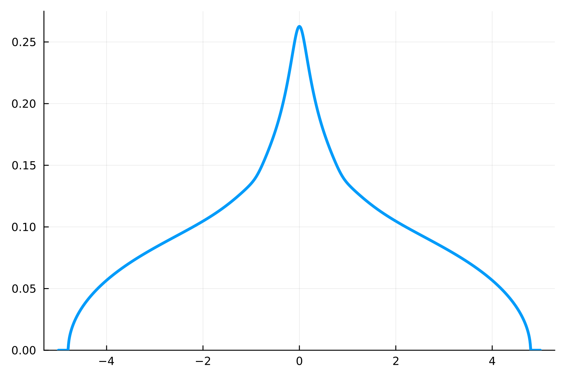
Figure 1. Analytic distribution of $\mu$ computed by numerically applying the Stieltjes inversion formula to its Cauchy transform.

From this it is apparent that there is no atom at zero. In order to prove this rigorously we rely on Proposition 3.1. Figure 2 shows the function $\theta(y):=-y\operatorname{Im}g(iy)$ in logarithmic dependence of the distance $y$ from the real axis.

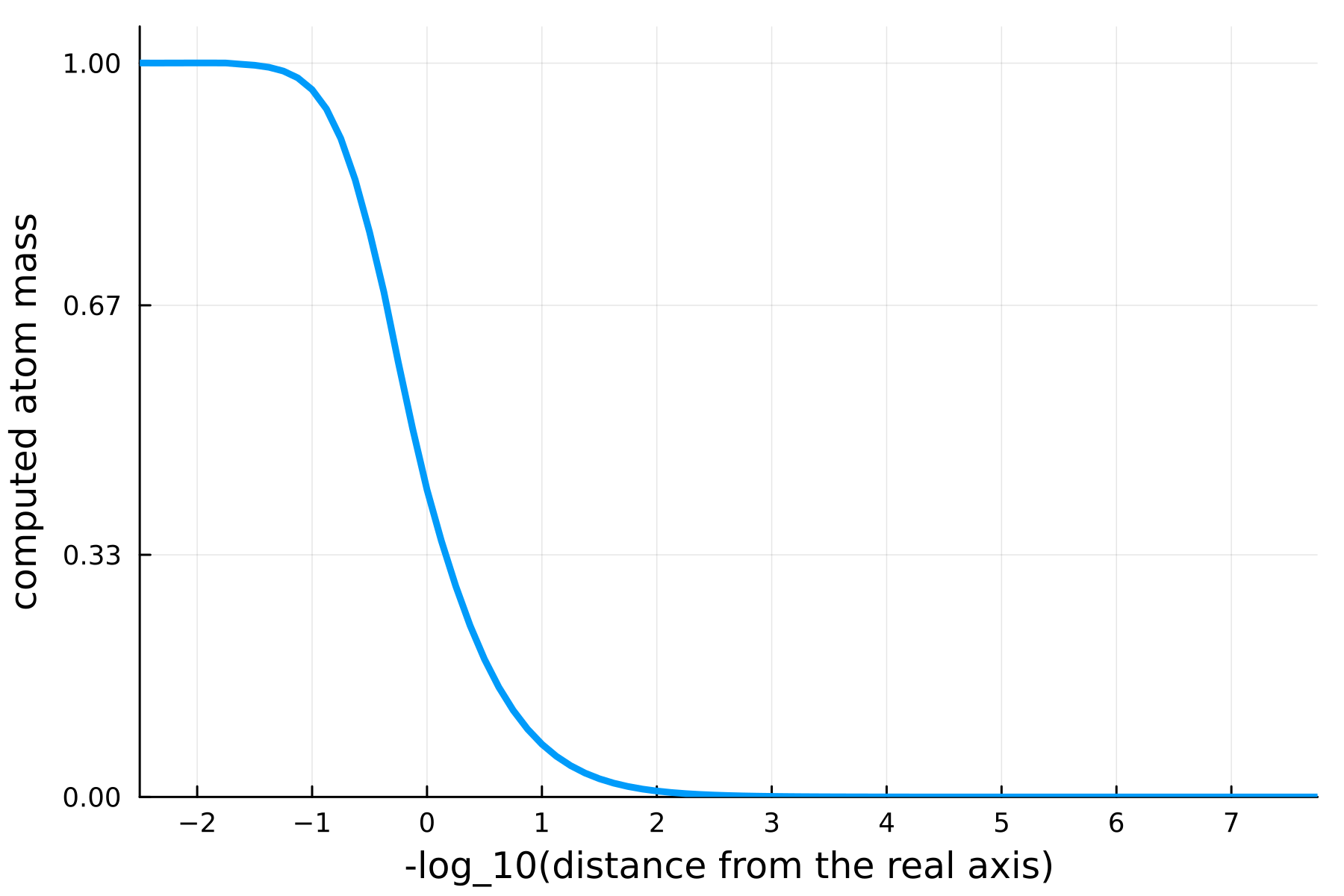
Figure 2. Computed atom mass $\theta(y)$ depending on $y$, which is given by $-\log_{10}(\operatorname{Im}(y))$ (thus $5$ represents a distance of $10^{-5}$ from $y$ to the real axis).

As soon as we fall far enough below (depending on $\varepsilon$) the smallest possible non-trivial size of an atom (which in this case is $1/N=1/3$), we can be sure that there is no atom at 0, and thus the inner rank of $A$ is equal to 3.

6.2. Non-full matrix and some deformations

Let us now consider a non-full example. We take $n=2$ and $N=5$, and consider for two noncommuting variables $\mathbf{x}_{1}$ and $\mathbf{x}_{2}$ the following selfadjoint $5\times 5$ matrix

$$A_{0}=\begin{pmatrix}0&0&0&0&1\\ 0&0&0&0&-4\\ 0&0&0&0&-10\\ 0&0&0&0&-2\\ 1&-4&-10&-2&-1\\ \end{pmatrix}\otimes\mathbf{x}_{1}+\begin{pmatrix}0&0&0&0&7\\ 0&0&0&0&-4\\ 0&0&0&0&7\\ 0&0&0&0&-6\\ 7&-4&7&-6&-7\\ \end{pmatrix}\otimes\mathbf{x}_{2}.$$

In Figure 3 we plot $\theta(y):=-y\operatorname{Im}g(iy)$ for the corresponding Cauchy transform. Since $\theta$ bounds the atom mass from above according to Proposition 3.1 (iii), it becomes apparent from the plot that $\mu(\{0\})\leq 0.6$, corresponding to an inner rank of at least $2$.

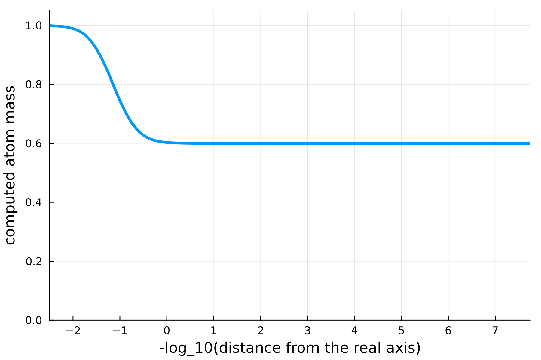
Figure 3. Computed atom mass depending on the distance to the real axis for the unperturbed case $A_{0}$.

It is a well-known fact (see, for example, Proposition 3.1.2 and its proof in [5]) that a matrix of size $m\times n$ with a block of zeros of size $\alpha\times\beta$ has at most inner rank $m+n-\alpha-\beta$. Since $A_{0}$ has a block of zeros of size $4\times 4$, we also get the upper bound $\operatorname{rank}(A_{0})\leq 2$, thus the inner rank of $A_{0}$ is indeed $2$.

Now, we consider two deformations of $A_{0}$. First, we perturb the matrix by a small contribution in the $(1,1)$ entry for the $\mathbf{x}_{1}$ variable, leading to

$$A_{1}=\begin{pmatrix}0.1&0&0&0&1\\ 0&0&0&0&-4\\ 0&0&0&0&-10\\ 0&0&0&0&-2\\ 1&-4&-10&-2&-1\\ \end{pmatrix}\otimes\mathbf{x}_{1}+\begin{pmatrix}0&0&0&0&7\\ 0&0&0&0&-4\\ 0&0&0&0&7\\ 0&0&0&0&-6\\ 7&-4&7&-6&-7\\ \end{pmatrix}\otimes\mathbf{x}_{2}.$$

This increases the inner rank to at least $3$, as can be seen clearly from Figure 4. Since we still have a block of zeros of size $3\times 4$, we also get an upper bound of $3$, which results in $\operatorname{rank}(A_{1})=3$.

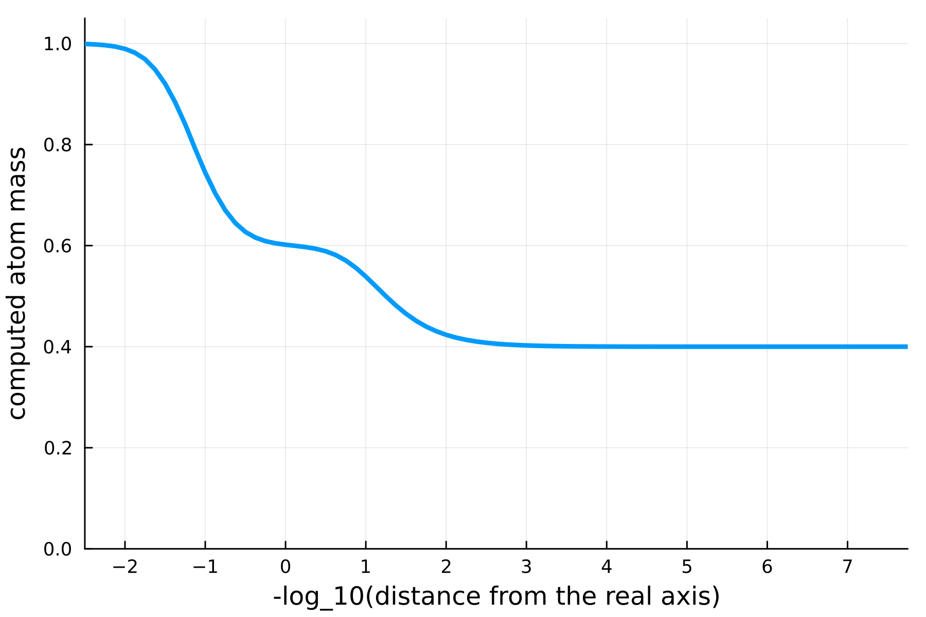
Figure 4. Computed atom mass depending on the distance to the real axis for the first perturbation $A_{1}$.

Second, we add a further perturbation in the $(2,2)$ entry for the $\mathbf{x}_{2}$ variable:

$$A_{2}=\begin{pmatrix}0.1&0&0&0&1\\ 0&0&0&0&-4\\ 0&0&0&0&-10\\ 0&0&0&0&-2\\ 1&-4&-10&-2&-1\\ \end{pmatrix}\otimes\mathbf{x}_{1}+\begin{pmatrix}0&0&0&0&7\\ 0&0.001&0&0&-4\\ 0&0&0&0&7\\ 0&0&0&0&-6\\ 7&-4&7&-6&-7\\ \end{pmatrix}\otimes\mathbf{x}_{2}.$$

Now we only have a block of zeros of size $2\times 4$ and thus an upper bound of $4$ for the inner rank. Finally, from Figure 5 we get $\operatorname{rank}(A_{2})=4$.

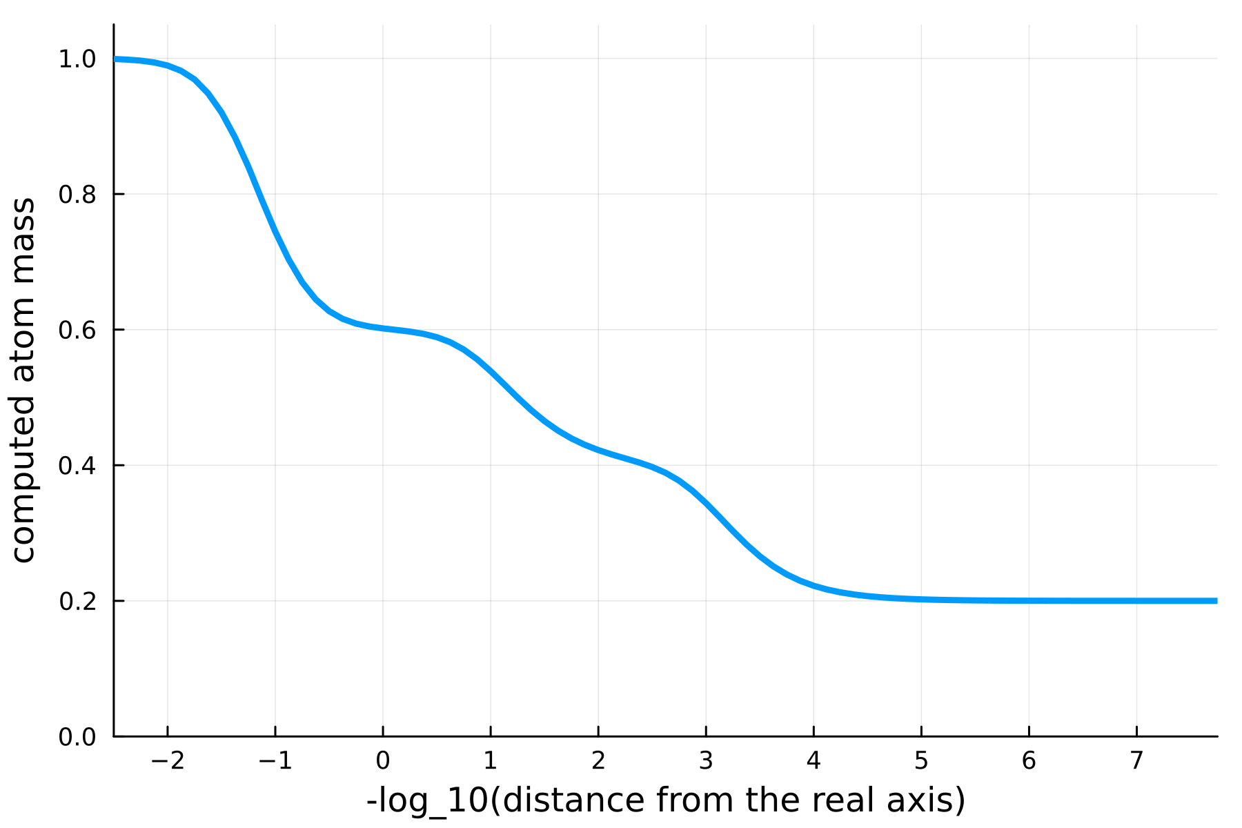
Figure 5. Computed atom mass depending on the distance to the real axis for the second perturbation $A_{2}$.

Note that for all three versions of this example, (3.4) only gives us a lower bound of $2$ for the inner rank. Together with the upper bound from the block structure, this suffices to show that $\operatorname{rank}(A_{0})=2$. For the two deformations, however, the lower bound from (3.4) is not enough to completely determine the inner rank.

References

- BEKS [17] J. Bezanson, A. Edelman, S. Karpinski, and V. B. Shah, Julia: A fresh approach to numerical computing, SIAM Review 59 (2017), no. 1, 65–98.
- Bla [06] B. Blackadar, Operator algebras. Theory of -algebras and von Neumann algebras, Encycl. Math. Sci., vol. 122, Berlin: Springer, 2006.
- BMS [17] S. T. Belinschi, T. Mai, and R. Speicher, Analytic subordination theory of operator-valued free additive convolution and the solution of a general random matrix problem, J. Reine Angew. Math. 732 (2017), 21–53.
- BPV [12] S. T. Belinschi, M. Popa, and V. Vinnikov, Infinite divisibility and a non-commutative Boolean-to-free Bercovici-Pata bijection, J. Funct. Anal. 262 (2012), no. 1, 94–123.
- Coh [06] P. M. Cohn, Free ideal rings and localization in general rings, New Mathematical Monographs, Cambridge University Press, 2006.
- CS [05] A. Connes and D. Shlyakhtenko, -homology for von Neumann algebras, J. Reine Angew. Math. 586 (2005), 125–168.
- EH [70] C. J. Earle and R. S. Hamilton, A fixed point theorem for holomorphic mappings, Global Analysis, Proc. Sympos. Pure Math. 16, 61-65 (1970)., 1970.
- ER [05] A. Edelman and N. R. Rao, Random matrix theory, Acta numerica 14 (2005), 233–297.
- GGOW [16] A. Garg, L. Gurvits, R. Oliveira, and A. Wigderson, A deterministic polynomial time algorithm for non-commutative rational identity testing, 2016 IEEE 57th Annual Symposium on Foundations of Computer Science (FOCS), IEEE, 2016, pp. 109–117.
- GGOW [20] by same author, Operator scaling: theory and applications, Foundations of Computational Mathematics 20 (2020), no. 2, 223–290.
- Har [03] L. A. Harris, Fixed points of holomorphic mappings for domains in Banach spaces, Abstr. Appl. Anal. 2003 (2003), no. 5, 261–274.
- HM [23] J. Hoffmann and T. Mai, NCDist.jl, 2023, https://github.com/johannes-hoffmann/NCDist.jl.
- HMS [18] J. W. Helton, T. Mai, and R. Speicher, Applications of realizations (aka linearizations) to free probability, J. Funct. Anal. 274 (2018), no. 1, 1–79.
- HRS [07] J. W. Helton, R. Rashidi Far, and R. Speicher, Operator-valued semicircular elements: solving a quadratic matrix equation with positivity constraints, Int. Math. Res. Not. 2007 (2007), no. 22, 15.
- KV [14] D. S. Kaliuzhnyi-Verbovetskyi and V. Vinnikov, Foundations of free noncommutative function theory, vol. 199, Providence, RI: American Mathematical Society (AMS), 2014.
- Mai [17] T. Mai, On the analytic theory of non-commutative distributions in free probability, PhD thesis Universität des Saarlandes (2017), 252, https://dx.doi.org/10.22028/D291-26704.
- Mai [22] by same author, The Dyson equation for -positive maps and Hölder bounds for the Lévy distance of densities of states, Preprint, arXiv:2210.04743 [math.FA] (2022), 27.
- MS [17] J. A. Mingo and R. Speicher, Free probability and random matrices., vol. 35, Toronto: The Fields Institute for Research in the Mathematical Sciences; New York, NY: Springer, 2017.
- MSY [23] T. Mai, R. Speicher, and S. Yin, The free field: realization via unbounded operators and Atiyah property, J. Funct. Anal. 285 (2023), no. 5, 50, Id/No 110016.
- NW [22] R. R. Nadakuditi and H. Wu, Free component analysis: Theory, algorithms and applications, Foundations of Computational Mathematics (2022), 1–70.
- PV [13] M. Popa and V. Vinnikov, Non-commutative functions and the non-commutative free Lévy-Hinčin formula, Adv. Math. 236 (2013), 131–157.
- RE [08] N. R. Rao and A. Edelman, The polynomial method for random matrices, Foundations of Computational Mathematics 8 (2008), 649–702.
- Shl [99] D. Shlyakhtenko, -valued semicircular systems, J. Funct. Anal. 166 (1999), no. 1, 1–47.
- Spe [98] R. Speicher, Combinatorial theory of the free product with amalgamation and operator-valued free probability theory, vol. 627, Providence, RI: American Mathematical Society (AMS), 1998.
- SS [15] D. Shlyakhtenko and P. Skoufranis, Freely independent random variables with non-atomic distributions, Trans. Am. Math. Soc. 367 (2015), no. 9, 6267–6291.
- Tak [79] M. Takesaki, Theory of operator algebras I, New York, Heidelberg, Berlin: Springer-Verlag. VII, 415 p., 1979.
- VDN [92] D.-V. Voiculescu, K. J. Dykema, and A. Nica, Free random variables. A noncommutative probability approach to free products with applications to random matrices, operator algebras and harmonic analysis on free groups, CRM Monogr. Ser., vol. 1, Providence, RI: American Mathematical Society, 1992.
- Voi [04] D.-V. Voiculescu, Free analysis questions. I: Duality transform for the coalgebra of , Int. Math. Res. Not. 2004 (2004), no. 16, 793–822.
- Wil [17] J. D. Williams, Analytic function theory for operator-valued free probability, J. Reine Angew. Math. 729 (2017), 119–149.