Control-Oriented Deep Space Communications For Unmanned Space Exploration

Abstract

In unmanned space exploration, the cooperation among space robots requires advanced communication techniques. In this paper, we propose a communication optimization scheme for a specific cooperation system named the “mother-daughter system”. In this setup, the mother spacecraft orbits the planet, while daughter probes are distributed across the planetary surface. During each control cycle, the mother spacecraft senses the environment, computes control commands and distributes them to daughter probes for actions. They synergistically form sensing-communication-computing-control ($\mathbf{SC^{3}}$) loops. Given the indivisibility of the $\mathbf{SC^{3}}$ loop, we optimize the mother-daughter downlink for closed-loop control. The optimization objective is the linear quadratic regulator (LQR) cost, and the optimization parameters are the block length and transmit power. To solve the nonlinear mixed-integer problem, we first identify the optimal block length and then transform the power allocation problem into a tractable convex problem. We further derive the approximate closed-form solutions for the proposed scheme and two communication-oriented schemes: the max-sum rate scheme and the max-min rate scheme. On this basis, we analyze their power allocation principles. In particular, for time-insensitive control tasks, we find that the proposed scheme demonstrates equivalence to the max-min rate scheme. These findings are verified through simulations.

I Introduction

I-A Background and Motivation

Communication plays a vital role in deep space exploration. The link between the spacecraft and the earth command center is the lifeline of the spacecraft. This connection provides tracking, telemetry and command (TT&C) services, which ensure the correct operation. According to the definition of the International Telecommunication Union , if the spacecraft-Earth distance is greater than $2\times 10^{6}$ km, the communication between the spacecraft and the earth belongs to deep space communication (DSC) [1]. Due to the great distance, DSC exhibits unique characteristics. The first is the large latency. Taking Mars as an example, the propagation delay from the perigee of Mars to Earth is 4 minutes, while from the apogee, it is 24 minutes [2]. The second is the low data rate. As a common sense, the signal power decays at least quadratically with distance. To ensure the same strength of the received signals, the transmit power of the spacecraft from Mars should be $9\times 10^{16}$ times stronger than that of a smart phone located 1 km away from the receiver [2]. However, constrained by size and weight limitations, the on-board base station (BS) carried by the spacecraft is less powerful than ground-based facilities. It can only transmit signals at very low power. Ground receivers must be equipped with large aperture antennas to capture the weak signals from space. Even so, the data rate between the spacecraft and the earth command center remains quite low, with only several megabits per second in NASA’s Deep Space Network (DSN) [3].

With the growing curiosity on outer space, current space activities touch the fundamental problems of DSC. The sheer number of space missions is one factor. According to the United Nations, the number of space robots has grown exponentially in the last decade [4]. With advanced sensing techniques, new spacecrafts need a higher data rate to send high-resolution data back, which dramatically increases the burden of the DSN. Moreover, in addition to observation-based explorations, major space powers like the United States, the European Union and China have announced plans to launch execution-based missions such as sample return and base constructions. Unmanned space exploration is evolving from the one that is characterized by an individual spacecraft to the one that relies on network operations. This, however, exceeds the scope of competence of current DSNs.

To ensure that communication enhances rather than constrains unmanned space exploration, the development of space-space communication is essential for robotic cooperation. Without the challenges of long distances, space-space communication facilitates fast and flexible connections among space robots, allowing them to form intelligent cooperation systems. This alleviates the communication burden between the earth segment and the space segment. However, unlike traditional communication networks, the formed cooperation system exhibits prominent task-oriented characteristics. In most cases, space robots operate cyclically: sensors collect surrounding information and report it to the computing unit, the computing unit analyzes the situation and distributes calculated commands to actuators, and the actuators take actions. These robots synergistically form the sensing-communication-computing-control ($\mathbf{SC}^{3}$) loop, which is the basic unit for task execution. Therefore, the communication within the $\mathbf{SC}^{3}$ loop is geared toward serving a specific task rather than achieving a universal data rate.

In this paper, we explore the communication scheme for a specific cooperation system named the “mother-daughter system”. As the name suggests, the “mother-daughter system” consists of one mother spacecraft and multiple daughter probes. In Fig. 1, we illustrate the operational pattern of this system. Upon the launch of a space mission, the mother spacecraft undergoes the launch, transfer orbit, and planet approach phases before reaching the scheduled planetary orbit. Subsequently, the spacecraft releases the lander. Once the lander lands on the planetary surface, it deploys daughter probes. These daughter probes are assigned with various exploration tasks. To enable these relatively less advanced probes to conduct arduous exploration tasks, the mother spacecraft needs to provide real-time guidelines. It carries advanced sensing, communication and computing modules. In each control cycle, the mother spacecraft senses the environment, conducts analysis, and sends instructions to daughter probes to take actions. Together, they synergistically form $\mathbf{SC}^{3}$ loops, serving as the fundamental unit for task execution. Moreover, the adaptable orchestration of the “mother-daughter system” can further give rise to a large-scale exploration network.

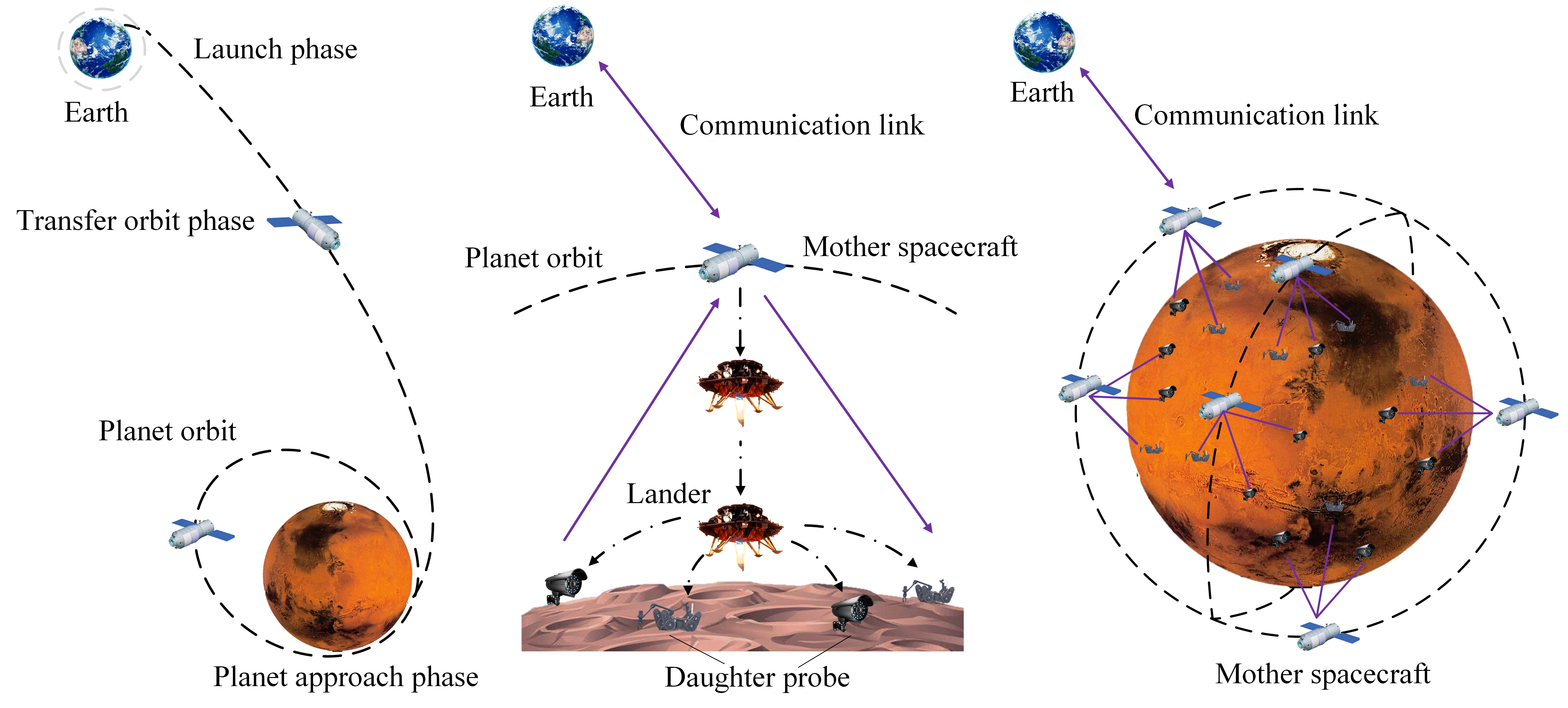
Figure 1: Illustration of the “mother-daughter system” in unmanned space exploration.

In the literature, few studies have investigated space communication from the perspective of the $\mathbf{SC}^{3}$ loop. Communication researchers mostly take the communication link as the investigated objective and address the unique challenges in DSC [5]. While improving communication performance is crucial for space exploration, separating the communication process from the $\mathbf{SC^{3}}$ loop might not be optimal. This approach overlooks the communication impact on the overall functioning of the $\mathbf{SC^{3}}$ loop. In contrast, researchers in control have studied the whole $\mathbf{SC^{3}}$ loop. Specifically, in networked control systems (NCSs), where sensors, controllers, and actuators are interconnected via a shared network, studies showed that communication imperfections can adversely affect the closed-loop control [6]–[8]. In the following, we review related studies of DSC and NCS.

I-B Related Works

I-B1 DSC

DSC plays an important role in unmannd space exploration. Due to the long transmission distance, there exist unique challenges for DSC. Related studies have addressed different challenges from different perspectives, including communication protocols, networking, and resource optimization. For example, Ha et al. proposed a reinforcement learning-based link selection strategy to improve the streaming performance of DSC [9]. To tackle the solar scintillation effect, Xu et al. devised a dual-hop mixed communication system, which comprises a radio frequency link between the earth and the relay satellite and a free-space optical link between the satellite and a deep space probe [10]. To address the challenge of intermittent connections, the delay-tolerant network (DTN) has been developed, in which the store-and-forward strategy is used to combat the interruption. On this basis, Yang et al. proposed a hybrid bundle retransmission scheme to ensure the DTN reliability [11]. Rango et al. proposed an adaptive bundle rate scheme to tackle concurrent bundle transmissions [12]. In terms of the network structure, Wan et al. proposed a satellite relay constellation network and detailed the mathematical model, topology design and performance analysis [13]. These studies have improved the communication performance in deep space, providing a solid foundation for unmanned space exploration.

I-B2 NCS

Taking communication imperfections, such as delays, dropouts, and rate limitations into account, researchers in control have paid great attention to the relationship between communication and control. For example, Tatikonda et al. investigated the minimal data-rate requirement to stabilize the linear time-invariant system [14]. It was proven that only when the data rate exceeds the intrinsic entropy, can the system be stabilized [15]. Afterward, Nair et al. extended this result to nonlinear systems [16]. Kostina et al. further generalized these results to vectorial, non-Gaussian, and partially observed systems. Given the data rate, the authors derived the lower bound of the control linear quadratic regulator (LQR) cost [17].

Building upon these results, numerous resource optimization schemes have been proposed for NCSs. For example, Lyu et al. devised a control-aware cooperative transmission scheme that jointly optimized channel allocation, power control, and relay cooperation [18]. Girgis et al. provided a prediction-based control scheme to minimize the age of information and transmit power [19]. Chang et al. optimized the bandwidth, transmit power, and control convergence rate to maximize the spectrum efficiency [20]. Yang et al. developed a framework to optimize a new metric named the energy-to-control efficiency [21]. Lei et al. proposed a multi-loop optimization scheme to minimize the sum LQR cost. The transmit power was balanced among different loops [22]. Esien et al. proposed a control-aware scheduling scheme that adapted transmissions to channel dynamics and system states [23]. While these works took a first step to orchestrate communication resources for the closed-loop control, they were still preliminary. Some overlooked the fact that the communication within the $\mathbf{SC^{3}}$ loop has stringent latency requirement and did not model the data transmission in the finite block length (FBL) regime, and some remain to take communication metrics as the objective.

I-C Main Contributions

In this paper, we consider a space cooperation system named the “mother-daughter system”, which applies $\mathbf{SC^{3}}$ loops to execute a control-type exploration task. To improve the control performance of these $\mathbf{SC^{3}}$ loops, we propose a control-oriented communication scheme. The main contributions are listed as follows.

1. We propose a control-oriented communication scheme for the “mother-daughter system”. Considering the cycle-time constraint, we model the mother-daughter downlink in the FBL regime. The proposed scheme takes the LQR cost as the objective. The optimized variables are the block length and transmit power.

2. To solve the nonlinear integer problem, we first derive the optimal block length based on the monotonicity of the rate-cost objective function. Subsequently, we analyze the monotonicity and concavity-convexity of the achievable rate expression and the rate-cost function. Building upon these insights, we transform the power allocation problem into a tackle convex problem.

3. In the assure-to-be-stable region, we derive approximate closed-form solutions for the proposed scheme, as well as for two communication-oriented schemes: the max-sum rate scheme and the max-min rate scheme. By showing the equivalence between the proposed scheme and the max-min rate scheme for time-insensitive control tasks, we reveal the fairness-minded nature of the proposed scheme.

4. We use appropriate parameters to model the space environment in the simulation. Simulation results confirm the effectiveness of the proposed scheme in improving the control performance of the $\mathbf{SC^{3}}$ loops and validate our findings.

I-D Organization and Notation

The rest of this paper is organized as follows. Section II introduces the model of the “mother-daughter system” and the $\mathbf{SC^{3}}$ loop. Section III presents the control-oriented communication optimization scheme and its solution. Section IV derives the closed-form solution of the proposed scheme and compares it with that of the max-sum rate scheme and max-min rate scheme. Section V presents simulation results. Section VI draws conclusions.

Throughout this paper, vectors and matrices are represented by lower and upper boldface symbols. $\mathbb{R}^{m\times m}$ represents the set of $m\times m$ real matrices, $\mathbf{I}_{m}$ is the $m\times m$ unit matrix, and $\mathbf{0}_{m}$ is the $m\times m$ zero matrix. $\lambda(\mathbf{A})$ denotes the eigenvalue of matrix $\mathbf{A}$.

II System Model

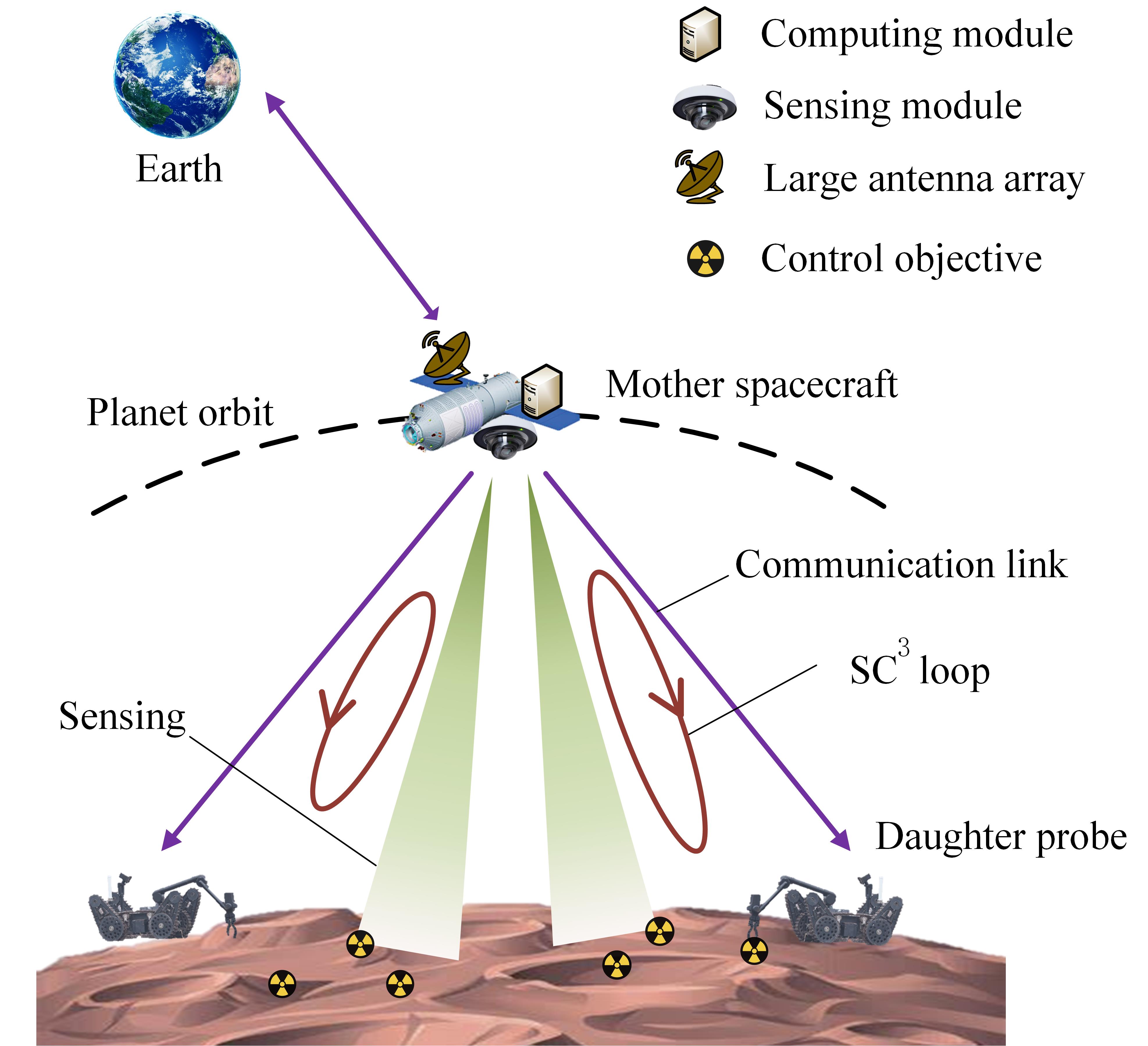
Figure 2: Illustration of an unmanned space cooperation system that comprises a mother spacecraft and multiple daughter probes. The spacecraft and probes synergistically form multiple $\mathbf{SC^{3}}$ loops, and each loop takes charge of a control-type subtask.

In Fig. 2, we present the model of the “mother-daughter system”. The mother spacecraft is located in the planet’s orbit and carries advanced sensing, communication and computing modules. In each control cycle, it senses system states, calculates control commands and distributes these commands to daughter probes for actions. Working in a cyclical manner, they synergically form multiple $\mathbf{SC^{3}}$ loops. The mother spacecraft also maintains a communication link with the earth, which serves for TT&C purposes and sends crucial data back to the earth. We assume that this “mother-daughter system” includes $K$ $\mathbf{SC^{3}}$ loops. Each $\mathbf{SC^{3}}$ loop operates an LQR-based controller to execute a control-type task. For the $k$ th $\mathbf{SC^{3}}$ loop at time index $i$, the following state-space equation is used to characterize the dynamics of the controlled system,

$$\mathbf{x}_{k,i+1}=\mathbf{A}_{k}\mathbf{x}_{k,i}+\mathbf{B}_{k}\mathbf{u}_{k,i}+\mathbf{v}_{k,i},$$ (1)

where $\mathbf{x}_{k,i}\in\mathbb{R}^{m\times 1}$ is the system state and $\mathbf{u}_{k,i}\in\mathbb{R}^{m\times 1}$ is the control input. The matrices $\mathbf{A}_{k}\in\mathbb{R}^{m\times m}$ and $\mathbf{B}_{k}\in\mathbb{R}^{m\times m}$ are determined by the system dynamics, and $\mathbf{v}_{k,i}\in\mathbb{R}^{m\times 1}$ is the system uncertainty, whose covariance matrix is denoted as $\mathbf{\Sigma}_{\mathbf{v}_{k}}\in\mathbb{R}^{m\times m}$. The system is unstable $(\lambda(\mathbf{A}_{k})>1)$, and it can be stabilized using $(\mathbf{A}_{k},\mathbf{B}_{k})$. In practice, the state-space equation is non-linear. (1) is obtained by linearizing the system state around the working point. Currently, the LQR controller has been widely applied in space exploration, for tasks like spacecraft maneuvering and formation flying [24]. Although simplified, the linear control model has been proven effective in characterizing the system dynamics.

During each control cycle, the spacecraft first senses system states. The sensing process is modeled as a partially observed process:

$$\mathbf{y}_{k,i}=\mathbf{C}_{k}\mathbf{x}_{k,i}+\mathbf{w}_{k,i},$$ (2)

where $\mathbf{y}_{k,i}\in\mathbb{R}^{m\times 1}$ is the observation state, $\mathbf{C}_{k}\in\mathbb{R}^{m\times m}$ is the observation matrix, and $\mathbf{w}_{k,i}\in\mathbb{R}^{m\times 1}$ is the sensing noise, which conforms to the Gaussian distribution. The covariance matrix of $\mathbf{w}_{k,i}$ is denoted as $\mathbf{\Sigma}_{\mathbf{w}_{k}}=\sigma^{2}_{w}\mathbf{I}_{m}$.

Then, the spacecraft processes sensing data and calculates control commands. Since the LQR-based control is grounded in well-established control theory, the optimal control input, i.e., $\mathbf{u}_{k,i}$, can be calculated by solving a well-defined optimization problem [25].

Afterward, the mother spacecraft functions as the BS, sending control commands to the respective probes. We assume that both the mother spacecraft and daughter probes are equipped with a single antenna. This single-antenna setting can be extended to the multi-antenna setting, in which the control-oriented beamforming is an interesting topic. We do not delve into this case in this paper. The spacecraft uses orthogonal frequency bands to communicate with probes, allowing different $\mathbf{SC}^{3}$ loops to operate simultaneously without co-channel interference. The bandwidth is the same for $K$ loops, which is denoted as $B$. As for the channel model, the near-planet link has similar characteristics as the near-Earth link [26]. We thereby adopt the model of the near-Earth link [27] to characterize the near-planet environment:

$$PL[dB] =P_{Los}[FSPL+SF_{1}]$$ (3)

$$\quad+(1-P_{Los})[FSPL+SF_{2}+CL],$$

where $PL$ is the path loss, $P_{Los}$ is the line-of-sight probability, $SF_{1}$ and $SF_{2}$ are the fading margins reserved for the shadowing fading, and $CL$ is the clutter effect. The specific values of these parameters depend on the planetary conditions, such as the presence of atmosphere and surface dust. $FSPL$ represents the free-space path loss, which is a function of the carrier frequency $f_{c}$ (MHz) and the mother-daughter distance $d_{k}$ (km):

$$FSPL(d_{k},f_{c})\triangleq 32.45+20\log_{10}(f_{c})+20\log_{10}{(d_{k})}.$$ (4)

In addition, we calculate the antenna gain of the mother spacecraft [28]:

$$G_{k}=G_{\max}\big{(}\frac{J_{1}(u_{k})}{2u_{k}}+36\frac{J_{3}(u_{k})}{u_{k}^{3}}\big{)}^{2},$$ (5)

where $J_{1}(\cdot)$ and $J_{3}(\cdot)$ are the first-kind Bessel functions of orders $1$ and $3$, $G_{\max}$ is the maximum antenna gain, and $u_{k}$ is given by

$$u_{k}=\frac{2.07123\sin\theta_{k}}{\sin\theta_{\text{3dB}}},$$ (6)

where $\theta_{\text{3dB}}$ is the one-sided half-power beam width and $\theta_{k}$ is the off-axis angle. Based on (3) and (5), the channel gain $g_{k}$ of the mother-daughter downlink is given by

$$g_{k}=G_{k}10^{\frac{-PL[dB]}{10}}.$$ (7)

In the considered scenario, the spacecraft must send commands to the probes within the cycle time. These commands need to be encoded by short channel codes, which renders rate losses. According to [29], the achievable rate in the FBL regime can be approximated into

$$r(n_{k},p_{k})\approx\log_{2}(1+\frac{g_{k}p_{k}}{\sigma^{2}})-\sqrt{\frac{V(p_{k})}{n_{k}}}Q^{-1}(\epsilon_{k})\quad(\text{bit/channel use}),$$ (8)

where $n_{k}$ is the block length, $p_{k}$ is the transmit power, $\log_{2}(1+\frac{g_{k}p_{k}}{\sigma^{2}})$ is the Shannon capacity, and $\epsilon_{k}$ is the transmit error probability. $Q^{-1}(\cdot)$ is the inverse of the $Q$ function, i.e., $Q(x)=\frac{1}{\sqrt{2\pi}}\int_{x}^{\infty}e^{-\frac{t^{2}}{2}}dt$, and $V(p_{k})$ is the channel dispersion, which is approximated by the following expression [30]

$$V(p_{k})\approx(\log_{2}e)^{2}\big{(}1-\frac{1}{(1+\frac{g_{k}p_{k}}{\sigma^{2}})^{2}}\big{)}.$$ (9)

In information theory, one channel use corresponds to transmitting one complex symbol. Therefore, the block length $n_{k}$ serves as the number of transmit symbols and the channel use. Based on (8), when using a $n_{k}$-length packet to send the command, the transmit bits are calculated by the following expression:

$$R(n_{k},p_{k})\approx(1-\epsilon_{k})\big{(}n_{k}\log_{2}(1+\frac{g_{k}p_{k}}{\sigma^{2}})-\sqrt{n_{k}V(p_{k})}Q^{-1}(\epsilon_{k})\big{)},$$ (10)

where we denote $R(n_{k},p_{k})$ as the cycle rate, which represents the transmit information per cycle. Obviously, a higher cycle rate facilitates the transmission of more precise control commands, leading to better control performance.

Upon receiving the control command, the probe takes control actions, leading the system to evolve as described by (1). To ensure that the $\mathbf{SC^{3}}$ processes are finished within the cycle time, denoted as $T_{k}^{0}$, it is necessary to satisfy:

$$t_{k}^{s}+t_{k}^{c}+t_{k}^{d}+t_{k}^{a}\leqslant T_{k}^{0},$$ (11)

where $t_{k}^{s}$, $t_{k}^{c}$, $t_{k}^{d}$, and $t_{k}^{a}$ are the time for sensing, computing, downlink communication, and executing control actions. Since we focus on the communication process, the time for sensing, computing and executing control actions is predetermined in this paper. The communication time includes two parts,

$$t_{k}^{d}=\frac{n_{k}}{B}+\tau_{k},n_{k}\in\mathbb{N}^{+},$$ (12)

where $\frac{n_{k}}{B}$ is the transmission delay and $\tau_{k}$ is the propagation delay, which is determined by the mother-daughter distance $d_{k}\ (\text{m})$,

$$\tau_{k}=\frac{d_{k}}{c},$$ (13)

where $c\ (\text{m/s})$ is the speed of light. We simplify the cycle-time constraint (11) into a constraint of the block length

$$\frac{n_{k}}{B}\leqslant T_{k},\ n_{k}\in\mathbb{N}^{+},$$ (14)

where

$$T_{k}\triangleq T_{k}^{0}-t_{k}^{s}-t_{k}^{c}-t_{k}^{a}-\tau_{k},$$ (15)

which represents the maximum allowable time for the transmission.

Moving forward, we use the LQR cost to measure the control performance of the $\mathbf{SC}^{3}$ loop, which is calculated by

$$l_{k}=\limsup\limits_{N\rightarrow\infty}\mathbb{E}\left[\sum_{i=1}^{N}\left(\mathbf{x}_{k,i}^{\text{T}}\mathbf{Q}_{k}\mathbf{x}_{k,i}+\mathbf{u}_{k,i}^{\text{T}}\mathbf{R}_{k}\mathbf{u}_{k,i}\right)\right],$$ (16)

where $\mathbf{Q}_{k}$ and $\mathbf{R}_{k}$ are positive semidefinite matrices. They are used to balance the cost of the state derivation and control input. According to [15], the cycle rate needs to satisfy the following stable condition such that the controlled system can be stabilized,

$$R(n_{k},p_{k})\geqslant\log_{2}|\det\mathbf{A}_{k}|,\ \forall k,$$ (17)

where $\log_{2}|\det\mathbf{A}_{k}|$ is the intrinsic entropy, which quantifies the system instability level. On the premise that (17) is satisfied, the finite cycle rate constructs a lower bound of the LQR cost [17]:

$$l_{k}\geqslant \frac{m|\det\mathbf{N}_{k}\mathbf{M}_{k}|^{\frac{1}{m}}}{2^{\frac{2}{m}(R(n_{k},p_{k})-\log_{2}|\det\mathbf{A}_{k}|)}-1}$$ (18)

$$\quad+\text{tr}\left(\mathbf{\Sigma}_{\mathbf{v}_{k}}\mathbf{S}_{k}\right)+\text{tr}(\mathbf{\Sigma}_{k}\mathbf{A}_{k}^{T}\mathbf{M}_{k}\mathbf{A}_{k}),$$

where

$$\mathbf{S}_{k} =\mathbf{Q}_{k}+\mathbf{A}_{k}^{\text{T}}\left(\mathbf{S}_{k}-\mathbf{M}_{k}\right)\mathbf{A}_{k},$$ (19a)

$$\mathbf{M}_{k} =\mathbf{S}_{k}^{T}\mathbf{B}_{k}\left(\mathbf{R}_{k}+\mathbf{B}_{k}^{T}\mathbf{S}_{k}\mathbf{B}_{k}\right)^{-1}\mathbf{B}_{k}^{\text{T}}\mathbf{S}_{k},$$ (19b)

$$\mathbf{N}_{k} =\mathbf{A}_{k}\mathbf{\Sigma}_{k}\mathbf{A}_{k}^{T}-\mathbf{\Sigma}_{k}+\mathbf{\Sigma}_{\mathbf{v}_{k}}.$$ (19c)

$\mathbf{\Sigma}_{k}$ is calculated by

$$\mathbf{\Sigma}_{k}=\mathbf{P}_{k}-\mathbf{P}_{k}\mathbf{C}_{k}^{T}(\mathbf{C}_{k}\mathbf{P}_{k}\mathbf{C}_{k}^{T}+\mathbf{\Sigma}_{\mathbf{w}_{k}})^{-T}\mathbf{C}_{k}\mathbf{P}_{k}^{T},$$ (20)

where $\mathbf{P}_{k}$ is the solution to the algebraic Riccati equation:

$$\mathbf{P}_{k}= \mathbf{A}_{k}\mathbf{P}_{k}\mathbf{A}_{k}^{T}+\mathbf{\Sigma}_{\mathbf{v}_{k}}$$ (21)

$$\quad-\mathbf{A}_{k}\mathbf{P}_{k}\mathbf{C}_{k}^{T}(\mathbf{C}_{k}\mathbf{P}_{k}\mathbf{C}_{k}^{T}+\mathbf{\Sigma}_{\mathbf{w}_{k}})^{-T}\mathbf{C}_{k}\mathbf{P}_{k}^{T}\mathbf{A}_{k}^{T}.$$

Considering (18) is nearly a tight lower bound of the LQR cost [17], we thereby introduce the rate-cost function,

$$L(n_{k},p_{k}) \triangleq\frac{m|\det\mathbf{N}_{k}\mathbf{M}_{k}|^{\frac{1}{m}}}{2^{\frac{2}{m}(R(n_{k},p_{k})-\log_{2}|\det\mathbf{A}_{k}|)}-1}$$ (22)

$$\quad\quad+\text{tr}\left(\mathbf{\Sigma}_{\mathbf{v}_{k}}\mathbf{S}_{k}\right)+\text{tr}(\mathbf{\Sigma}_{k}\mathbf{A}_{k}\mathbf{M}_{k}\mathbf{A}_{k}),$$

which establishes a bridge between the limit LQR cost and the cycle rate. This connection allows us to orchestrate communication resources for the closed-loop control, which is detailed in the next Section.

III Control-Oriented Optimization of the Mother-Daughter Downlink

Restricted by payload limitations, the spacecraft usually carries lightweight BSs, which are less powerful than ground-based facilities. The restricted transmit power of the onboard BS, coupled with the cycle-time constraint leads to the limited cycle rate of the mother-daughter downlink. This influences the accuracy of transmit commands and affects the control performance. To alleviate the bottleneck effect of mother-daughter downlink in the $\mathbf{SC^{3}}$ loop, we propose a control-oriented communication scheme. This scheme optimizes the block length and transmit power of the mother-daughter to minimize the sum LQR cost of the $K$ $\mathbf{SC^{3}}$ loops,

$$\mbox{(P1)}\ \ \min_{\mathbf{n},\mathbf{p}}\ \ \sum_{k=1}^{K}L(n_{k},p_{k})$$ (23a)

s.t. $$R(n_{k},p_{k})\geqslant\log_{2}|\det\mathbf{A}_{k}|,\ \forall k,$$ (23b)

$$\frac{n_{k}}{B}\leqslant T_{k},n_{k}\in\mathbb{N}^{+},\ \forall k,$$ (23c)

$$\sum_{k=1}^{K}p_{k}\leqslant P_{\text{max}},$$ (23d)

$$p_{k}\geqslant 0,\forall k,$$ (23e)

where $\mathbf{n}\triangleq\{n_{1},...,n_{K}\}$ and $\mathbf{p}\triangleq\{p_{1},...,p_{K}\}$. (P1) is a nonlinear mixed-integer problem. Directly solving it bears high complexity. First, the optimal block length is determined by $T_{k}$,

$$n^{*}_{k}=\lfloor BT_{k}\rfloor.$$ (24)

This is because $L(n_{k},p_{k})$ is a decreasing function of $n_{k}$. It can be proven by the rule of the monotonicity of composite functions, as the rate-cost function decreases with the cycle rate and the cycle rate increases with the block length. After determining the block length, the remaining power allocation problem is given by

$$\mbox{(P2)}\ \ \min_{\mathbf{p}}\ \ \sum_{k=1}^{K}L(p_{k})$$ (25a)

s.t. $$R(p_{k})\geqslant\log_{2}|\det\mathbf{A}_{k}|,\ \forall k,$$ (25b)

$$\sum_{k=1}^{K}p_{k}\leqslant P_{\text{max}},$$ (25c)

$$p_{k}\geqslant 0,\forall k,$$ (25d)

where $R(p_{k})\triangleq R(n_{k}^{*},p_{k})$ and $L(p_{k})\triangleq L(n_{k}^{*},p_{k})$. To solve this problem, we first analyze their monotonicity and convexity-concavity. For the cycle rate $R(p_{k})$, we analyze the property of the achievable rate expression, i.e., $r(p_{k})\triangleq r(n_{k}^{*},p_{k})$, as given in (8), which holds the same property as $R(p_{k})$. For ease of expression, we rewrite $r(p_{k})$ as a function of the signal-to-noise ratio (SNR), denoted as $\gamma_{k}\triangleq\frac{g_{k}p_{k}}{\sigma^{2}}$,

$$r(\gamma)=\log_{2}(1+\gamma)-\eta\sqrt{V(\gamma)},$$ (26)

where $\eta\triangleq\sqrt{\frac{1}{n^{*}}}Q^{-1}(\epsilon)$ and the subscript $k$ is omitted for simplicity. Since the data rate cannot be negative in practice, we discuss the monotonicity and concavity-convexity in the region of $r(\gamma)\geqslant 0$, which is given by Theorem 1.

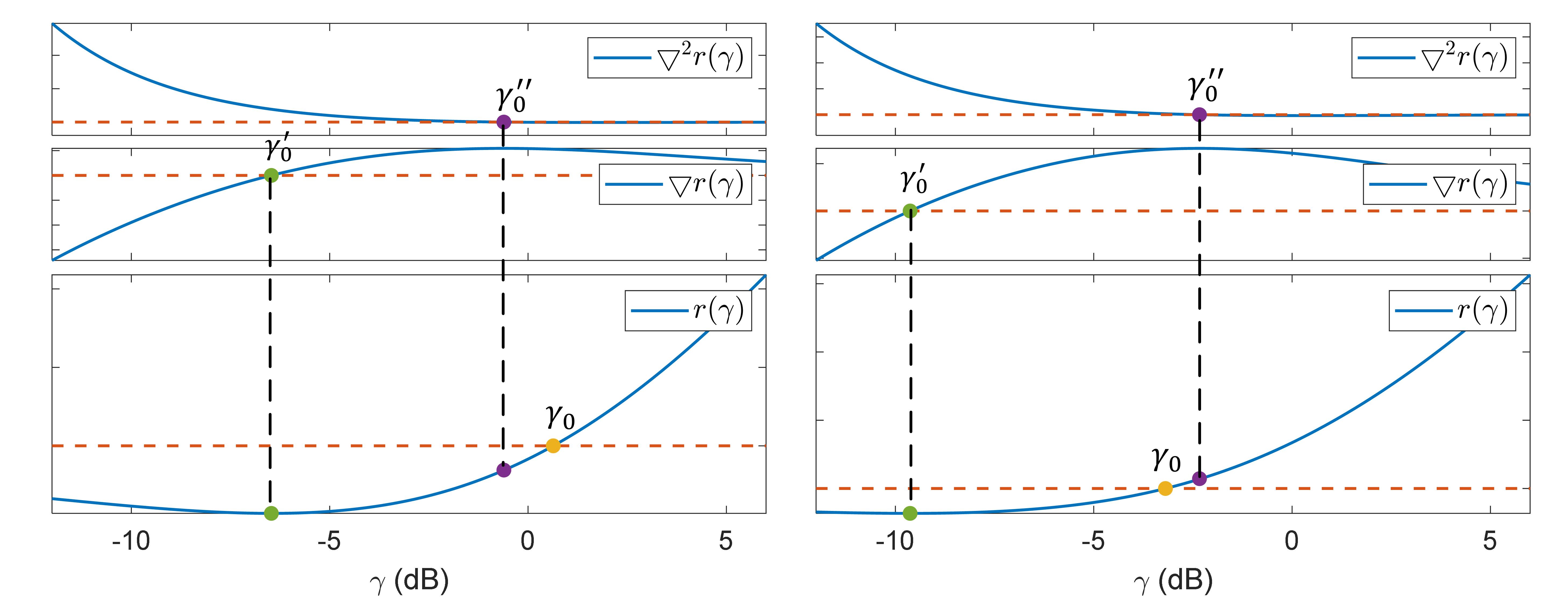
Figure 3: Curves of the achievable rate in the FBL regime, i.e., $r(\gamma)$, its first derivative, i.e., $\triangledown r(\gamma)$, and second derivative, i.e., $\triangledown^{2}r(\gamma)$. Related parameters are set as: $\epsilon=10^{-6}$ and $n=30$ for the left figure, and $\epsilon=10^{-6}$ and $n=80$ for the right figure.

Theorem 1:

Denote the zero-crossing point of $r(\gamma)$ as $\gamma_{0}$ $(\gamma_{0}>0)$.

1. $r(\gamma)$ is monotonically increasing with $\gamma$ in $[\gamma_{0},+\infty)$.

2. The convexity-concavity of $r(\gamma)$ is given by

   $$\left\{\begin{aligned} &r(\gamma)\ \text{is convex-concave in}\ [\gamma_{0},+\infty),\quad\eta<\hat{\eta},\\ &r(\gamma)\ \text{is concave in}\ [\gamma_{0},+\infty),\qquad\qquad\ \eta\geqslant\hat{\eta}.\end{aligned}\right.$$ (27)

   where $\hat{\eta}\triangleq\frac{(1+\hat{\gamma})\ln(1+\hat{\gamma})}{\sqrt{\hat{\gamma}^{2}+2\hat{\gamma}}}$ and $\hat{\gamma}$ is the zero-crossing point of the following equation

   $$\ln(1+\gamma)-\frac{(1+\gamma)(\gamma^{2}+2\gamma)^{2}}{3\gamma^{2}+6\gamma+1}=0.$$ (28)

Proof:

See Appendix A. $\square$

In Fig. 3, we illustrate two examples of $r(\gamma)$ along with its first-order derivative $\triangledown r(\gamma)$ and second-order derivative $\triangledown^{2}r(\gamma)$. The zero-crossing points of $\triangledown r(\gamma)$ and $\triangledown^{2}r(\gamma)$ are denoted as $\gamma_{0}^{\prime}$ and $\gamma_{0}^{\prime\prime}$, respectively. It is noted that $\gamma_{0}^{\prime}$ is the monotonicity turning point of $r(\gamma)$ and $\gamma_{0}^{\prime\prime}$ is the inflection point of $r(\gamma)$. The values of $\gamma_{0}^{\prime}$ and $\gamma_{0}^{\prime\prime}$ compared with $\gamma_{0}$ determine the monotonicity and the concavity-convexity of $r(\gamma)$ in $[\gamma_{0},+\infty)$. Observing both figures, we can see that there is $\gamma_{0}>\gamma_{0}^{\prime}$ in both cases. This shows that $r(\gamma)$ is monotonically increasing in $[\gamma_{0},+\infty)$ in provided examples. Moreover, $r(\gamma)$ demonstrates the concave nature in $[\gamma_{0},+\infty)$ in the left example, as $\gamma_{0}$ exceeds $\gamma_{0}^{\prime\prime}$. Conversely, $r(\gamma)$ is convex-concave in $[\gamma_{0},+\infty)$ in the right example, as $\gamma_{0}$ is smaller than $\gamma_{0}^{\prime\prime}$.

Moving forward, based on the monotonicity of $r(\gamma)$ in $[\gamma_{0},+\infty)$, the constraint (25b) can be simplified into a threshold form

$$p_{k}\geqslant p^{th}_{k},\ \forall k,$$ (29)

where $p^{th}_{k}$ is the solution to the following equation

$$R(p_{k})-\log_{2}|\det\mathbf{A}_{k}|=0.$$ (30)

This solution can be found by the dichotomy method. Thus, (P2) is simplified as

$$\mbox{(P3)}\ \ \min_{\mathbf{p}}\ \ \sum_{k=1}^{K}L(p_{k})$$ (31a)

s.t. $$p_{k}\geqslant p_{k}^{th},\ \forall k,$$ (31b)

$$\sum_{k=1}^{K}p_{k}\leqslant P_{\text{max}}.$$ (31c)

In (P3), the stumbling block in solving the problem is the rate-cost function. It is a composite expression that includes the exponential, fractional, and logarithmic terms. Moving forward, we have Theorem 2.

Theorem 2:

The rate-cost function is a concave function with respect to the transmit power.

Proof:

See Appendix B. $\square$

Based on Theorem 2, we can conclude that (P3) is a convex problem, which can be easily solved by the convex optimization tool. The corresponding algorithm is summarized in Algorithm 1.

IV Comparisons With Two Communication-Oriented Schemes

In this section, we first investigate two communication-oriented schemes for the considered setting. They are the max-sum rate scheme and the max-min rate scheme. On this basis, we compare the proposed control-oriented scheme with these two schemes. Since the optimal block length is calculated using (24), we only focus on the power allocation in this section.

Algorithm 1 Algorithm for Proposed Control-Oriented Communication Scheme

0:   The number of $\mathbf{SC}^{3}$ loops: $K$;Sensing-related parameters: $\mathbf{C}_{k}$ and $\mathbf{\Sigma}_{\mathbf{w}_{k}}$;Communication-related parameters: $B$, $P_{\max}$, $G_{\max}$, $\theta_{\text{3dB}}$, $\epsilon_{k}$, $d_{k}$, $f_{c}$, $\sigma^{2}$, $P_{Los}$, $SF_{1/2}$, and $CL$;Control-related parameters: $\mathbf{A}_{k}$, $\mathbf{B}_{k}$, $\mathbf{Q}_{k}$, $\mathbf{R}_{k}$, $\mathbf{\Sigma}_{\mathbf{v}_{k}}$, and $m$;Cycle time: $T_{k}^{0}$ and the time for sensing, computing, and executing control actions: $t_{k}^{s}$, $t_{k}^{c}$, and $t^{a}_{k}$.

1:  Calculate the maximum allowable time for transmission, i.e., $T_{k}$, according to (15);

2:  Calculate $\mathbf{S}_{k}$, $\mathbf{M}_{k}$, $\mathbf{N}_{k}$, and $\mathbf{\Sigma}_{k}$ according to (19)-(21);

3:  Calculate the optimal block length $n_{k}^{*}$ according to (24);

4:  Calculate the stable condition threshold $p_{k}^{th}$ according to (30);

5:  Obtain the optimal transmit power $p_{k}^{*}$ by solving (P3);

5:  the optimal block length $n_{k}^{*}$ and transmit power $p_{k}^{*}$.

IV-A Communication-Oriented Power Allocation

If we solely chase the optimum of communication, the data rate is a key metric that reflects the communication efficiency. The max-sum rate scheme and max-min rate scheme are two classical communication-oriented schemes. For the considered setting, the corresponding optimization problems are given by

$$\mbox{(PA)}\ \max_{\mathbf{p}}\ \sum\limits_{k=1}^{K}R(p_{k})$$ (32a)

s.t. $$\ R(p_{k})\geqslant\log_{2}|\text{det}\mathbf{A}_{k}|,\ \forall k,$$ (32b)

$$\sum_{k=1}^{K}p_{k}\leqslant P_{\max},$$ (32c)

$$p_{k}\geqslant 0,\forall k.$$ (32d)

$$\mbox{(PB)}\ \max\limits_{\mathbf{p}}\min_{k}\ \ R(p_{k})$$ (33a)

s.t. $$R(p_{k})\geqslant\log_{2}|\text{det}\mathbf{A}_{k}|,\ \forall k,$$ (33b)

$$\sum_{k=1}^{K}p_{k}\leqslant P_{\max}$$ (33c)

$$p_{k}\geqslant 0,\forall k.$$ (33d)

As stated in Theorem 1, the cycle rate $R(p_{k})$ is not necessarily concave with respect to the transmit power. This indicates that (PA) and (PB) are both non-convex. To address this obstacle, we employ Taylor expansion to linearize the nonconvex term of the cycle rate, i.e., $\sqrt{V(p_{k})}$. The first-order Taylor expansion at the given point $\hat{p}_{k}$ is given by

$$R(p_{k}|\hat{p}_{k}) =(1-\epsilon_{k})\big{[}n_{k}^{*}\log_{2}(1+\frac{g_{k}p_{k}}{\sigma^{2}})-$$ (34)

$$\sqrt{n_{k}^{*}}Q^{-1}(\epsilon_{k})\big{(}\sqrt{V(\hat{p}_{k})}+\bigtriangledown\sqrt{V(\hat{p}_{k})}(p_{k}-\hat{p}_{k})\big{)}\big{]},$$

where

$$\bigtriangledown\sqrt{V(\hat{p}_{k})}=\frac{\log_{2}(e)\frac{g_{k}}{\sigma^{2}}}{(1+\frac{g_{k}\hat{p}_{k}}{\sigma^{2}})^{2}\sqrt{(\frac{g_{k}\hat{p}_{k}}{\sigma^{2}})^{2}+2\frac{g_{k}\hat{p}_{k}}{\sigma^{2}}}}.$$ (35)

On this basis, we can solve (PA) and (PB) in an iterative way. The problems at the $i$ th iteration are formulated as

$$\mbox{(PA-2)}\ \max_{\mathbf{p}}\ \sum\limits_{k=1}^{K}R(p_{k}|p_{k}^{i-1})$$ (36a)

s.t. $$\ p_{k}\geqslant p_{k}^{th},\ \forall k,$$ (36b)

$$\sum_{k=1}^{K}p_{k}\leqslant P_{\max}.$$ (36c)

$$\mbox{(PB-2)}\ \max_{\mathbf{p}}\min_{k}\ \ R(p_{k}|p_{k}^{i-1}),$$ (37a)

s.t. $$\ p_{k}\geqslant p_{k}^{th},\ \forall k,$$ (37b)

$$\sum_{k=1}^{K}p_{k}\leqslant P_{\max}.$$ (37c)

where (36b) and (37b) are derived from the stable condition (30) and $p_{k}^{i-1}$ is the solution obtained in the $(i-1)$ th iteration. The algorithm is assured to converge for the monotonicity and boundedness of generated solutions. We summarize the corresponding algorithm in Algorithm 2.

Algorithm 2 Algorithm for the Max-Sum Rate and Max-Min Rate Schemes

0:   The number of $\mathbf{SC}^{3}$ loops: $K$;Sensing-related parameters: $\mathbf{C}_{k}$ and $\mathbf{\Sigma}_{\mathbf{w}_{k}}$;Communication-related parameters: $B$, $P_{\max}$, $G_{\max}$, $\theta_{\text{3dB}}$, $\epsilon_{k}$, $d_{k}$, $f_{c}$, $\sigma^{2}$, $P_{Los}$, $SF_{1/2}$, and $CL$;Control-related parameters: $\mathbf{A}_{k}$, $\mathbf{B}_{k}$, $\mathbf{Q}_{k}$, $\mathbf{R}_{k}$, $\mathbf{\Sigma}_{\mathbf{v}_{k}}$, and $m$;Cycle time: $T_{k}^{0}$ and the time for sensing, computing, and executing control actions: $t_{k}^{s}$, $t_{k}^{c}$, and $t^{a}_{k}$;Iteration termination threshold: $\delta$.

1:  Calculate the maximum allowable time for transmission, i.e., $T_{k}$, according to (15);

2:  Calculate $\mathbf{S}_{k}$, $\mathbf{M}_{k}$, $\mathbf{N}_{k}$, and $\mathbf{\Sigma}_{k}$ according to (19)-(21);

3:  Calculate the optimal block length $n_{k}^{*}$ according to (24);

4:  Calculate the stable condition threshold $p_{k}^{th}$ according to (30);

5:  Initialization: $i=0$ and $p_{k}^{0}=p_{k}^{th}$;

6:  repeat

7:     $i=i+1$;

8:     Obtain $p_{k}^{(i)}$ by solving (PA-2) and (PB-2);

9:  until $\frac{\absolutevalue{\sum\limits_{k=1}^{K}R(p_{k}^{(i)})-\sum\limits_{k=1}^{K}R(p_{k}^{(i-1)})}}{\sum\limits_{k=1}^{K}R(p_{k}^{(i-1)})}\leqslant\delta$ for (PA); $\quad\quad\ \frac{\absolutevalue{\min\limits_{k}R(p_{k}^{(i)})-\min\limits_{k}R(p_{k}^{(i-1)})}}{\min\limits_{k}R(p_{k}^{(i-1)})}\leqslant\delta$ for (PB).

9:  the optimal block length $n_{k}^{*}$ and transmit power $p_{k}^{*}$.

IV-B Approximate Closed-Form Solutions

In this subsection, we derive the approximate closed-form solutions for three discussed schemes. We assume that all the $\mathbf{SC}^{3}$ loops have the same maximum allowable transmission time, i.e., $T_{k}=T,\forall k$. According to (24), the optimal block length is calculated by $n=\lfloor BT\rfloor$. In addition, on the condition that the received SNR is greater than 5 dB, i.e., $10\log_{10}(\frac{g_{k}p_{k}}{\sigma^{2}})\geqslant 5$ dB, we can approximate the cycle rate, i.e., $R(p_{k})$, as follows [31]

$$R(p_{k})\approx n\log_{2}(1+\frac{g_{k}p_{k}}{\sigma^{2}})-\sqrt{n}\log_{2}(e)Q^{-1}(\epsilon_{k}).$$ (38)

Furthermore, when the system is in the assure-to-be-stable region, where the cycle rate is much larger than the intrinsic entropy, i.e., $R(p_{k})\gg\log_{2}|\det\mathbf{A}_{k}|$, the rate-cost function has the following approximation:

$$L(p_{k}) =\frac{m|\det\mathbf{N}_{k}\mathbf{M}_{k}|^{\frac{1}{m}}}{2^{\frac{2}{m}(R(p_{k})-\log_{2}|\det\mathbf{A}_{k}|)}-1}$$ (39)

$$\quad\quad+\text{tr}\left(\mathbf{\Sigma}_{\mathbf{v}_{k}}\mathbf{S}_{k}\right)+\text{tr}(\mathbf{\Sigma}_{k}\mathbf{A}_{k}\mathbf{M}_{k}\mathbf{A}_{k})$$

$$\approx\frac{m|\det\mathbf{N}_{k}\mathbf{M}_{k}|^{\frac{1}{m}}}{2^{\frac{2}{m}(R(p_{k})-\log_{2}|\det\mathbf{A}_{k}|)}}$$

$$\quad\quad+\text{tr}\left(\mathbf{\Sigma}_{\mathbf{v}_{k}}\mathbf{S}_{k}\right)+\text{tr}(\mathbf{\Sigma}_{k}\mathbf{A}_{k}\mathbf{M}_{k}\mathbf{A}_{k})$$

$$=\frac{m|\det\mathbf{N}_{k}\mathbf{M}_{k}|^{\frac{1}{m}}|\text{det}\mathbf{A}_{k}|^{\frac{2}{m}}e^{\frac{2\sqrt{n}}{m}Q^{-1}(\epsilon_{k})}}{(1+\frac{gp_{k}}{\sigma^{2}})^{\frac{2n}{m}}}$$

$$\quad\quad+\text{tr}\left(\mathbf{\Sigma}_{\mathbf{v}_{k}}\mathbf{S}_{k}\right)+\text{tr}(\mathbf{\Sigma}_{k}\mathbf{A}_{k}\mathbf{M}_{k}\mathbf{A}_{k}).$$

By testing the Slater condition, it is easy to find that the strong duality holds for (P3). Solving its dual problem yields the same optimal solution. The dual problem is given by

$$\mbox{(P4)}\quad\max_{\lambda}\min_{\mathbf{p}}\quad \sum_{k=1}^{K}L(p_{k})+\lambda(\sum_{k=1}^{K}p_{k}-P_{\text{max}})$$ (40a)

s.t. $$\lambda\geqslant 0,$$ (40b)

where $\lambda$ is the Lagrangian multiplier. The stable condition is omitted because it is satisfied in the assure-to-be-stable region. The Karush-Kuhn-Tucker (KKT) conditions of (P4) are given by

$$\frac{\partial L(p_{k})}{\partial p_{k}}+\lambda\bigg{|}_{p_{k}=p_{k}^{*}}=0,\forall k,$$ (41a)

$$\sum_{k=1}^{K}p_{k}-P_{\text{max}}\bigg{|}_{p_{k}=p_{k}^{*}}=0,$$ (41b)

$$\lambda\geqslant 0,$$ (41c)

where the equality of (41b) comes from the monotonicity of $L(p_{k})$. Using the approximation of $L(p_{k})$ in (39), we calculate $\frac{\partial L(p_{k})}{\partial p_{k}}$. Then, (41a) can be reorganized into:

$$p_{k}^{*}(\lambda)=(\frac{\sigma^{2}}{g_{k}})^{\frac{2n}{2n+m}}(\frac{2nG_{k}}{\lambda})^{\frac{m}{2n+m}}e^{\frac{2\sqrt{n}Q^{-1}(\epsilon_{k})}{2n+m}}-\frac{\sigma^{2}}{g_{k}},$$ (42)

where $G_{k}\triangleq|\det\mathbf{N}_{k}\mathbf{M}_{k}|^{\frac{1}{m}}|\det\mathbf{A}_{k}|^{\frac{2}{m}}$, which represents the sensing-and-control-related parameter. By substituting (42) into (41b), we can further obtain that

$$(\frac{1}{\lambda})^{\frac{m}{2n+m}}=\frac{P_{\max}+\sum\limits_{i=1}^{K}\frac{\sigma^{2}}{g_{i}}}{\sum\limits_{i=1}^{K}(\frac{\sigma^{2}}{g_{i}})^{\frac{2n}{2n+m}}(2nG_{i})^{\frac{m}{2n+m}}e^{\frac{2\sqrt{n}Q^{-1}(\epsilon_{i})}{2n+m}}}.$$ (43)

Combining (42) and (43), the closed-form solution to the proposed scheme is derived,

$$p_{k}^{*}=(P_{\max}+\sum_{i=1}^{K}\frac{\sigma^{2}}{g_{i}})\frac{(\frac{\sigma^{2}}{g_{k}})^{\frac{2n}{2n+m}}e^{\frac{2\sqrt{n}Q^{-1}(\epsilon_{k})}{2n+m}}G_{k}^{\frac{m}{2n+m}}}{\sum\limits_{i=1}^{K}(\frac{\sigma^{2}}{g_{i}})^{\frac{2n}{2n+m}}e^{\frac{2\sqrt{n}Q^{-1}(\epsilon_{i})}{2n+m}}G_{i}^{\frac{m}{2n+m}}}-\frac{\sigma^{2}}{g_{k}}.$$ (44)

In addition, when the cycle-time differences of different $\mathbf{SC}^{3}$ loops are not significant, (44) can be applied to the more general case in which different $\mathbf{SC}^{3}$ loops have different cycle time by substituting $n$ with $n_{k}^{*}$.

Moving forward, we derive the closed-form solutions for two communication-oriented schemes. Using the high-SNR approximation in (38), (PA) and (PB) become two convex problems. As for (PA), if without the stable condition (32b), the optimal solution is given by the classical Water-Filling method [32, Ch 9.4]

$$p_{k}^{*}=\big{[}\frac{1}{\lambda}-\frac{\sigma^{2}}{g_{k}}\big{]}^{+},$$ (45)

where $[x]^{+}=\max\{x,0\}$, $\lambda$ is chosen to satisfy $\sum\limits_{k=1}^{K}p_{k}=P_{\max}$. On this basis, it is easy to derive the closed-form solution to (PA) by taking (32b) into account:

$$p_{k}^{*}=\max\bigg{(}\big{[}\frac{1}{\lambda}-\frac{\sigma^{2}}{g_{k}}\big{]}^{+},p_{k}^{th}\bigg{)},$$ (46)

where $\lambda$ is chosen to satisfy $\sum\limits_{k=1}^{K}p_{k}=P_{\max}$.

As for the max-min rate scheme, if there is no stable condition (33b), the optimal solution to (PB) satisfies

$$R(p^{*}_{1})=R(p^{*}_{2})\cdots=R(p^{*}_{K})=\lambda,$$ (47)

where $\lambda$ is an auxiliary variable. This is because if (47) does not hold, the minimal cycle rate among the $K$ $\mathbf{SC}^{3}$ loops could be further improved by reallocating the transmit power from other loops to the loop with the minimum cycle rate. Based on (47), we could derive that

$$p_{k}^{*}=2^{\frac{\lambda}{n}}(\frac{\sigma^{2}}{g_{k}})e^{\frac{Q^{-1}(\epsilon_{k})}{\sqrt{n}}}-\frac{\sigma^{2}}{g_{k}}.$$ (48)

Then, substituting (48) into $\sum\limits_{k=1}^{K}p_{k}^{*}=P_{\max}$, we can obtain that

$$2^{\frac{\lambda}{n}}=\frac{P_{\max}+\sum\limits_{i=1}^{K}\frac{\sigma^{2}}{g_{i}}}{\sum\limits_{i=1}^{K}(\frac{\sigma^{2}}{g_{i}})e^{\frac{Q^{-1}(\epsilon_{i})}{\sqrt{n}}}}.$$ (49)

We further substitute (49) into (48). The closed-form solution is given by

$$p_{k}^{*}=(P_{\max}+\sum\limits_{i=1}^{K}\frac{\sigma^{2}}{g_{i}})\frac{(\frac{\sigma^{2}}{g_{k}})e^{\frac{Q^{-1}(\epsilon_{k})}{\sqrt{n}}}}{\sum\limits_{i=1}^{K}(\frac{\sigma^{2}}{g_{i}})e^{\frac{Q^{-1}(\epsilon_{i})}{\sqrt{n}}}}-\frac{\sigma^{2}}{g_{k}}.$$ (50)

On this basis, it is easy to obtain the closed-form solution to (PB) by taking the stable condition into account,

$$p_{k}^{*}=\max\bigg{[}(\lambda+\sum\limits_{i=1}^{K}\frac{\sigma^{2}}{g_{i}})\frac{(\frac{\sigma^{2}}{g_{k}})e^{\frac{Q^{-1}(\epsilon_{k})}{\sqrt{n}}}}{\sum\limits_{i=1}^{K}(\frac{\sigma^{2}}{g_{i}})e^{\frac{Q^{-1}(\epsilon_{i})}{\sqrt{n}}}}-\frac{\sigma^{2}}{g_{k}},\ p_{k}^{th}\bigg{]},$$ (51)

where $\lambda$ is chosen to satisfy $\sum\limits_{k=1}^{K}p_{k}^{*}=P_{\max}$. In addition, if $P_{\max}$ is large enough such that $p_{k}\geqslant p_{k}^{th}$ is satisfied, the optimal solution is exactly (50).

IV-C Analysis of Power Allocation Principles

Comparing the closed-form solutions of the control-oriented scheme, the max-sum rate scheme and the max-min rate scheme, we have following observations:

1. The proposed control-oriented scheme provides a way to account for sensing and control factors in the communication design. According to (44), the $\mathbf{SC^{3}}$ loops with less accurate sensing and more instability (corresponding to a larger $G_{k}$) are assigned more transmit power. In contrast, the two communication-oriented schemes overlook these crucial factors as they solely focus on the communication process.

2. In terms of channel conditions, the proposed scheme and the max-min rate scheme exhibit a similar power allocation pattern. They allocate more power to the $\mathbf{SC^{3}}$ loops with poorer channel conditions. Conversely, the max-sum rate scheme allocates more power to the $\mathbf{SC^{3}}$ loops with better channel conditions.

Inspired by the similar allocation principle between the control-oriented scheme and the max-min rate scheme in terms of channel conditions, we further find their equivalence for time-insensitive tasks, which is concluded by the following Theorem.

Theorem 3:

When $n\gg m$, the following modified max-min rate scheme yields the same power allocation solution as the control-oriented scheme

$$\mbox{(PC)}\ \max\limits_{\mathbf{p}}\min\limits_{k}\ R(p_{k})-\frac{m}{2}\log_{2}(G_{k})$$ (52a)

s.t. $$R(p_{k})\geqslant\log_{2}|\det\mathbf{A}_{k}|,\ \forall k,$$ (52b)

$$\sum_{k=1}^{K}p_{k}\leqslant P_{\max},$$ (52c)

$$p_{k}\geqslant 0,\forall k.$$ (52d)

In addition, when the optimal block length, i.e., $n$, goes to infinity, the max-min rate scheme yields the same solution as the proposed scheme.

Proof:

When $n\gg m$, we have that $\lim\limits_{n\gg m}2n+m=2n$. Then, the closed-form solution of the proposed scheme (44) has the following approximation:

$$\lim_{n\gg m}\bigg{[}( P_{\max}+\sum_{i=1}^{K}\frac{\sigma^{2}}{g_{i}})\frac{(\frac{\sigma^{2}}{g_{k}})^{\frac{2n}{2n+m}}e^{\frac{2\sqrt{n}Q^{-1}(\epsilon_{k})}{2n+m}}G_{k}^{\frac{m}{2n+m}}}{\sum\limits_{i=1}^{K}(\frac{\sigma^{2}}{g_{i}})^{\frac{2n}{2n+m}}e^{\frac{2\sqrt{n}Q^{-1}(\epsilon_{i})}{2n+m}}G_{i}^{\frac{m}{2n+m}}}-\frac{\sigma^{2}}{g_{k}}\bigg{]},$$ (53)

$$=( P_{\max}+\sum_{i=1}^{K}\frac{\sigma^{2}}{g_{i}})\frac{(\frac{\sigma^{2}}{g_{k}})e^{\frac{Q^{-1}(\epsilon_{k})}{\sqrt{n}}}G_{k}^{\frac{m}{2n}}}{\sum\limits_{i=1}^{K}(\frac{\sigma^{2}}{g_{i}})e^{\frac{Q^{-1}(\epsilon_{i})}{\sqrt{n}}}G_{i}^{\frac{m}{2n}}}-\frac{\sigma^{2}}{g_{k}}.$$

By comparing (53) with the closed-form solution of the max-min rate scheme (50), it is easy to find that (53) is the closed-form solution to the modified max-min problem (PC). In addition, when the block length $n$ goes to infinity, the following approximations can be made:

$$\lim\limits_{n\rightarrow+\infty}\frac{2n}{2n+m}=1,$$ (54)

$$\lim\limits_{n\rightarrow+\infty}\frac{m}{2n+m}=0,$$

$$\lim\limits_{n\rightarrow+\infty}\frac{2\sqrt{n}}{2n+m}=\frac{1}{\sqrt{n}}.$$

Then, the closed-form solution to the proposed scheme (44) can be further simplified into

$$\lim_{n\rightarrow+\infty}\bigg{[} (P_{\max}+\sum_{i=1}^{K}\frac{\sigma^{2}}{g_{i}})\frac{(\frac{\sigma^{2}}{g_{k}})^{\frac{2n}{2n+m}}e^{\frac{2\sqrt{n}Q^{-1}(\epsilon_{k})}{2n+m}}G_{k}^{\frac{m}{2n+m}}}{\sum\limits_{i=1}^{K}(\frac{\sigma^{2}}{g_{i}})^{\frac{2n}{2n+m}}e^{\frac{2\sqrt{n}Q^{-1}(\epsilon_{i})}{2n+m}}G_{i}^{\frac{m}{2n+m}}}-\frac{\sigma^{2}}{g_{k}}\bigg{]},$$ (55)

$$=( P_{\max}+\sum_{i=1}^{K}\frac{\sigma^{2}}{g_{i}})\frac{(\frac{\sigma^{2}}{g_{k}})e^{\frac{Q^{-1}(\epsilon_{k})}{\sqrt{n}}}}{\sum\limits_{i=1}^{K}(\frac{\sigma^{2}}{g_{i}})e^{\frac{Q^{-1}(\epsilon_{i})}{\sqrt{n}}}}-\frac{\sigma^{2}}{g_{k}},$$

which is the same as the solution to the max-min rate scheme, i.e., (50). $\square$

Theorem 3 reveals the fairness-minded nature of the proposed scheme. In fact, to avoid the “short-board effect” that drags down the system efficiency, the proposed scheme guarantees the basic performance of all loops. In addition, the equivalence between the proposed scheme and the max-min rate scheme indicates that as the cycle time increases, the interdependence between communication and control weakens. Under this condition, the max-min rate scheme yields the near-optimal solution for the closed-loop control. Therefore, we can conclude that the proposed scheme is necessary for time-sensitive control tasks, while the max-min rate scheme is a good alternative for time-insensitive cases.

V Simulation Results and Discussion

In the simulation, we assume that there are $K=4$ $\mathbf{SC^{3}}$ loops. For sensing-related parameters, we set $\mathbf{C}_{k}=\mathbf{I}_{m}$ and $\mathbf{\Sigma}_{\mathbf{w}_{k}}=\mathbf{0}_{m}$. For control-related parameters, we set $m=100$, $\mathbf{Q}_{k}=\mathbf{I}_{m}$, $\mathbf{R}_{k}=\mathbf{0}_{m}$, and $\mathbf{\Sigma}_{\mathbf{v}_{k}}=0.01*\mathbf{I_{m}}$ [22]. The intrinsic entropy is given by $\log_{2}|\det\mathbf{A}_{k}|=\{48,36,24,12\}$ for $k=1\sim 4$. The control cycle time is $T_{k}^{0}=50$ ms and the time used for sensing, computing and control is $40$ ms. In this way, the time allowed for communication is 10 ms, which accords to the closed-loop control requirement in space exploration [33]. As for communication-related parameters, each $\mathbf{SC^{3}}$ loop is allocated with a narrow frequency band of $B=15$ kHz. The carrier frequency is $f_{c}=2$ GHz, the variance of the channel noise is $\sigma^{2}=-110$ dBm [22], and the transmission error probability is $\epsilon_{k}=10^{-6}$. The maximal antenna gain is $G_{\max}=23$ dBi and $\theta_{\text{3dB}}=30^{\circ}$. Given that there are no high buildings on the explored planet, we use the rural scenario to model the near-planet environment. The channel-related parameters are given by $P_{Los}=91.9\%$, $SF_{1}=1.14$ dB, $SF_{2}=8.78$ dB and $CL=18.42$ dB [27]. According to the height of the Mars orbit, we set the height of the mother spacecraft to 3000 km and four probes are located $[1000,2000,3000,4000]$ km away from the horizontal projection point of the spacecraft. In the present figures, the dotted line represents the infinite LQR cost and the system is unstable in such cases.

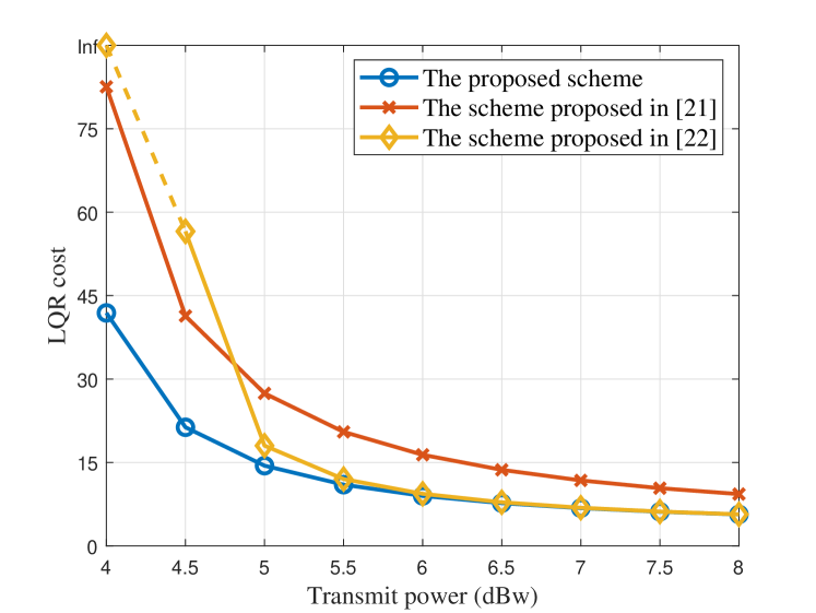
Figure 4: Comparisons of the LQR cost under three control-oriented schemes.

In Fig. 4, we compare the proposed scheme with two control-oriented schemes [21][22]. The scheme in [21] defined a new objective named the energy-to-control efficiency. We thereby use $\frac{P_{\max}-\sum\limits_{k=1}^{K}{p_{k}}}{\sum\limits_{k=1}^{K}L(n_{k},p_{k})}$ as its objective in the simulation. As for the scheme proposed in [22], it took the LQR cost as the objective, but this scheme used the Shannon capacity to calculate the cycle rate. It can be seen that the scheme proposed in [22] performs the worst when $P_{\max}\leqslant 4.5$ dBw. This is attributed to its unawareness of the rate losses in the FBL regime. Some loops that should have been allocated with more power are under allocated. This leads to the system instability in the low power region. As the power increases, the LQR cost under the scheme in [21] becomes the highest. This is due to its emphasis on energy efficiency. The control performance has to make a compromise to save power.

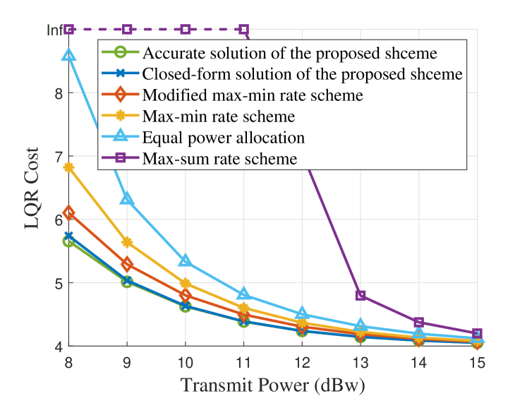
Figure 5: Comparisons of the proposed scheme, the modified max-min rate scheme, the max-min rate scheme, the max-sum rate scheme and equal power allocation.

In Fig. 5, we compare the proposed scheme with three communication-oriented schemes: the max-sum rate scheme, the max-min rate scheme, and the classical equal power allocation. The curves under the approximate closed-form solution of the proposed scheme (44) and the modified max-min rate scheme (PC) are also shown. It can be seen that the control performance using the approximate closed-form solution (44) is nearly the same as that using the accurate solution. The performance under the modified max-min rate scheme shows a small gap from the optimal one. These results confirm their excellent approximations to the optimal solution. In addition, we can also see that the max-min rate scheme outperforms equal power allocation. Both of them further outperform the max-sum rate scheme. This is because of their different power allocation principles in terms of the channel condition. The max-min rate scheme holds a similar allocation principle as the proposed scheme, while the max-sum rate scheme follows an opposite allocation principle.

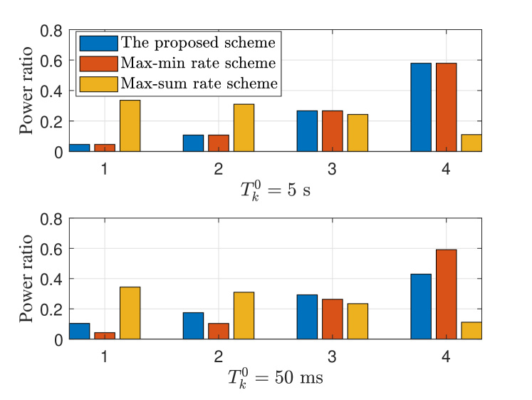
Figure 6: The power allocation results under the proposed scheme, the max-sum rate scheme and the max-min rate scheme.

In Fig. 6, we present the power allocation results of the proposed scheme, the max-sum rate scheme, and the max-min rate scheme. The maximal transmit power is set as $P_{\max}=10$ dBw. It is evident that in both subfigures, the power ratio increases from loops one to four under the proposed scheme and the max-min rate scheme, while it decreases under the max-sum rate scheme. This verifies their power allocation principles in terms of channel conditions. In addition, when the cycle time is $50$ ms, the proposed scheme allocates more power to $\mathbf{SC^{3}}$ loops $1\sim 3$ compared with the max-min rate scheme. This is because we set $\log_{2}|\det\mathbf{A}_{k}|=\{48,36,24,12\}$ for $k=1\sim 4$. This adjustment is made to compensate for the intrinsic entropy difference. In the top subfigure, which shows the case of $T_{k}^{0}=5$ s, the power allocation results of the proposed scheme and the max-min rate scheme are nearly the same. In this situation, the intrinsic entropy difference has little impact on the communication power allocation. This verifies our conclusions drawn in Theorem 3.

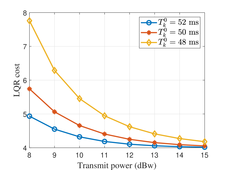
Figure 7: Comparisons of the LQR cost under different cycle time

Next, we discuss the impacts of the cycle time on the control performance. The results are presented in Fig. 7. It can be seen that the cycle time impacts the control performance in the lower power region. As the power increases, different curves converge to the same minimal value. This is because in the low–power region, the cycle rate is very limited. Different cycle time brings with different cycle rates and different accuracy of the commands, which, consequently, leads to different control performances. While in the high-power region, all loops have sufficient cycle rates to deliver commands accurately. The control performances all go to the same optimum, making the cycle time difference less influential in this region.

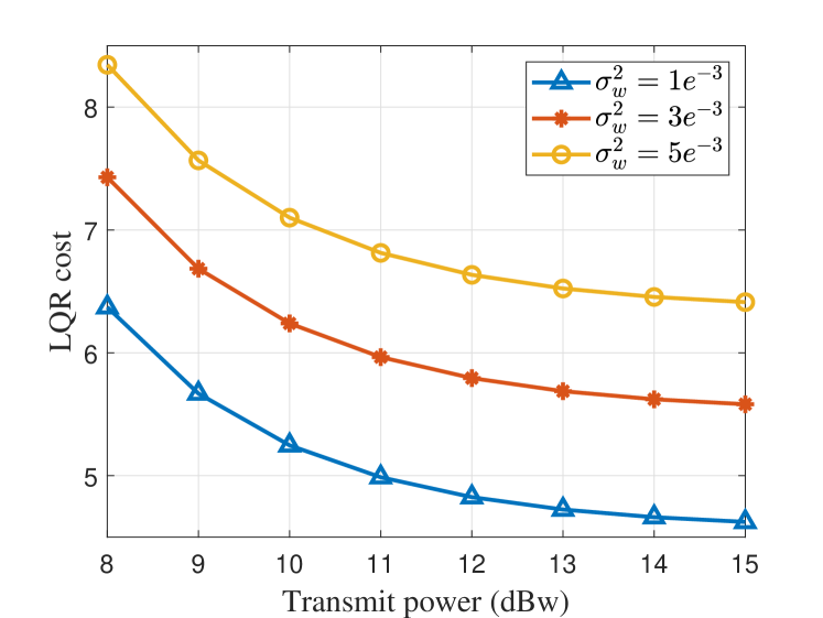
Figure 8: Comparisons of the LQR cost under different sensing noise

In Fig. 8, we present the impacts of the sensing noise on the control performance. Different from the impact of cycle time, the LQR cost under different sensing noise would not converge to the same minimal value as the power increases. This is because inaccurate sensing leads to the control command deviating from the optimal one. This deviation cannot be eliminated regardless of how excellent the communication is. In fact, in the flat region of these curves, the bottleneck of the $\mathbf{SC}^{3}$ loop is sensing but not communication.

VI Conclusions

In this paper, we have investigated a control-oriented communication scheme for a space cooperation system named the “mother-daughter system”. The proposed scheme have optimized the block length and transmit power to minimize the sum LQR cost of the $\mathbf{SC^{3}}$ loops. The mother-daughter downlink has been modeled in the FBL regime. We have solved the nonlinear mixed-integer problem by proving the monotonicity and convexity of the achievable rate expression and the rate-cost function. The approximate closed-form solutions for the control-oriented scheme and two communication-oriented schemes: the max-sum rate scheme and the max-min rate scheme, have been derived. Based on these closed-form solutions, we have revealed the equivalence between the proposed control-oriented scheme and the max-min rate scheme for time-insensitive control tasks. Simulation results have verified the effectiveness of the control-oriented communication scheme in improving the control task performance.

Appendix A Proof of Theorem 1

To prove the monotonicity and concavity-convexity of the achievable rate expression in the FBL regime, i.e., $r(\gamma)$, as shown in (26), we first calculate its first-order and second-order derivatives

$$\triangledown r(\gamma)=\frac{\log_{2}(e)}{\gamma+1}\big{(}1-\frac{\eta}{(\gamma+1)\sqrt{\gamma^{2}+2\gamma}}\big{)},$$ (56)

$$\triangledown^{2}r(\gamma)=\frac{\log_{2}(e)}{(\gamma+1)^{2}}\big{(}\frac{2\eta}{(\gamma+1)(\gamma^{2}+2\gamma)^{\frac{1}{2}}}+\frac{\eta(\gamma+1)}{(\gamma^{2}+2\gamma)^{\frac{3}{2}}}-1\big{)}.$$ (57)

On this basis, it can be proven that $\triangledown r(\gamma)$ is thus first negative and then positive in $[0,+\infty)$, and we denote the zero-crossing point as $\gamma_{0}^{\prime}$. $r(\gamma)$ is monotonically decreasing in $[0,\gamma_{0}^{\prime})$ and monotonically increasing in $[\gamma_{0}^{\prime},+\infty)$. Since $r(\gamma)\big{|}_{\gamma=0}=0$, $r(\gamma)$ is negative in $[0,\gamma_{0}^{\prime})$. Therefore, the zero-crossing point of $r(\gamma)$, i.e., $\gamma_{0}$, is greater than $\gamma_{0}^{\prime}$. $r(\gamma)$ is monotonically increasing in $[\gamma_{0},+\infty)$.

Similarly, it can be proven that $\triangledown^{2}r(\gamma)$ is first positive and then negative when $\gamma\in[0,+\infty)$. Denote its zero-crossing point as $\gamma_{0}^{\prime\prime}$. $r(\gamma)$ is convex in $[0,\gamma_{0}^{\prime\prime})$ and concave in $[\gamma_{0}^{\prime\prime},+\infty)$. Therefore, whether $r(\gamma)$ is convex in $[\gamma_{0},+\infty)$ is determined by the relationship between $\gamma_{0}$ and $\gamma_{0}^{\prime\prime}$. Since $\gamma_{0}$ is the zero point of $r(\gamma)$, we have

$$\log_{2}(\gamma_{0}+1) -\log_{2}(e)\eta\sqrt{1-\frac{1}{(\gamma+1_{0})^{2}}}=0$$ (58)

$$\Rightarrow\eta=\frac{(\gamma_{0}+1)\ln(\gamma_{0}+1)}{\sqrt{\gamma_{0}^{2}+2\gamma_{0}}}.$$

On this basis, an auxiliary function is introduced as follows

$$f_{1}(\gamma)=\frac{(\gamma+1)\ln(\gamma+1)}{\sqrt{\gamma^{2}+2\gamma}}.$$ (59)

Similarly, since $\gamma_{0}^{\prime\prime}$ is the zero point of $\bigtriangledown^{2}r(\gamma)$, we have that

$$\frac{2\eta}{(\gamma_{0}^{\prime\prime}+1)([\gamma_{0}^{\prime\prime}]^{2}+2\gamma_{0}^{\prime\prime})^{\frac{1}{2}}}+\frac{\eta(\gamma_{0}^{\prime\prime}+1)}{([\gamma_{0}^{\prime\prime}]^{2}+2\gamma_{0}^{\prime\prime})^{\frac{3}{2}}}-1=0$$ (60)

$$\Rightarrow\quad\eta=\frac{(\gamma_{0}^{\prime\prime}+1)(\gamma_{0}^{\prime\prime 2}+2\gamma^{\prime\prime}_{0})^{\frac{3}{2}}}{3\gamma_{0}^{\prime\prime 2}+6\gamma^{\prime\prime}_{0}+1}$$ .

Another auxiliary function is introduced as follows

$$f_{2}(\gamma)=\frac{(\gamma+1)(\gamma^{2}+2\gamma)^{\frac{3}{2}}}{3\gamma^{2}+6\gamma+1}.$$ (61)

The fact that there is only one zero point of $r(\gamma)$ (except 0) and $\triangledown^{2}r(\gamma)$ means that, for any $\eta>0$, $\gamma_{0}$ and $\gamma_{0}^{\prime\prime}$ are the only solutions to $f_{1}(\gamma)=\eta$ and $f_{2}(\gamma)=\eta$. In other words, $f_{1}(\gamma)$ and $f_{2}(\gamma)$ are injective functions when $\gamma>0$. Therefore, we can turn the comparison of $\gamma_{0}$ and $\gamma_{0}^{\prime\prime}$ into the comparison of $f_{1}(\gamma)$ and $f_{2}(\gamma)$. If $\eta$ is in the region of $f_{1}(\gamma)>f_{2}(\gamma)$, $\gamma_{0}<\gamma_{0}^{\prime\prime}$ holds, otherwise, $\gamma_{0}\geqslant\gamma_{0}^{\prime\prime}$ holds. Then, we denote $f(\gamma)=f_{1}(\gamma)-f_{2}(\gamma)$

$$f(\gamma)=\frac{(\gamma+1)}{\sqrt{\gamma^{2}+2\gamma}}\bigg{[}\mbox{In}(\gamma+1)-\frac{(\gamma+1)(\gamma^{2}+2\gamma)^{2}}{3\gamma^{2}+6\gamma+1}\bigg{]}.$$

It can be further proven that $f(\gamma)$ is first positive and then negative in $[0,+\infty)$. Denoting its zero-crossing point as $\hat{\gamma}$, we could draw the conclusion that

$$\left\{\begin{aligned} f_{1}(\gamma)\geqslant f_{2}(\gamma),\ \ &\gamma\leqslant\hat{\gamma},\\ f_{1}(\gamma)<f_{2}(\gamma),\ \ &\gamma>\hat{\gamma}.\end{aligned}\right.$$ (62)

Then, given the value of $\eta$, the relationship between $\gamma_{0}$ and $\gamma_{0}^{\prime\prime}$ can be judged by determining whether $\eta$ is greater than $f_{1}(\hat{\gamma})$ (or $f_{2}(\hat{\gamma})$)

$$\left\{\begin{aligned} \gamma_{0}\leqslant\gamma_{0}^{\prime\prime},\ \ &\eta\leqslant f_{1}(\hat{\gamma}),\\ \gamma_{0}>\gamma_{0}^{\prime\prime},\ \ &\eta>f_{1}(\hat{\gamma}).\end{aligned}\right.$$ (63)

Thus, we can further draw the conclusion that

$$\left\{\begin{aligned} &r(\gamma)\ \text{is convex-concave,}\quad\eta\geqslant\frac{(\hat{\gamma}+1)\ln(\hat{\gamma}+1)}{\sqrt{\hat{\gamma}^{2}+2\hat{\gamma}}},\\ &r(\gamma)\ \text{is concave,}\qquad\qquad\quad\eta>\frac{(\hat{\gamma}+1)\ln(\hat{\gamma}+1)}{\sqrt{\hat{\gamma}^{2}+2\hat{\gamma}}}.\end{aligned}\blacksquare\right.$$

Appendix B Proof of Theorem 2

For simplicity, we rewrite the cycle rate and the rate-cost function as the functions of SNR, i.e., $R(\gamma)$ and $L(\gamma)$. In addition, a new function is introduced as follows

$$\Omega(\gamma)=R(\gamma)-\log_{2}|\det\mathbf{A}|.$$ (64)

To figure out the convexity of $L(\gamma)$, we calculate its second derivative

$$\triangledown^{2}L(\gamma)= \frac{2^{\frac{2}{m}\Omega(\gamma)+1}|\det\mathbf{N}\mathbf{M}|^{\frac{1}{m}}}{\log_{2}e(2^{\frac{2}{m}\Omega(\gamma)}-1)^{2}}$$ (65)

$$\times\bigg{[}\frac{2}{m\log_{2}e}\big{(}\frac{2^{\frac{2}{m}\Omega(\gamma)}+1}{2^{\frac{2}{m}\Omega(\gamma)}-1}\big{)}[\triangledown\Omega(\gamma)]^{2}-\triangledown^{2}\Omega(\gamma)\bigg{]},$$

where $\triangledown\Omega(\gamma)$ and $\triangledown^{2}\Omega(\gamma)$ are given by

$$\triangledown\Omega(\gamma)=\log_{2}e\big{(}\frac{n}{\gamma+1}-\frac{\sqrt{n}Q^{-1}(\epsilon)}{(\gamma+1)^{2}\sqrt{\gamma^{2}+2\gamma}}\big{)},$$ (66)

$$\triangledown^{2}\Omega(\gamma)=\log_{2}e\bigg{(} -\frac{n}{(\gamma+1)^{2}}$$ (67)

$$+\sqrt{n}Q^{-1}(\epsilon)\frac{(\gamma+1)^{2}+2(\gamma^{2}+2\gamma)}{(\gamma+1)^{3}(\gamma^{2}+2\gamma)^{\frac{3}{2}}}\bigg{)}.$$

Accordingly, we define two functions as follows:

$$f(m,\gamma)\triangleq\frac{2}{m\log_{2}e}\big{(}\frac{2^{\frac{2}{m}\Omega(\gamma)}+1}{2^{\frac{2}{m}\Omega(\gamma)}-1}\big{)}[\triangledown\Omega(\gamma)]^{2}-\triangledown^{2}\Omega(\gamma),$$ (68)

$$g(m,\Omega)\triangleq\frac{2}{m\log_{2}e}\big{(}\frac{2^{\frac{2}{m}\Omega}+1}{2^{\frac{2}{m}\Omega}-1}\big{)}.$$ (69)

We first prove that $g(m,\Omega)$ is monotonically decreasing with $m$. Its partial derivative of $m$ is given by

$$\frac{\partial g(m,\Omega)}{\partial m}=\frac{2}{\log_{2}(e)m^{2}(2^{\frac{2\Omega}{m}}-1)^{2}}\big{[}\frac{\Omega 2^{\frac{2\Omega}{m}+2}}{m\log_{2}e}-2^{\frac{4\Omega}{m}}+1\big{]}.$$ (70)

The sign of $\frac{\partial g(m,\Omega)}{\partial m}$ is determined by the term $\big{[}\frac{\Omega 2^{\frac{2\Omega}{m}+2}}{m\log_{2}e}-2^{\frac{4\Omega}{m}}+1\big{]}$. It is obvious that

$$\frac{\Omega 2^{\frac{2\Omega}{m}+2}}{m\log_{2}e}-2^{\frac{4\Omega}{m}}+1|_{\Omega=0}=0.$$ (71)

In addition, we calculate the partial derivative of the above expression of $\Omega$. The expression is given by

$$\frac{2^{\frac{2\Omega}{m}+2}}{m\log_{2}e}\bigg{(}\frac{2\Omega}{m\log_{2}e}+1-2^{\frac{2\Omega}{m}}\bigg{)}.$$ (72)

Since $e^{x}\geqslant x+1$, we could find that $\frac{2\Omega}{m\log_{2}e}+1-2^{\frac{2\Omega}{m}}\leqslant 0$. Based on (71), it is easy to draw the conclusion that

$$\frac{\partial g(m,\Omega)}{\partial m}|_{\Omega\geqslant 0}\leqslant 0.$$ (73)

Therefore, $g(m,\Omega)$ is monotonically decreasing with $m$. The minimal value of $f(m,\gamma)$ is obtained when $m$ goes to infinity. If we could prove $\lim\limits_{m\rightarrow\infty}f(m,\gamma)\geqslant 0$, the non-negativity of $\triangledown^{2}L(\gamma)$ can be proven.

In the following, we consider the limit case of $m\rightarrow+\infty$. In this case, the index number $\frac{2\Omega}{m}$ in $g(m,\Omega)$ can be arbitrarily small. To facilitate the simplification, we assume $\frac{2\Omega}{m}\leqslant 1$. Then, it is easy to have the following scaling

$$\frac{2\Omega}{m}\leqslant 1\Rightarrow 2^{\frac{2}{m}\Omega}-1\leqslant\frac{4\Omega}{m\log_{2}e}.$$ (74)

On this basis, we can further scale $g(m,\Omega)$ as

$$\lim\limits_{m\rightarrow+\infty}g(m,\Omega)=\lim\limits_{m\rightarrow+\infty}\frac{2}{m\log_{2}e}\big{(}1+\frac{2}{2^{\frac{2}{m}\Omega}-1}\big{)}$$ (75)

$$\geqslant\frac{4}{m\log_{2}e(2^{\frac{2}{m}\Omega}-1)}\geqslant\frac{4}{m\log_{2}e(\frac{4\Omega}{m\log_{2}e})}=\frac{1}{\Omega}$$

Moving forward, by substituting (75) into (68), we have

$$\lim\limits_{m\rightarrow+\infty}f(m,\gamma)\geqslant\frac{1}{\Omega(\gamma)}[\triangledown\Omega(\gamma)]^{2}-\triangledown^{2}\Omega(\gamma).$$ (76)

Furthermore, $\Omega(\gamma)$ can be scaled into

$$\Omega(\gamma)\leqslant n\log_{2}(\gamma+1)\leqslant n\gamma\log_{2}e.$$ (77)

In addition, as we mentioned after (22), $L(\gamma)$ makes sense only when the stable condition is ensured,

$$R(\gamma)-\log_{2}|\det\mathbf{A}| \geqslant 0$$ (78)

$$\Rightarrow R(\gamma) \geqslant 0$$

$$\Rightarrow Q^{-1}(\epsilon) <\frac{\sqrt{n}\log_{2}(\gamma+1)}{\log_{2}e\sqrt{1-\frac{1}{(\gamma+1)^{2}}}}.$$

By substituting $Q^{-1}(\epsilon)$ with the right side of (78), we could derive the following inequality of $\triangledown\Omega(\gamma)$ (66) and $\triangledown^{2}\Omega(\gamma)$ (67)

$$\triangledown\Omega(\gamma) \geqslant n\log_{2}e\big{(}\frac{1}{\gamma+1}-\frac{\log_{2}(\gamma+1)}{\log_{2}e(\gamma+1)(\gamma^{2}+2\gamma)}\big{)}$$ (79)

$$\geqslant n\log_{2}e\big{(}\frac{1}{\gamma+1}-\frac{1}{(\gamma+1)(\gamma+2)}\big{)},$$

$$\triangledown^{2}\Omega(\gamma) \leqslant n\log_{2}e\bigg{(}-\frac{1}{(\gamma+1)^{2}}+\frac{\log_{2}(\gamma+1)}{\log_{2}e}*$$ (80)

$$\quad\quad\quad\quad\quad\quad\frac{(\gamma+1)^{2}+2(\gamma^{2}+2\gamma)}{(\gamma+1)^{2}(\gamma^{2}+2\gamma)^{2}}\bigg{)}$$

$$\leqslant n\log_{2}e\bigg{(}-\frac{1}{(\gamma+1)^{2}}+\frac{(\gamma+1)^{2}+2(\gamma^{2}+2\gamma)}{\gamma(\gamma+1)^{2}(\gamma+2)^{2}}\bigg{)}.$$

By substituting (77), (79) and (80) into (76), we have that

$$\lim\limits_{m\rightarrow+\infty}f(m,\gamma)\geqslant$$ (81)

$$\frac{1}{n\gamma\log_{2}e}\bigg{(}n\log_{2}e\big{(}\frac{1}{\gamma+1}-\frac{1}{(\gamma+1)(\gamma+2)}\big{)}\bigg{)}^{2}-$$

$$n\log_{2}e\bigg{(}-\frac{1}{(\gamma+1)^{2}}+\frac{(\gamma+1)^{2}+2(\gamma^{2}+2\gamma)}{\gamma(\gamma+1)^{2}(\gamma+2)^{2}}\bigg{)}$$

$$\quad\quad\quad\qquad\quad=\frac{n\gamma\log_{2}e}{(\gamma+1)^{2}(\gamma+2)}\geqslant 0.$$

Therefore, for any $m$, we have that

$$\triangledown^{2}L(\gamma)\geqslant\lim\limits_{m\rightarrow+\infty}f(m,\gamma)\geqslant 0.$$ (82)

The convexity of $L(\gamma)$ is thus proven. $\blacksquare$

References

- [1] Radiocommunication Bureau, Handbook on Space Research Communication, Geneva, Switzerland, 2014, Available: https://www.itu.int/dms˙pub/itu-r/opb/hdb/R-HDB-43-2013-OAS-PDF-E.pdf.
- [2] W. J. Weber, R. J. Cesarone, D.S. Abraham et al., “Transforming the deep space network into the interplanetary network,” Acta Astronautica, vol. 58, no. 8, pp. 411-421, 2006.
- [3] S.H. Schaire, S. Altunc, G. Bussey et al., “NASA near earth network (NEN), deep space network (DSN) and space network (SN) support of CubeSat communications,” in Proc. 2015 SpaceOps Workshop, Fucino, Italy, 2015.
- [4] The United Nations, “For all humanity–the future of outer space governance,” May 2023, [Online], Available: https://indonesia.un.org/sites/default/files/2023-07/our-common-agenda-policy-brief-outer-space-en.pdf.
- [5] O. Kodheli et al., “Satellite communications in the new space era: A survey and future challenges,” IEEE Commun. Surv. Tutor., vol. 23, no. 1, pp. 70-109, Q1th, 2021.
- [6] J. Baillieul and P. J. Antsaklis, “Control and communication challenges in networked real-time systems,” in Proc. IEEE, vol. 95, no. 1, pp. 9-28, Jan. 2007.
- [7] R. A. Gupta and M. -Y. Chow, “Networked control system: Overview and research trends,” IEEE Trans. Ind. Electron., vol. 57, no. 7, pp. 2527-2535, Jul. 2010.
- [8] L. Zhang, H. Gao, and O. Kaynak, “Network-induced constraints in networked control systems—A survey,” IEEE Trans. Ind. Electron., vol. 9, no. 1, pp. 403-416, Feb. 2013.
- [9] T. Ha, J. Oh, D. Lee, J. Lee, Y. Jeon, and S. Cho, “Reinforcement learning-based resource allocation for streaming in a multi-modal deep space network,” in Proc. 2021 Int. Conf. Inf. Commun. Technol. Convergence (ICTC), Jeju Island, Korea, 2021, pp. 201-206.
- [10] G. Xu and Q. Zhang, “Mixed RF/FSO deep space communication system under solar scintillation effect,” IEEE Trans. Aerosp. Electron. Sys., vol. 57, no. 5, pp. 3237-3251, Oct. 2021.
- [11] L. Yang et al., “Resource consumption of a hybrid bundle retransmission approach on deep-space communication channels,” IEEE Aerosp. Electron. Sys. Mag., vol. 36, no. 11, pp. 34-43, Nov. 2021.
- [12] F. De Rango and M. Tropea, “DTN architecture with resource-aware rate adaptation for multiple bundle transmission in interplanetary networks,” IEEE Access, vol. 10, pp. 47219-47234, Apr. 2022.
- [13] P. Wan, and Y. Zhan, “A structured solar system satellite relay constellation network topology design for Earth‐Mars deep space communications,” Int. J. Satell. Commun. Netw., vol. 37, no. 3, pp. 292-313, Jan. 2019.
- [14] S. Tatikonda and S. Mitter, “Control under communication constraints,” IEEE Trans. Autom. Control, vol. 49, no. 7, pp. 1056–1068, Jul. 2004.
- [15] B. G. N. Nair, F. Fagnani, S. Zampieri, and R. J. Evans, “Feedback control under data rate constraints: An overview,” in Proc. IEEE, vol. 95, no. 1, pp. 108–137, Jan. 2007.
- [16] G. N. Nair, R. J. Evans, I. M. Y. Mareels, and W. Moran, “Topological feedback entropy and nonlinear stabilization,” IEEE Trans. Autom. Control, vol. 49, no. 9, pp. 1585-1597, Sep. 2004.
- [17] V. Kostina and B. Hassibi, “Rate-cost tradeoffs in control,” IEEE Trans. Autom. Control, vol. 64, no. 11, pp. 4525-4540, Nov. 2019.
- [18] L. Lyu, C. Chen, S. Zhu, N. Cheng, B. Yang, and X. Guan, “Control performance aware cooperative transmission in multiloop wireless control systems for industrial IoT applications,” IEEE Internet Things J., vol. 5, no. 5, pp. 3954-3966, Oct. 2018.
- [19] A. M. Girgis, J. Park, C. -F. Liu, and M. Bennis, “Predictive control and communication co-design: A Gaussian process regression approach,” in Proc. 2020 IEEE 21st Int. Workshop Signal Process. Adv. Wireless Commun. (SPAWC), 2020, pp. 1-5.
- [20] B. Chang, G. Zhao, L. Zhang, M. A. Imran, Z. Chen, and L. Li, “Dynamic communication QoS design for real-time wireless control systems,” IEEE Sensors J., vol. 20, no. 6, pp. 3005-3015, Mar. 2020.
- [21] H. Yang, K. Zhang, K. Zheng, and Y. Qian, “Leveraging linear quadratic regulator cost and energy consumption for ultrareliable and low latency IoT control systems,” IEEE Internet Things J., vol. 7, no. 9, pp. 8356-8371, Sep. 2020.
- [22] C. Lei, W. Feng, J. Wang, S. Jin, and N. Ge, “Control-oriented power allocation for integrated satellite-UAV networks,” IEEE Wireless Commun. Lett., vol. 12, no. 5, pp. 883-887, May 2023.
- [23] M. Eisen, M. M. Rashid, K. Gatsis, D. Cavalcanti, N. Himayat, and A. Ribeiro, “Control aware radio resource allocation in low latency wireless control systems,” IEEE Internet Things J., vol. 6, no. 5, pp. 7878-7890, Oct. 2019.
- [24] X. Zhong, Z. Wei, and T. Chen, “Motion planning and pose control for flexible spacecraft using enhanced LQR-RRT*,” IEEE Trans. Aerosp. Electron. Syst., Early Access, 2023.
- [25] H. Kwakernaak and R. Sivan, Linear optimal control systems, Wiley-interscience, New York, USA, 1972.
- [26] X. Pan, Y. Zhan, P. Wan et al., “Review of channel models for deep space communications,” Sci. China Inf. Sci., vol. 61, pp. 1-12, Jan. 2018.
- [27] “Study on New Radio (NR) to support non-terrestrial networks,” 3GPP TR 38.811 v15.4.0, Sep. 2020.
- [28] J. Tang, D. Bian, G. Li, J. Hu, and J. Cheng, “Resource allocation for LEO beam-hopping satellites in a spectrum sharing scenario,” IEEE Access, vol. 9, pp. 56468-56478, Apr. 2021.
- [29] Y. Polyanskiy, H. V. Poor, and S. Verdu, “Channel coding rate in the finite blocklength regime,” IEEE Trans. Inf. Theory, vol. 56, no. 5, pp. 2307–2359, May 2010.
- [30] Yang W, Durisi G, and Koch T, “Quasi-static multiple-antenna fading channels at finite blocklength,” IEEE Trans. Inf. Theory, vol. 60, no. 7, pp. 4232-4264, Jul. 2014.
- [31] C. Sun, C. She, C. Yang, T. Q. S. Quek, Y. Li, and B. Vucetic, “Optimizing resource allocation in the short blocklength regime for ultra-reliable and low-latency communications,” IEEE Trans. Wireless Commun., vol. 18, no. 1, pp. 402-415, Jan. 2019.
- [32] T. M. Cover and J. A. Thomas, Elements of Information Theory, Wiley, Hoboken, NJ, USA, 2006.
- [33] M. Drobczyk and A. Lübken, “Novel wireless protocol architecture for intra-spacecraft wireless sensor networks (inspaWSN),” in Proc. 2018 6th IEEE Int. Conf. Wireless Space & Extreme Environ. (WiSEE), Huntsville, AL, USA, 2018, pp. 89-94.