Hexadecapole axial collectivity in the rare earth region, a beyond mean field study

Abstract

Hexadecapole collectivity and its interplay with quadrupole degrees of freedom is studied in an axial symmetry preserving framework based on the Hartree Fock Bogoliubov (HFB) plus generator coordinate method (GCM). Results are obtained for several even-even isotopes of Sm and Gd with various parametrizations of the Gogny force. The analysis of the results indicates the strong coupling between the quadrupole and hexadecapole degrees of freedom. The first two excited states are vibrational in character in most of the cases. The impact of prolate-oblate shape mixing in the properties of hexadecapole states is analyzed.

I Introduction

Understanding the impact of the intrinsic shape of nuclei in the dynamics of their lowest lying collective states is one of the most important challenges in nuclear structure nowadays. To quantify the intrinsic shape of the nucleus, multipole moments of the matter distribution are introduced; of which the quadrupole moment is the most important one. Moreover, multipole moments are also used as collective variables in order to characterize collective dynamics. The presence of non-zero multipole moments, signaling whether a nucleus is deformed or not, influence properties of the collective spectrum such as rotational bands, parity doublets, etc. On the other hand, dynamical deformation, associated with vibrations around the equilibrium position determine the properties of the so-called $\beta$ and $\gamma$ bands in the quadrupole case. These ideas can be extended further to higher order multipole excitations like the celebrated $3^{-}$ octupole vibrational state in ²⁰⁸Pb. Fluctuations on the collective shape degrees of freedom around the ground state equilibrium point can be analyzed in terms of collective wave functions. These obtained through well-defined theoretical procedures like the generator coordinate method (GCM) based on Hartree Fock Bogoliubov (HFB) mean field wave functions.

By looking at the energy as a function of the relevant quadrupole deformation parameters obtained in self-consistent mean field calculations one can introduce important concepts characterizing the nucleus, like prolate/oblate ground states, triaxiallity, shape coexistence, etc. Also important is the negative parity set of octupole moments. They carry three units of angular momentum and negative parity. Therefore they are disconnected from the quadrupole degrees of freedom except in nuclei breaking reflection symmetry in their ground state. This is a direct consequence of the different parity quantum number associated with the two sets. Therefore, it is to be expected that the next shape multipole moment to strongly couple to the quadrupole one is the positive parity hexadecapole moment carrying four units of angular momentum. Many different kinds of calculations predict permanent hexadecapole deformation in several regions of the nuclear chart [1, 2, 3, 4]. Ground state deformation has mostly $K=0^{+}$ character and the sign of the associated deformation parameter $\beta_{4}$ determines whether the nucleus has an equilibrium “square-like” shape ($\beta_{4}<0$) or a “diamond-like” ($\beta_{4}>0$). On the other hand, hexadecapole $K=4^{+}$ vibrational bands, analogous to the $\gamma$ bands of the quadrupole dynamics, have been identified experimentally – see [5, 6, 7] for recent examples. Considering $K=4^{+}$ hexadecapole bands implies also considering the coupling with $K=2^{+}$ and $K=0^{+}$ bands [8] which implies a GCM calculation with five degrees of freedom (three hexadecapole and two quadrupole) which is out of reach with present day available computational capabilities. This is one of the reasons why we focus as a first step on the axially symmetric hexadecapole degree of freedom associated with $Q_{40}$. We will analyze its impact on the binding energy gain as well as the energy of the hexadecapole $\beta_{4}$-vibration-like excitation.

For $K=0^{+}$ states the $\beta$ quadrupole deformation parameter is expected to be dominant degree of freedom. In this case, the energy as a function of the $Q_{40}$ hexadecapole deformation parameter should be parabolic and the $\beta_{4}$ zero point energy of collective motion cancels out the zero point energy correction leaving the energy unaffected. Contrary to this expectation, the results of our calculations show that the consideration of $\beta_{4}$ in the ground state dynamic increases in some cases the binding energy by around 500-600 keV, a quantity that is similar to the one gained by including the quadrupole degree of freedom as discussed below.

Recently, it has been argued that hexadecapole deformation can leave its imprint in the elliptic flow of particles in relativistic collisions of ²³⁸U nuclei at the BNL Relativistic Heavy Ion Collider (RHIC) [9]. Therefore, it is of considerable interest to analyze the impact of dynamical fluctuations in the hexadecapole properties of the target nuclei.

There are several examples in the rare-earth region of nuclei with a large number of excited $0^{+}$ states at low energies (typically below 3 MeV) that are not easy to interpret [10]. It has been argued that $\beta$ vibration could be one of these states. Other candidates could be a double phonon excitation. One can also argue that a $\beta_{4}$ vibrational state could be found among that large number of $0^{+}$ states. As discussed below, this possibility is largely suppressed due to the high excitation energy predicted for this states.

Last but not least, hexadecapole deformation can play a role in the value of the neutrino-less double beta decay nuclear matrix element in nuclei in the rare-earth region around ¹⁵⁰Nd [11].

In this paper the combined dynamic of the quadrupole and hexadecapole $K=0$ collective degrees of freedom is analyzed with a theoretical framework based on the GCM built on top of a set of HFB mean field wave functions. As the HFB systematic with the Gogny D1S shows (see below) the region with the largest ground state $\beta_{4}$ values is located in the nuclear chart at around $Z=64$ and $N=90$. For this reason, the nuclei chosen for the present study are several isotopes of Sm ($Z=62$) and Gd ($Z=64$).

II Theoretical method

As a first step, we carry out self-consistent mean field calculations with the finite range Gogny force in order to obtain a set of HFB wave functions $|\varphi(\beta_{2},\beta_{4})\rangle$ satisfying constraints on the quadrupole $Q_{20}$ and hexadecapole $Q_{40}$ moments. In order to have a description independent of mass number, we will parameterize the moments in terms of the $\beta_{l}$ deformation parameters [12]

$$\beta_{l}=\frac{\sqrt{4\pi(2l+1)}}{3R_{0}^{l}A}Q_{l0}$$ (1)

where, $R_{0}=1.2A^{1/3}$ fm and $A$ is the mass number. As it is customary in calculations with the Gogny force we have expanded the Bogoliubov quasiparticle operators in a harmonic oscillator (HO) basis. The optimal number of HO shells to be used for a given nucleus depends on its mass number as well as the variety of shapes to be considered. We have taken 17 major shells in the present study involving rare earth nuclei and checked that the results do not change in a significant way (exception made of a slight increase in binding energy) when the calculation is repeated with 19 major shells. More important is the fact that all the wave functions to be used in the subsequent generator coordinate method (GCM) calculation, must have the same oscillator lengths to avoid problems with the traditional formulas in the evaluation of the operator overlaps required by the GCM [13, 14, 15]. The specific value of the oscillator lengths is rather irrelevant given the huge basis size used. We have chosen equal oscillator lengths $b_{\perp}=b_{z}$ and for its value the $b=1.01A^{1/6}$ estimation. The set of HFB wave functions enter linear combinations with weights $f_{\sigma}(\beta_{2},\beta_{4})$

$$|\Psi_{\sigma}\rangle=\int d\beta_{2}d\beta_{4}f_{\sigma}(\beta_{2},\beta_{4})|\varphi(\beta_{2},\beta_{4})\rangle$$ (2)

defining the set of physic states $|\Psi_{\sigma}\rangle$ labeled by the $\sigma$ quantum number. The $f_{\sigma}$ amplitudes are determined by the Ritz variational principle on the energy and are the solution of the Griffin-Hill-Wheeler (GHW) equation

$$\int d\bm{\beta}^{\prime}\left({\cal{H}}(\bm{\beta},\bm{\beta}^{\prime})-E_{\sigma}^{\pi}{\cal{N}}(\bm{\beta},\bm{\beta}^{\prime})\right)f_{\sigma}^{\pi}(\bm{\beta}^{\prime})=0$$ (3)

where the shorthand notation $\bm{\beta}=(\beta_{2},\beta_{4})$ has been introduced. The Hamiltonian and norm kernels are given by

$${\cal{H}}(\bm{\beta},\bm{\beta}^{\prime}) =\langle{\varphi}(\bm{\beta})|\hat{H}[\rho^{GCM}(\vec{r})]|{\varphi}(\bm{\beta}^{\prime})\rangle$$

$${\cal{N}}(\bm{\beta},\bm{\beta}^{\prime}) =\langle{\varphi}(\bm{\beta})|{\varphi}(\bm{\beta}^{\prime})\rangle$$ (4)

where we have used the “mixed” density prescription $\rho^{GCM}(\vec{r})$ for the density dependent term of the Hamiltonian (see, Refs. [16, 17] for a discussion of the associated problematic). We also include a perturbative correction in the Hamiltonian kernel ${\cal{H}}(\bm{\beta},\bm{\beta}^{\prime})$ to correct for deviations in both the proton and neutron numbers [18].

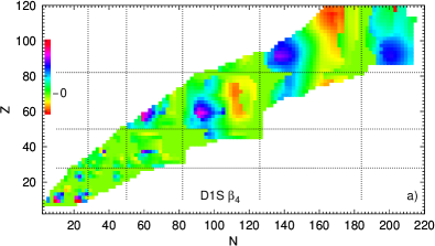
Figure 1: (Color online) Color map of the ground state hexadecapole deformation obtained with the HFB method and the Gogny D1S force. The color scale ranges from $\beta_{4}=-0.2$ up to $\beta_{4}=0.5$ with $\beta_{4}=0$ corresponding to green.

Since the wave functions $|{\varphi}(\bm{\beta})\rangle$ do not form an orthonormal set, the $f_{\sigma}^{\pi}(\bm{\beta})$ are not probability amplitudes. One can define genuine probabilities by folding them with a square root of the norm ${\cal{N}}^{\frac{1}{2}}$ kernel

$$G_{\sigma}^{\pi}(\bm{\beta})=\int d\bm{\beta}{\cal{N}}^{\frac{1}{2}}(\bm{\beta},\bm{\beta}^{\prime})f_{\sigma}^{\pi}(\bm{\beta}^{\prime})$$ (5)

See, Refs. [19] for details on how to solve the GHW equation and how to interpret its solution.

As it is customary in this type of calculations the integrals over the continuous $\beta_{2}$ and $\beta_{4}$ variables are discretised in a mesh with step sizes $\Delta\beta_{2}=0.02$ and $\Delta\beta_{4}=0.02$. The intervals considered are $[-0.4,0.8]$ for $\beta_{2}$ and $[-0.4,0.6]$ for $\beta_{4}$. We have checked that reducing the number of point in each direction to half the nominal value has a negligible impact on the results.

For the calculations presented in this study we have used two sets of parametrizations of the Gogny force. One is the traditional D1S parametrization [20] which has been used for more than forty years to describe many nuclear properties all over the Segrè chart. The other one is the recently proposed D1M* [21] parametrization which is a variation of D1M [22] retaining most of its properties but improving on the description of neutron stars by imposing a different value of the slope of the symmetry energy [23].

III Results and discussions

Results obtained for two isotopic chains in the rare earth region are discussed in this section. The nuclei considered are those of Sm ($Z=62$) and Gd ($Z=64$) and the choice is guided by the results of systematic HFB calculations with the Gogny D1S force. In Fig. 1 the ground state $\beta_{4}$ deformation parameter obtained for a large set of even-even nuclei is depicted as a color map. The ground state $\beta_{4}$ values in the figure range from $\beta_{4}=-0.1$ up to $\beta_{4}=0.3$. One observes that a large fraction of nuclei show zero hexadecapole deformation in their ground state. The largest positive values are obtained in the lower $Z$ sector of rare earth (actinide) with proton numbers 60 (90) and neutron numbers 90 (136), a few units above magic numbers. On the other hand, the largest negative values are also located in the same regions but this time in the upper $Z$ sector with values around 72 (118) and neutron numbers around 110 (170) which are a few units below magic numbers. There are two additional regions with large positive $\beta_{4}$ values at the proton drip line with $Z=60$ and close to the neutron drip line at $Z=90$ and $N=200$. The regions of positive and negative $\beta_{4}$ values are consistent with the polar-gap model of Ref. [24] developed to understand $\beta_{4}$ deformation parameters in the rare earth nuclei [25]. In the model, positive (negative) $\beta_{4}$ values appear at the beginning (end) of the shell.

The figure points to very large positive $\beta_{4}$ deformation parameters in the region under study with N around 90 and Z around 60. For the nucleus ¹⁵⁴Sm considered below a ground state hexadecapole deformation $\beta_{4}=0.21$ is obtained. The $\beta_{4}$ deformation parameter is obtained with Eq. (1) and may differ from other deformation parameters defined, for instance, in terms of $\langle r^{4}\rangle$ instead of $R_{0}^{4}$. Those tend to be smaller, and in the case of ¹⁵⁴Sm one gets $\beta_{4}=0.17$ instead of $\beta_{4}=0.21$ obtained with Eq. (1).

Finally, let us mention that our results for $\beta_{4}$ are consistent in absolute value with those of a recent Skyrme interaction BSkG1 [3]. However, both our results and the ones in [3] tend to be larger than the ones obtained with mic-mac models [2]. For instance, for ¹⁵⁴Sm Moller et al obtain $\beta_{4}=0.11$. The source for the discrepancy could be associated to the different definition of the $\beta_{l}$ parameters as discussed above.

In a recent publication [26] very large values of both $\beta_{2}$ and $\beta_{4}$ have been obtained in inelastic proton scattering experiments in inverse kinematics on the rare isotopes ⁷⁴Kr and ⁷⁶Kr. For ⁷⁶Kr one obtains $\beta_{2}=0.40$ and $\beta_{4}=0.201$ whereas for ⁷⁴Kr one obtains $\beta_{2}=0.35$ and $\beta_{4}=0.23$. Those findings do not agree with the results obtained with Gogny D1S (see Fig. 1 above and Ref. [1]) that seem to favor spherical or nearly spherical ground states for those two isotopes. The discrepancy could possibly be resolved by taking into account that the Kr isotopes represent one of the most prominent examples of shape coexistence with very flat potential energy surfaces and large fluctuations along the quadrupole degree of freedom. This is the realm where the theoretical techniques used in this paper are most relevant and therefore the present calculations are being extended to the Kr region and will be reported in the future.

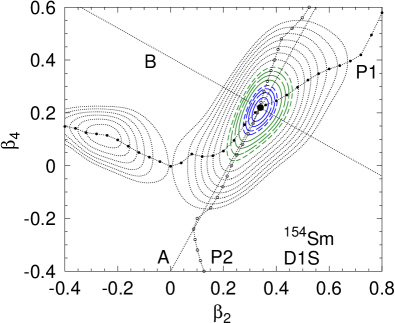
Figure 2: (Color online) Contour plot of the HFB energy as a function of $\beta_{2}$ (horizontal axis) and $\beta_{4}$ (vertical axis). The position of the absolute minimum is indicated by a large dot. The lowest four contours (blue) correspond to energies $E_{min}+\delta En$ with $\delta E=0.25$ MeV. The next four (green) correspond to energies $E_{min}+1\textrm{MeV}+\delta En$ with $\delta E=0.5$ MeV. The remaining contours, starting at $E_{min}+4\textrm{MeV}$ are separated by 1 MeV. The filled (empty) dots connected by a curve correspond to the self-consistent values of $\beta_{4}$ ($\beta_{2}$) obtained in the 1D calculation as a function of $\beta_{2}$ ($\beta_{4}$). The paths are labeled P1 and P2, respectively. The two perpendicular dotted lines crossing at the minimum are drawn along the two principal axes (A and B) of the parabola that approximates the HFB energy around the minimum.

Figure 3: (Color online) In panel a) the potential energy surface as a function of $\beta_{2}$ is drawn for the nucleus ¹⁵⁴Sm along the path P1 of Fig. 2. The three dots correspond to the three lowest solutions of the 1D GCM and are plotted at the corresponding energies and average $\beta_{2}$ values. In panel b) the self-consistent $\beta_{4}$ deformation is plotted as a function of $\beta_{2}$. Finally, in panel c) the collective amplitudes of the GCM $g_{\sigma}(\beta_{2})$ are plotted for the lowest three solutions of the GCM. The curves are shifted by the excitation energy of the corresponding states (y-axis).

III.1 The nucleus ¹⁵⁴Sm

Figure 4: (Color online) Same as Fig. 3 but for the path B shown in Fig. 2.

In this section we discuss at length all the details and peculiarities of our methodology in the paradigmatic case of ¹⁵⁴Sm. The HFB energy corresponding to the nucleus ¹⁵⁴Sm obtained with the D1S parametrization of the Gogny force is shown in Fig. 2. The energy shows a parabolic behavior around the minimum (marked by a large dot) with principal axes going in directions not parallel to the horizontal and vertical axes. This fact implies that in this case $\beta_{4}$ changes substantially when one moves along the bottom of the energy valley as a function of $\beta_{2}$. In a more quantitative way we can say that the hexadecapole deformation corresponding to the bottom of the energy valley shows an approximate linear relation $\beta_{4}=1.8\beta_{2}-0.4$ as a function of $\beta_{2}$. This direction in the $\beta_{2}-\beta_{4}$ plane is denoted as A. The perpendicular direction, denoted by B, will be discussed below. The linear behavior implies that a GCM calculation using as generating parameter the $\beta_{4}$ deformation alone (path P2 in the figure) will explore roughly the same configuration around the energy minimum as a GCM calculation with the $\beta_{2}$ deformation alone (path P1). Therefore, except on those situations where the bottom of the valley runs parallel to either $\beta_{2}$ or $\beta_{4}$ axis the quadrupole and hexadecapole degrees of freedom cannot be decoupled and the full fledged two dimensional GCM has to be considered. In contrast, $\beta_{3}$ usually decouple from $\beta_{2}$ when the two degrees of freedom are considered together [18]. As discussed below, an alternative to the 2D calculation could be the use of collective variables along A and B directions.

For the valley in the oblate side one has $\beta_{4}\approx-0.37\beta_{2}$ and an energy exceeding 4 MeV the one of the prolate side. This energy difference between both minima implies that the oblate minimum is not playing an active role except for high lying excited states.

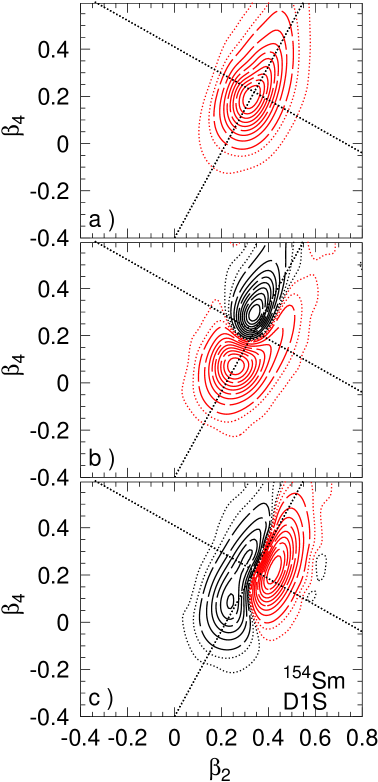
Figure 5: (Color online) Contour plot of the collective amplitudes $g_{\sigma}(\beta_{2},\beta_{4})$ as a function of $\beta_{2}$ (horizontal axis) and $\beta_{4}$ (vertical axis) for the three lowest stated obtained in the 2D GCM. Black (red) contours correspond to positive (negative) values of $g_{\sigma}$. Contours (dashed) correspond to 90 %, 80 %, $\ldots$ of the maximum value of $g_{\sigma}$ except the last two (dotted) that are drawn at 5% and 1% of the maximum value. The perpendicular straight lines are the same drawn in the HFB energy case in Fig. 2.

The results of the calculation just considering $\beta_{2}$ as collective coordinate (path P1 in Fig. 2) are shown in the three panels of Fig. 3. In Fig. 3(a) the HFB energy as a function of $\beta_{2}$ is shown. Two minima, one prolate and the other oblate are found, with the deeper prolate one the ground state. The oblate minimum has little influence in this case as it lies high up in energy as compared to the ground state. The $\beta_{4}$ deformation parameter is shown in Fig. 3(b). The deformation parameter decreases almost linearly for negative $\beta_{2}$ reaching a value close to zero at $\beta_{2}=0$. From there on, a linear increase is observed. The ground state at $\beta_{4}=0.21$ is rather large as compared to other regions of the nuclear chart. In Fig. 3(c) the collective wave function $g_{\sigma}(\beta_{2})$ obtained in the 1D GCM is shown for the three lowest states. The wave functions are situated with respect to the $y$ axis according to the corresponding excitation energy of the collective state. Typical shapes, similar to the ones of the lowest states of the 1D harmonic oscillator (HO), are seen for the collective wave functions. The ground state has a Gaussian distribution peaked at the ground-state $\beta_{2}$ deformation. The fist excited state has a node at the $\beta_{2}$ deformation of the ground state and decays like a Gaussian away from the minimum. The next excited state shows two nodes. All the wave functions show some distortions with respect to the ones of the HO. This can be attributed to deviations of collective potential and inertia from the harmonic form . The absolute energy of the three states is plotted in Fig. 3(a) as bullets placed in the $\beta_{2}$ axes according to the average $\beta_{2}$ value of the correlated state. In the present case, the average $\beta_{2}$ value is rather similar for the three states. A similar calculation but using the $\beta_{4}$ deformation as collective coordinate (path P2 inf Fig. 2) shows similar results as will be discussed below. This is not surprising if one compares the paths explored in both calculations and depicted in Fig. 2. As expected [28] (Chapter 7) the paths do not coincide with the bottom of the 2D valley due to the fact that in the 1D calculations the minimum of the energy is obtained subject to the corresponding constraint, i.e. along vertical (horizontal) lines in the $\beta_{2}$ ($\beta_{4}$) potential energy surface (which is the quantity shown in Fig. 2). However, the two paths are rather close to each other in the region close to the minimum and, as a consequence, the dynamics is rather similar in the two 1D GCM calculations.

Table 1: Results of GCM calculations for ¹⁵⁴Sm. First column labels the type of calculation, either a 1D ($\beta_{2}$ along path P1 or $\beta_{4}$ along path P2) or 2D ($\beta_{2}-\beta_{4}$). The upper (last) three rows correspond to the results obtained with D1S (D1M*) parametrization of the Gogny force. The remaining columns are divided into sets of three. The first set shows the correlation energy and the two moments $\beta_{2}$ and $\beta_{4}$ of the density distribution. The other two sets show excitation energies and corresponding moments.

	$E_{c}$	$\beta_{2}$	$\beta_{4}$	$E_{1}$	$\beta_{2}$	$\beta_{4}$	$E_{2}$	$\beta_{2}$	$\beta_{4}$
$\beta_{2}$ (P1)	0.694	0.33	0.19	2.576	0.27	0.13	3.827	0.37	0.21
$\beta_{4}$ (P2)	0.663	0.33	0.21	2.407	0.30	0.16	4.230	0.28	0.11
$\beta_{2}-\beta_{4}$	1.239	0.33	0.21	2.635	0.30	0.17	3.059	0.37	0.20
$\beta_{2}$ (P1)	0.637	0.32	0.18	2.933	0.29	0.14	4.261	-0.23	0.10
$\beta_{4}$ (P2)	0.707	0.32	0.19	2.447	0.28	0.12	4.615	0.28	0.12
$\beta_{2}-\beta_{4}$	1.305	0.32	0.19	2.685	0.27	0.13	3.210	0.37	0.22

At this point it is worth to discuss the results of another 1D calculation, this time along the line marked as B in Fig. 2 and perpendicular to the bottom of the energy valley. In order to carry out the calculation a set of HFB states was generated with $\beta_{2}$ in the range $[0.1,0.6]$ and $\beta_{4}$ constrained to be in the $\beta_{4}=-0.56\beta_{2}+0.41$ line. The results obtained are summarized in Fig. 4. In panel (a) the HFB energy shows a well defined and deep quadratic well. In panel (b) the $\beta_{4}$ deformation follows a straight line as it should be. Finally, in panel (c) the collective wave functions are shown. They follow closely the expectations for a pure harmonic oscillator. The correlation energy gained by the ground state in this 1D GCM calculation is 0.555 MeV. The excitation energy of the lowest excited state is 3.075 MeV and at roughly twice the excitation energy, 6.509 MeV, the second phonon state is located.

Coming back to the two dimensional (2D) calculation, it is interesting to analyze the behavior of the collective wave function $g_{\sigma}(\beta_{2},\beta_{4})$ solution to the Hill-Wheeler-Griffin equation. The quantities, corresponding to the three lowest solutions are shown in Fig. 5. The upper panel (a) corresponds to the ground state and shows the typical 2D Gaussian shape but tilted with respect to the $\beta_{2}$ and $\beta_{4}$ axes and closely aligned with respect to the A and B directions, shown as perpendicular dotted lines in the plot. The A and B directions run along the bottom of the energy valley (A) and the perpendicular direction (B). The middle panel (b) is for the first excited state. The shape corresponds to a Gaussian along the B principal axis. Along the direction of the principal axis A the shape of the wave function corresponds to a one-phonon state in a 1D HO. By comparing with the collective wave functions of Fig. 3 we conclude that this state corresponds to a collective phonon in which the quadrupole and hexadecapole degrees of freedom are mixed together. Finally, the last panel (c) corresponds to the second excited state that can be interpreted as a 1D phonon along the B direction. We conclude from the present analysis that both quadrupole and hexadecapole degrees of freedom are strongly interleaved and it is better to talk about the A and B directions (or degrees of freedom) instead. It is interesting to note that A and B are given by linear relations (see above) in terms of $\beta_{2}$ and $\beta_{4}$ at least locally around the HFB minimum.

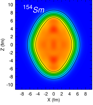
Figure 6: (Color online) The matter density distribution of the mean field ground state of ¹⁵⁴Sm is shown. The mean field deformation parameters (Eq. 1) for this state are $\beta_{2}=0.32$ and $\beta_{4}=0.21$

In Table 1 we show several quantities obtained in the GCM calculation in the 2D and 1D cases with both D1S and D1M* parametrizations of the Gogny force. The correlation energy $E_{c}$ gained in the two 1D calculations for D1S are similar corroborating the conclusion previously drawn about the equivalence of the 1D GCM results irrespective of the use of the $\beta_{2}$ and $\beta_{4}$ collective coordinates (paths P1 and P2). The 2D correlation energy is, accidentally, twice as large as the 1D one with a significant energy gain of 0.6 MeV due to the inclusion of the hexadecapole degree of freedom. This quantity is not negligible and its evolution with proton and neutron number could have significant impact on the reproduction of experimental binding energies. In this respect, modern energy density functionals (EDFs) are able to reach a root mean square (rms) deviation for the binding energies of around 700 keV [22, 29]. For a systematic study of octupole correlation energies the reader is referred to Ref. [30]. It is also important to note that the 2D correlation energy is consistently given as the sum of the quantity obtained in the 1D calculation along path P1 plus the correlation energy obtained along path B. In this example as well as in the other nuclei considered below the additional correlation energy gained in going from the 1D to the 2D case is similar to the one of the quadrupole dynamics alone indicating a very slow convergence of the correlation energy with the (even) multipole degrees considered in the GCM. Whether this is a feature of this specific region or a general trend should be analyzed by extending this type of calculation to a significantly wider sample of nuclei in the nuclear chart. It is to be expected that correlation energy corresponding to multipoles of order six or higher should be significantly smaller than the one of lower multipole orders and the general argument was given in the introduction. This is, however, a still to be answered question that deserves further consideration.

The deformation parameters of the ground and first excited states do not change much in going from the 1D to the 2D GCM results. It is also remarkable that the ground state $\beta_{2}$ and $\beta_{4}$ GCM values are similar to the ones obtained at the HFB level. This result is not surprising as the ground state collective wave function is centered at the position of the HFB minimum. However, the deformation parameters change significantly for the second excited states with respect to the ground state values. Regarding the excitation energies, the first excited state behaves similarly in the 1D and 2D calculations, but this is not the case for the second state. It is easy to understand the origin of the difference by looking at Fig. 5: the second excited state is a 1D phonon along path B, not present by definition in the 1D case. It is worth to remember that this state is the first excited state in the 1D calculation along path B discussed previously. Its excitation energy is slightly above 3 MeV and therefore could be one of the many $0^{+}$ excited states found in many nuclei in the region. However, the value of the excitation energy is perhaps a bit too high and therefore its features would be difficult to characterize experimentally.

As a side comment, it is remarkable the mild dependence of the results with the parametrization of the Gogny force used. Both share the same functional form, but the parameters were adjusted with rather different targets in mind. For instance, D1M^∗ produces much better quality binding energies than D1S and it is also expected to behave better in the neutron rich sector.

A comparison with the experimental data [31] for the lowest excited $0^{+}$ states reveals a discrepancy of more than a factor of two between theory and experiment being the experimental data smaller than the theoretical predictions. In the ¹⁵⁴Sm nucleus there are a couple of known excited $0^{+}$ at excitation energies slightly above 1 MeV. However, it is not clear whether those two states can be unambiguously identified with a genuine $\beta$ vibration as discussed in [32, 33]. In these references, it is argued that $\beta$ vibrations should lie higher in energy due to the kind of excitations involved and its excitation energy very sensitive to pairing effects, not taken explicitly into account in the present description. On the other hand, the theoretical description includes a limited set of collective degrees of freedom and it is very likely that triaxial and pairing effects can play a role in the properties of the first excited state. One also should not forget that the GCM formalism do not take into account collective momentum degrees of freedom. The impact of those on the dynamics is not well studied but based on the large differences between collective inertias for fission obtained with the Adiabatic Time Dependent (ATD) and the GCM frameworks [34] an important reduction of the excitation energies consequence of the use of collective momentum degrees of freedom is to be expected. There is additional insight pointing to this effect coming from Random Phase Approximation results [35]. As a conclusion, all the above effects should be considered to have a more precise estimation of the hexadecapole $K=0^{+}$ vibrational excitation energy. It is likely that its value will be lower than the present prediction and therefore more likely to be characterized experimentally.

The quadrupole deformation parameter is larger than the one in [36] and also in [2] but the difference could be attributed to the definition of $\beta_{2}$. If one uses the definition of $\beta_{2}$ with $\langle r^{2}\rangle$ instead of $3/5R^{2}$ with $R=r_{0}A^{1/3}$ used here, smaller values are obtained (typically 20 % smaller ). The same also holds true for $\beta_{4}$ but in this case the deviation of the present results with respect to the ones of Refs. [36, 2] is as large as a factor of two. A comparison with experimental data of Refs. [37, 38] also indicates an overestimation of $\beta_{4}$ with respect to the experiment by a factor of 2.

As the deformation parameters for ¹⁵⁴Sm and all the studied nuclei considered in this paper (see below) are rather large, larger than the ones predicted by Moller in [2], it is therefore instructive to have a look at the spatial distribution of the matter density for the HFB solution at the minimum shown in Fig. 6. One observes the typical diamond like shape characteristic of positive $\beta_{4}$ values.

III.2 Potential energy surfaces of Gd and Sm

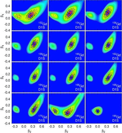
Figure 7: (Color online) Potential energy surfaces as a function of $\beta_{2}$ and $\beta_{4}$ deformation parameters for the Gd isotopes considered. The results are obtained with Gogny D1S.

The HFB energy as a function of $\beta_{2}$ and $\beta_{4}$ for the nuclei in the isotopic chain of Gd is shown in Fig. 7. Most of the energies show a valley whose bottom roughly follows a straight line with positive slope in the $\beta_{2}-\beta_{4}$ plane for prolate deformations. The valley bends at $\beta_{2}\approx 0$ to acquire a negative slope but the excitation energy in that region is large and its effect on the ground state low energy dynamic can be disregarded. The only two exceptions are the isotope of ¹⁸⁰Gd where the oblate minimum lies quite low in energy and the isotope of ¹⁹⁰Gd with magic neutron number $N=126$ which shows the characteristic behavior of a spherical nucleus. The ground state minimum takes place at rather large $\beta_{4}$ values and all of them are prolate deformed. For the Sm isotopes to be discussed later on, the results look very similar and therefore are not shown here. The HFB energy looks rather similar to the ¹⁵⁴Sm one discussed in the previous section and therefore all the considerations there apply to all the nuclei in the chain exception made of ¹⁸⁰Gd where prolate and oblate minima coexist and ¹⁹⁰Gd which is a semi-magic spherical nucleus.

III.3 Generator coordinate method results for Gd and Sm

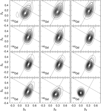
Figure 8: (Color online) Contour plots of the collective ground state wave function $g_{0}(\beta_{2},\beta_{4})$ of Eq. (5) obtained by solving the GHW equation in the Gd isotopes. The results are obtained with Gogny D1S.

In Fig. 8 the collective amplitude corresponding to the ground state is shown for the considered nuclei. Following the discussion of the ¹⁵⁴Sm case, one clearly identify the characteristic two dimensional Gaussian shape with principal axes aligned roughly in the same directions A and B s in the ¹⁵⁴Sm case.

In Fig. 9 the collective amplitude corresponding to the first excited state is shown for the considered nuclei. Following the discussion of the ¹⁵⁴Sm case, one clearly identify the characteristic two dimensional shape corresponding to a 1D phonon in the collective variable along the bottom of the valley (path A). In the ¹⁸⁰Gd case, the first excited state corresponds to a shape coexisting oblate configuration and the collective amplitude is concentrated in the oblate minimum. In the ¹⁹⁰Gd magic nucleus, the first excited state is a pure $\beta_{2}$ vibration.

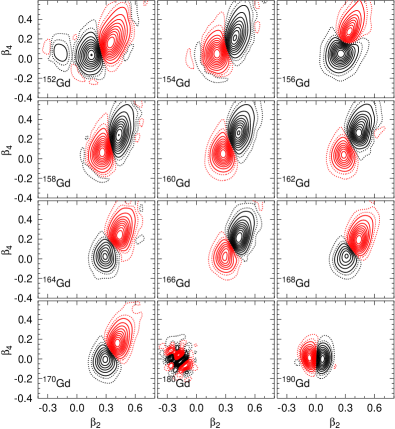
Figure 9: (Color online) Contour plots of the collective first excited state wave function $g_{1}(\beta_{2},\beta_{4})$ of Eq. (5) obtained by solving the GHW equation in the Gd isotopes. Black (red) contour lines correspond to positive (negative) values of the collective wave function $g_{1}(\beta_{2},\beta_{4})$. The results are obtained with Gogny D1S.

In Table 2 the results obtained for the ground state and two first excited states in the 2D $\beta_{2}-\beta_{4}$ calculations are given as a function of mass number $A$ for the Gd isotopes. In the second column the correlation energy gained by the collective motion $\beta_{2}-\beta_{4}$ on top of the mean field ground state energy is given. Overall, one observes a gain of around 1.2 MeV correlation energy, but the behavior as a function of $A$ is not constant with a minimum of 0.99 MeV for $A=164$ and a maximum of 1.46 MeV for $A=154$. The additional 600 keV binding energy gain associated with the hexadecapole degree of freedom can be important for a proper description of binding energies with the accuracy required by modern applications [22, 29]. In the third and fourth columns the $\beta_{2}$ and $\beta_{4}$ deformation parameters are given, Our $\beta_{2}$ parameters are typically 25% larger than the ones given by Moller [2] and the only isotope where they agree is the spherical ¹⁹⁰Gd. On the other hand, our $\beta_{4}$ values are a factor of two larger. The GCM ground state deformation parameters are similar to the ones obtained at the mean field level. In the next three columns, the excitation energy of the first excited state $0^{+}$ (phonon along the A direction) along with its $\beta_{2}$ and $\beta_{4}$ deformation parameters are given. The excitation energy ranges from 0.6 to 3.7 MeV depending on the isotope and both deformation parameters are slightly larger than those of the ground state. In ¹⁸⁰Gd, the first excited $0^{+}$ is oblate and lies at a quite low excitation energy of 612 keV with a $\beta_{2}=-0.19$ and zero hexadecapole deformation. The Gd isotopes with A=152 and 154 show prolate-oblate shape coexistence that manifest in a different structure of the collective wave function of the first excited state (see Fig. 9). As a consequence, the excitation energy of the first excited state is relatively low with values of 1.5 and 1.9 MeV, respectively. The same holds true for the isotopes with A=168 and 170 but with a less pronounced prolate-oblate mixing. For the intermediate isotopes, without shape coexistence the energy goes up to around 3.5 MeV. For the second excited $0^{+}$ the excitation energies follow the same pattern as for the first excited state associated to the existence of prolate-oblate shape coexistence. For mass numbers around 162 it goes up to around 4.8 MeV. Interestingly, the $\beta_{2}$ deformation of the second excited state becomes negative for A=152, 154 and 170 as a clear manifestation of prolate-oblate mixing. All the remaining isotopes have similar deformation parameters as the ground state. The excitation energy of the second excited state (phonon along B direction) appears too high except in those cases where prolate-oblate shape coexistence is present. As discussed in the previous subsection in the ¹⁵⁴Sm case, some missing degrees of freedom might reduce the excitation energy a bit. Using the typical reduction of a factor 0.7 consequence of considering ATD versus GCM inertias (a simple way to take into account momentum-like collective coordinates) one could expect excitation energies for the phonon along B direction to come down to 3-3.5 MeV which is perhaps too high to be characterized experimentally. For those cases where prolate-oblate shape coexistence is present the above reduction factor will bring the excitation energy to a quite low value but the price to pay would be to disentangle the impact of shape coexistence in the characteristics of the vibrational state.

Table 2: Same as Table 1 but for the 2D GCM calculation of all the Gd isotopes considered and using the D1S parametrization of the force.

A	$E_{c}$	$\beta_{2}$	$\beta_{4}$	$E_{1}$	$\beta_{2}$	$\beta_{4}$	$E_{2}$	$\beta_{2}$	$\beta_{4}$
152	1.384	0.23	0.10	1.547	0.27	0.13	1.638	-0.16	0.06
154	1.464	0.30	0.16	1.874	0.29	0.13	2.790	-0.21	0.08
156	1.325	0.33	0.18	2.631	0.29	0.14	2.836	0.38	0.20
158	1.290	0.34	0.17	3.191	0.35	0.16	3.876	0.35	0.15
160	1.148	0.35	0.15	3.502	0.36	0.16	4.422	0.38	0.14
162	1.153	0.35	0.13	3.710	0.39	0.20	4.836	0.38	0.14
164	0.991	0.36	0.11	3.665	0.41	0.21	4.830	0.35	0.11
166	1.028	0.36	0.09	3.114	0.41	0.18	3.854	0.37	0.10
168	1.141	0.35	0.07	2.217	0.42	0.17	4.514	0.36	0.09
170	1.233	0.34	0.05	1.887	0.39	0.12	4.161	-0.25	0.06
180	1.491	0.23	-0.05	0.612	-0.19	0.00	1.776	0.30	0.01
190	1.196	0.00	0.00	3.987	-0.00	0.00	5.735	-0.00	0.01

In Table 3 the results obtained for the Sm isotopic chain are presented. The features of the ground, first and second excited states are very similar to the ones of the corresponding Gd isotopes with the same mass number plus two. It becomes apparent that a change of two units in proton number is not changing in a relevant way the Gd results except in very specific situations like the $\beta_{2}$ deformation of the second excited state in ¹⁵²Sm. These specific cases can be traced back to a subtle interplay of the collective wave functions associated to prolate-oblate shape coexistence in those systems.

Table 3: Same as Table 1 but for the 2D GCM calculation of all the Sm isotopes considered and using the D1S parametrization of the force.

A	$E_{c}$	$\beta_{2}$	$\beta_{4}$	$E_{1}$	$\beta_{2}$	$\beta_{4}$	$E_{2}$	$\beta_{2}$	$\beta_{4}$
150	1.338	0.23	0.10	1.496	0.28	0.14	1.996	-0.16	0.06
152	1.403	0.31	0.18	1.879	0.28	0.12	3.076	0.31	0.17
154	1.239	0.33	0.21	2.635	0.30	0.17	3.059	0.37	0.20
156	1.174	0.35	0.20	3.319	0.33	0.15	4.083	0.36	0.17
158	1.072	0.35	0.18	3.464	0.34	0.16	4.629	0.39	0.16
160	0.968	0.36	0.15	3.554	0.37	0.19	4.943	0.40	0.16
162	0.961	0.36	0.13	3.390	0.39	0.20	4.845	0.36	0.14
164	1.046	0.36	0.11	2.725	0.40	0.18	4.233	0.36	0.11
166	1.194	0.36	0.10	1.648	0.41	0.16	4.172	0.35	0.09
168	1.371	0.35	0.09	1.452	0.37	0.11	3.951	-0.26	0.07

IV Summary

Systematic HFB calculations with the Gogny D1S force show several regions of the nuclear chart where the ground state hexadecapole deformation is non zero. In this paper the region corresponding with $Z=62$ and 64 (Sm and Gd) and positive $\beta_{4}$ values is studied with the GCM method for the $K=0^{+}$ quadrupole and hexadecapole degrees of freedom. The gain in binding energy due to those correlations is computed as well as the position of the first and second $0^{+}$ states corresponding to vibrational states along collective degrees of freedom where quadrupole and hexadecapole are strongly interleaved. For some of the isotopes considered prolate-oblate shape coexistence impacts excitation energies and deformation parameters of excited states in a substantial way. For the more pure vibrational states showing up in some other isotopes excitation energies come up too high to be amenable to an easy experimental characterization. A discussion of relevant missing degrees of freedom that could reduce the excitation energies is presented. We conclude that the physics brought by considering the hexadecapole degree of freedom is not trivial and its study is worth further consideration. In a forthcoming publication we plan to extend the present analysis to nuclei in the rare earth region with negative $\beta_{4}$ values in their ground states.