Generative Forests
Abstract
Tabular data represents one of the most prevalent form of data. When it comes to data generation, many approaches would learn a density for the data generation process, but would not necessarily end up with a sampler, even less so being exact with respect to the underlying density. A second issue is on models: while complex modeling based on neural nets thrives in image or text generation (etc.), less is known for powerful generative models on tabular data. A third problem is the visible chasm on tabular data between training algorithms for supervised learning with remarkable properties (e.g. boosting), and a comparative lack of guarantees when it comes to data generation. In this paper, we tackle the three problems, introducing new tree-based generative models convenient for density modeling and tabular data generation that improve on modeling capabilities of recent proposals, and a training algorithm which simplifies the training setting of previous approaches and displays boosting-compliant convergence. This algorithm has the convenient property to rely on a supervised training scheme that can be implemented by a few tweaks to the most popular induction scheme for decision tree induction with two classes. Experiments are provided on missing data imputation and comparing generated data to real data, displaying the quality of the results obtained by our approach, in particular against state of the art.
1 Introduction
There is a substantial resurgence of interest in the ML community around tabular data, not just because it is still one of the most prominent kind of data available [5]: it remains one of the last data bastions that still resists deep learning and its arsenal of neural architectures [13], still not on full par with traditional, tree-based methods. In the field of data generation, there has been an early push to develop neural nets for tabular data [41] (and references therein). In parallel, there has been a rich literature on models to represent densities directly applicable to tabular data [4, 6, 27, 32, 29, 31] (and many others). Generating data from an explicit density can be tricky, even more when it comes with the constraint to be exact with respect to the density [35]. A few recent papers have explored models leading to both the density and a simple exact sampler [23, 38]. In [23], models are simple trees and very strong convergence guarantees are obtained in the boosting model. In [38] models are a convex combination of tree generators called adversarial random forests. Convergence in the limit are obtained but with very restrictive assumptions on the target density. Also, relying on a convex combination of trees makes it necessary to learn fairly complex trees to model realistic or tricky densities. Both [23, 38] are based on the adversarial training setting of GANs and thus involve training generators and a discriminators [10].
| domain | 1 tree, 50 splits | 50 stumps |
![[Uncaptioned image]](/html/2308.03648/assets/x1.png) |
![[Uncaptioned image]](/html/2308.03648/assets/x2.png) |
![[Uncaptioned image]](/html/2308.03648/assets/x3.png) |
In this paper, we first introduce new generative models based on sets of trees that we denote as generative forests (gf). When there is one tree in the ensemble, it operates like a generative tree of [23]. With more than one tree in the ensemble, the model bring a sizeable combinatorial advantage over both generative trees [23] (see Table 1 for an example) and also adversarial random forests [38]. We also show how to get rid of the adversarial training setting of [23, 38] to train just the generator, furthermore without the need to generate data during training. This algorithm, that we call gf.Boost, can be implemented by a few tweaks on the popular induction scheme for decision tree induction with two classes, which paves a simple way for code reuse to learn powerful generative models from the huge number of repositories / ML software implementing algorithms like CART or C4.5 [26, 3, 39]. Most importantly, we show that gf.Boost is a boosting algorithm under a weak learning assumption which parallels that of supervised learning [34]. Finally, we introduce a second new class of tree-based generative models with a memory footprint much smaller than for gf but keeping their combinatorial properties, that we call ensembles of generative trees (eogt) and provide a way to generate observations with guaranteed approximation to the generative forest with the same trees. Experimentally, we mainly focus on two problems, missing data imputation and assessing the realism of generated data, demonstrating that our models can be competitive with or substantially beat the state of the art (respectively mice [37] for missing data imputation and adversarial random forests [38] and CT-GANs [41] for the realism of generated data) on a wide range of domains. Our experiments also demonstrate that the observation of Table 1 can hold even for real-world domains as a small number of small trees (even stumps) in a generator can be enough to get state of the art results. All proofs, additional experiments and a few additional results are given in an Appendix.
2 Related work
| density | sampler | training | ||||||
| ref. | base model | any feat. | explicit | handles missing | ? | density | handles missing | conv. rates |
| [10, 16] | Deep Net | ✓ | ✗ | ✗ | ✓ | ✓ | ✗ | ✓ |
| [4, 6, 27, 32] | Graph | ✓ | ✓ | ✓ | ✗ | N/A | N/A | N/A |
| [11] | Deep Net | ✓ | ✓ | ✗ | ✓ | ✗ | ✗ | ✗ |
| [29, 31] | Tree | ✗ | ✓ | ✗ | ✗ | N/A | N/A | N/A |
| [38] | Forest | ✗ | ✓ | ✗ | ✓ | ✓ | ✗ | ✗ |
| [23] | Tree | ✓ | ✓ | ✓ | ✓ | ✓ | ✓ | ✓ |
| This paper | Forest | ✓ | ✓ | ✓ | ✓ | ✓ | ✓ | ✓ |
Related work on generative approaches can be segmented according to two main criteria: the nature of data and what is meant by ”generative”. Alongside data, the most obvious split is between data used for deep learning and data used for tabular models. This split comes from the difference between traditional models used, showing a clear divide [13]. A key difference between deep models and tabular (tree- or graph-based) models is that the former progressively leverage a natural topological dependence among description features (such as pixels in an image, words in a text, etc.), while the latter rely on probabilistic dependences between features, disregarding the natural topological component. Regarding what is meant by ”generative”, many work define it as learning a density (function) modeling a data generation process [4, 6, 27, 29]. This does not entail getting a sampler for the density learned. Of course, standard approaches exist to sample from an analytical density [11], but they usually come with only approximation guarantees to the underlying density and they can be tricky to adapt [35]. In our setting, ”generative” means being able to get both a density and a sampler that exactly follows the underlying density. Table 2 summarizes key approaches.
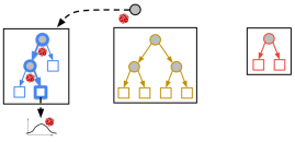
The closest approaches to ours are [38] and [23], first and foremost because the models include trees with a stochastic activation of edges to pick leaves, and a leaf-dependent data generation process. While [23] learn a single tree, [38] use a way to generate data from a set of trees – called an adversarial random forest – which is simple: sample a tree, and then sample an observation from the tree. Hence, the distribution is a convex combination of the trees’ density. This is simple but it suffers several drawbacks: (i) each tree has to be accurate enough and thus big enough to model ”tricky” data for tree-based models (tricky can be low-dimensional, see the 2D data of Figure 1); (ii) if leaves’ samplers are simple, which is the case for [23] and our approach, it makes it tricky to learn sets of simple models, such as when trees are stumps (we do not have this issue, see Figure 1). In our case, while our models include sets of trees, generating one observation makes use of leaves in all trees instead of just one as in [38]. We note that the primary goal of that latter work is in fact not to generate data [38, Section 4]. In general, theoretical results that are relevant to data generation are scarce (we restrict ourselves to tabular models, thus omitting the large number of references available for deep nets). In [38], formal convergence results are given but they are relevant to statistical consistency (infinite sample) and they also rely on assumptions that are not realistic for real world domains, such as Lipschitz continuity of the target density, with second derivative continuous, square integrable and monotonic. The assumption made on models, that splitting probabilities on trees is lowerbounded by a constant, is impeding to model real world data.
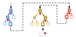
| Adversarial Random Forest [38] | gf/eogt (this paper) |
|
|
In the generative trees of [23], leaf generation is the simplest possible: it is uniform. This requires big trees to model real-world or tricky data. On the algorithms side, [23] introduce two training algorithms in the generative adversarial networks (GAN) framework [10], thus involving the generator to train but also a discriminator, which is a decision tree in [23]. One such algorithm, copycat training, involves copying parts of the discriminator in the generator to speed-up training (also discussed in [12] for neural nets). While strong convergence guarantees are shown in the boosting model, a key limitation of [23] is conceptual: losses have a symmetry property which is not desirable for data generation as it ties the misclassification costs of real and fakes with no argument to do so in general.
3 Definitions
For any integer , we let . Our notations follow [23, 30]. Let denote a binary task, where (and any other measure defined hereafter) are probability measures with the same support, also called domain, , and is a prior. is the corresponding mixture measure. For the sake of simplicity, we assume bounded hereafter, and note that tricks can be used to remove this assumption [23, Remark 3.3]. In tabular data, each of the features can be of various types, including categorical, numerical, etc., and associated to a natural measure (counting, Lebesgue, etc.) so we naturally associate to the product measure, which can thus be of mixed type. We also write , where is the set of values that can take on variable . Several essential measures will be used in this paper, including , the uniform measure, , the measure associated to a generator that we learn, , the empirical measure corresponding to a training sample of observations. Like in [23], we do not investigate generalisation properties.
Loss functions There is a natural problem associated to binary task , that of estimating the probability that an arbitrary observation was sampled from – call such positive – or – call these negative –. To learn a supervised model for such a class probability estimation (cpe) problem, one usually has access to a set of examples where each is a couple (observation, class), the class being in set (=negative, positive). Examples are drawn i.i.d. according to . Learning a model is done by minimizing a loss function: when it comes to cpe, any such cpe loss [2] is some whose expression can be split according to
partial losses , . Its (pointwise) Bayes risk function
is
the best achievable loss
when labels are drawn with a particular positive base-rate,
| (1) |
A fundamental property for a cpe loss is properness which encourages to guess the ground truth. Formally, is proper iff , and strictly proper if . Strict properness implies strict concavity of Bayes risk. For example, the square loss has , , and, since it is strictly proper, Bayes risk . Other popular ML losses are strictly proper, including the log and Matusita’s losses. All these losses are symmetric since [25] and differentiable because both partial losses are differentiable.
In addition to cpe losses, we introduce a set of losses relevant to generative approaches, that are popular in density ratio estimation [22, 36]. For any differentiable and convex , the Bregman divergence with generator is . Given function , the generalized perspective transform of given is , being implicit in notation [20, 21, 24]. The Likelihood ratio risk of with respect to for loss is
| (2) |
with in the generalized perspective transform. Our definition includes the prior multiplication for technical convenience. In addition to being non-negative, a key property of is iff almost everywhere when is strictly proper [23].
4 Generative forests: models and data generation
Architecture
We first introduce the basic building block of our models, trees.
Definition 4.1.
A tree is a binary directed tree whose internal nodes are labeled with an observation variable and arcs are consistently labeled with subsets of their tail node’s variable domain.
Consistency is an important notion, linked to the generative model to which the tree belongs to. We shall define it formally after having introduced our generative models. Informally however, consistency postulates that the arcs’ labels define a partition of the measure’s support via a simple algorithm.
Definition 4.2.
A generative forest (gf), , is a set of trees, , associated to measure .
is implicit in the notation. Figure 2 shows an example of gf. We now proceed to defining the notion of consistency appearing in Definition 4.1. For any node (the whole set of nodes of , including leaves), we denote the support of the node, which is for the root and then is computed as follows otherwise for an internal node : starting with at the root, we progressively update the support as we descend the tree, chopping off a feature’s domain that is not labelling an arc followed, until we reach . Then, a consistent labeling of arcs in a tree complies with one constraint:
-
(C)
for each internal node and its left and right children (respectively), and the measure of with respect to is zero.
Hence, a single tree defines a recursive partition of according to the splits induced by the inner nodes. Such is also the case for a set of trees, where intersections of the supports of tuples of leaves (one for each tree) define the subsets:
| (3) |
Importantly, we can construct the elements of using the same algorithm that would compute it for 1 tree. First, considering a first tree , we compute the support of a leaf, say , using the algorithm described for the consistency property above. Then, we start again with a second tree but replacing the initial by , yielding . Then we repeat with a third tree replacing by , and so on until the last available tree is processed. This yields one element of .
Algorithm 1 Init() Input: Trees of a gf; Step 1 : for ; Algorithm 2 StarUpdate() Input: Tree , subset , measure ; Step 1 : if then ; ; else ; ; Step 2 : if then
| After Init | StarUpdate on | StarUpdate on |
|
|
|
|
| StarUpdate on | StarUpdate on | StarUpdate on |
|
|
|
|
Generating one observation Generating one observation relies on a stochastic version of the procedure just described. It ends up in an element of of positive measure, from which we sample uniformly one observation, and then repeat the process for another observation. To describe the process at length, we make use of two key routines, Init and StarUpdate, see Algorithms 1 and 2. Init initializes ”special” nodes in each tree, that are called star nodes, to the root of each tree (notation for a variable relative to a tree is ). Stochastic activation, performed in StarUpdate, progressively makes star nodes descend in trees. When all star nodes have reached a leaf in their respective tree, an observation is sampled from the intersection of the leaves’ domains (which is an element of ). A Boolean flag, done takes value true when the star node is in the leaf set of the tree ( is Iverson’s bracket for the truth value of a predicate, [17]).
The crux of generation is StarUpdate. This procedure is called with a tree of the gf for which done is false, a subset of the whole domain and measure . The first call of this procedure is done with . When all trees are marked done, has been ”reduced” to some , where the index reminds that this is the last we obtain, from which we sample an observation, uniformly at random in . Step 1 in StarUpdate is fundamental: it relies on tossing an unfair coin (a Bernoulli event noted ), where the head probability is just the mass of in relative to . Hence, if , . There is a simple but important invariant (proof omitted).
Lemma 4.3.
In StarUpdate, it always holds that the input satisfies .
Remark that we have made no comment about the sequence of tree choices over which StarUpdate is called. Let us call admissible such a sequence that ends up with some . being the number of trees (see Init), for any sequence , where is the sum of the depths of all the star leaves whose support intersection is , we say that is admissible for if there exits a sequence of branchings in Step 1 of StarUpdate, whose corresponding sequence of trees follows the indexes in , such that at the end of the sequence all trees are marked done and the last . We note that if we permute two different indexes in , the sequence is still admissible for the same but if we flip an index for another one, it is not admissible anymore for . Crucially, the probability to end up in using StarUpdate, given any of its admissible sequences, is the same and equals its mass with respect to .
Lemma 4.4.
For any and admissible sequence for , .
(Proof in Appendix, Section II.1) The Lemma is simple to prove but fundamental in our context as the way one computes the sequence – and thus the way one picks the trees – does not bias generation: the sequence of tree choices could thus be iterative, randomized, concurrent (e.g. if trees were distributed), etc., this would not change generation’s properties from the standpoint of Lemma 4.4. As a simple example, Algorithm 3 shows how to update the star nodes in an iterative fashion, whose implementation could give the sequence of updates in Figure 1. The Appendix (Section I) shows examples of how to pick the sequence of trees in a distributed / concurrent way or in a purely randomized way, both possibilities being illustrated in a simple case in Figure 3. For any gf and , is the sum of depths of the leaves in each tree whose support intersection is . We also define the expected depth of .
Definition 4.5.
The expected depth of gf is .
represents the expected complexity to sample an observation (see also Lemma 6.2).
5 Learning generative forests: boosting
Algorithm 3 IterativeSupportUpdate() Input: Trees of a gf; Output: sampling support for one observation; Step 1 : ; Step 2 : Init(); Step 3 : for Step 2.1 : while !.done Step 2.1.1 : StarUpdate(); return ; Algorithm 4 gf.Boost(, , ) Input: measure , iters , trees ; Output: trees of gf ; Step 1 : ; Step 2 : for to Step 2.1 : tree (); Step 2.2 : leaf (); Step 2.3 : splitPred ; Step 2.4 : ; return ;
In their paper, [23] show how to train a generative tree with two algorithms in the GAN framework, requiring the help of a discriminator and repeated sampling using the generator. The way we train our generative models provides two improvements to their setting: (i) we do not require sampling the generator during training anymore, and more importantly (ii) we get rid of the discriminator, thus training only the generator. Our training setting is not anymore generative as for GANs, but supervised as our generative models are trained to minimize loss functions for a task called class probability estimation [30], whose key property, properness [33], helped design all decades-old major top-down decision tree induction algorithms [1, 28].
To learn a gf, we just have to learn its set of trees. Our training algorithm, gf.Boost (Algorithm 4), performs a greedy top-down induction. In Step 1, we initialize the set of trees to roots. Step 2.2 picks a candidate leaf to split in the chosen tree and Step 2.4 splits by replacing by a stump whose corresponding splitting predicate, p, is returned in Step 2.3 using a weak splitter oracle called splitPred. ”weak” refers to boosting’s weak/strong learning setting [14] and means that we shall only require lightweight assumptions about this oracle; in decision tree induction, this oracle is the key to boosting from such weak assumptions [15]. This will also be the case for our generative models. Before wrapping up the description of Steps 2.1, 2.2, 2.4, we investigate splitPred.
The weak splitter oracle splitPred
In decision tree induction, a splitting predicate is chosen to reduce an expected Bayes risk (1) (e.g. that of the log loss [28], square loss [1], etc.). In our case, splitPred does about the same with a catch in the binary task it adresses, which is***The prior is chosen by the user: without reasons to do otherwise, a balanced approach suggests .:
| (4) |
The corresponding expected Bayes risk that splitPred seeks to minimize is just:
| (5) |
The concavity of implies . Notation overloads that in (3) by depending explicitly on the set of trees of instead of itself. In classical decision tree induction, (5) is optimized over a single tree: there is thus a single element in which is affected by the split, , which makes the optimization of very efficient from an implementation standpoint. In our case, multiple elements in can be affected by one split, so the optimisation is no more computationally demanding. From the standpoint of the potential decrease of however, a single split in our case can be much more impactful. To see this, remark that for the candidate leaf ,
(because is concave). The leftmost term is the contribution of to , the rightmost its contribution to . In the latter case, the split gets two new terms instead of one, whose expectation is no larger than the contribution of to . In the former case, there can be as much as new contributions, so the inequality can be strict with a substantial slack.
Boosting
Two questions remain: can we quantify the slack in decrease and of course what quality guarantee does it bring for the generative model whose set of trees is learned by gf.Boost ? We answer both questions in a single Theorem, which relies on an assumption that parallels the classical weak learning assumption of boosting (WLA).
Definition 5.1.
(WLA) There exists such that at each iteration of gf.Boost, the couple chosen in Steps 2.2, 2.3 of gf.Boost satisfies the following properties:
-
(a)
is not skinny: ,
-
(b)
the truth values of p moderately correlates with at : ,
-
(c)
and finally there is a minimal proportion of real data at : .
Scrutinising the convergence proof of [15] reveals that both (a) and (b) are jointly made at any split, where our (b) is equivalent to their weak hypothesis assumption where their parameter is twice ours. (c) makes sense with our choice of : the uniform measure of any node with non-empty support is always strictly positive, so we just guarantee that we do not split a node that would be useless for data generation. Our Theorem follows.
Theorem 5.2.
Suppose the loss is strictly proper and differentiable and satisfies for some . Let denote the initial gf with roots in its trees (Step 1, gf.Boost) and the final gf, assuming wlog that the number of boosting iterations is a multiple of . Under WLA, we have the following relationship on the likelihood ratio risks:
As shown in the proof (Appendix, Section II.2), the assumption on is weak in the context of strict properness (e.g. for the square loss). The proof proceeds in two stages, first relating a decrease in Bayes risk (our supervised learning loss) to a decrease of the likelihood ratio risk (our generative loss), and then using a recent result on a general model-adaptive boosting algorithm of [19] to show how their algorithm can emulate gf.Boost, thereby transferring the boosting rate of their algorithm to gf.Boost. Their proof bypasses the symmetry assumption of the loss on which the results of [23] rely. So does our proof and we thus stand on a setting substantially more general than [23] with respect to the losses optimized.
6 Simpler models: ensembles of generative trees
Storing a gf requires keeping information about the empirical measure to compute the branching probability in Step 1 of StarUpdate. This does not require to store the full training sample, but requires at least an index table recording the association, for a storage cost in between and where is the size of the training sample. There is a simple way to get rid of this constraint and approximate the gf by a set of generative trees (gts) of [23].
Models
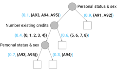
Simply put, a gt is a simplified equivalent representation of a generative forest with 1 tree only. In this case, the branching probabilities in Step 1 of StarUpdate depend only on the tree’s star node position. Thus, instead of recomputing them from scratch each time an observation needs to be generated, we compute them beforehand and use them to label the arcs in addition to the features’ domains, as shown in Figure 4. This representation is equivalent to that of generative trees [23]. If we have several trees, we do this process independently for each tree and end up with an ensemble of generative trees (eogt). The additional memory footprint for storing probabilities () is offset by the fact that we do not have anymore to store associations between leaves and observations for generative forests, for a potentially significant reduction is storing size. However, we cannot use anymore StarUpdate as is for data generation since we cannot compute exactly the probabilities in Step 1. Two questions need to be addressed: is it possible to use an ensemble of generative trees to generate data with good approximation guarantees (and if so, how) and of course how do we train such models.
Data generation
We propose a simple solution based on how well an eogt can approximate a generative forest. It relies on a simple assumption about and . Taking as references the parameters in StarUpdate, we now make two simplifications on notations, first replacing by (tree implicit), and then using notation for any , the reference to the tree / star node being implicit. The assumption is as follows.
Assumption 6.1.
There exists such that at any Step 1 of StarUpdate, for any , we have
| (7) |
A simple condition to ensure the existence of is a requirement weaker than (c) in Definition 5.1: at all Steps 1 of StarUpdate, , which also guarantees and thus postulates that the branching in Step 1 of StarUpdate never reduces to one choice only. The next Lemma shows that it is indeed possible to combine the generation of an ensemble of generative trees with good approximation properties, and provides a simple algorithm to do so, which reduces to running StarUpdate with a specific approximation to branching probabilities in Step 1.
Lemma 6.2.
Note the additional leverage for training and generation that stems from Assumption 6.1, not just in terms of space: computing is and does not necessitate data so the computation of key conditional probabilities (8) drops from to for training and generation in an eogt. Lemma 6.2 (proof in Appendix, Section II.3) provides the change in StarUpdate to generate data.
Training
To train an eogt, we cannot rely on the idea that we can just train a gf and then replace each of its trees by generative trees. To take a concrete example of how this can be a bad idea in the context of missing data imputation, we have observed empirically that a generative forest (gf) can have many trees whose node’s observation variables are the same within the tree. Taken independently of the forest, such trees would only model marginals, but in a gf, sampling is dependent on the other trees and Lemma 4.4 guarantees the global accuracy of the forest. However, if we then replace the gf by an eogt with the same trees and use them for missing data imputation, this results in imputation at the mode of the marginal(s) (exclusively), which is clearly suboptimal. To avoid this, we have to use a specific training for an eogt, and to do this, it is enough to change a key part of training in splitPred, the computation of probabilities used in (5). Suppose very small in Assumption 6.1. To evaluate a split at some leaf, we observe (suppose we have a single tree)
(and the same holds for ). Extending this to multiple trees and any , we get the computation of any and needed to measure the new (5) for a potential split. Crucially, it does not necessitate to split the empirical measure at but just relies on computing : with the product measure and since we make axis-parallel splits, it can be done in , thus substantially reducing training time.
7 Experiments
| (∗) | (∗) | Ground truth | |||
|
Ens. of gen. trees |
![[Uncaptioned image]](/html/2308.03648/assets/x14.png)
|
![[Uncaptioned image]](/html/2308.03648/assets/x15.png)
|
![[Uncaptioned image]](/html/2308.03648/assets/x16.png)
|
![[Uncaptioned image]](/html/2308.03648/assets/x17.png)
|
![[Uncaptioned image]](/html/2308.03648/assets/x18.png)
|
|
Generative forests |
![[Uncaptioned image]](/html/2308.03648/assets/x19.png)
|
![[Uncaptioned image]](/html/2308.03648/assets/x20.png)
|
![[Uncaptioned image]](/html/2308.03648/assets/x21.png)
|
![[Uncaptioned image]](/html/2308.03648/assets/x22.png)
|
![[Uncaptioned image]](/html/2308.03648/assets/x23.png)
|
| (∗) | (∗) | Ground truth | |||
|
Ens. of gen. trees |
![[Uncaptioned image]](/html/2308.03648/assets/x24.png)
|
![[Uncaptioned image]](/html/2308.03648/assets/x25.png)
|
![[Uncaptioned image]](/html/2308.03648/assets/x26.png)
|
![[Uncaptioned image]](/html/2308.03648/assets/x27.png)
|
![[Uncaptioned image]](/html/2308.03648/assets/x28.png)
|
|
Generative forests |
![[Uncaptioned image]](/html/2308.03648/assets/x29.png)
|
![[Uncaptioned image]](/html/2308.03648/assets/x30.png)
|
![[Uncaptioned image]](/html/2308.03648/assets/x31.png)
|
![[Uncaptioned image]](/html/2308.03648/assets/x32.png)
|
![[Uncaptioned image]](/html/2308.03648/assets/x33.png)
|
![[Uncaptioned image]](/html/2308.03648/assets/x34.png)
|
|
|
Setting
We carried out experiments on a total of 13 datasets, from UCI [8], Kaggle, OpenML, the Stanford Open Policing Project, or simulated. We focused on two main experiments involving comparisons with state of the art methods: missing data imputation (’impute’) and realism of generated data (’lifelike’), and one additional experiment on displaying specific features of our generative models (’scrutinize’). The full detail of domains is in Appendix, Section III.1.
7.1 scrutinize
Tables 3, 4 and 5 provide experimental results on three real world domains, sigmacabs, kc1 and compas. We chose these domains because they bring a good mix of properties against which to evaluate generative models: domains without (kc1) or with (sigmacabs) missing data (completed in that latter case with removing additional data), with clear stochastic (sigmacabs) or deterministic (kc1, compas) dependences between some features, of highly sensitive nature (compas) and finally having a balance between categorical and numerical features that favours the former (compas) or the latter (kc1).
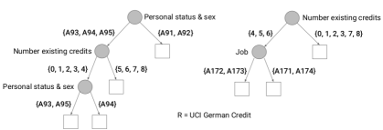
Tables 3 and 4 provide 2D heatmaps of joint densities learned on couples of variables for which the ground truth displays a clear stochastic (sigmacabs) or deterministic (kc1) dependence. At a high level, we see that both generative forests and ensembles of generative trees manage to find very good approximations of the ground truth, with generative forests performing the best among the two kinds of models. Deterministic relationship between observation variables can be explicit from encoding: in the case of compas, features include a one-hot encoding of the age feature. In general, a generative model would not prevent against inconsistencies: in the case of compas, this could result in generating observations with several one-hot encoded features to true. In generative forests, such inconsistencies can naturally be reduced: computing the branching probability at any node (Step 1 in StarUpdate) depends on the training data in the current support . If it involves a one-hot encoded variable, the probability to choose any outcome will be consistent with the previous choices on the other one-hot encoded variables to build . If for example one such previous choice assigns true, the branching probability is guaranteed to be 1 for false at the current one-hot encoded variable (unless, of course, the training data itself contains inconsistencies). In the case of ensembles of generative trees, the property is kept if all occurrences happen in the same tree. The compas example also demonstrates that it is easy to look for dependencies involving sensitive features that could raise fairness issues in the data generation process (unlike deep nets): we have sketched one of the tree in the generative forest. Dashed arcs involve more features (not shown). In this case, we see that the generative model involves sampling the twoyearrecid(ivism) variable within the population of African-Americans having zero juvenile felony counts. Checking the numbers at the leaves of node labeled twoyearrecid, generation tips in favor of twoyearrecid = true (by approximately 57). The second tree can modulate this probability but one can remark that there is no such dependency among variables appearing for non-African-Americans in the generative forest. Note that it would be a simple matter to prevent the induction in gf.Boost to lead to such explicit dependencies by restricting the choices of features to split in splitPred.
| UCI abalone | OpenML analcatdatasupreme | |||
| perr (cat. variables) | rmse (num. variables) | perr | rmse | |
|
vs gf, iterations |
![[Uncaptioned image]](/html/2308.03648/assets/x35.png)
|
![[Uncaptioned image]](/html/2308.03648/assets/x36.png)
|
![[Uncaptioned image]](/html/2308.03648/assets/x37.png)
|
![[Uncaptioned image]](/html/2308.03648/assets/x38.png)
|
|
vs eogtp, iter. |
![[Uncaptioned image]](/html/2308.03648/assets/x39.png)
|
![[Uncaptioned image]](/html/2308.03648/assets/x40.png)
|
![[Uncaptioned image]](/html/2308.03648/assets/x41.png)
|
![[Uncaptioned image]](/html/2308.03648/assets/x42.png)
|
7.2 impute
We compared our method against a powerful contender, mice [37], which relies on round-robin prediction of missing values using supervised models. After an initial prediction of missing values to a default value, mice iteratively predict new values for the missing features of one column given the others imputed and iteratively circles several (=5 by default) times through the columns, repeating the same process. The choice of the method to learn the base predictors is thus important to get the best results and we used tree-based method cart, rf (random forests). To tune mice for better results, we increased the number of trees in a rf from 10 (default) to 100. Our setting parallels that of [23]: we generate missing data (missing completely at random, MCAR) and then impute the missing values from the generative model learned. We replace the optimal transport metric they use by a much finer one which computes a per-feature discrepancy, the average error probability (perr, for categorical variables), and the root mean square error (rmse, for numerical variables). For each mixed feature type domain, we thus have two metrics (otherwise, just the relevant one is computed). We also compute one of the simplest baselines, which consists in imputing each variable from its empirical marginal, shown as marginal.
How to use our models for missing data imputation
Consider generative forests: our generative models allow us to compute the complete joint density of the missing values given the observed ones and a generative model. Being able to impute values is thus a byproduct of this convenience, not the purpose of the method like for mice. A generative forest partitions the domain according to tuples of leaves among its trees. Given a partial assignment of observed variables, it is a simple matter to compute the complete set of tuples that covers the sub-domain of the unknown features: initializing the set of tuples to a singleton being the domain of the missing variables, we descend through each tree (in no order) and eventually update or split the currently available tuples according to the splits in the tree. We then compute the empirical density of all final tuples, proportional to the empirical measure of a tuple over the volume of the domain it defines. Finally, we randomly select a tuple with maximal density and simultaneously sample all missing features uniformly in the tuple’s domain. In a generative forest, this empirical measure can be computed exactly. In an ensemble of generative trees however, this cannot be computed exactly so we rely on the approximation (8) in Lemma 6.2 to compute these.
Results
Table 6 puts the spotlight on two domains. The Appendix summarizes many more plots. From all results, we conclude that generative forests (top row in Table 6) can compete or beat mice.rf while using hundred times less trees (eventually using just stumps, when ). The bottom row, for ensembles of generative trees, displays a predictably more nuanced pattern. Nevertheless, increasing the number of generative trees can still lead to very substantial improvements over a single tree, but necessitates a larger number of iterations () in general ( in Table 6). From all our results, we also conclude that there is a risk of overfitting if and / or are too large and that risk is more prevalent with eogt. This could motivate further work on pruning generative models. For generative forests (gf), an unexpected pattern is that the pattern ”small number of small trees works well” can work on real-world domains as well (see also Appendix), thereby demonstrating that the nice result displayed in Table 1 generalises to bigger domains.
7.3 lifelike
The objective of the experiment is to evaluate whether a generative model is able to create ”realistic” data. Tabular data is hard to evaluate visually, unlike e,g. images or text, so we have considered a simple evaluation pipeline: we create for each domain a 5-fold stratified experiment. After a generative model has been trained, we generate the same number of observations as in the test fold and compute the optimal transport (OT) distance between the generated sample and the fold’s test sample. To fasten the computation of OT costs, we use Sinkhorn’s algorithm [7] with an -entropic regulariser, for some which we observed was the smallest in our experiments to run with all domains without leading to numerical instabilities. To balance the importance of categorical features (for which the cost is binary, depending on whether the guess is right or not) and numerical features, we normalize numerical features with the domain’s mean and standard deviation prior to computing OT costs. We then compare our method to one of two possible contenders: Adversarial Random Forests (ARF) [38] and CT-GAN [41]. Adversarial Random Forests (ARF) are tree-based generators that work as follows to generate one observation: one first sample uniformly at random a tree, then samples a leaf in the tree. The leaf is attached to a distribution which is then used to sample the observation. As we already pointed out in Section 2, there are two main differences with our models. From the standpoint of the model’s distribution, if one takes the (non-empty) support from a tuple of leaves, its probability is obtained from a weighted average of the tree’s distributions in [38] while it is obtained from a product of theirs in our case. Hence, at similar tree sizes, the modelling capability of the set of trees tips in our favor, but it is counterbalanced by the fact that their approach equip leaves with potentially complex distributions (e.g. truncated Gaussians) whereas we stick to uniform distributions at the leaves. A consequence of the modeling of ARFs is that each tree has to separately code for a good generator: hence, it has to be big enough or the distributions used at the leaves have to be complex enough. In our case, as we already pointed out, a small number of trees (sometimes even stumps) can be enough to get a fairly good generator, even on real-world domains. Our second contender, CT-GAN [41], relies on neural networks so it is de facto substantially different from ours.
ARFs are trained with a number of trees . ARFs include an algorithm to select the tree size so we do not have to select it. CT-GANs are trained with a number of epochs . We compare those models with generative forests with trees and trained for a total of iterations, for all domains considered. Compared to the trees learned by ARFs, the total number of splits we use can still be small compared to theirs, in particular when they learn trees. We report results on 13 of our benchmark datasets (not all of them: ARFs cannot be trained on datasets with missing values and we also got some bugs in running the software, see Appendix, Section III.2).
| domain | us (gf) | Adversarial Random Forests (ARFs) | ||||||||
| tag | =500, =2 000 | -val | -val | -val | -val | |||||
| ring | 0.2850.008 | 0.2890.006 | 0.1918 | 0.2860.007 | 0.8542 | 0.2880.010 | 0.7205 | 0.2860.007 | 0.6213 | |
| circ | 0.3510.005 | 0.3540.002 | 0.2942 | 0.3560.008 | 0.2063 | 0.3500.002 | 0.9050 | 0.3550.005 | 0.3304 | |
| grid | 0.3900.002 | 0.3940.003 | 0.1376 | 0.3910.002 | 0.3210 | 0.3920.001 | 0.2118 | 0.3940.002 | 0.0252 | |
| for | 1.1080.105 | 1.2720.281 | 0.2807 | 1.4310.337 | 0.1215 | 1.3110.255 | 0.0972 | 1.2680.209 | 0.0616 | |
| rand | 0.2860.003 | 0.2860.003 | 0.9468 | 0.2900.005 | 0.2359 | 0.2890.005 | 0.3990 | 0.2880.002 | 0.3685 | |
| tic | 0.5750.002 | 0.5770.001 | 0.2133 | 0.5780.001 | 0.1104 | 0.5770.001 | 0.2739 | 0.5770.001 | 0.2773 | |
| iono | 1.1670.074 | 1.4310.043 | 0.0005 | 1.4690.079 | 0.0001 | 1.4310.058 | 0.0015 | 1.4200.056 | 0.0035 | |
| stm | 0.9750.026 | 1.0100.015 | 0.0304 | 1.0150.018 | 0.0231 | 1.0010.010 | 0.0956 | 1.0140.021 | 0.0261 | |
| wred | 0.9800.032 | 1.0860.036 | 0.0003 | 1.0720.055 | 0.0133 | 1.0860.030 | 0.0003 | 1.0990.031 | 0.0001 | |
| stp | 0.9760.018 | 0.9990.011 | 0.0382 | 1.0120.010 | 0.0250 | 1.0060.011 | 0.0280 | 1.0030.003 | 0.0277 | |
| ana | 0.3680.014 | 0.3700.012 | 0.7951 | 0.3820.015 | 0.1822 | 0.3680.006 | 0.9161 | 0.3690.007 | 0.8316 | |
| aba | 0.4900.028 | 0.5050.046 | 0.5251 | 0.4840.024 | 0.7011 | 0.5030.035 | 0.6757 | 0.4810.031 | 0.4632 | |
| wwhi | 1.0640.003 | 1.1590.011 | 1.1590.006 | 1.1700.014 | 1.1500.021 | 0.0005 | ||||
| wins / lose for us | 12 / 0 | 12 / 1 | 11 / 1 | 12 / 1 | ||||||
Results vs ARFs
Table 7 presents the results obtained against adversarial random forests. A first observation, not visible in the table, is that ARFs indeed tend to learn big models, typically with dozens of nodes in each tree. For the largest ARFs with 100 or 200 trees, this means in general a total of thousands of nodes in models. A consequence, also observed experimentally, is that there is little difference in performance in general between models with a different number of trees in ARFs as each tree is in fact an already good generator. In our case, this is obviously not the case. Noticeably, the performance of ARFs is not monotonic in the number of trees, so there could be a way to find the appropriate number of trees in ARFs to buy the slight (but sometimes significant) increase in performance in a domain-dependent way. In our case, there is obviously a dependency in the number of trees chosen as well. From the standpoint of the optimal transport metric, even when ARFs make use of distributions at their tree leaves that are much more powerful than ours and in fact fit to some of our simulated domains (Gaussians used in circgauss, randgauss and gridgauss), we still manage to compete or beat ARFs on those simulated domains.
Globally, we manage to beat ARFs on almost all runs, and very significantly on many of them. Since training generative forests does not include a mechanism to select the size of models, we have completed this experiment by another one on which we learn much smaller generative forests. The corresponding Table is in Appendix, Section III.III.3.4. Because we cleatly beat ARFs on studentperformancemat and studentperformancepor in Table 7 but are beaten by ARFs for much smaller generative forests, we conclude that there could exist mechanisms to compute the ”right size” of our models. Globally however, even with such smaller models, we still manage to beat ARFs on a large majority of cases, which is a good figure given the difference in model sizes. The ratio ”results quality over model size” tips in our favor and demonstrates the potential in using all trees in a forest to generate an observation (us) vs using a single of its trees (ARFs), see Figure 1.
Results vs CT-GANs
Table 8 summarizes our results against CT-GAN using various numbers of training epochs. In our case, our setting is the same as versus ARFs: we stick to trees trained for a total number of iterations in the generative forest, for all domains. We see that generative forests consistently and significantly outperform CT-GAN on nearly all cases. Furthermore, while CT-GANs performances tend to improve with the number of epochs, we observe that on a majority of datasets, performances at 1 000 epochs are still far from those of generative forests and already induce training times that are far bigger than for generative forests: for example, more than 6 hours per fold for stm while it takes just a few seconds to train a generative forest. Just like we did for ARFs, we repeated the experiment vs CT-GAN using much smaller generative forests (). The results are presented in Appendix, Section III.III.3.4. There is no change in the conclusion: even with such small models, we still beat CT-GANs, regardless of the number of training epochs, on all cases (and very significantly on almost all of them).
| domain | us (gf) | CT-GANs | ||||||||
| tag | =500, =2 000 | -val | -val | -val | -val | |||||
| ring | 0.2850.008 | 0.4570.058 | 0.0032 | 0.5460.079 | 0.0018 | 0.4050.044 | 0.0049 | 0.3510.042 | 0.0183 | |
| circ | 0.3510.005 | 0.8480.300 | 0.0213 | 0.4800.040 | 0.0019 | 0.4430.014 | 0.4350.075 | 0.0711 | ||
| grid | 0.3900.002 | 0.7490.417 | 0.1268 | 0.4590.031 | 0.0085 | 0.4260.022 | 0.0271 | 0.4080.019 | 0.1000 | |
| for | 1.1080.105 | 9.7965.454 | 0.0049 | 1.8990.289 | 0.0045 | 1.5320.178 | 0.0244 | 1.5200.311 | 0.0410 | |
| rand | 0.2860.003 | 0.7460.236 | 0.0119 | 0.4910.063 | 0.0021 | 0.3680.015 | 0.0002 | 0.3270.024 | 0.0288 | |
| tic | 0.5750.002 | 0.6010.003 | 0.0002 | 0.5810.001 | 0.0082 | 0.5860.006 | 0.0294 | 0.5840.003 | 0.0198 | |
| iono | 1.1670.074 | 2.2630.035 | 2.0840.052 | 1.9840.136 | 1.7580.137 | 0.0002 | ||||
| stm | 0.9800.032 | 1.5110.074 | 1.1890.045 | 0.0002 | 1.1680.054 | 0.0056 | 1.1670.041 | 0.0013 | ||
| wred | 0.9800.032 | 2.8360.703 | 0.0044 | 2.0040.090 | 1.8250.127 | 0.0001 | 1.3840.047 | |||
| stp | 0.9760.018 | 1.6600.161 | 0.0006 | 1.1410.018 | 0.0001 | 1.2060.046 | 0.0007 | 1.1860.052 | 0.0019 | |
| ana | 0.3680.014 | 0.5420.135 | 0.0050 | 0.4390.056 | 0.0202 | 0.4040.012 | 0.0397 | 0.4360.036 | 0.0051 | |
| aba | 0.4900.028 | 1.6890.053 | 1.4630.094 | 0.7540.040 | 0.0009 | 0.6570.026 | 0.0006 | |||
| wwhi | 1.0640.003 | 1.7700.160 | 0.0005 | 1.8490.064 | 1.2840.029 | 1.1580.009 | ||||
| wins / lose for us | 13 / 0 | 13 / 0 | 13 / 0 | 13 / 0 | ||||||
Preliminary results vs an ”optimal generator”
are presented in Appendix (Subsection III.III.3.5), in which we design a pipeline allowing to compare generated data against real data, displaying that on some small domains at least, we can manage to generate data that looks as real as the domain itself.
8 Conclusion
In this paper, we propose new models and training algorithms for generative models that generalize the recently introduced generative trees [23]. Our models, generative forests, leverage the combinatorics that sets of trees can have compared to trees to partition a tabular domain. We show how to train generative forests in a supervised learning framework, simplifying the GAN approach for generative trees of [23], while keeping boosting-compliant convergence in a generative metric, also extending the scope of convergence compared to [23]. Experiments display the potential of small generators (even containing tree stumps) and suggest an interesting research direction on pruning algorithms for tree-based generative models.
A big difference with [23] and other generative approaches is from the standpoint of code reusability: gf.Boost can be implemented using standard codes for training decision trees with two classes, in just a few tweaks to adapt the model and replace negative examples by straightforward length computations. Considering the vast amount of existing code in general repositories (thousands in GitHub) to its use in popular ML tools [26, 3, 39], this could represent a good basis for the implementation and adoption of gf.Boost. From this standpoint, training ensembles of generative trees instead of generative forests could represent an even simpler implementation choice.
References
- [1] L. Breiman, J. H. Freidman, R. A. Olshen, and C. J. Stone. Classification and regression trees. Wadsworth, 1984.
- [2] A. Buja, W. Stuetzle, and Y. Shen. Loss functions for binary class probability estimation ans classification: structure and applications, 2005. Technical Report, University of Pennsylvania.
- [3] T. Chen and C. Guestrin. XGBoost: A scalable tree boosting system. In 22nd KDD, pages 785–794, 2016.
- [4] Y. Choi, A. Vergari, and G. Van den Broeck. Probabilistic circuits: a unifying framework for tractable probabilistic models, 2020. http://starai.cs.ucla.edu/papers/ProbCirc20.pdf.
- [5] M. Chui, J. Manyika, M. Miremadi, N. Henke, R. Chung P. Nel, and S. Malhotra. Notes from the AI frontier. McKinsey Global Institute, 2018.
- [6] A.-H.-C. Correia, R. Peharz, and C.-P. de Campos. Joints in random forests. In NeurIPS’20, 2020.
- [7] M. Cuturi. Sinkhorn distances: lightspeed computation of optimal transport. In NIPS*26, pages 2292–2300, 2013.
- [8] D. Dua and C. Graff. UCI machine learning repository, 2021.
- [9] V. Dumoulin, I. Belghazi, B. Poole, A. Lamb, M. Arjovsky, O. Mastropietro, and A.-C. Courville. Adversarially learned inference. In ICLR’17. OpenReview.net, 2017.
- [10] I. Goodfellow, J. Pouget-Abadie, M. Mirza, B. Xu, D. Warde-Farley, S. Ozair, A. Courville, and Y. Bengio. Generative adversarial nets. In NIPS*27, pages 2672–2680, 2014.
- [11] A. Grover and S. Ermon. Boosted generative models. In AAAI’18, pages 3077–3084. AAAI Press, 2018.
- [12] G.-E. Hinton. The forward-forward algorithm: Some preliminary investigations. CoRR, abs/2212.13345, 2022.
- [13] M. Hulsebos, H. Dong, B. Karlas, L. Orr, and P. Yin. Table Representation Learning Workshop. NeurIPS’22, 2022.
- [14] M.J. Kearns. Thoughts on hypothesis boosting, 1988. ML class project.
- [15] M.J. Kearns and Y. Mansour. On the boosting ability of top-down decision tree learning algorithms. In Proc. of the 28 ACM STOC, pages 459–468, 1996.
- [16] D.-P. Kingma and M. Welling. Auto-encoding variational bayes. In ICLR’14, 2014.
- [17] D.-E. Knuth. Two notes on notation. The American Mathematical Monthly, 99(5):403–422, 1992.
- [18] Y. Mansour, R. Nock, and R.-C. Williamson. What killed the convex booster ? CoRR, abs/2205.09628, 2022.
- [19] Y. Mansour, R. Nock, and R.-C. Williamson. Random classification noise does not defeat all convex potential boosters irrespective of model choice. In ICML’23, 2023.
- [20] P. Maréchal. On a functional operation generating convex functions, part 1: duality. J. of Optimization Theory and Applications, 126:175–189, 2005.
- [21] P. Maréchal. On a functional operation generating convex functions, part 2: algebraic properties. J. of Optimization Theory and Applications, 126:375–366, 2005.
- [22] A. Menon and C.-S. Ong. Linking losses for density ratio and class-probability estimation. In 33rd ICML, pages 304–313, 2016.
- [23] R. Nock and M. Guillame-Bert. Generative trees: Adversarial and copycat. In 39th ICML, pages 16906–16951, 2022.
- [24] R. Nock, A.-K. Menon, and C.-S. Ong. A scaled Bregman theorem with applications. In NIPS*29, pages 19–27, 2016.
- [25] R. Nock and F. Nielsen. On the efficient minimization of classification-calibrated surrogates. In NIPS*21, pages 1201–1208, 2008.
- [26] F. Pedregosa, G. Varoquaux, A. Gramfort, V. Michel, B. Thirion, O. Grisel, M. Blondel, P. Prettenhofer, R. Weiss, V. Dubourg, J. Vanderplas, A. Passos, D. Cournapeau, M. Brucher, M. Perrot, and E. Duchesnay. Scikit-learn: Machine learning in Python. Journal of Machine Learning Research, 12:2825–2830, 2011.
- [27] H. Poon and P.-M. Domingos. Sum-product networks: A new deep architecture. In UAI’11, pages 337–346. AUAI Press, 2011.
- [28] J. R. Quinlan. C4.5 : programs for machine learning. Morgan Kaufmann, 1993.
- [29] T. Rahman, P.-V. Kothalkar, and V. Gogate. Cutset networks: A simple, tractable, and scalable approach for improving the accuracy of Chow-Liu trees. In ECMLPKDD’14, volume 8725 of Lecture Notes in Computer Science, pages 630–645. Springer, 2014.
- [30] M.-D. Reid and R.-C. Williamson. Information, divergence and risk for binary experiments. JMLR, 12:731–817, 2011.
- [31] C. Roy, T. Rahman, H. Dong, N. Ruozzi, and V. Gogate. Dynamic cutset networks. In AISTATS’21, volume 130 of Proceedings of Machine Learning Research, pages 3106–3114. PMLR, 2021.
- [32] R. Sánchez-Cauce, I. París, and F.-J. Díez. Sum-product networks: A survey. IEEE Trans.PAMI, 44(7):3821–3839, 2022.
- [33] L.-J. Savage. Elicitation of personal probabilities and expectations. J. of the Am. Stat. Assoc., pages 783–801, 1971.
- [34] R. E. Schapire and Y. Singer. Improved boosting algorithms using confidence-rated predictions. In 9 COLT, pages 80–91, 1998.
- [35] A. Soen, H. Husain, and R. Nock. Fair densities via boosting the sufficient statistics of exponential families. In ICML’23, 2023.
- [36] M. Sugiyama and M. Kawanabe. Machine Learning in Non-Stationary Environments - Introduction to Covariate Shift Adaptation. Adaptive computation and machine learning. MIT Press, 2012.
- [37] S. van Buuren and K. Groothuis-Oudshoorn. mice: Multivariate Imputation by Chained Equations in R. Journal of Statistical Software, 45(3):1–67, 2011.
- [38] D.-S. Watson, K. Blesch, J. Kapar, and M.-N. Wright. Adversarial random forests for density and generative modeling. In AISTATS’23, Proceedings of Machine Learning Research. PMLR, 2023.
- [39] I. Witten and E. Frank. Data Mining: Practical Machine Learning Tools and Techniques with Java Implementations. Morgan Kaufmann, 1999.
- [40] C. Xiao, P. Zhong, and C. Zheng. BourGAN: Generative networks with metric embeddings. In NeurIPS’18, pages 2275–2286, 2018.
- [41] L. Xu, M. Skoularidou, A. Cuesta-Infante, and K. Veeramachaneni. Modeling tabular data using conditional GAN. In NeurIPS*32, pages 7333–7343, 2019.
Appendix
To differentiate with the numberings in the main file, the numbering of Theorems, etc. is letter-based (A, B, …).
Table of contents
Additional content Pg I
Supplementary material on proofs Pg
II
Proof of Lemma 4.4 Pg II.1
Proof of Theorem 5.2 Pg II.2
Proof of Lemma 6.2 Pg II.3
Supplementary material on experiments Pg
III
Domains Pg III.1
Algorithms configuration and choice of parameters Pg III.2
More examples of Table 1 (mf) Pg III.III.3.1
The generative forest of Table 1 (mf) developed further Pg III.III.3.2
Full comparisons with mice on missing data imputation Pg III.III.3.3
Remaining tables for experiment lifelike Pg III.III.3.4
Comparison with ”the optimal generator”: gen-discrim Pg III.III.3.5
Appendix I Additional content
In this additional content, we focus on providing other examples to IterativeSupportUpdate (Algorithm 3) and a proof that the optimal splitting threshold on a continuous variable when training a generative forest using gf.Boost is always an observed value if there is one tree, but can be another value if there are more.
I.1 Concurrent generation of observations
We provide a concurrent generation using Algorithm 5, which differs from Algorithm 3 (main file). In concurrent generation, each tree runs concurrently algorithm UpdateSupport (hence the use of the Java-style this handler), with an additional global variables (in addition to , initialized to ): a Boolean semaphore accessible implementing a lock, whose value 1 means is available for an update (and otherwise it is locked by a tree in Steps 1.2/1.3 in the set of trees of the gf). We assume that Init has been run beforehand (eventually locally).
I.2 Randomized generation of observations
We provide a general randomized choice of the sequence of trees for generation, in Algorithm 6.
I.3 Optimal thresholds for continuous variables
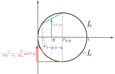
Our generative models use predicates based on axis-parallel splits. For features designed on countable sets, finding the optimal split that minimizes (5) – which trivially depends on observed values – is simple if the number of observed values is not too large. For continous values however, the question arises as to what do the optimal splits minimizing (5) look like. Our assumptions on the loss used being very loose, we can show that finding the optimal split is not as trivial in the most general case, but there is one notable exception: if the forest contains a single tree, the optimal split also occur at an observed value.
Lemma A.
Suppose contains one tree and the variable chosen at Step 2.3 of gf.Boost is continuous, with observed distinct modalities for some . Within any interval of possible values () for the threshold, the optimal threshold minimizing (5) is either at or . This is no longer true if contains two trees or more.
Proof:
Note: we shall make the assumption that is finite, without loss of generality. Denote the subset of whose elements are defined by an intersection with the support of , . Minimizing Bayes risk amounts to minimizing the contribution of a new split at the candidate leaf ,
where
| (10) |
with . Suppose the feature chosen for the split is continuous and we have a current threshold guess at the implementation of the corresponding splitting predicate p. We assume that the range of possible values for includes interval where are two observed values with no more observed values in and the current
is in .
We first show that if is a singleton, the optimal is always at an observed value. Denote , which is a constant . Let
| (11) |
and we have for some constant , because is an affine function of , but . Assuming differentiable, we thus get
with . Assuming finite, we can also note , so that we simplify
Denote for short , so that we can write:
| (12) |
Assuming strictly concave, is strictly increasing in and so zeroes iff
which corresponds to a maximum of , not a minimum. Otherwise, takes on one sign only. Figure 5 provides a graphical viewpoint of all key parameters. We observe
| (13) |
Hence, to decrease , we need to increase iff , hence iff . Otherwise, if (or ), we need to decrease . We thus get two possible locally optimal predicates compared to the current choice (and whether the current inequality is strict or not):
-
1.
, when we currently have . This reduces further and decreases ;
-
2.
, when we currently have . This increases further and decreases .
Notice that in the second case, we can make the inequality large and further decrease , because it decreases without changing . There is a simple check if satisfies : we can rewrite, for an equivalent change in that would affect only but not ,
Wanting (we decrease by changing the inequality to large at ) imposes , i.e. , allowing us to replace the splitting predicate by in [2.] above.
Using the same technique, we can show that as soon as contains two elements (which can be the case with any number of trees greater than 1), the optimal threshold may not be at an observed value anymore. To see this, we just compute the first order condition for to zero within where are two observed values with no more observed value in between. We get from (12), using two and instead of one, the condition that
| (14) |
with
| (15) |
The positivity condition (assuming wlog the denominator is not zero) imposes a different ordering between the and , which from (13) imposes and or and . Apart from this condition, the two elements in relate to two different leaves whose support do not intersect and such that the derivative is a constant proportional to the measure alongside variable of their support. If (resp. ) belongs to the range of values that (resp. ) takes when sliding in , then by sliding in the RHS in (14) covers and since it is a continuous function, must take value for some . To design a minimum at some , we factor the derivative, considering , i.e. we simplify to :
with
For , we know that . To get a minimum at , it is necessary that if we decrease below and if we increase above . Hence, it is sufficient that increases as a function of while decreases as a function of . From the previous case, it is then sufficient that at we have .
Appendix II Supplementary material on proofs
II.1 Proof of Lemma 4.4
Given sequence of dimension , denote the sequence of subsets of the domain appearing in the parameters of UpdateSupport through sequence , to which we add a last element, (and its first element is ). If we let denote the support of the corresponding star node whose Bernoulli event is triggered at index in sequence (for example, ), then we easily get
| (16) |
indicating the Bernoulli probability in Step 1.1 of StarUpdate is always defined. We then compute
| (17) | |||||
| (18) | |||||
| (19) | |||||
| (21) |
(18) holds because updating the support generation is Markovian in a gf, (19) holds because of Step 3.2 and (II.1) is a simplification through cancelling terms in products.
II.2 Proof of Theorem 5.2
Notations: we iteratively learn generators where is just a root. We let denote the partition induced by the set of trees of , recalling that each element is the (non-empty) intersection of the support of a set of leaves, one for each tree (for example, ). The criterion minimized to build from is
| (22) |
The proof entails fundamental notions on loss functions, models and boosting. We start with loss functions. A key function we use is
which is concave [30, Appendix A.3].
Lemma A.
| (23) |
Proof.
We make us of the following important fact about gfs:
-
(F1)
For any , .
We have from the proof of [23, Lemma 5.6],
| (24) |
We note that (F1) implies (24) is just a sum of slacks of Jensen’s inequality. We observe
where contains all couples such that and . These unions were subsets of the partition of induced by the set of trees of and that were cut by the predicate p put at the leaf that created from . To save space, denote .
| (25) | |||||
We now work on (25). Using (F1), we note since . Similarly, , so we make appear in (25) and get:
| (26) | |||||
where we let for short
| (27) |
We finally get
as claimed. The last identity comes from the fact that the contribution to is the same outside for both and . ∎
We now come to models and boosting. Suppose we have trees in . We want to split leaf into two new leaves, . Let denote the subset of containing only the subsets defined by intersection with the support of , . The criterion we minimize can be reformulated as
Here, is any tree in the set of trees, since covers the complete partition of induced by . If we had a single tree, the inner sum would disappear since we would have and so one iteration would split one of these subsets. In our case however, with a set of trees, we still split but the impact on the reduction of can be substantially better as we may simultaneously split as many subsets as there are in . The reduction in can be obtained by summing all reductions to which contribute each of the subsets.
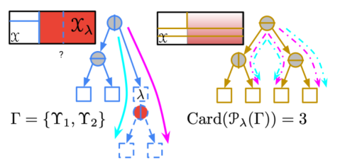
To analyze it, we make use of a reduction to the ModaBoost algorithm of [18]. We present the algorithm in Algorithm 7.
| (28) | |||||
| (29) | |||||
| (30) | |||||
| (31) |
| (32) |
The original ModaBoost algorithm trains partition-linear models, i.e. models whose output is defined by a sum of reals over a set of partitions to which the observation to be classified belongs to. Training means then both learning the organisation of partitions and the reals – which are just the output of a weak classifier given by a weak learner, times a leveraging constant computed by ModaBoost. As in the classical boosting literature, the original ModaBoost includes the computation and updates of weights.
In our case, the structure of partition learned is that of a set of trees, each weak classifier is of the form
where is a real and p is a Boolean predicate, usually doing an axis-parallel split of on an observed feature, such as .
From now on, it will be interesting to dissociate our generator – which includes a model structure and an algorithm to generate data from this structure– from its set of trees – i.e. its model structure – which we denote . ModaBoost learns both but also predictions for each possible outcome, predictions that we shall not use since the loss we are minimizing can be made to depend only on the model structure . Given the simplicity of the weak classifiers and the particular nature of the partitions learned, the original ModaBoost of [18] can be simplified to our presentation in Algorithm 7. Among others, the simplification discards the weights from the presentation of the algorithm. What we show entangles two objectives on models and loss functions as we show that
ModaBoost learns the same structure as our gf.Boost, and yields a guaranteed decrease of ,
and it is achieved via the following Theorem.
Theorem B.
ModaBoost greedily minimizes the following loss function:
Furthermore, suppose there exists such that at each iteration , the predicate p splits of leaf into and (same nomenclature as in (28), (30)) such that:
| (33) | |||||
| (34) | |||||
| (35) |
Then we have the following guaranteed slack between two successive models:
| (36) |
where is such that .
Proof sketch The loss function comes directly from [18, Lemma 7]. At each iteration, ModaBoost makes a number of updates that guarantee, once Step 2.4 is completed (because the elements in are disjoint)
| (37) | |||||
| (38) |
where the weights are given in [18]. Each expression in the summand of (37) is exactly the guarantee of [18, ineq. before (69)]; all such expressions are not important; what is more important is (37): all steps occurring in Step 2.4 are equivalent to a single step of ModaBoost carried out over the whole . Overall, the number of ”aggregated” steps match the counter in ModaBoost. We then just have to reuse the proof of [18, Theorem B], which implies, in lieu of their [18, eq. (74)]
| (39) |
with . Noting , we then use (33) – (35), which yields the statement of the Theorem.
As a consequence, if we assume that the total number of boosting iterations is a multiple of the number of trees , it comes from [18, eq. (29)] that after iterations, we have
| (40) |
Using Lemma A and the fact that the induction of the sets of trees in ModaBoost is done in the same way as the induction of the set of trees of our generator in gf.Boost, we get:
as claimed.
II.3 Proof of Lemma 6.2
Because at any call of StarUpdate, we have
| (41) | |||||
| (43) | |||||
(43) is due to the fact that, since , , and then using (7). (43) is obtained by dividing numerator and denominator by .
and satisfy so
| (44) | |||||
| (45) |
Finally, and are just the product of the branching probabilities in any admissible sequence. If we use the same admissible sequence in both generators, we can write and , and (43) directly yields , being a shorthand for (see main file). So, for any ,
| (46) |
and finally, replacing back by notation ,
| (47) | |||||
as claimed.
Appendix III Appendix on experiments
III.1 Domains
| Domain | Tag | Source | Missing data | Cat. | Num. | ||
| iris | – | UCI | No | 150 | 5 | 1 | 4 |
| ∗ringGauss | ring | – | No | 1 600 | 2 | – | 2 |
| ∗circGauss | circ | – | No | 2 200 | 2 | – | 2 |
| ∗gridGauss | grid | – | No | 2 500 | 2 | – | 2 |
| forestfires | for | OpenML | No | 517 | 13 | 2 | 11 |
| ∗randGauss | rand | – | No | 3 800 | 2 | – | 2 |
| tictactoe | tic | UCI | No | 958 | 9 | 9 | – |
| ionosphere | iono | UCI | No | 351 | 34 | 2 | 32 |
| studentperformancemat | stm | UCI | No | 396 | 33 | 17 | 16 |
| winered | wred | UCI | No | 1 599 | 12 | 12 | – |
| studentperformancepor | stp | UCI | No | 650 | 33 | 17 | 16 |
| analcatdatasupreme | ana | OpenML | No | 4 053 | 8 | 1 | 7 |
| abalone | aba | UCI | No | 4 177 | 9 | 1 | 8 |
| kc1 | – | OpenML | No | 2 110 | 22 | 1 | 21 |
| winewhite | wwhi | UCI | No | 4 898 | 12 | 12 | – |
| sigma-cabs | – | Kaggle | Yes | 5 000 | 13 | 5 | 8 |
| compas | – | OpenML | No | 5 278 | 14 | 9 | 5 |
| open-policing-hartford | – | SOP | Yes | 18 419 | 20 | 16 | 4 |
ringGauss is the seminal 2D ring Gaussians appearing in numerous GAN papers [40]; those are eight (8) spherical Gaussians with equal covariance, sampling size and centers located on regularly spaced (2-2 angular distance) and at equal distance from the origin. gridGauss was generated as a decently hard task from [9]: it consists of 25 2D mixture spherical Gaussians with equal variance and sampled sizes, put on a regular grid. circGauss is a Gaussian mode surrounded by a circle, from [40]. randGauss is a substantially harder version of ringGauss with 16 mixture components, in which covariance, sampling sizes and distances on sightlines from the origin are all random, which creates very substantial discrepancies between modes.
III.2 Algorithms configuration and choice of parameters
gf.Boost
We have implemented gf.Boost in Java, following Algorithm 4’s blueprint. Our implementation of tree and leaf in Steps 2.1, 2.2 is simple: we pick the heaviest leaf among all trees (with respect to ). The search for the best split is exhaustive unless the variable is categorical with more than a fixed number of distinct modalities (22 in our experiments), above that threshold, we pick the best split among a random subset. We follow [23]’s experimental setting: in particular, the input of our algorithm to train a generator is a .csv file containing the training data without any further information. Each feature’s domain is learned from the training data only; while this could surely and trivially be replaced by a user-informed domain for improved results (e.g. indicating a proportion’s domain as , informing the complete list of socio-professional categories, etc.) — and is in fact standard in some ML packages like weka’s ARFF files, we did not pick this option to alleviate all side information available to the GT learner. Our software automatically recognizes three types of variables: nominal, integer and floating point represented.
mice
We have used the R mice package V 3.13.0 with two choices of methods for the round robin (column-wise) prediction of missing values: cart [1] and random forests (rf) [37]. In that last case, we have replaced the default number of trees (10) by a larger number (100) to get better results. We use the default number of round-robin iterations (5). We observed that random forests got the best results so, in order not to multiply the experiments reported and perhaps blur the comparisons with our method, we report only mice’s results for random forests.
TensorFlow
To learn the additional Random Forests involved in experiments gen-discrim, we used Tensorflow Decision Forests library†††https://github.com/google/yggdrasil-decision-forests/blob/main/documentation/learners.md. We use 300 trees with max depth 16. Attribute sampling: sqrt(number attributes) for classification problems, number attributes / 3 for regression problems (Breiman rule of thumb); the min examples per leaf is 5.
Adversarial Random Forests
We used the R code of the generator forge made available from the paper [38]‡‡‡https://github.com/bips-hb/arf_paper, learning forests containing a variable number of trees in . We noted that the code does not run when the dataset has missing values and we also got an error when trying to run the code on kc1.
Computers used
We ran part of the experiments on a Mac Book Pro 16 Gb RAM w/ 2 GHz Quad-Core Intel Core i5 processor, and part on a desktop Intel(R) Xeon(R) 3.70GHz with 12 cores and 64 Gb RAM.
III.3 Supplementary results
Due to the sheer number of tables to follow, we shall group them according to topics
III.III.3.1 More examples of Table 1 (mf)
We provide in Table A10 the density learned on all our four 2D (for easy plotting) simulated domains and not just circgauss as in Table 1 (mf). We see that the observations made in Table 1 (mf) can be generalized to all domains. Even when the results are less different between 50 stumps in a generative forest and 1 generative tree with 50 splits for ringgauss and randgauss, the difference on gridgauss is stark, 1 generative tree merging many of the Gaussians.
![[Uncaptioned image]](/html/2308.03648/assets/x45.png)
III.III.3.2 The generative forest of Table 1 (mf) developed further
One might wonder how a set of stumps gets to accurately fit the domain as the number of stumps increases. Table A11 provides an answer. From this experiment, we can see that 16 stumps are enough to get the center mode. The ring shape takes obviously more iterations to represent but still, is takes a mere few dozen stumps to clearly get an accurate shape, the last iterations just finessing the fitting.
![[Uncaptioned image]](/html/2308.03648/assets/x46.png)
III.III.3.3 Full comparisons with mice on missing data imputation
The main file provides just two examples of domains for the comparison, abalone and analcatdatasupreme. We provide here more complete results on the domain used in the main file and results on more domains in the form of one table for each additional domain:
- •
- •
-
(tables below are ordered in increasing domain size, see Table A9)
-
•
Table A14: experiments on iris;
-
•
Table A15: experiments on ringgauss;
-
•
Table A16: experiments on circgauss;
-
•
Table A17: experiments on gridgauss;
-
•
Table A18: experiments on randgauss;
-
•
Table A19: experiments on studentperformancemat;
-
•
Table A20: experiments on studentperformancepor;
-
•
Table A21: experiments on kc1;
-
•
Table A22: experiments on sigmacabs;
-
•
Table A23: experiments on compas;
-
•
Table A24: experiments on openpolicinghartford;
The large amount of pictures to process may make it difficult to understand at first glance how our approaches behave against mice, so we summarize here the key points:
-
•
first and most importantly, there is not one single type of our models that perform better than the other. Both Generative Forests and Ensembles of Generative Trees can be useful for the task of missing data imputation. For example, analcatdatasupreme gives a clear advantage to Generative Forests: they even beat mice with random forests having 4 000 trees (that is hundreds of times more than our models) on both categorical variables (perr) and numerical variables (rmse). However, on circgauss, studentperformancepor and sigmacabs, Ensembles of Generative Trees obtain the best results. On sigmacabs, they can perform on par with mice if the number of tree is limited (which represents 100+ times less trees than mice’s models);
-
•
as is already noted in the main file (mf) and visible on several plots (see e,g, sigmacabs), overfitting can happen with our models (both Generative Forests and Ensembles of Generative Trees), which supports the idea that a pruning mechanism or a mechanism to stop training would be a strong plus to training such models. Interestingly, in several cases where overfitting seems to happen, increasing the number of splits can reduce the phenomenon, at fixed number of trees: see for example iris ( iterations for eogts), gridgauss, randgauss and kc1 (gfs);
-
•
some domains show that our models seem to be better at estimating continuous (regression) rather than categorical (prediction) variables: see for example abalone, studentperformancemat, studentperformancepor and our biggest domain, openpolicinghartford. Note from that last domain that a larger number of iterations or models with a larger number of trees may be required for the best results, in particular for Ensembles of Generative Trees;
-
•
small models may be enough to get excellent results on real world domains whose size would, at first glance, seem to require much bigger ones: on compas, we can compete (rmse) or beat (perr) mice whose models contain 7 000 trees with just 20 stumps;
-
•
it is important to remember that our technique does not just offer the capability to do missing data imputation: our models can also generate data and compute the full density conditional to observed values, which is not the case of mice’s models, crafted with the sole purpose of solving the task of missing data imputation. Our objective was not to beat mice, but rather show that Generative Forests and Ensembles of Generative Trees can also be useful for this task.
![[Uncaptioned image]](/html/2308.03648/assets/x47.png)
![[Uncaptioned image]](/html/2308.03648/assets/x48.png)
![[Uncaptioned image]](/html/2308.03648/assets/x49.png)
![[Uncaptioned image]](/html/2308.03648/assets/x50.png)
![[Uncaptioned image]](/html/2308.03648/assets/x51.png)
![[Uncaptioned image]](/html/2308.03648/assets/x52.png)
![[Uncaptioned image]](/html/2308.03648/assets/x53.png)
![[Uncaptioned image]](/html/2308.03648/assets/x54.png)
![[Uncaptioned image]](/html/2308.03648/assets/x55.png)
![[Uncaptioned image]](/html/2308.03648/assets/x56.png)
![[Uncaptioned image]](/html/2308.03648/assets/x57.png)
![[Uncaptioned image]](/html/2308.03648/assets/x58.png)
![[Uncaptioned image]](/html/2308.03648/assets/x59.png)
III.III.3.4 Remaining tables for experiment lifelike
| domain | us (gf) | Adversarial Random Forests (ARFs) | ||||||||
| tag | =200, =500 | -val | -val | -val | -val | |||||
| ring | 0.2830.005 | 0.2890.006 | 0.0651 | 0.2860.007 | 0.4903 | 0.2880.010 | 0.4292 | 0.2860.007 | 0.7442 | |
| circ | 0.3560.002 | 0.3540.002 | 0.4561 | 0.3560.008 | 0.7882 | 0.3500.002 | 0.0591 | 0.3550.005 | 0.7446 | |
| grid | 0.3920.002 | 0.3940.003 | 0.4108 | 0.3910.002 | 0.3403 | 0.3920.001 | 0.8370 | 0.3940.002 | 0.3423 | |
| for | 1.0860.124 | 1.2720.281 | 0.1420 | 1.4310.337 | 0.1142 | 1.3110.255 | 0.1215 | 1.2680.209 | 0.0370 | |
| rand | 0.2900.007 | 0.2860.003 | 0.4488 | 0.2900.005 | 0.9553 | 0.2890.005 | 0.9004 | 0.2880.002 | 0.6542 | |
| tic | 0.5740.001 | 0.5770.001 | 0.0394 | 0.5780.001 | 0.0325 | 0.5770.001 | 0.0657 | 0.5770.001 | 0.0914 | |
| iono | 1.4100.116 | 1.4310.043 | 0.7307 | 1.4690.079 | 0.3402 | 1.4310.058 | 0.7046 | 1.4200.056 | 0.8737 | |
| stm | 1.0440.013 | 1.0100.015 | 0.0080 | 1.0150.018 | 0.0094 | 1.0010.010 | 0.0037 | 1.0140.021 | 0.0329 | |
| wred | 1.0270.037 | 1.0860.036 | 0.0327 | 1.0720.055 | 0.1432 | 1.0860.030 | 0.0095 | 1.0990.031 | 0.0044 | |
| stp | 1.0290.027 | 0.9990.011 | 0.0826 | 1.0120.010 | 0.3421 | 1.0060.011 | 0.0542 | 1.0030.003 | 0.0764 | |
| ana | 0.3670.018 | 0.3700.012 | 0.8229 | 0.3820.015 | 0.2318 | 0.3680.006 | 0.9264 | 0.3690.007 | 0.8722 | |
| aba | 0.4760.017 | 0.5050.046 | 0.2264 | 0.4840.024 | 0.2162 | 0.5030.035 | 0.1847 | 0.4810.031 | 0.7468 | |
| wwhi | 1.1200.013 | 1.1590.011 | 0.0013 | 1.1590.006 | 0.0014 | 1.1700.014 | 0.0026 | 1.1500.021 | 0.0327 | |
| wins / lose for us | 9 / 4 | 8 / 3 | 8 / 4 | 9 / 4 | ||||||
| domain | us (gf) | CT-GANs | ||||||||
| tag | =200, =500 | -val | -val | -val | -val | |||||
| ring | 0.2830.005 | 0.4570.058 | 0.0029 | 0.5460.079 | 0.0020 | 0.4050.044 | 0.0048 | 0.3510.042 | 0.0299 | |
| circ | 0.3560.002 | 0.8480.300 | 0.0217 | 0.4800.040 | 0.0024 | 0.4430.014 | 0.0001 | 0.4350.075 | 0.0816 | |
| grid | 0.3920.002 | 0.7490.417 | 0.1279 | 0.4590.031 | 0.0096 | 0.4260.022 | 0.0233 | 0.4080.019 | 0.1239 | |
| for | 1.0860.124 | 9.7965.454 | 0.0241 | 1.8990.289 | 0.0028 | 1.5320.178 | 0.0020 | 1.5200.311 | 0.0313 | |
| rand | 0.2900.007 | 0.7460.236 | 0.0129 | 0.4910.063 | 0.0017 | 0.3680.015 | 0.0003 | 0.3270.024 | 0.0124 | |
| tic | 0.5740.001 | 0.6010.003 | 0.5810.001 | 0.0024 | 0.5860.006 | 0.0299 | 0.5840.003 | 0.0228 | ||
| iono | 1.4100.116 | 2.2630.035 | 2.0840.052 | 1.980.136 | 0.0001 | 1.7580.137 | 0.0005 | |||
| stm | 1.0440.013 | 1.5110.074 | 0.0001 | 1.1890.045 | 0.0106 | 1.1680.054 | 0.0346 | 1.1670.041 | 0.0036 | |
| wred | 1.0270.037 | 2.8360.703 | 0.0049 | 2.0040.090 | 1.8250.127 | 1.3840.047 | 0.0002 | |||
| stp | 1.0290.027 | 1.6600.161 | 0.0010 | 1.1410.018 | 0.0004 | 1.2060.046 | 0.0015 | 1.1860.052 | 0.0057 | |
| ana | 0.3670.018 | 0.5420.135 | 0.0399 | 0.4390.056 | 0.0196 | 0.4040.012 | 0.0231 | 0.4360.036 | 0.0018 | |
| aba | 0.4760.017 | 1.6890.053 | 1.4630.094 | 0.7540.040 | 0.6570.026 | |||||
| wwhi | 1.1200.013 | 1.7700.160 | 0.0009 | 1.8490.064 | 1.2840.029 | 0.0006 | 1.1580.009 | 0.0117 | ||
| wins / lose for us | 13 / 0 | 13 / 0 | 13 / 0 | 13 / 0 | ||||||
Tables A25 and A26 present the results of generative forests vs adversarial random forests and CT-GANs, when the size of our models is substantially smaller than in the main file (). We still manage to compete or beat ARFs on simulated domains for which modelling the leaf distributions in ARFs should represent an advantage (Gaussians used in circgauss, randgauss and gridgauss), even more using comparatively very small models compared to ARFs. We believe this could be due to two factors: (i) the fact that in our models all trees are used to generate each observation (which surely facilitates learning small and accurate models) and (ii) the fact that we do not generate data during training but base our splitting criterion on an exact computation of the reduction of Bayes risk in growing trees. If we compute aggregated statistics comparing, for each number of trees in ARFs, the number of times we win / lose versus ARFs, either considering only significant -values or disregarding them, our generative forests always beat ARFs on a majority of domains. Globally, this means we win on 34 out of 52 cases. The results vs CT-GANs are of the same look and feel as in the main file with larger generative forests: generative forests beat them in all cases, and very significantly in most of them.
III.III.3.5 Comparison with ”the optimal generator”: gen-discrim
Rather than compare our method with another one, the question we ask here is ”can we generate data that looks like domain’s data” ? We replicate the experimental pipeline of [23]. In short, we shuffle a 3-partition (say ) of the training data in a -fold CV, then train a generator from (we use generative forests with gf.Boost), then train a random forest (rf) to distinguish between and , and finally estimate its test accuracy on vs . The lower this accuracy, the less distinguishable are fakes from real and thus the better the generator. We consider 3 competing baselines to our models: (i) the ”optimal” one, copy, which consists in replacing by a set of real data, (ii) the ”worst” one, unif(orm), which uniformly samples data, and (iii) gf.Boost for , which learns a generative tree (gt). We note that this pipeline is radically different from the one used in [38]. In this pipeline, domains used are supervised (the data includes a variable to predict). A generator is trained from some training data, then generates an amount of data equal to the size of the training data. Then, two classifiers are trained, one from the original training data, one from the generated data, to predict for the variable to predict and their performances are compared on this basis (the higher the accuracy, the better). There is a risk in this pipeline that we have tried to mitigate with our sophisticated pipeline: if the generator consists just in copying its training data, it is guaranteed to perform well according to [38]’s metric. Obviously, this would not be a good generator however. Our pipeline would typically prevent this, being different from .
Results Tables A27 and A28 provide the results we got, including statistical -values for the test of comparing our method to copy. They display that it is possible to get gfs generating realistically looking data: for iris, the Student -tests show that we can keep = ”gfs perform identically to copy” for (). For mat, the result is quite remarkable not because of the highest -val, which is not negligible (), but because to get it, it suffices to build a gf in which the total number of feature occurrences () is barely three times as big as the domain’s dimension (). The full tables display a clear incentive to grow further the gfs as domains increase in size. However, our results show, pretty much like the experiment against Adversarial Random Forests, that there could be substantial value of learning the right model size: iris and studentperformancepor clearly show nontrivial peaks of -values, for which we would get the best models compared to copy.
![[Uncaptioned image]](/html/2308.03648/assets/x60.png)
![[Uncaptioned image]](/html/2308.03648/assets/x61.png)