Implementing Immune Repertoire Models
Using Weighted Finite State Machines

Abstract

The adaptive immune system’s T and B cells can be viewed as large populations of simple, diverse classifiers. Artificial immune systems (AIS) – algorithmic models of T or B cell repertoires – are used in both computational biology and natural computing to investigate how the immune system adapts to its changing environments. However, researchers have struggled to build such systems at scale. For string-based AISs, finite state machines (FSMs) can store cell repertoires in compressed representations that are orders of magnitude smaller than explicitly stored receptor sets. This strategy allows AISs with billions of receptors to be generated in a matter of seconds. However, to date, these FSM-based AISs have been unable to deal with multiplicity in input data. Here, we show how weighted FSMs can be used to represent cell repertoires and model immunological processes like negative and positive selection, while also taking into account the multiplicity of input data. We use our method to build simple immune-inspired classifier systems that solve various toy problems in anomaly detection, showing how weights can be crucial for both performance and robustness to parameters. Our approach can potentially be extended to increase the scale of other population-based machine learning algorithms such as learning classifier systems.

1 Introduction

1.1 Motivation and prior work

Artificial neural networks that underlie the rapid advances in AI/ML in recent years, from convolutional neural networks to transformers, were originally inspired by computational models of the human brain. Intriguingly, our bodies contain a second complex adaptive information-processing system that learns through an entirely different mechanism: the immune system. Unlike the brain, which derives its complexity from connections between cells of the same type, the immune system’s pattern recognition cells – B and T cells – are much more diverse, mainly due to specific genetic machinery that randomly generates parts of their DNA sequence. For example, the number of different T cells that can be made due to this mechanism is estimated to be in the range of $10^{15}$ to $10^{20}$ [22], many orders of magnitude more than the number of bits stored in the human genome. Each of us harbors only around $10^{11}$ T cells, a small fraction of what can be realized, meaning that many of our T cells are fairly unique in the population. This large and diverse amount of cells is very expensive to make (the entire process takes until adulthood in humans) and to maintain. Why is such a large number of cells necessary?

Each adaptive immune cell specializes on recognizing very specific molecular patterns called epitopes. For T cells, the epitopes are short amino acid sequences (peptides) that originate as waste products from every cell’s protein degradation machinery. Specifically, the CD8⁺ subpopulation of T cells recognizes epitopes about 9 amino acids long, and the CD4⁺ subpopulation recognizes longer peptides in the range of 12-14 amino acids. For any given peptide, the fraction of T cells in the immune system that will recognize it is thought to be on the order of 10^-5 [2]. Since immune cells need to protect us from a vast amount of pathogens, some of which may not even exist yet, they need to completely cover the space of possible antigens. This is why so many cells need to be made and maintained.

Computer scientists have long been interested in the computational properties and capacities of the immune system, and particularly of its adaptive arm, starting with pioneering work by Stephanie Forrest, Alan Perelson, and others in the 1990s [11, 14]. Algorithmic models of the immune system – now called artificial immune systems (AIS) – are often built around the notion of large repertoires (sets) of small, specific classifiers called detectors or patterns, a property shared with more generic learning classifier systems (LCS) [20]. One of the earliest AISs, Forrest’s negative selection algorithm [10], was based on the “education” of T cells during negative selection in the thymus: upon randomized rearrangement of their receptor sequence, T cells get shown “normal” peptides from the host’s cells, and those that respond to one of these normal “self” peptides are killed. This simple process was thought to ensure that T cells react only to the “nonself” peptides that would arise, for example, when cells get infected by a virus or mutate and become cancerous. More recent data has now cast some doubt on this However, the negative selection algorithm still works in principle, and AISs have also been used in computational immunology to revisit the negative selection theory in light of the new data [21].

After initial enthusiasm led to the establishment of a research community around AIS, it quickly became clear that scale was a central issue in such systems. Like in the real immune system, AISs had to provide very large numbers of classifiers to cover the entire possible problem space, and the number of classifiers required often scaled exponentially with important parameters of the system. The inability to build AISs at the scale required to solve challenging real-world problems may have been partly responsible for the decline of the AIS field in the 2000s. However, algorithmic models of the immune system continue to be relevant in (computational) immunology itself, where they are used to improve our understanding of adaptive immune responses, and ultimately to predict such responses. Again, the use of AISs in computational immunology requires systems that are large enough to ask and address relevant questions.

It is perhaps instructive to compare AIS to artificial neural networks, which went through an extended period of relative obscurity. Incremental improvements in scale and efficiency were made – until it suddenly became clear that all these “incremental” developments taken together massively improved the utility of such systems. Equally, we feel that AIS models deserve the attention to detail needed to build them efficiently and at scale, in order to really understand how these systems work and what they are capable of.

An important development in AIS methodology has been the idea that compressed representations of detector repertoires can be used to build much more efficients AISs. This idea was initially used to debunk claims [19] that detector generation for negative selection with so-called r-chunk and r-contiguous detectors is an NP-hard problem [8]. It was later shown how finite state machines (FSMs) can be used as a generic building block to build such compressed representations for arbitrary string matching rules, although for some matching rules such compressed representations will still have an exponential size in the worst cases [12]. Recently, an FSM-based AIS was used to build an algorithmic model of negative selection consisting of tens of millions of detectors that processed the entire human proteome as input [21].

However, these FSM-based AISs still have important limitations. Crucially, they represent detector repertoires as sets without multiplicity. This means that all detectors in the set will have equal importance or strength, which limits the complexity of the information that can be stored.

1.2 Our contributions

In this paper, we present a new type of AIS repertoire models where each detector in a repertoire is assigned a weight, similar to how classifiers in LCS can be weighted. Specifically, we:

1. Define weighted versions of positive and negative selection, two of the most important AIS algorithms (Section 2);

2. Show how weighted positive and negative selection can be implemented efficiently by using compressed repertoire representations based on weighted FSMs (Section 3);

3. Illustrate the potential benefit of using weights by comparing the performance of weighted versus unweighted repertoire models on simple string-based anomaly detection problems (Section 4).

We have implemented our WFSM-based repertoire models as a series of C++ classes with Python bindings that make heavy use of the library OpenFST [1]. Upon acceptance of this manuscript, we will publicly release our code as open source software.

2 Definitions

We consider strings $x$ over some finite alphabet $\Sigma$. Throughout, we denote strings using lowercase latin letters. E.g., $x=0010\in\{0,1\}^{4}$ is a string consisting of 4 binary characters and $x_{3}=1$ is its third character. For a set $S$, we use $|S|$ to denote its cardinality.

2.1 Unweighted repertoire models

We use the term repertoire model in this paper to denote a type of AIS that is loosely based on T cell and B cell receptor repertoires in the real immune system. Generally speaking, such models consist of large populations of detectors (also called classifiers or patterns), where each detector recognizes a small part of some universe $\mathcal{U}$. By extension, sets of detectors can therefore represent (“cover”) subsets of $\mathcal{U}$. Although this framework is general and allows $\mathcal{U}$ to be any set, in this paper we focus on strings over some alphabet $\Sigma$. For simplicity, we will also assume that the strings have a fixed length ($\mathcal{U}=\Sigma^{\ell}$), since the generalization of our framework to variable-length strings is reasonably straightforward.

In addition to the universe: $\mathcal{U}$ that represents the problem space (e.g., objects to be classified), we define a set of detectors $\mathcal{D}$; possibly $\mathcal{U}=\mathcal{D}$. A matching function $m:\mathcal{D}\mapsto 2^{\mathcal{U}}$, where $2^{\mathcal{U}}$ denotes the powerset of $\mathcal{U}$, associates every detector with the elements it recognizes. In a slight abuse of notation, we define the inverse matching function $m^{-1}:\mathcal{U}\mapsto 2^{\mathcal{D}}$ as $m^{-1}(x)=\{d\in\mathcal{D}\mid x\in m(d)\}$. A repertoire is simply a subset of $\mathcal{D}$.

Definition 1 (Matching rules).

Given an alphabet $\Sigma$ and a string length $\ell$, we define the following matching rules:

1. Wildcard pattern matching: considers a wildcard symbol $\#\notin\Sigma$ and sets $\mathcal{U}=\Sigma^{\ell},\mathcal{D}=\Sigma\cup\{\#\}^{\ell}$. Then $m(x)=\{y\in\mathcal{U}:\forall i\in\{1,\ldots,n\}:x_{i}\in\{y_{i},\#\}\}$.

2. r-Contiguous matching: $\mathcal{U}=\mathcal{D}=\Sigma^{\ell}$, $m_{r}(x)=\{y\in\mathcal{U}:\exists i\in\{1,\ldots,\ell-r+1\}:\forall j\in\{i,\ldots,i+r-1\}:x_{j}=y_{j}\}$. The parameter $r$, called matching radius, controls the number of strings each detector matches: increasing $r$ means matching fewer strings. This pattern matching rule is common in AIS.

3. r-Hamming matching: $m_{r}(x)=\{y\in\mathcal{U}:|\{i:x_{i}\neq y_{i}\}|\leq r\}$. Here, increasing the matching radius $r$ means matching more strings.

Using any such matching rule, we can define classifiers based on a repertoire model. Mirroring the stages of T cell selection in the thymus, there are two main repertoire-based classification algorithms that were studied in the AIS field. These are so-called one-class classification algorithms that take an input sequence $S\in\mathcal{U}^{*}$ (also called self) to construct a detector set $D$, which is then used to determine whether or not the elements of a second input sequence $T\in\mathcal{U}^{*}$ belong to the same class as the elements of $S$:

Definition 2 (Positive and negative selection).

Given an input sequence $S=(s_{1},\ldots,s_{n})\in\mathcal{U}^{n}$, a detector type $\mathcal{D}$ and a matching function $m$, we call a repertoire $D\subseteq\mathcal{D}$

1. positively selected if $D\subseteq\bigcup_{i}m^{-1}(s_{i})$ is a set of detectors that match at least one input string.

2. negatively selected if $D\subseteq\mathcal{D}\setminus\bigcup_{i}m^{-1}(s_{i})$ is a set of detectors that do not match any input string.

A negatively (positively) selected repertoire $D$ is maximal if there is no strict superset of $D$ that is also negatively (positively) selected with respect to the same input $S$. Given a repertoire $D$ and an element $t\in\mathcal{U}$, we define the scoring function $D(t)=|D\cap m^{-1}(t)|$ as the number of detectors in $D$ that match $t$.

For a positively selected repertoire, the scoring function can be understood as a normalcy score (a high value $D(t)$ means that $t$ is “similar to” $S$) whereas for negative selection, the interpretation is the opposite (anomaly score). The scores output by a positively or negatively selected repertoire can be used for threshold-based classification. Note that we did not define which specific detector set is used, only which detectors could be in the set. In practice, there are only two methods that have been reasonably well explored. The first and perhaps simplest is generating detectors by rejection sampling. However, depending on the input, rejection rates can be high [5, 4]. The second method is to use maximal detector sets [17, 18]. This requires the use of compressed repertoire representations (see next Section) for anything but the most trivial inputs. Interestingly, although positive and negative selection using randomly generated detectors can give different results, for many matching rules this is not the case when maximal detector sets are used.

Remark 1.

For the matching rules in Definition 1, positive and negative selection with maximal detector sets are equivalent classifiers.

Proof.

If $D^{+}$ and $D^{-}$ are the maximal positively and negatively selected detector sets w.r.t. an input $S$, then we have $D^{+}\cup D^{-}=\mathcal{D}$ and therefore $|D^{+}\cap m^{-1}(t)|+|D^{-}\cap m^{-1}(t)|=|m^{-1}(t)|$. Since $|m^{-1}(t)|$ is the same value for all $t\in\mathcal{U}$ for the matching rules in Definition 1, the scoring function of negative selection is a constant minus the scoring function of positive selection, and vice versa. ∎

Beyond positive and negative selection, further algorithms that can be performed with repertoire models include sampling from $D$ or incrementally modifying $D$ [18]; these tasks are not substantially more complicated and can be implemented using very similar algorithmic techniques, which is why we don’t discuss them in detail here. Earlier versions of these algorithms only distinguished between empty and nonempty $D\cap m^{-1}(t)$ in the classification step – in effect binarizing the scoring function at a fixed threshold of 1. While compared to these earlier versions, the use of scores is already a substantial improvement (as also in the real immune system, immune responses are likely not raised by single cells), these algorithms are still limited in that they do not take possible multiplicity of strings in the input sequences into account. We therefore suggest the following extension of these models.

2.2 Weighted repertoire models

A weighted repertoire $(D,w),D\subset\mathcal{D},w:D\mapsto\mathbb{R}\setminus\{0\}$ is a set of strings with associated nonzero real-valued weights. The weights can have different interpretations. For instance, positive integer weights could be used to simply store multiplicity of detectors, whereas real-valued weights could represent each detector’s relative importance, and weights in the interval $(0,1]$ might represent probabilities that each detector is actually present in the set.

In this paper, we will use the following definitions.

Definition 3 (Weighted positive and negative selection).

Given an input sequence $S=(s_{1},\ldots,s_{n})\in\mathcal{U}^{n}$, a detector type $\mathcal{D}$ and a matching function $m$, we define the following:

1. Weighted positive selection uses the detector repertoire $D=\bigcup_{i}m^{-1}(s_{i})$ with weights $w(d)=|\{i:d\in m^{-1}(s_{i})\}|$ where each detector is weighted by the number of input samples it recognizes.

2. Weighted negative selection uses the detector repertoire $D=\mathcal{D}\setminus\bigcup_{i}m^{-1}(s_{i})$ with a pre-existing weighting function $w:\mathcal{D}\mapsto\mathbb{R}$.

The scoring function $D_{w}(t)$ assigns normalcy or anomaly scores $\sum_{d\in D\cap m^{-1}(t)}w(d)$ to every $t\in\mathcal{U}$.

Introducing weights breaks the simple duality between positive and negative selection algorithms, and even using maximal detector sets, the results will no longer be equivalent. This is because weights in positive selection encode information about multiplicity in the input sample, whereas weights in negative selection encode a pre-existing bias among detectors. Such a bias might seem like an odd choice, but it is relevant in computational immunology because it is well-known that different immune cell receptor sequences have very different chances to be generated [9]. In addition to positive and negative selection, weighted versions of other epertoire modeling tasks [18] could be considered – e.g., sampling could be performed proportionally or inversely proportionally to the weights.

3 Repertoire models based on weighted finite state machines

Figure 1: FSMs encoding the string set $\{a,b\}^{\ell}$ for $\ell\in\{3,4,5\}$. Although the string sets grow exponentially in size as a function of $\ell$, FSM size is linear in $\ell$.

In this paper we extend earlier work that showed that repertoire models can be implemented efficiently using finite state machines (FSMs), leading to improvements in space and time complexity of several orders of magnitude [8, 18]. The basic idea is that FSMs can compactly represent large sets of strings with shared structure (Figure 1). The required operations necessary for repertoire modeling, such as computing unions, intersections, and set differences of detector sets, can all be efficiently performed directly on FSMs. Since FSMs are generic data structures, this approach benefits from a large body of work done to develop efficient FSM algorithms and high-quality, mature software implementations such as the OpenFST framework [1]. We extend the FSM-based repertoire modeling approach to weighted repertoires as defined in Section 2.2. This requires us to deal not only with strings $D\subset\mathcal{D}$, but also the associated weights $w:D\mapsto\mathbb{R}$. For this purpose, we use weighted finite state machines (WFSMs).

3.1 Weighted finite state machines

For completeness, we give a brief definition of WFSMs used in this paper, but note that this is equivalent to a “standard” definition found in textbooks (up to some simplifications, like an absence of final state weights).

Definition 4 (Weighted finite state machine (WFSM)).

A WFSM
$M=(Q,E,c,w,q_{s},Q_{F})$ over an alphabet $\Sigma$ and a semiring $\mathbb{K}$ consists of a directed graph $G=(Q,E)$ linking states $q\in Q$ where the state $q_{s}\in Q$ is called the initial (starting) state and the states $Q_{F}\subseteq Q$ are called the accepting (final) states. The edges (transitions) $q_{i}\to q_{j}\in E$ are labeled by characters $c:E\mapsto\Sigma$ and weights $w:E\mapsto\mathbb{K}$. The path weight $w(p)$ of a path $\pi=q_{0}\to q_{1}\to\ldots\to q_{k}$ is defined as $\prod_{j=0}^{k-1}w(q_{j}\to q_{j+1})$, where $\prod$ uses the product operator in $\mathbb{K}$, if $q_{0}=q_{s}$ and $q_{k}\in Q_{F}$; if $q_{0}\neq q_{s}$ or $q_{k}\notin Q_{F}$, then the path weight $w(p)=0$. The weight $w_{M}(s)$ of a string $s\in\Sigma^{*}$ is the sum of all weights of paths labeled with $s$ in $M$.

Figure 2: A weighted FSM, along with a table showing the strings it contains and the associated weights for these strings. Path transitions are labeled (character/weight). Each unique path represents a string (the concatenation of every such character along the path) with its associated weight (the product of every weight along the path).

An example WFSM over $\Sigma=\{a,b\}$ and $\mathbb{K}=\mathbb{R}$ is shown in Figure 2. While we typically use real-valued weights, most WFSM theory and algorithms is general and applies for any semiring. Similar to ordinary FSMs, WFSMs support set operations. In contrast to FSMs, these set operations also need to perform arithmetic on the weights. This allows us to manipulate the weights for many strings at once. In this paper, we restrict our attention to acyclic WFSMS (containing only finite-length strings) and furthermore our WFSMs are deterministic, meaning there is only one path of nonzero weight associated with every string $s\in\Sigma^{*}$. However, determinism is not an essential requirement for us, and in fact software implementations such as OpenFST might generate non-deterministic WFSMS in intermediate computation steps (such as when performing union). Every WFSM is associated with a language $L(M)=\{s\in\Sigma^{*}:w_{M}(s)\neq 0\}$.

To perform positive and negative selection (Definition 3) using WFSMs, we will need to perform the following operations: (1) weighted union $\cup$; (2) weighted intersection $\cap$; (3) weighted set difference $\ominus$; (4) weight summation $\mid\cdot\mid$. Task (4) is straightforward and easily solved using standard graph algorithms. Below we briefly define the canonical weighted versions of set union, intersection, and difference. Most straightforward of these is perhaps the definition of weighted union:

Definition 5 (Weighted union).

A weighted union of two WFSMs $M_{1}$ and $M_{2}$ is defined as an FSM $M_{1}\cup M_{2}$ such that

$$\forall s\in\Sigma^{*}:w_{M_{1}\cup M_{2}}(s)=w_{M_{1}}(s)\oplus w_{M_{2}}(s)\ ,$$

where $\oplus$ denotes addition in $\mathbb{K}$.

Note that this definition preserves the set theoretic interpretation of union with respect to a string being in the language: if $s$ is not in the language of both $M_{1}$ and $M_{2}$, it remains absent in the union, but if it is present in $M_{1}$, $M_{2}$ or both, then it is in the union – unless $w_{M_{1}}(s)=-w_{M_{2}}(s)$. Unlike for sets, the weighted union however does not have a unique result. Typically WFSMs are minimized upon union computation, which does deliver a unique result (assuming weights are canonically distributed over paths, see next section).

Definition 6 (Weighted intersection).

A weighted intersection of two WFSMs $M_{1}$ and $M_{2}$ is defined as an FSM $M_{1}\cap M_{2}$ such that

$$\forall s\in\Sigma^{*}:w_{M_{1}\cap M_{2}}(s)=w_{M_{1}}(s)\otimes w_{M_{2}}(s)\ ,$$

where $\otimes$ denotes multiplication in $\mathbb{K}$.

This definition of weighted intersection recovers unweighted intersection if the ring $\mathbb{Z}_{2}$ is used for weights. The least intuitive operation of the three is perhaps the following.

Definition 7 (Weighted set difference).

The weighted set difference of two WFSMs $M_{1}$ and $M_{2}$ is defined as an FSM $M_{1}\ominus M_{2}$ such that

$$\forall s\in\Sigma^{*}:w_{M_{1}\ominus M_{2}}(s)=\begin{cases}0&\text{if }s\in L(M_{2})\\ w_{M_{1}}(s)&\text{otherwise}\end{cases}$$

Hence, the weights of strings not present in $M_{2}$ will be preserved when subtracting $M_{2}$ from $M_{1}$, but all strings also present in $M_{2}$ are removed from $M_{1}$ regardless of weights. We use o-minus ($\ominus$) here to emphasize that this operation does not behave similarly to point-wise subtraction of reals.

3.2 Positive and negative selection using weighted finite state machines

Having defined the operations necessary to perform weighted versions of standard set operations, we can now implement weighted positive and negative selection (Definition 3) in a very similar manner as this has previously been done for the unweighted versions of these algorithms (Definition 2). An important prerequisite is that for each input string $s\in\mathcal{U}$, we are able to generate a WFSM $M[s]$ containing all detectors that recognize $s$ with unit weights, i.e.,

$$w_{M[s]}(d)=\begin{cases}1&d\in m^{-1}(s)\\ 0&\text{otherwise}\end{cases}$$

See earlier work for examples on how to construct such FSMs for common matching rules [18]; we can simply add unit weights to all edges to obtain the required WFSM. Then we can implement weighted positive selection as shown in Algorithm 1.

input : Samples $S=(s_{1},\ldots,s_{k})\in\mathcal{U}^{k},T=(t_{1},\ldots,t_{l})\in\mathcal{U}^{l}$

output : Scores $D_{w}(t)$ for each $t_{i}\in T$

$M\leftarrow\bigcup_{i=1}^{n}M[s_{i}]$

foreach $i\in\{1,\ldots,l\}$ do

       output $|M\cap M[t_{i}]|$

end foreach

Algorithm 1 Weighted positive selection

Weighted negative selection is implemented in a very similar manner, requiring only a single additional operation as shown in Algorithm 2. This algorithm uses an operator $M[\mathcal{D}]$ denoting construction of a WFSM containing all possible detectors. This can be constructed using unit weights, or possibly other weights representing pre-existing biases in the repertoire, such as those arising from biased sequence recombination events in the real immune system [9].

input : Samples $S=(s_{1},\ldots,s_{k})\in\mathcal{U}^{k},T=(t_{1},\ldots,t_{l})\in\mathcal{U}^{l}$

output : Scores $D_{w}(t)$ for each $t_{i}\in T$

$M\leftarrow\bigcup_{i=1}^{n}M[s_{i}]$

$M\leftarrow M[\mathcal{D}]\ominus M$

foreach $i\in\{1,\ldots,l\}$ do

       output $|M\cap M[t_{i}]|$

end foreach

Algorithm 2 Weighted negative selection

3.3 Implementing weights using exact rational algebra

The same set of strings – weighted or not – can be represented by FSMs in more than one way. Some of these representations have fewer states than others, where (given a set of strings), those representations with the fewest possible number of states are called minimal.

When performing operations on WFSMs in OpenFST, the WFSMs resulting from these operations will generally not be minimal. Weighted union, in particular, often produces WFSMs that are larger than necessary. This becomes especially problematic when performing weighted union repeatedly, like in Algorithms 1 and 2. In order to keep the size of the WFSMs manageable, they need to be minimized after such weighted union steps (i.e., transformed to their minimal equivalent). To do so requires an equivalence relation for transitions through (W)FSMs. For regular FSMs, this equivalence is simply decided by whether the transitions have the same label and the same destination state, but for WFSMs, equivalence additionally requires the transitions to have the same weight.

Importantly, this extra equivalence requirement for WFSMs becomes harder to meet when working with inexact float arithmetic. Given a path through the WFSM, the same weight might be distributed along the path in different ways – for example, $(\frac{1}{7},7)$ or $(\frac{355}{113},\frac{113}{355})$, since $\frac{1}{7}\times 7=\frac{355}{113}\times\frac{113}{335}=1$. Yet these path weights, although equivalent, may no longer be recognized as such due to small errors when representing these fractions with floats. These inequalities can prevent WFSMs from minimizing to their smallest possible state, as demonstrated in Figure 3.

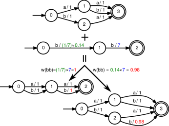
Figure 3: Exact arithmetic can reduce WFSM size. We consider the union of two WFSMs with exact and inexact representation of weights. With exact arithmetic, the path for $bb$ contains the weights $\frac{1}{7}$ and $7$, resulting in the path weight $w(bb)=\frac{1}{7}\times 7=1$. Since the union of the two WFSMs contains the strings $\{a,b\}^{2}$ with weight 1 each, it can be minimized to a small WFSM (bottom left). However, in the inexact representation (decimal with two significant digits), the path weight becomes $w(bb)=0.14\times 7=0.98$, which cannot be merged with the existing path of weight 1, generating one extra state and two extra transitions.

Typical solutions for this problem with floats is to quantize them or to test for approximate equality rather than exact equality, both of which are applied in OpenFST. However, these strategies are ultimately unsuccessful at preventing error accumulation when many repeated WFSM operations are performed, as necessary in Algorithms 1 and 2. This is no minor issue; the accumulation of inaccuracies led to an explosion of WFSM size that prevented us from doing any testing on real data.

To illustrate this issue, consider the problem of computing $M=\sum_{i}M_{i}$, where each $M_{i}$ contains one string in $S=\{0,1,2\}^{6}$ with unit weight. The different $M_{i}$ are all disjoint and their union is all of $S$. Therefore, $w_{M}(s)=1$ for all $s\in S$, making this essentially an unweighted FSM with a minimal $M$ of 7 states and 18 transitions. In Figure 4, we show how WFSM size grows with the number of strings contained in intermediate stages of computing $M$. An unweighted FSM implementation indeed contains 7 states and 18 transitions, whereas a WFSM implemented with float weights produces a “minimal” $M$ with 80 states and 237 transitions.

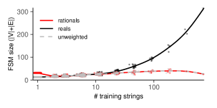
Figure 4: Exact rational arithmetic can prevent state explosion when merging many WFSMs. A WFSM representing all strings in $\{0,1,2\}^{6}$ is constructed by successively merging single-string FSMs in a binary tree recursion. With unweighted FSMs, shared substrings are exploited at every stage yielding a strongly compressed FSM. With real-weighted FSMs, even though all weights are initially the same, inaccuracies accumulate and prevent states from being merged (black line). Using exact rational arithmetic prevents this issue and rescues the desired behavior, leading to the same final result as in the unweighted case (red line). Points show FSM sizes for different numbers of training strings (with some jitter added in the x-direction to avoid overplotting). Lines show a Loess smoothing of the data.

To address these issues, we implementeded weights using an exact rational representation from Boost [3], which restored the equivalence with the unweighted FSM in the final output, and where intermediate stages were at most four times larger.

4 Empirical analysis

Standard non-weighted repertoire models were based on the assumption that the universe $\mathcal{U}$ of elements to be classified is disjointly partitioned into “self” and “nonself” subsets, and the goal was to estimate the boundary between these two classes [10, 19]. In theory, such problems be perfectly solved without taking the multiplicity of input strings into account: a single witness string is enough to perfectly decide membership.

Unfortunately, many real-world problems do not fit this assumption. For example, suppose we were to distinguish language based on n-grams (short sequences of letters). It is known that even short n-grams such as 3-grams contain enough information to solve this task satisfactorily [6]. However, given enough input text, almost every combination of 3 input letters will likely occur at least once in the input regardless of the language (it has been pointed out that llj is not a typical letter sequence in English but “only a killjoy would claim” it never occurs [6]). This should make it critical to not only consider the presence or absence of a string, but also its frequency. Interestingly, previous research has shown that negative selection algorithms can nevertheless solve such problems reasonably well [21]. However, the amount of input text used in these studies was relatively small.

One way to model the aforementioned type of classification problems is by considering a “fuzzy membership function” $f:x\mapsto[0,1]$ that assigns a degree of membership of each string to every class. Despite existing results on the negative selection problem, we hypothesized that unweighted AIS should perform poorly on such fuzzy problems.

4.1 The noisy bitstring problem

To test our hypothesis, we first defined a very simple toy example of a fuzzy classification problem. In this noisy bitstring problem, we consider random bitstrings $X(c,\mu)$ where $c\in\{0,1\}^{\ell}$ and $0\leq\mu\leq 1$. $X(c,\mu)$ is generated by the following algorithm: draw a random number $x$ from a geometric distribution with parameter $1-\mu$. Let $x^{\prime}=\min(x,\ell)$. Flip $x^{\prime}$ randomly chosen bits of $c$ and return the result. In particular, $X(c,0)$ is always $c$, and $X(c,1)$ is always the bitwise complement of $c$.

We can set up a fuzzy classification problem by defining the following membership functions $f_{0}$ and $f_{1}$:

$$f_{0}(x)=\text{Prob}(X(0^{\ell},\mu)=x);f_{1}(x)=\text{Prob}(X(1^{\ell},\mu)=x)$$

Particularly, for $0<\mu<1$, every bitstring has a nonzero probability of occurrence in both $X(c,0)$ and $X(c,1)$, but for $\mu\ll 1$, we have for example that $f_{0}(0^{\ell})\gg f_{1}(0^{\ell})$. Our repertoire $D$ is now tasked with assigning a score $D(t)$ to every string such that the distributions $D(X(0^{\ell},\mu))$ and $D(X(1^{\ell},\mu))$ are as different as possible – we will use the AUC metric to measure this difference.

To solve this problem, it should be critical to take multiplicity into account.

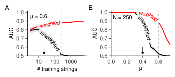
Figure 5: Positive selection poorly classifies noisy bitstrings for large inputs, but can be rescued by adding weights. A: AUC (mean $\pm$ SEM) of 20 independent runs, using $\ell=8,\mu=0.6$ and $5$-contiguous matching, varying input sizes N, and a test set of 100 random samples per class. B: likewise, but for a fixed training set size of 250 strings, now varying the mutation rate $\mu$. Dashed lines represent the same parameter combination with $N=250,\mu=0.6$. Arrows represent the values of $\mu$ and $N$ for which the expected number of strings with a majority of foreign bits in a training sample exceeds 1.

When simulating unweighted versions of positive selection, we found the seemingly paradoxical effect that performance was reasonable for small input samples, but then rapidly degraded for larger input samples (Figure 5A, black line). This occurred because with larger samples it became more and more likely to find the center string of the “foreign” class in the input. By contrast, weighted positive selection should not be “fooled” by such rare events because it can also learn from the frequencies of patterns in the input strings. Indeed, while multiplicity in the training set is rare for small samples and the two versions initially behaved very similarly, the performance of weighted selection kept improving with larger samples as expected (Figure 5A, red line). Thus, we can indeed conclude that fuzzy classification problems can be difficult to solve using unweighted repertoire models, especially at large sample sizes. Weighted positive selection was also more robust to higher mutation rates $\mu$ (Figure 5B), which – similar to larger input sizes – endanger performance by increasing the frequency of foreign-looking strings in the training input.

A well-known problem with repertoire models is their sometimes extreme sensitivity to the threshold parameter $t$ that determines when strings appear as “similar” to the receptor repertoire [5, 4, 16, 21]. We also found this effect for unweighted positive selection on noisy bitstrings, where the “best” $t$ additionally depended on input size (Figure 6A). Interestingly, we found that weighted positive selection was more robust to the choice of $t$, with $t=2,3,4$ now giving very similar performances throughout a range of input sizes (Figure 6B).

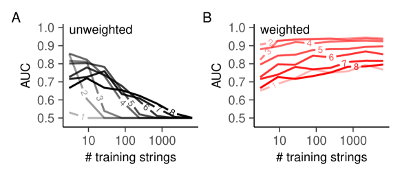
Figure 6: Weighted positive selection (A) is less sensitive to the threshold parameter $t$ than unweighted positive selection (B). AUCs (mean $\pm$ SEM) are shown for 20 independent runs, using $n=8,\mu=0.6$ and contiguous matching with varying thresholds $t$ (colored lines). Training and test sets were generated as in Figure 5.

These results suggest that on fuzzy classification problems, our weighted WFSM-AISs outperform their unweighted counterparts and are less sensitive to parameters like input size and detection threshold. The question remains: was this an extreme example, or does the same apply to real-world datasets?

4.2 Language anomaly detection

We therefore revisited the problem of language anomaly detection as considered previously [21]. In that study, repertoires selected on English strings could detect test strings from “anomalous“ languages among English strings reasonably well. However, the training sets used were relatively small ($<1000$ English strings, using contiguous matching with $t=3$) – small enough that foreign-looking 3-grams are unlikely to appear in the training data. We therefore asked: would the performance of such an (unweighted) AIS degrade as “unlikely” letter patterns do start to appear among English training strings?

To test this hypothesis, we downloaded the published set of strings from [21], as well as $\sim$800,000 English strings from the King James bible for training. From these data, we extracted 3-letter strings, and used our WFSM-AIS to perform both weighted and unweighted positive selection on randomly sampled inputs of up to 50,000 English training strings. When detecting Latin among English strings, we found that weighted positive selection once again started to outperform its unweighted counterpart at large input sizes (Figure 7).

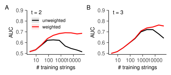
Figure 7: Language anomaly detection performance of a positive selection algorithm drops for large training sets and is rescued by adding weights. 3-grams were extracted from Latin or English strings, and (un)weighted positive selection performed with $t$-contiguous matching against English strings for either $t=2$ (A) or $t=3$ (B). Plots show the AUC (mean $\pm$ SEM) of 20 independent runs.

The input size where unweighted selection starts to perform badly depended on the threshold $t$; unlikely 2-grams might appear even in relatively small training sets of $\sim$100 strings, whereas the most unlikely 3-grams are rare enough that they do not appear in training sets of up to $\sim$1000 strings. Nevertheless, even these rare patterns eventually caused the performances of the weighted and unweighted AISs to diverge as inputs reach a size of several thousands of strings (Figure 7). Similar results were observed when substituting different languages for the anomalous strings (Figure 8). The size of the effect depended on the general similarity between English and the “anomalous” language considered – in line with the intuition that adding weights should not help learn a difference that is not there (e.g., in the case comparing English versus more English or medieval English).

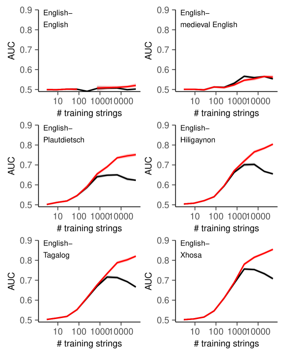
Figure 8: Analysis of Figure 7 performed for different languages. English-English is a negative control experiment where both “normal” and “anomalous” test strings are taken from the same language. Plots show the average AUC of 20 independent runs with $t=3$, comparable to Figure 7B.

All in all, our results demonstrate that when anomalous inputs have a non-zero probability to appear among training data, unweighted AISs perform poorly as the training set size increases. By contrast, weighted AISs are able to circumvent this issue by learning the information contained in the multiplicity in the training data. These findings suggest that weights will be crucial when applying AISs to real-world datasets.

5 Future work

Our experiments with WFSM-AISs revealed two key issues which we feel will be important to address in future work. First, building a WFSM-AIS in our current framework requires merging very large numbers of small classifiers. The OpenFST framework we currently use implements WFSM union in a way that does not yield a minimal result, such that we need to call minimization after every union to keep FSM size manageable. For unweighted FSMs with a “levelled” structure that repertoire models typically use (i.e., acyclic FSMs where all paths between two nodes have the same length), Textor et al. [18] implemented a custom FSM union algorithm that directly outputs a minimal FSM. This could be extended to WFSMs in future work. Likewise, we could use a directly determinizing union algorithm like the one by Mohri [13], created for a similar use-case. Minimization may also be sped up by the algorithm by Eisner [7].

Second, handling weights in WFSMs proved to be more challenging than one might perhaps anticipate. Our use of exact rational algebra proved critical to get our WFSM-AISs to work even on small input samples – without it, even repertoires trained on as few as 1000 input characters could rapidly blow up to 100s of megabytes in size. While the use of rationals greatly improved this and allowed us to perform the experiments reported in this paper, it is not a complete solution because the rationals themselves may “blow up” and use numerators or denominators that are too large to be represented as integers. In such cases quantization becomes necessary, bringing back the issue that strings with equal weights may no longer be recognized as such. While this did not cause any major issues in the experiments reported in this paper, we expect it to become problematic when storing large numbers of strings with very different weights at very different orders of magnitude. Further research is required to develop techniques to recognize such issues, understand the worst-case impact, and mitigate the effect. Since WFSMs are generic data structures that are used in many different fields, such research may be useful outside of the AIS context.

6 Conclusion

AIS were originally invented in the 1990s, a time in which modern ML/AI technology did not yet exist, and anomaly detection problems – especially sequence-based ones – were hard to solve. Nowadays with sequence-based end-to-end learning and transformers, anomaly detection in sequence data can be approached using state-of-the-art neural network models. Such models can scale to millions or billions of parameters to learn semantic features of large sequence datasets. Despite our contributions in this paper, AIS models are not yet optimized anywhere nearly as well. Crucially, such approaches are gradient-based, whereas AIS remains essentially a grandient-free approach. Even before all this, Stibor wrote already in 2006 that (negative selection) “was thoroughly explored” and that “future work in this direction is not meaningful” [15]. Why, then, still bother with AIS?

We do agree that AIS is unlikely to become a competitive technology for anomaly detection in sequence data anytime soon. We disagree, however, that AIS has been “thoroughly explored”. For example, our simple experiments with noisy classification problems in Section 4 have revealed a new fundamental issue with the decades-old negative selection algorithm : its performance degrades when the input data becomes too large. This fundamental issue has (to our knowledge) never been pointed out before, possibly because without FSM-based AISs, it has not been possible to build systems of the scale required to even allow processing of inputs of this size. This shows how we need to build such systems at scale to fully understand their properties.

Currently, the most important motivation to carry out this work is to study the information processing capacity of the immune system itself, which remains incompletely understood. For example, recent data cast substantial doubt on the long-standing immunological theory of negative selection, which the eponymous algorithm is based on. Repertoire models have been instrumental to place these new findings into context and to develop a more fine-grained understanding of the function of selection processes in the thymus. Again, such models need to be large-scale to be useful, because real immune systems contain many millions to billions of cells.

Beyond computational immunology, we are intrigued by the fact that the close similarity of AIS repertoire models and learning classifier systems (LCS) has not been explored further. LCS have similar issues as AIS around scale and (doubts about) usefulness, although LCS are typically used in a reinforcement learning setting where the ability to process very large sets of input data is not immediately critical. While the AISs we considered in this paper focused mostly on the initial stages of repertoire development – positive and negative selection – the processes occurring throughout an individual’s lifetime are more akin to reinforcement learning: pathogens are recognized, eliminated and memorized through an evolution-like process, which in the case of B cells also involves mutation of the repertoire sequence and fitness-based selection (affinity maturation). Therefore, we feel that (repertoire-based) AISs should ultimately be seen as a special case of LCS. We hypothesize that the WFSM framework developed in this paper should be equally useable to increase the scale of LCS such that richer, more interesting problems can be studied. We hope that the insights gleaned from such work will allow us to better understand parallel distributed information processing systems in Nature, including but not limited to the immune system.

References

- [1] Cyril Allauzen et al. “OpenFst: A general and efficient weighted finite-state transducer library” In International Conference on Implementation and Application of Automata, 2007, pp. 11–23 Springer
- [2] Joseph N. Blattman et al. “Estimating the Precursor Frequency of Naive Antigen-specific CD8 T Cells” In Journal of Experimental Medicine 195.5 Rockefeller University Press, 2002, pp. 657–664 DOI: 10.1084/jem.20001021
- [3] Boost “Boost C++ libraries”, https://www.boost.org/
- [4] P. D’haeseleer “An immunological approach to change detection: theoretical results” In Proceedings 9th IEEE Computer Security Foundations Workshop IEEE Comput. Soc. Press, 1996 DOI: 10.1109/csfw.1996.503687
- [5] P. D’haeseleer, S. Forrest and P. Helman “An immunological approach to change detection: algorithms, analysis and implications” In Proceedings 1996 IEEE Symposium on Security and Privacy IEEE Comput. Soc. Press, 1996 DOI: 10.1109/secpri.1996.502674
- [6] Ted Dunning “Statistical Identification of Language”, 1994
- [7] Jason Eisner “Simpler and more general minimization for weighted finite-state automata” In Proceedings of the 2003 Human Language Technology Conference of the North American Chapter of the Association for Computational Linguistics, 2003, pp. 64–71
- [8] Michael Elberfeld and Johannes Textor “Negative Selection Algorithms on Strings with Efficient Training and Linear-Time Classification” In Theoretical Computer Science 412, 2011, pp. 534–542 DOI: 10.1016/j.tcs.2010.09.022
- [9] Yuval Elhanati et al. “Quantifying selection in immune receptor repertoires” In Proceedings of the National Academy of Sciences 111.27 Proceedings of the National Academy of Sciences, 2014, pp. 9875–9880 DOI: 10.1073/pnas.1409572111
- [10] S. Forrest, A.S. Perelson, L. Allen and R. Cherukuri “Self-nonself discrimination in a computer” In Proceedings of 1994 IEEE Computer Society Symposium on Research in Security and Privacy IEEE Comput. Soc. Press, 1994 DOI: 10.1109/risp.1994.296580
- [11] Stephanie Forrest and Alan S. Perelson “Genetic algorithms and the immune system” In Parallel Problem Solving from Nature. PPSN 1990, Lecture Notes in Computer Science Springer-Verlag, 1990, pp. 319–325 DOI: 10.1007/bfb0029771
- [12] Maciej Liśkiewicz and Johannes Textor “Negative Selection Algorithms Without Generating Detectors” In Proceedings of Genetic and Evolutionary Computation Conference (GECCO 2010) ACM, 2010, pp. 1047–1054 DOI: 10.1145/1830483.1830673
- [13] Mehryar Mohri “On some applications of finite-state automata theory to natural language processing” In Natural Language Engineering 2.1 Cambridge University Press, 1996, pp. 61–80
- [14] J K Percus, O E Percus and A S Perelson “Predicting the size of the T-cell receptor and antibody combining region from consideration of efficient self-nonself discrimination.” In Proceedings of the National Academy of Sciences 90.5 Proceedings of the National Academy of Sciences, 1993, pp. 1691–1695 DOI: 10.1073/pnas.90.5.1691
- [15] Thomas Stibor “On the Appropriateness of Negative Selection for Anomaly Detection and Network Intrusion Detection”, 2006
- [16] Thomas Stibor, Philipp Mohr, Jonathan Timmis and Claudia Eckert “Is negative selection appropriate for anomaly detection?” In Proceedings of the 7th annual conference on Genetic and evolutionary computation ACM, 2005 DOI: 10.1145/1068009.1068061
- [17] Johannes Textor “A Comparative Study of Negative Selection Based Anomaly Detection in Sequence Data” In Proceedings of the 11th International Conference on Artificial Immune Systems (ICARIS ’12) 7597, Lecture Notes in Computer Science Springer, 2012, pp. 28–41 DOI: 10.1007/978-3-642-33757-4“˙3
- [18] Johannes Textor, Katharina Dannenberg and Macie Liśkiewicz “A generic finite automata based approach to implementing lymphocyte repertoire models” In Proceedings of the 2014 Annual Conference on Genetic and Evolutionary Computation, 2014, pp. 129–136
- [19] J. Timmis, A. Hone, T. Stibor and E. Clark “Theoretical advances in artificial immune systems” In Theoretical Computer Science 403.1 Elsevier BV, 2008, pp. 11–32 DOI: 10.1016/j.tcs.2008.02.011
- [20] Stewart W. Wilson “ZCS: A Zeroth Level Classifier System” In Evolutionary Computation 2.1 MIT Press - Journals, 1994, pp. 1–18 DOI: 10.1162/evco.1994.2.1.1
- [21] Inge MN Wortel et al. “Is T Cell Negative Selection a Learning Algorithm?” In Cells 9.3 MDPI, 2020, pp. 690
- [22] Veronika I. Zarnitsyna et al. “Estimating the Diversity, Completeness, and Cross-Reactivity of the T Cell Repertoire” In Frontiers in Immunology 4 Frontiers Media SA, 2013 DOI: 10.3389/fimmu.2013.00485