On Data-Driven Modeling and Control in Modern Power Grids Stability: Survey and Perspective

Abstract

Modern power grids are fast evolving with the increasing volatile renewable generation, distributed energy resources (DERs) and time-varying operating conditions. The DERs include rooftop photovoltaic (PV), small wind turbines, energy storages, flexible loads, electric vehicles (EVs), etc. The grid control is confronted with low inertia, uncertainty and nonlinearity that challenge the operation security, efficacy and efficiency. The ongoing digitization of power grids provides opportunities to address the challenges with data-driven and control. This paper provides a comprehensive review of emerging data-driven dynamical modeling and control methods and their various applications in power grid. Future trends are also discussed based on advances in data-driven control.

1 Introduction

Renewable energy is replacing fuel-type generation for sustainable power grids, aiming to reduce greenhouse gas emissions [1]. The modern power grids are composed of diverse energy resources interconnected through power networks, which include centralized energy resources (e.g., synchronous generators, solar and wind farms), and distributed energy resources (DERs) (e.g., distributed renewable generation, energy storage systems, electric vehicles, and thermostatically controlled loads). Particularly, many modernized energy resources are power converter-interfaced and “low-inertia” in nature. The uncertainty and nonlinearity of them endanger grid operation security, efficacy and efficiency [1, 2].

The uncertainty and nonlinearity of modern power grids originate from both the energy resources and their systemwide interactions. First, the rapid growth of renewable energy and flexible loads introduces uncertainty and nonlinearity due to the nonlinear stochastic nature of the renewable sources (e.g., wind and solar) and the human behaviors[2]. Second, the interaction dynamics of energy resources through the power networks could suffer from nonlinearity when encountering large disturbances. Besides, the increasing number of diverse energy resources and their hierarchical multi-timescale operation increases the system complexity. All these factors pose challenges to acquiring accurate system dynamic models and maintaining stable and secure operation of power systems.

Fortunately, the ongoing digitization (e.g., the fast-deploying information, communication and computing techniques) throughout power grids provides opportunities to address the operational challenges by data-driven control. In this paper, we consider the hierarchical control framework as it is the mature and scalable means to aggregate and manage massive energy resources in modernized power grids [3, 4, 5]. From the bottom to top of the hierarchical structure are distributed energy resources, microgrids/virtual power plants/centralized energy resource, and system operators. The hierarchical control includes primary control at the individual DER level, and secondary and tertiary control at the systemwide level. Examples of the control functions for different control types are summarized in Table 1.

Table 1: Examples of control functions for different control types

Type of Control	Functions
	Voltage/frequency stability perseverance,
Primary (Component)	plug-and-play of DERs,
	inertia and local damping control.
	Voltage restoration/regulation,
Secondary (Area)	wide-area damping control,
	frequency regulation.
	Energy management,
Tertiary (Grid)	optimal operation,
	tie-line power flow control.

With the data from the advanced sensing infrastructure (e.g., sensors or transducers, phasor measurement units, smart meters), the energy resources can be coordinately controlled to realize different operation objectives at different levels and time scales in a model-free data-driven fashion. To lift the operational challenges, effort has been made to apply data-driven control methods for different use cases in modern power grids and microgrids, such as voltage control [6, 7, 8, 9, 10], frequency control [11, 12, 13, 8, 9, 10, 14], wide-area damping control [15, 16, 17], cyber-resilient control [12, 18, 19, 14], as well as demand response [20, 21, 22, 23]. From the high-level perspective, the data-driven control methods in these studies are based on surrogate models which can be classified into: (1) linear system data-driven control methods; (2) nonlinear system data-driven control methods. This paper provides a comprehensive review on the recent advances of both categories of the methods, with the concentration on the second category that can be further classified into: (2.A) pure machine learning-based methods; (2.B) physics-informed machine learning methods; (2.C) Koopman-based methods. Besides, the paper will discuss the existing applications and trends of these methods in modern power grids.

Note that emerging data-driven methods such as iterative feedback tuning, model-free adaptive control, and learning-based control are hot topics and reviewed by the researchers in control and robotics communities [24, 25, 26, 27]. For example, the learning-based model-predictive control [26] was investigated for best closed-loop performance through either improved prediction model or proper parameterization of controller (costs and constraints). The mathematical formulation of learning-based control and reinforcement learning (RL) were also discussed based on different safety levels [27]. However, these review papers did not particularly focus on power system applications. The papers [2, 28] summarized data-driven control in modern power grids, whereas they mainly focused only on the category (2.A) mentioned above, i.e., universal machine learning methods such as RL. The review paper [29] was the first comprehensive summary of current microgrid control framework with applications of RL to address emerging microgrid challenges (i.e., uncertainty and extreme weather). It illustrated the fusion of RL in three ways: (i) model identification and parameter tuning; (ii) supplementary signal generation; (iii) controller substitution. However, the focus of [29] was still pure RL that belongs to the category (2.A); the data-driven yet interpretable modeling (with control inputs incorporated) was not illustrated. Besides, emerging data-driven control frameworks other than RL were not investigated. The review paper [30] presented a comprehensive investigation of physics-informed neural network (NN) for power system applications, which fell in the category (2.B) whereas the review concerned only a specific learning machine (i.e., NN) and the incorporation of control was not discussed in detail.

Motivated by the limitations of previous review papers, the goal of this paper is to provide a comprehensive method review of data-driven approaches with a broader scope, aiming to address increasing time-varying uncertainty and nonlinearity in modern power grids. It is important to note that data-driven control methods are not intended to replace existing model-based control frameworks [29], but rather to complement them as supplementary or enhancement solutions driven by data. By offering a broader technology map and comparative vision of different data-driven control approaches, this paper aims to inspire new ideas and feasible solutions in power systems. Compared to previous review works [28, 2, 30], this paper makes the following key contributions:

(1) It includes a broader range of methods, encompassing linear identification and control techniques based on input-output models, state space representations, transfer function identification, as well as nonlinear methods such as reinforcement learning, supervised learning-based and Koopman-based approaches.

(2) It provides a comprehensive comparison of data-driven approaches from various perspectives, including modeling structure, identification and control methods, data requirements, adaptiveness, interpretability, scalability, and training efficiency. Particularly, this paper introduces a notable advancement by including and reviewing Koopman-based methods for the first time. These methods are categorized as (2.C) and are particularly promising in addressing challenges such as nonlinearity and uncertainty while leveraging established linear identification and control techniques in conjunction with emerging machine learning methodologies.

(3) The paper organizes different categories of data-driven methods systematically to generalize the data-driven control frameworks, enabling researchers and practitioners to navigate through the diverse landscape of data-driven approaches in a more systematic manner, fostering novel ideas and feasible data-driven solutions in power systems.

The rest of this paper is organized as follows. Section 2 presents the preliminaries and a brief history of state-of-the-art data-driven control methods in power grid applications. Sections 3-4 present critical reviews for both categories of data-driven methods. Specifically, Section 3 elaborates on the linear system data-driven control methods. Section 4 details nonlinear system data-driven control methods. Section 5 provides a grid application overview and discusses the future trend. Section 6 concludes the paper.

2 Preliminaries and an Overview on Data-Driven Control for Power System Applications

This section presents an overview of data-driven identification and control methods and their applications in power systems. First of all, the following terminologies adopted in the manuscript are synonyms of or highly related to data-driven control, thus they need to be clarified to avoid conceptual ambiguity.

1) Data-driven control: the term “data-driven” means that the identification and/or the design of the controller are based entirely on experimental data collected from the plant or simulators but not any explicit information from first principle mathematical models of the controlled process [25]. Data-driven control often refers to the closed-loop control starting and ending up with data [25]. In this paper, we focus on the data-driven control that is based on data-driven modeling, which is defined below.

2) Data-driven modeling: the modeling method based on identification or learning from data while disregarding explicit knowledge of the system’s physical behavior [31]. The modeling and identification/learning can be done with or without control inputs incorporated.

3) Model-free control: the “model” in model-free control and model-based control refers to the first principle physical model of the system of interest. The term “model-free” refers to an alternative technique to control systems without traditional first principle physical models. This can be done by using a simplified representation of the system in a data-driven fashion. In other words, it is a synonym for data-driven control [25].

4) Adaptive control: adaptive control is the control method used by a controller which must adapt to a controlled system with parameters which vary, or are initially uncertain [32]. The adaptive identification and control itself can be conducted based on either physical parametric models or data-driven models (model-free representations). Data-driven control may realize adaptiveness through online identification/learning that quickly adjusts the model parameters to achieve fast adaption to time-varying uncertainty.

According to the above-mentioned context: (i) Model-free control and data-driven control are mainly the same concepts that are interpreted from different perspectives of a method. Although certain physics-inspired information (such as structure design or constraints) may be incorporated in data-driven modeling and control, we assume model-free control and data-driven control are interchangeable terms in the manuscript. (ii) Data-driven control can be adaptive or not depending on whether online identification is realized. The two assumptions apply to the rest of the paper without further explanation.

Generally, the data-driven control methodologies can be classified by the assumed data-driven model, i.e., linear system control and nonlinear system control. In power system applications, the linear transfer function model and identification were first investigated since early-nineties to model the dynamical modes of power grids. An example is the transfer function of impulse response between small-signal inputs and outputs with least-squares identification presented in 1993 [33]. The identified transfer function can be applied for different purposes such as: (i) tuning, design, and testing of power system control systems such as power system stabilizer (PSS), static var compensator (SVC) and many others; (ii) validation of power system small-signal models for grid planning and operation. Different transfer functions can be identified to deal with different potential operating conditions, whereby robust controllers can be designed accordingly. In the meantime, the authors in [34] proposed a reduced-order linear state space model based on a minimal realization approach for modal analysis, which shows the effectiveness of linear methods identified by transient (sometimes termed as ring-down [35]) data for conventional power systems with large rotating masses. Similar work on multiple-input multiple-output (MIMO) state space identification based on pulses can be found in [36], which was effectively applied to the modal analysis of bulk power systems. The subspace methods including ORT, N4SID, MOESP, CVA) were used for the linear state space identification with different probing tests [36, 37, 38]. Afterwards, many variants of transfer function identification methods [39, 40, 41, 42, 43, 44, 45, 46, 47, 48, 13, 8] and state space identification methods [49, 50, 22, 51, 52, 15, 6] were developed for data-driven control in the context of power grid applications such as damping control, voltage control and microgrid control (primary, secondary and tertiary) and aggregated load control. Generally, both transfer function and linear state space methods can represent systems well using a locally linearized model around a fixed operating point under the assumption that the system is an LTI (linear time-invariant). However, modern grids tend to be low-inertia with the increasing penetration of volatile inverter-interfaced renewables, leading to wide-range dynamics with higher levels of time-varying uncertainty and nonlinearity. This compromises the LTI assumption. Also, the saturation of control signals and nonlinearity of control input channels can also undermine the LTI assumption, leading to a decrease in identification accuracy. The details of different linear identification and control methods will be discussed in Section 3.

Nonlinear identification methods are suited to address the above-mentioned challenges. Traditionally, nonlinear identification methods based on Hibert-Huang Transform (empirical mode decomposition + Hilbert analysis) are used to adaptively model power system nonlinear dynamics [35]. Supervised learning (i.e., a main branch of machine learning) based nonlinear modeling started emerging in the mid-nineties because of the more powerful nonlinear fitting capability of universal learning machines such as NNs [53, 54, 55, 56]. For example, in 1996, Innocent Kamwa et al [54] proposed a MIMO supervised-learning recurrent neural network (RNN) that is equivalent to a general differential equation, which can be trained offline with the output-layer parameters then identified online in a recursive fashion to adaptively describe time-varying nonlinear power system dynamics. However, supervised learning is more often used for nonlinear dynamic modeling without external control. To incorporate nonlinear control input channels in the modeling, adequate training data are necessary, which could be generated by actively probing test signals then collecting the response data for a long period of time. Such requirement is not practical as it is often not allowed to subjectively inject large signals into safety-critical systems like power grids, while probing low-level test signals may not sufficiently excite the system to obtain informative data.

Reinforcement learning (RL), as another branch of machine learning that inherently bridges control and mainly rely on offline simulators, becomes popular nowadays for the applications of data-driven control of power grids [2, 28, 29]. By interacting with the simulation environment to pursue Bellman optimality, the RL can yield optimized control policy that can be deployed. The control optimality is theoretically sound while without performance guarantee due to the existence of simulator uncertainty/modeling error and optimization error [57]. Combining RL with deep learning (i.e., deep reinforcement learning (DRL)) becomes popular to enhance mathematical optimality and generalization capacity of learning, and shows the effectiveness in power grid applications such as optimal voltage control [58], frequency regulation [59], EV charging scheduling [60], and battery management [61]. To improve the efficiency of deep learning , DRL may be developed under parallel computing frameworks which has been shown effective in autonomous voltage control and emergency control [62, 63, 64]. The details of pure machine learning-based identification and control methods, including supervised and reinforcement learning, will be provided in Section 4.1.

Although pure machine learning methods stated in the last two paragraphs are of full capacity to fit any nonlinearity, their practical applications in power systems face pressing challenges such as physical consistency, interpretability, generalization, safety, etc. Physics-informed rules and laws (physics-informed loss function, constraints, initialization, architecture design, hybrid and ensemble learning, etc.) become a growing consensus to mitigate the challenges [65]. The fusion of RL frameworks and physics-inspired information is another promising solution as it leverages the intrinsic connection between machine learning and control theories. The fusion can be conducted through catering the physics-informed rules and laws of supervised/unsupervised learning for RL in environment surrogate model, value function or policy design [65, 66, 67, 27]. However, further improvements are necessary to enhance structural interpretability and avoid physically inconsistent solutions, which could compromise data-driven control performance or even destabilize power grids. Additionally, machine learning based methods still face practical challenges in power grid applications, including data availability, training efficiency, scalability, and adaptiveness. [29]. The discussion about physics-informed machine learning-based methods will be given in Section 4.2.

The unsolved issues further motivate recent research works on adaptive Koopman operator control with online nonlinear identification [68, 69], aiming to adaptively map nonlinear control to linear control that works for both small and large signals. Specifically, the methods adopt small-signal linear space augmented with more physically interpretable nonlinear bases and are adaptively identified to address time-varying uncertainty. Although these methods are online and can be applied without warm-up training, Koopman state space is still determined empirically. Koopman generators that can estimate optimal and physical-consistent Koopman operators (based on physical states and control inputs) could be exploited with physics-informed learning and adequate offline data. The details of Koopman-based methods will be provided in Section 4.3.

In the following, we will concentrate on elaborating existing data-driven control methodologies in linear systems (Section 3) and nonlinear systems (Section 4) used in power grids. The overview of grid applications with these methods is provided in Section 5.

3 Linear System Identification and Control

In existing data-driven control methodologies for linear systems, identification and control are typically regarded as two tasks that are done in a sequential manner. Specifically, when the data of inputs and outputs (i.e., $\bm{u}_{d}$ and $\bm{y}_{d}$) are available, the identification of a model of interest $\bm{y}=\hat{\bm{y}}(\bm{x},\bm{u};\bm{\theta})$ for the unknown parameter $\bm{\theta}$ and state $\bm{x}$ can be written in a general form of minimizing a loss function $\mathcal{L}_{id}$ as below:

$$\bm{\hat{\theta}}=arg\min_{\bm{\theta},\bm{x}}\mathcal{L}_{id}(\bm{y}_{d},\hat{\bm{y}}(\bm{x},\bm{u}_{d};\bm{\theta}))$$ (1a)

$$\bm{x}\in\mathcal{X},\quad\hat{\bm{y}}\in\mathcal{Y}$$ (1b)

where $\mathcal{X}$ and $\mathcal{Y}$ are the state constraint set and the output constraint set, respectively. The control thereafter can be applied to the identified model with $\hat{\bm{\theta}}$, which is equivalent to the optimization in a general form of

$$\min_{\bm{u},\bm{x}}\mathcal{L}_{c}(\bm{y}_{r},\hat{\bm{y}}(\bm{x},\bm{u};\hat{\bm{\theta}}),\bm{x})$$ (2a)

$$\bm{u}\in\mathcal{U},\quad\bm{x}\in\mathcal{X},\quad\hat{\bm{y}}\in\mathcal{Y}$$ (2b)

where $\bm{y}_{r}$ is the reference output desired by control; $\mathcal{U}$ is the input constraint set; $\mathcal{L}_{c}$ is the loss function representing the control objectives in general.

Alternatively, the identification and control can be done simultaneously and directly with respect to the input $\bm{u}$ and output $\bm{y}$ while without the state $\bm{x}$. That is

$$\min_{\bm{\theta},\bm{u},\bm{y}}\{\mathcal{L}_{id}(\bm{y}_{d},\bm{u}_{d},{\bm{f}}(\bm{y},\bm{u};\bm{\theta}))+\alpha\mathcal{L}_{c}(\bm{y}_{r},{\bm{f}}(\bm{y,u;{\theta}}))\}$$ (3a)

$$\bm{u}\in\mathcal{U},\quad\hat{\bm{y}}\in\mathcal{Y}$$ (3b)

where $\alpha$ is the coefficient to weight the identification and control objectives in (3a). In short, the identification-control tasks in sequential and simultaneous fashions correspond to the indirect and direct data-driven control in the control community. Interested readers can refer to [70] for more theoretical details. In the following, we will discuss the indirect and direct linear system data-driven control methods in existing and potential power system applications, respectively.

3.1 Sequential Linear Identification and Control

For sequential identification and control, the identification plays an important role to realize effective modeling and thus control. In what follows, we focus on linear identification techniques that can be categorized as state space model-based and input-output model-based. The state space model is generally more suitable for multi-variable system modeling as it deals with the individual input/output variables in a vector space. Besides, intermediate states properly selected can help define the inherent input-output relationship when compared to the input-output “black-box” modeling based on transfer functions.

3.1.1 Linear System Identification Based on State Space Model

We consider a special form of the model representation $\hat{\bm{y}}(\bm{x},\bm{u};\bm{\theta})$ in (1a)

$$\bm{x}_{k+1}=\bm{A}\bm{x}_{k}+\bm{B}\bm{u}_{k}+\bm{\delta}_{k}$$ (4a)

$$\bm{y}_{k}=\bm{C}\bm{x}_{k}+\bm{D}\bm{u}_{k}+\bm{e}_{k}$$ (4b)

which is termed as the state-space model and has been widely used to represent power systems dynamics operating in ambient conditions. $\bm{A}$, $\bm{B}$ and $\bm{C}$ are the parameters corresponding to $\bm{\theta}$. $\bm{x}_{k}$ are the states of power systems (e.g., phasor angle, rotor angle, frequency, voltage), $\bm{y}_{k}$ are the observation outputs of power systems (e.g., frequency, voltage, power), and $\bm{u}_{k}$ are the control inputs (e.g., the reference power of generators). $\bm{\delta}_{k}$ and $\bm{e}_{k}$ are the process noise and the observation noise, respectively. The linear state space form is conducive to estimation, filtering, prediction and control. When system parameters are unknown, mature linear identification and control techniques can be used to apply on the system (4a)-(4b).

Given the system model in (4a)-(4b), classical linear identification can be applied to identify the parameters $A$, $B$, and $C$. Examples of classical linear system identification methods are subspace methods including CVA [71], N4SID[71, 72, 73, 49, 74, 51, 75, 76], MOESP [77, 72], OKID [78]. Generally, the data matrices with Hankel structure play an important role in these subspace methods because the signals (the input data, output data and the noises) in these algorithms are organized in the form of Hankel matrices [79, 80]. Specifically, let $\bm{U}_{P}$, $\bm{Y}_{P}$, $\bm{U}_{F}$ and $\bm{Y}_{F}$ represent the “past” input and output data, as well as the “future” input and output data, respectively. $[\bm{U}_{P},\bm{U}_{F}]^{T}$ constitutes the Hankel matrix of the input $\bm{u}$, and $[\bm{Y}_{P},\bm{Y}_{F}]^{T}$ constitutes the Hankel matrix of the output $\bm{y}$. The Hankel matrices with the depth of $L$ and trajectory length $T$ are as follows:

$$\begin{bmatrix}\bm{U}_{P}\\ -\\ \bm{U}_{F}\end{bmatrix}=\begin{bmatrix}\bm{u}_{0}&\bm{u}_{1}&...&\bm{u}_{T-L}\\ \bm{u}_{1}&\bm{u}_{2}&...&\bm{u}_{T-L+1}\\ \vdots&\vdots&\ddots&\vdots\\ \bm{u}_{L-1}&\bm{u}_{L}&\dots&\bm{u}_{T-1}\end{bmatrix}$$ (5a)

$$\begin{bmatrix}\bm{Y}_{P}\\ -\\ \bm{Y}_{F}\end{bmatrix}=\begin{bmatrix}\bm{y}_{0}&\bm{y}_{1}&...&\bm{y}_{T-L}\\ \bm{y}_{1}&\bm{y}_{2}&...&\bm{y}_{T-L+1}\\ \vdots&\vdots&\ddots&\vdots\\ \bm{y}_{L-1}&\bm{y}_{L}&\dots&\bm{y}_{T-1}\end{bmatrix}$$ (5b)

The data matrices can be arranged according to (4a)-(4b) as:

$$\bm{Y}_{P}=\bm{\mathcal{O}}_{L/2}\bm{X}_{P}+\bm{\mathcal{H}}_{L/2}\bm{U}_{P}$$ (6a)

$$\bm{Y}_{F}=\bm{\mathcal{O}}_{L/2}\bm{X}_{F}+\bm{\mathcal{H}}_{L/2}\bm{U}_{F}$$ (6b)

where $\bm{\mathcal{O}}_{L/2}=[\bm{C},\bm{CA},\dots,\bm{CA}^{\frac{L}{2}-1}]^{T}$ is the extended observability matrix; $\bm{H}_{L/2}$ is the lower Toeplitz matrix defined as:

$$\bm{\mathcal{H}}_{L/2}=\begin{bmatrix}\bm{D}&0&...&...&0\\ \bm{CB}&\bm{D}&...&...&0\\ \bm{CAB}&\bm{CB}&\bm{D}&...&0\\ \vdots&\vdots&&\ddots&\vdots\\ \bm{CA}^{\frac{L}{2}-2}\bm{B}&\bm{CA}^{\frac{L}{2}-3}\bm{B}&\dots&\bm{CB}&\bm{D}\end{bmatrix}$$ (7)

and $\bm{X}$ represents the sequence of the state vector with the length of $T-L+1$.

Then different subspace identification methods can be applied based on (6a)-(6b), which typically involve two steps: (a) identification of $\bm{\mathcal{O}}_{k}$ and $\bm{\mathcal{H}}_{k}$; (b) estimation of system parameter matrices (i.e., $\bm{A},\bm{B},\bm{C}$) from the identified $\bm{\mathcal{O}}_{k}$ and $\bm{\mathcal{H}}_{k}$ [72]. Detailed procedures and comprehensive comparisons of the subspace methods can be found in [79]. Besides, recursive stochastic subspace methods are also applied in power grid damping mode estimation and control to realize online adaptiveness [81, 82, 83].

Among the above-mentioned subspace methods, CVA [71, 84], N4SID [71, 72, 49, 73, 74, 51, 75], and MOESP [85] may have the bias problem in nature since they work under the open-loop assumption (i.e., control inputs $\bm{u}$ is not correlated to the process noise $\bm{\delta}$ and the observation noise $\bm{e}$). In contrast, the OKID (observer Kalman filter identification) and the variants are free of the bias problem even in the closed-loop condition that the control inputs $\bm{u}$ correlate $\bm{\delta}$ and $\bm{e}$. We refer readers to [79] for a detailed review of subspace methods, where the general procedure (including pre-estimation, regression or projection, model reduction and parameter estimation) is summarized. The above-mentioned classical identification is usually conducted with ambient data as the linearization is based on the assumption of small signals in ambient conditions. The efficacy of the identification may degrade during transients.

Once the state-space model is identified, mature linear control techniques can be applied. For example, different state-feedback control methods, such as linear quadratic regulator (LQR) and root locus-based control design, can be applied [49, 50, 51] for wide-area damping control. Model predictive control [85], root locus control design[75], residual-based control [82], and PID control [74] were also designed for damping control based on the identified models. The control parameters can be designed with heuristic optimization such as particle swarm optimization [74].

3.1.2 Linear System Identification Based on Input-Output Models

We consider another special form of the model representation, i.e., the transfer function-based model, which directly describes the time series of input $\bm{u}$ and output $\bm{y}$ as a “black-box” without the intermediate state $\bm{x}$ in (1a) and (2a). An example is the autoregressive moving average with external inputs (ARMAX) model:

$${A}(q)\bm{y}_{k}={B}(q)\bm{u}_{k-h}+{C}(q)\bm{\zeta}_{k}$$ (8)

$A(q)=1+a_{1}q^{-1}+a_{2}q^{-2}+\dots+a_{n_{a}}q^{-n_{a}}$ , $B(q)=b_{0}+b_{1}q^{-1}+b_{2}q^{-2}+\dots+b_{n-1}q^{-n+1}$ and $C(q)=1+c_{1}q^{-1}+c_{2}q^{-2}+\dots+c_{n_{c}}q^{-n_{c}}$ are the ARMAX polynomials; $q$ is the delay operator; the parameters $n_{a}$, $n_{b}$, and $n_{c}$ are the orders of the ARMAX model. $h$ is the time delay of the system and $1\leq h<n_{b}$. The term $\bm{\zeta}_{k}$ denotes the white-noise disturbance. Other types of transfer function-based models, such as output-error models and Box-Jenkin models, are illustrated in [86]. These models can be identified with prediction error methods, which aim to find the system parameters that minimize the prediction error [87, 88]. Fig. 1 shows a schematic structure of the prediction error method for a general input-output model, which tunes the model parameter $\theta$ to minimize the loss function of prediction error $\mathcal{L}$. Generally, the cost function can be defined as $\mathcal{L}=f_{c}(Q_{cov}(e_{p,k}))$, where $e_{p,k}=y_{k}-\hat{y}_{k}$ represents the prediction error; $f_{c}$ is a scalar monotonically increasing function; $Q_{cov}=\frac{1}{N_{sample}}\Sigma_{k=1}^{N_{sample}}(e_{p,k}e_{p,k}^{T})$ denotes the sample covariance matrix.

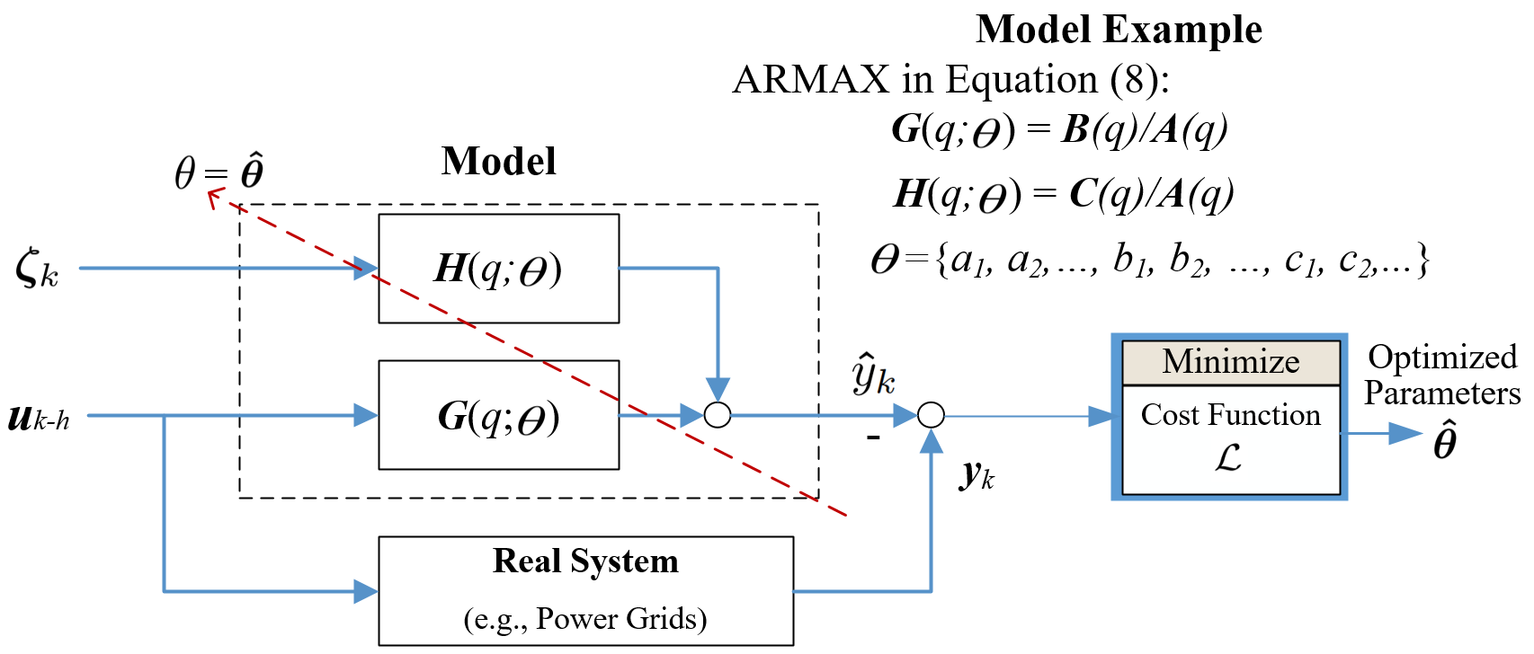
Figure 1: The schematic structure of prediction error methods.

For power system applications, the authors in [41] proposed an ARMAX-based damping control. The ARMAX was used to capture dominant inter-area modes of power systems identified in a least-squares fashion. Likewise, the authors in [44] assumed that the LVDC (low voltage direct current) system was linear and can be interpreted as a linear difference system equivalent to (8), which was identified with singular value decomposition. Another recently developed transfer function-based identification method was proposed in [89] based on the frequency response (FR) of multivariate continuous-time systems and convex optimization. This model-free method was applied to control battery energy storage systems in islanded microgrids to reduce voltage and frequency fluctuations [8]. The transfer function was identified in the spectral-analysis method [46], which applied the discrete Fourier transform to the auto-correlations of inputs and output data. The authors in [45] modeled the power system with continuous-time transfer functions too, which were identified online with ring-down data using a two-stage least-squares algorithm to realize the highest regression accuracy indices in both time domain and frequency domain.

Once the transfer function model is identified, classical control techniques, such as output-feedback control with lead-lag compensator [45] and networked predictive control [90], are applied for wide-area damping control. Generally, there is a trade-off between identification performance and robustness; a robust controller design is often favorable. For example, $H_{\infty}$ robust control has been applied in microgrid primary control [8]. A configuration information-free controller design for linear difference systems was also applied for active load stabilization in [44] based on a Lyapunov stability-oriented quadratic function and linear matrix inequality techniques. Similar LMI-based control can be found in [13], where some other goals such as power sharing and frequency/voltage restoration were incorporated in the objective function jointly with the stability requirements. In [48], an ARMAX model was identified whereby the estimate of inertia was obtained and sent to the local-area model predictive controllers to realize frequency regulation. Similar to 1), the input-output model is linear. Therefore, the identification is suitable for small signals in ambient conditions and usually conducted with ambient data. The efficacy of the identification may degrade during transients.

Another formulation of multi-input multi-output (MIMO) model is proposed in [91] based on a novel dynamic linearization technique. Specifically, the system of interest is adaptively linearized as:

$$\Delta\bm{y}_{k+1}=\bm{G}_{k}\Delta\bm{u}_{k}$$ (9)

$$\mbox{with }\bm{G}_{k}=\begin{bmatrix}G_{11,k}&G_{12,k}&...&G_{1p,k}\\ G_{21,k}&G_{22,k}&...&G_{2p,k}\\ \vdots&\vdots&\vdots&\vdots\\ G_{p1,k}&G_{p2,k}&...&G_{pp,k}\\ \end{bmatrix},\quad\|\bm{G}_{k}\|\leq b$$ (10)

where $b$ is a positive constant; $\bm{G}_{k}$ is the matrix of pseudo-partial derivative, which can be identified with time-varying parameter estimation algorithms such as modified projection [91], least squares with a forgetting factor [92], and the leakage recursive least-squares method [93]. Such a model has been used in the identification for microgrid primary control realizing a robust local voltage control that is not sensitive to the variations of the system parameter, structure, and control delay [47]. The model has also been used for power system stabilizers in [94] with improved dynamic performance for damping low-frequency oscillations under various operating conditions. Because the linearization is adaptive and the model can be identified in a rolling-based fashion, it can also handle nonlinearity and can be conducted for both ambient and transient data. However, the effectiveness based on transient data relies on the window length of data and the incurred inertia, which may hinder a timely model update.

3.1.3 Linear Identification Based on Ornstein-Uhlenbeck Process

The aforementioned identification techniques estimate the system parameters with minimized error in a mathematical sense while the mathematical solution is not unique. Therefore, the identified models may not reflect the real system state variables and the estimated parameters are not guaranteed to be the parameters of the true physical system, making the control design challenging. Leveraging the statistical properties of multivariate Ornstein-Uhlenbeck (OU) process, the data-driven identification methods developed in [6, 16, 15, 17] can estimate the system state matrix of the true physical model and extract modal properties and essential parameters. Assuming that the aggregated load powers experience Gaussian stochastic perturbations, the power system dynamic model in ambient conditions can be represented as

$$\bm{\dot{x}}=\bm{A}\bm{x}+\bm{B}_{P}\bm{\xi}$$ (11)

where the states $\bm{x}$ can be the deviations of generator rotor angle, generator rotor speed in wide-area damping control [16, 15, 17], or be the deviations of bus voltage magnitude and phase angle in wide-area voltage control [6] or load identifications [95]. $\bm{\xi}$ are mutually independent standard Gaussian random variables, representing the stochastic load variations; $\bm{B}_{P}$ is the noise intensity matrix. Thus, the state $\bm{x}$ in (11) follows a multivariate OU process. The parameter $\bm{A}$ corresponds to the Jacobian matrix of the true physical model containing significant information like all oscillation modes, mode shapes, participation factors, inertia and damping constants, dynamic load time constants, network topology parameters, etc.

The system parameter $\bm{A}$ can be analytically obtained by applying the regression theorem of OU process, which reflects the dynamical evolving of state covariances and relates the statistical properties of state variables with $\bm{A}$. Specifically,

$$\frac{d}{dt}\bm{G}(\tau)=\bm{A}\bm{G}(\tau),\mbox{with }\bm{G}(\tau)=<[\bm{x}(t+\tau)-\bar{\bm{x}}][\bm{x}(t)-\bar{\bm{x}}]^{T}>\\$$ (12)

Hence, $\bm{A}$ can be obtained uniquely and analytically by solving (12) according to [96]:

$$\bm{A}=\frac{1}{\tau}log[\bm{G}(\tau)\bm{G}(0)^{-1}]$$ (13)

Equation (13) tactfully provides a way to identify the true physical model $\bm{A}$ from the statistical properties of measurement data. Alternatively, $\bm{A}$ can be obtained based on the Lyapunov function that the stationary covariance matrix $\bm{G}(0)$ of multivariate OU process satisfies [15]:

$$\bm{A}\bm{G(0)}+\bm{G(0)}\bm{A}^{T}=-\bm{B}\bm{B}^{T}$$ (14)

if $\bm{B}$ is known. It was shown that the true system parameters were approximately obtained by using both identification methods (according to (13) and (14) respectively); then the identified model can be directly utilized in control design. Note that the OU-based methods are conducted with ambient data to identify the small-signal model of interest. Different from 3.1.1) and 3.1.2), this type of method can help obtain a unique identification solution that corresponds to the true physical small-signal model. Even though the model structure has certain physical interpretation, the methods are in nature “data-driven”.

Once the system of interest is identified by the methods stated above, conventional linear optimal or robust control methods can be applied. For example, modal linear quadratic regulators [17] and pole placement [16, 15] have been applied in wide-area damping control. Because the OU-based methods can identify the true system model, the wide-area damping controls designed based on the identified model can achieve full decoupling of modes and damp all critical modes simultaneously without affecting the others. Optimal control has also been applied in wide-area voltage control [6].

3.1.4 Loewner Method

Most of linear models and identification are based on a representation that can describe the system dynamics in the whole frequency range (e.g., the state space representation or transfer function input-output models). For a selective-frequency range, Loewner interpolation was commonly used in black-box modeling of large MIMO microwave structures that show the capability for rational interpolation of frequency data [97, 98]. In 2015, a tangential interpolation framework based on Loewner matrix pencil was first used in power systems for modeling frequency-dependent network equivalents that can describe electromagnetic transients (EMT) [39, 99]. In 2019, the Loewner interpolation method was used for the reduced-order model and identification for electro-mechanical models of multi-machine power systems [40]. The method can realize more accurate identification in a particular frequency range than other techniques. However, the Loewner methods are only suitable for linear time-invariant systems (i.e., assuming small signals at specific operating conditions), which may not hold for modern low-inertia power grids with increasing volatile renewables. Likewise, the identification based on Loewner method for a selective-frequency range was compared with the conventional eigensystem realization algorithm for a New-England 10-machine test system in 2020. The results show the performance enhancement in terms of the modal shape and the absolute error of identified frequency responses [43]. After applying Loewner methods, the identified transfer functions for different frequency ranges corresponding to different potential operating conditions then can be applied for robust controller design.

3.2 Direct Linear Identification and Control

Although the linear identification and control tasks are usually conducted sequentially as aforementioned, effort has been made to realize the two tasks simultaneously [70] to benefit the global optimality of joint identification and control. For example, data-enabled predictive control (DeePC) with quadratic regularization is investigated for local converter control [100]. It identifies the system parameters and designs control signals together by solving a single optimization problem of DeePC. In summary, the DeePC for the state space model (4a)-(4b) can be written in a generic form[101, 100]:

$$\min_{\bm{g},{\sigma}_{y},\bm{u},\bm{y}}\Sigma_{k=0}^{N-1}\|\bm{u}\|^{2}_{R}+\|\bm{y}-\bm{y}_{r}\|_{Q}^{2}+\lambda_{y}\|{\sigma}_{y}\|_{2}^{2}$$ (15a)

$$\mbox{subject to }[\bm{U_{P}},\bm{Y}_{P},\bm{U}_{F},\bm{Y}_{F}]^{T}g=[\bm{u}_{ini},\bm{y}_{ini}+\sigma_{y},\bm{u},\bm{y}]^{T}$$ (15b)

$$\bm{u}\in\mathcal{U},\quad\hat{\bm{y}}\in\mathcal{Y}$$ (15c)

where the operator $\|a\|_{X}^{2}$ denotes the quadratic form $a^{T}Xa$. $\lambda_{y}$ is the regularization parameter. ${\sigma}_{y}$ is an auxiliary slack variable to guarantee the feasibility of solving the optimization problem. $N$ is the prediction horizon. $\bm{u}_{ini}$ and $\bm{y}_{ini}$ are the most recent input and output trajectories of length $T_{ini}$.

The DeePC can be seen as a special form of (3a)-(3b), with $\bm{g}$ corresponding to the parameter $\theta$. The DeePC solves the convex optimization problem (15a)-(15c) in a receding horizon manner with a finite number of data samples to predict future trajectories. See details in [101]. The DeePC has been applied in modern power grids, such as local converter control [100], decentralized damping control [102], and frequency regulation [103]. The DeePC can also be used to guide the training phase of RL with improved sample efficiency, It was applied to load frequency control and the control performance was improved [104]. Another example of direct data-driven control is a multivariable linear parameter varying (LPV) controller applied in islanded microgrid secondary-primary control, resulting in damped oscillations in frequency and power dynamics [105]. Different from DeePC, the synthesis process is based on the frequency domain rather than the time domain.

It has been shown in the IEEE task force paper [35] that linearized models around the operating points can yield an approximation behaving at a reasonable level of accuracy using transient data and ambient data, respectively. Thus, the linear identification and control methods stated above, either indirect or direct, are still useful and credible in applications like electromechanical modes identification, dynamic load modeling, and wide-area damping control. Also, linear methods are advantageous in two respects: (i) their parameters can be identified optimally with the mature theory foundations of linear systems; (ii) it is easy to realize adaptiveness due to the parameter identification efficiency in linear models.

Nonetheless, linear system identification and control may still face challenges in power system applications: (i) Modern power grids, with the integration of increasing renewable energy sources, exhibit low inertia and fast-changing operating conditions subject to large disturbances, making the linear models inaccurate. (ii) The saturation of control signals and the diverse interactions between controllers may introduce nonlinearity and uncertainty, compromising identification accuracy and can even result in ineffective modeling [33].

4 Nonlinear System Identification and Control

To address the aforementioned complexity, uncertainty and nonlinearity of modern power grids, nonlinear data-driven control methods gain increasing attention. They are categorized as: (A) pure machine learning-based methods; (B) physics-informed machine learning; and (C) Koopman-based methods. Generally, the category (A) uses “black-box” machine learning to model nonlinear system dynamics and control. The category (B) intends to integrate physical information into the machine learning training or model structure design to realize more reliable modeling. The category (C) considers the Koopman operators to map nonlinear dynamics to linear state spaces, whereby mature linear control methods can be readily applied. The three categories are elaborated below.

4.1 Pure Machine Learning-Based Methods

Generally, machine learning includes reinforcement, supervised and unsupervised learning. Reinforcement learning, as a branch of machine learning that can bridge control, becomes popular nowadays for the applications of data-driven control of power grids [2, 28, 29]. The learning process generally depends on offline simulators to interact with rather than probing data to real systems to generate training data [2]. However, the RL training is often time-consuming, and the control performance rests on the simulator accuracy and the optimization error associated with highly nonlinear models.

Supervised learning can also be used for data-driven modeling for control. However, incorporating control input data in the supervised learning-based model, which is then used for control, is not popular because of data issues associated with control input channels. It is not feasible to probe large testing signals due to the practical operation requirements (especially for safety-critical systems like power grids). Even with low-level test signals, the closed control loops in power grids could trap the state-and-control pairs and make them ill-distributed [106], thus lacking rich information for universal learning machines such as NNs to generalize the impact from and to control input channels. In a sense, supervised learning is more often seen in power grid modeling without external control inputs rather than grid control applications. Details of the RL and supervised learning-based methods are provided in what follows.

Reinforcement learning (RL). RL is a branch of machine learning regarding how to learn control policies by interacting with the environment to explore and exploit inherent model structure according to Bellman optimality [57, 107]. In RL, the system states are assumed to evolve according to the Markov decision process (MDP), i.e., the probability of the system occurring in the current state is determined only by the previous state [57]. Specifically, an MDP consists of a set of states $s\in\mathcal{S}$, actions $a\in\mathcal{A}$, rewards $r\in\mathcal{R}$, the transition probability $Pr(s^{\prime},s,a)=Prob(s_{k+1}=s^{\prime}|s_{k}=s,a_{k}=a)$, and the policy function $\pi(s,a)=Prob(a_{k+1}=a|s_{k+1}=s)$. Thus, the state transition under the policy $\pi$ is

$$Pr(s^{\prime},s,\pi)=\Sigma_{a\in\mathcal{A}}\{\pi(s,a)Pr(s^{\prime},s,a)\}$$ (16)

The above MDP notation generalizes a Markov process to incorporate actions and rewards for RL, which can be used to describe any nonlinear system decision-making/control of interest. Fig. 2 shows the generic scheme of RL agent that learns the system through interaction with the environment (i.e., offline simulators), and then the learned agents are deployed to the real environment for online operation. Note that the RL agent can be either based on universal surrogate models (e.g., actor-critic with deep NNs, approximate dynamic programming, deep Q-learning, etc.), or uses purely model-free paradigms (e.g., Q-learning, SARSA, policy gradient, etc) [107, 57].

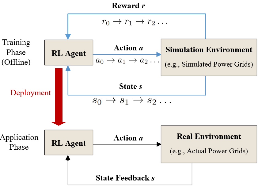
Figure 2: The schematic framework of RL.

In practical applications of power grids, Q-learning is among the most popular RL techniques [108, 109, 110, 111]. However, Q-learning is not inherently suitable for continuous action spaces [107]. In addition, the action and reward functions for RL are often unknown or of high uncertainty. Therefore, actor-critic methods gained attention [14, 59] and are favorable because of the iterative exploration and exploitation of the “actor” and “critic”. That being said, the action and reward functions are approximated with two separate learning machines (e.g., various NNs, and support vector machines), which are trained with abundant data. In a broader sense, such “actor-critic” can be seen as a direct data-driven control paradigm equivalent to (3a)-(3b) that identifies the system and generate control actions directly. However, the universal learning machines under the general RL framework often suffer from training efficacy and efficiency problems due to the unconstrained or loosely-constrained learning space: (a) the trained models may not well describe the underlying physical process well due to modeling error and training error; (b) the computational cost of training is high. The former issue can be mitigated by physics-informed techniques and Koopman-based methods that will be discussed in Sections 4.2-4.3. While the latter can be naturally lifted by parallel computing when applicable. For example, a wide variety of scenarios in power grids can be created in simulation to train DRL. For example, the authors in [62] parallelized training tasks based on environment study cases (e.g., fault scenarios in power grids). Furthermore, they proposed a two-layer parallel scheme [64] that supports task parallelism based on environment and learning parallelism based on a parallel augment random search algorithm, which was successfully applied in derivative-free DRL for emergency voltage control. It can realize well-structured and more effective parameter exploration (larger learning rates and fewer hyper-parameters to tune) than conventional action-space exploration in DRL, improving the computational scalability and accelerating the training (e.g., training time reduced by 136 times on the IEEE 300-bus system). Likewise, a parallel framework that employs multiple workers simultaneously interacting with power grid simulators was adopted for autonomous voltage control in [63], which shows improved training efficiency and stability.

As RL is a branch of mature machine learning techniques which have been well illustrated in many other works in the field of power systems, such as decentralized resilient secondary control [14, 108], microgrid frequency regulation[108, 59], microgrid power dispatch [112], reactive power control [58], battery management [60, 113, 61], multi-area AGC [114, 115], and wide-area damping control [116], they will not be detailed in this paper. Interested readers are referred to [2, 28, 29] for comprehensive reviews of RL in power system/microgrid applications.

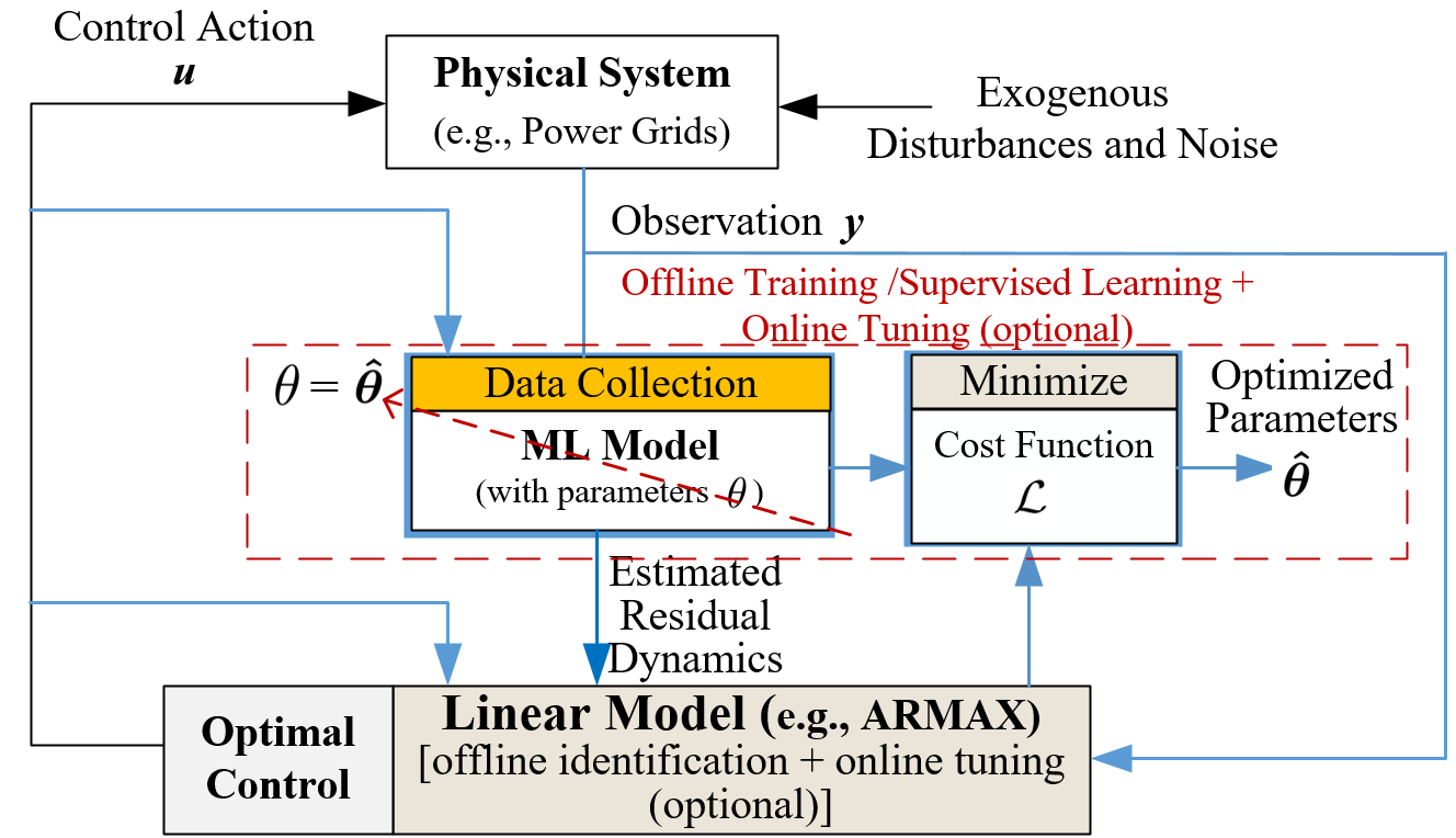
Figure 3: The schematic framework of supervised learning based modeling for control with a nonlinear learning machine and a linear model.

Supervised Learning-Based Method. Universal machine learning models, such as neural networks (NNs), can be used in power grids to model nonlinear dynamics [117]. For example, the authors in [7] used a linear dynamic model ARMAX to describe the microgrid voltage dynamics first and then trained NNs to compensate for the residual nonlinear dynamics on top of the linear model, whereby optimal control is applied to realize stabler and faster microgrid voltage control. Fig. 3 shows the schematic framework of supervised learning-based modeling for control with pure ML, where the learning machine is trained offline based on a user-defined cost function $\mathcal{L}$. Note that the linear model (e.g., ARMAX) may keep updating by online identification to realize fast adaptiveness. The ML model parameters may also be finely tuned online around the offline-trained model to realize a certain level of adaptiveness. This framework can be seen as a special form of the sequential data-driven control (1a)-(2b). It has been shown that the well-trained machine learning model can capture power system nonlinearity with supervised learning given abundant data [7, 118]. Besides the applications in power grids, the NN-based control is also used to model and control residual nonlinear dynamics of drone landing [119], where spectral normalization is used to stabilize NN training and to improve generalization capacity. Conventional loss functions for machine learning include root-mean-squared error, mean absolute error, cross-entropy, KL-divergence, etc, which can be used for different training algorithms such as Levenberg-Marquardt (LM) algorithm, stochastic gradient descent (with momentum) (SGD or SGDM), and adaptive moment estimation (ADAM) [57, 107].

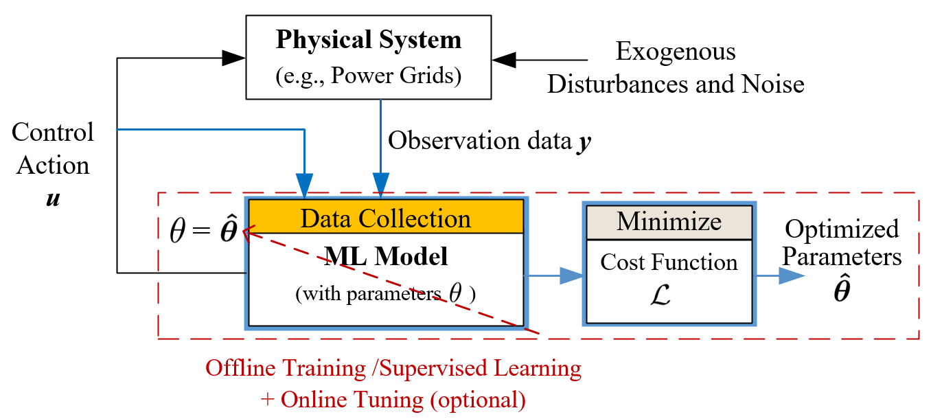
Figure 4: The schematic framework of supervised learning-based modeling for control with nonlinear learning machines only.

The learning machines can also be used to model the uncertainty of systems dynamics and then be directly used to regulate control signals as shown in Fig. 4. The offline-trained ML models may also be finely tuned with new online data to realize certain level of adaptiveness. Such an idea of offline pre-training and online-tuning matches the concept of transfer learning in machine learning community, which is a learning paradigm aiming to transfer the knowledge generalized from the data of existing systems to the learning of new similar systems by offline training and the learning machine parameters are fine-tuned when new data come [120]. This paradigm has been used in [10, 118, 121], where online-tuned NNs are used for identification and control to realize accurate power sharing and enhanced stability, respectively. The online tuning of NNs in [10, 118] can also be seen as a special form of the direct data-driven control (3a)-(3b), as the NNs are trained to model to obtain optimized parameters and to generate control signals simultaneously. NN-based control has also been used in a standalone DC microgrid where the NNs are trained offline to directly output desired control signals for individual converters of distributed energy resources to enhance microgrid voltage stability [122]. The optimal Koopman operators and the identification need further investigation.

Pure machine learning methods can be conducted with both ambient and transient data. However, the data should be informative enough to guarantee the generalization of learning machines. Besides, pure machine learning methods resolve the control policies as “black-boxes” with no explicit physical interpretation. Therefore, they are often analytically and computationally less tractable and less practical for real-time and safety-critical scenarios in power grids. Some physics-informed learning methods have been proposed to address the issues, which are presented as follows.

4.2 Physics-Informed Machine Learning Methods

The physics-informed machine learning can inform the learning machine of certain physics either through the training, the model structure design, or both. Thus, they can enhance the interpretability or explainability with more physics-consistent solutions. In what follows, we discuss physics-informed methods from the two perspectives. Interested readers are also referred to [65] for more detailed information regarding physics-informed NNs that have been used in power grids.

4.2.1 Physics-Informed Training

In the training phase of machine learning, different regularization and relaxation techniques[70, 123] can be incorporated to avoid over-fitting and increase physics interpretability. For example, different norms can be added in the regularization terms such that the system model complexity can be constrained under certain mathematical and physical interpretations (e.g., stability or other specific physical constraints). In general, the identification loss function with the regularization terms can be written as

$$\mathcal{L}_{id}= \mathcal{L}(\bm{y}_{d},\bm{\hat{y}}_{d})+\gamma\mathcal{L}_{P}(\bm{\theta})+\lambda\mathcal{L}_{Phy}(\bm{x},\bm{u},\hat{y})$$ (17)

where $\mathcal{L}$ is the conventional loss function that measures the distance between the predicted output and the target output. $\gamma$ and $\lambda$ are coefficients to weigh the regularization terms. $\mathcal{L}_{P}$ is the parametric regularization term (e.g., L1, L2, Tikhonov) to constrain the model complexity by regularizing the model parameters $\bm{\theta}$. $\mathcal{L}_{Phy}$ is the physics-informed regularization term to add extra physics-driven constraints. Alternatively, the physics-informed information can be added as the inequality and equality constraints $\mathcal{C}_{PhyIEQ}$ and $\mathcal{C}_{PhyEQ}$ as follows:

$$\mathcal{L}=\mathcal{L}(\bm{y}_{d},\bm{\hat{y}}_{d})+\gamma\mathcal{L}_{P}(\bm{\theta})$$ (18a)

$$\mathcal{C}_{PhyIEQ}(\bm{x,u,\hat{y}})\leq\bm{\zeta}$$ (18b)

$$\mathcal{C}_{PhyEQ}(\bm{x,u,\hat{y}})=\bm{\eta}$$ (18c)

where $\bm{\zeta}$ and $\bm{\eta}$ are arbitrary values to constrain the physics information.

The authors in [123] apply an adapted deep RL method with the training that is based on (18c) in wide-area damping control. The framework is called bounded exploratory control-based DDPG (deep deterministic policy gradient), consisting of NNs and polytopic controllers designed with the help of linear matrix inequality (LMI)-based mixed $H_{2}/H_{\infty}$ optimization. With the help of $H_{2}/H_{\infty}$-oriented stability physical constraints, the method is demonstrated effective for both low-stressed and high-stressed networks. Universal learning machines such as NN can be informed of physical ingredients in training. The authors in [124] use NN to realize a fast dynamic state and parameter estimation tool to assess power system stability. The cost function for NN training is in the form of (17), consisting of a physics-informed regularization term based on the swing equation with respect to the NN output. Similarly, the physics-informed NNs are used in [125] to capture the dynamics of power systems, with a group of state constraints and physics-informed differential and algebraic equation constraints incorporated in the NN architecture and loss functions equivalent to the form of (18c). The authors in [126] apply NN for high impedance fault detection in power grids. To obtain more reasonable NN parameters, an elliptical regularization term is added in the form of (17) to incorporate the physics-regulated elliptical characteristics of voltages and currents into the cost function for training. In summary, these physics-informed learning-based NNs show enhanced modeling efficacy and thus potentially beneficial for data-driven control on top of these NNs.

4.2.2 Physics-Informed Model Structure Design

The physics-informed training discussed in Section B intends to incorporate physical system information in the cost function $\mathcal{L}$, while the physical information can also be integrated into model structure design, i.e., “ML model” in Fig. 3-4. In fact, proper modeling with the physics-informed structure design can nail down the learning space within reasonable areas, which could make the modeling more reliable and the learning faster. Pure machine learning models as shown in Fig. 3 and Fig. 4 can be incorporated with certain levels of physics interpretations in the structure. For example, the authors in [30] proposed a physics-informed NN tailored by automatic differentiation [127] of the original NN, whereby power system physical laws (e.g., underlying swing equations) are incorporated with the bounded space of admissible solutions to the NN parameters [30]. It has been shown that the physics-informed neural nets can effectively describe the rotor angle and frequency for uncertain power inputs and identify system inertia and damping parameters. Such design also provides opportunities to lower the requirement on the sizes of NNs and the training data set. The physics-informed NN [128] that incorporates the regularization of power flow equations is proposed for power system state estimation under partial observability, achieving more accurate voltage-phasors estimation than conventional weighted least squares-based estimation. The authors in [129] proposed a hybrid learning structure by incorporating the physical AC power flow model into the deep learning with autoencoders. The authors in [130] use physics-informed NNs to accurately estimate the optimal power flow (OPF) with rigorous performance guarantee. The physical interpretation is further enhanced by adding the disparities of AC-OPF Karush–Kuhn–Tucker (KKT) condition to the NN training loss function. Additionally, the authors in [131] use physics-informed NN with an implicit Runge-Kutta integration [132] at the local converter level, whereby deep NNs and converter physical models are seamlessly coupled and reliable parameter estimation of power converters are achieved.

4.3 Koopman-Based Methods

As aforementioned in Section 2, data availability, training efficiency, interpretability, adaptiveness, and scalability issues further motivate recent research works on adaptive Koopman operator control [68, 69], aiming to adaptively map nonlinear control to linear control that works for both small and large signals. Koopman operator theory [133] shows that a nonlinear dynamical system can be transformed into an infinite-dimensional linear system under a Koopman embedding mapping. The Koopman-enabled linear model structure is a way to interpret nonlinear dynamics, and is valid for global nonlinearity with the infinite-dimensional representation as opposed to traditional locally linearized small-signal models. Practically, one can consider finite-dimensional Koopman invariant subspaces where dominant dynamics can be described. In Koopman-based data-driven control, the physics interpretation on power grids of interest can be incorporated through the model structure design. Particularly, given a nonlinear dynamical system with external control $\bm{x}_{k+1}=F(\bm{x}_{k},\bm{u}_{k})$, where $\bm{x}\in\mathcal{M}$ and $\bm{u}\in\mathcal{U}$ with $\mathcal{M}$ and $\mathcal{U}$ being the manifolds of state and control input, we consider the Koopman embedding mapping $\bm{\Phi}$ from the two manifolds to a new Hilbert space $\bm{\Phi}:\mathcal{M}\times\mathcal{U}\to\mathcal{H}$, which lies within the span of the eigenfunctions $\varphi_{j}$. That is, $\bm{\Phi(x,u)}=\sum_{j=1}^{N_{\varphi}}\varphi_{j}(\bm{\bm{x},\bm{u}})\bm{v}_{j}$, where $\bm{\Phi}(\bm{x},\bm{u})=[\Phi_{1}(\bm{x,u}),\Phi_{2}(\bm{x,u}),…,\Phi_{i}(\bm{x,u}),…,\Phi_{p}(\bm{x,u})]^{T}$ is a set of Koopman observables, $\bm{v}_{j}$ are the vector-valued coefficients called Koopman modes. The Koopman operator $\mathcal{K}$, acting on the span of $\varphi_{j}$, advances the embeddings $\bm{\Phi(x,u)}$ linearly in the Hilbert space $\mathcal{H}$ as [133]:

$$\bm{\Phi}(\bm{x}_{k+1},\bm{u}_{k+1}) =\mathcal{K}\Phi(\bm{x}_{k},\bm{u}_{k})$$ (19)

$$=\mathcal{K}\sum_{j=1}^{N_{\varphi}}\varphi_{j}({\bm{x},\bm{u}})\bm{v}_{j}=\sum_{j=1}^{N_{\varphi}}(\rho_{j}\varphi_{j}(\bm{x}_{k},\bm{u}_{k})\bm{v}_{j})$$

where $\rho_{j}$ are the eigenvalues satisfying $\mathcal{K}\varphi_{j}(\bm{x,u})=\rho_{j}\varphi_{j}(\bm{x,u})$. In (19), one can assume that $\Phi_{i}(\bm{x,u})=g_{i}(\bm{x})+l_{i}(\bm{u})$ where $g_{i}(\bm{x})$ is a nonlinear observable function and $l_{i}(\bm{u})$ is linear with $l_{i}(\bm{0})=0$ [134]. In addition, we assume $\Phi_{i}(\bm{x}_{k+1},\bm{0})=\mathcal{K}\Phi_{i}(\bm{x}_{k},\bm{u}_{k})$ for all $k$. Then, $g_{i}(\bm{x}_{k+1})+l_{i}(\bm{0})=\mathcal{K}g_{i}(\bm{x}_{k})+\mathcal{K}l_{i}(\bm{u}_{k})\Rightarrow g_{i}(\bm{x}_{k+1})=\mathcal{K}g_{i}(\bm{x}_{k})+\mathcal{K}l_{i}(\bm{u}_{k})$. This assumption means that the Koopman operator is only attempting to propagate the observable functions at the current state $\bm{x}_{k}$ and inputs $\bm{u}_{k}$ to the future observable functions on the state $\bm{x}_{k+1}$ but not on future inputs $\bm{u}_{k+1}$ [133]. Let us define $\bm{z}:=\bm{g}(\bm{x})=[g_{1}(\bm{x}),g_{2}(\bm{x}),…,g_{i}(\bm{x}),…g_{p}(\bm{x})]^{T}$. Then we have an approximation of (19) in a form of extended dynamic mode decomposition with control (EDMDc) [134] as below

$$(Process\quad model)\quad\bm{z}_{k+1}=\bm{A}\bm{z}_{k}+\bm{B}\bm{u}_{k}+\bm{\delta}_{k}$$ (20a)

$$(Observation\quad model)\qquad\bm{y}_{k}=\bm{C}\bm{z}_{k}+\bm{e}_{k}$$ (20b)

where $\bm{y}_{k}$ are the outputs of the Koopman state space model. The Koopman observables in (20a)-(20b) can integrate power system physical domain knowledge [107, 11, 135, 68, 136]. For example, the authors in [11] selected the Koopman observables with osillotary terms ($\sin\theta$ and $\cos\theta$) to address sinusoidal-driven interaction dynamics that emerge when subject to large perturbations and low inertia. These trigonometric terms are physics-informed ingredients because the general solution for differential power flow equations contains trigonometric patterns. Likewise, the authors in [68, 135] also include the functions $\sin\theta$ and $\cos\theta$ into the Koopman embedding to describe underlying power flow interaction dynamics. Besides the interpretability of dynamics, another advantage of Koopman-based methods is the linearity enabled by Koopman operators and therefore requires no offline learning, enabling online adaptiveness. Learning-based methods using deep auto-encoder, deep NNs, automated dictionary learning [137, 138, 139, 140, 141] are also employed to help determine Koopman state spaces, whereas the optimal discovery of Koopman embedding mapping remains an open question due to complex nonlinear systems of high dimensions and uncertainty. Given the Koopman model state space, the model parameters can then be estimated online by least-squares regression [134, 11, 136], iterative learning [68], enhanced OKID [69], etc.

Sparse identification of nonlinear dynamics (SINDy) is another type of method for the data-driven discovery of dynamical systems characterized by sparse dominant features. We classify SINDy as a type of Koopman-based method as it has been proved in [142] that SINDy is a special case of EDMD. As dynamical systems can be often described by a few governing equations, SINDy can be extended to discover leading Koopman eigenfunctions whereby realizing the control on the discovered spans [143, 144].

$$\bm{\dot{\bm{X}}}=\bm{\Xi}\bm{\Theta}^{T}(\bm{X},\bm{U})$$ (21)

where $\bm{X}$ and $\bm{U}$ are the state data matrix and control input data matrix, respectively. $\bm{\Xi}$ is the coefficient matrix to be identified with sparsity. $\bm{\Theta}$ is a library of candidate nonlinear functions that compose the potential feature space to be identified. The model identified with SINDy is similar to (20a) in the sense that both describe the nonlinear dynamical evolving in a linear fashion on the span of a few nonlinear features, which enables the use of mature linear control with well-characterized stability. The proper selection of the feature candidates can inform the model of physics. For example, the authors in [145] use SINDy to locate forced oscillation sources. Based on the physical formulation of stochastic power system dynamic model [145], the power system dynamics can be seen sparse in the feature space of zero-degree polynomial bias, linear functions and trigonometric functions.

The Koopman-based methods have been investigated in many previous works in power systems, such as power system nonlinearity modeling, stability assessment, and forced oscillation location [135, 141, 145]. Although the external control inputs are yet to be incorporated in these applications, it is natural that the power system control can be conducted based on the Koopman state space with mature linear control algorithms (e.g., optimal control, predictive control, or robust control). That being said, the nonlinear power system control can be converted to linear control in the lifted Koopman state space. For example, the LQR and model predictive control techniques have been applied on the Koopman model (20a)-(20b) to realize microgrid voltage and frequency secondary control, transient frequency control [68, 11]. The authors in [146] proposed deep Koopman model predictive control for improving transient stability and frequency regulation. Particularly, a deep NN was used to obtain more effective observable functions for Koopman state space with the training according to a Koopman-oriented cost function. Likewise, deep NNs were used in [147] to learn a Koopman operator model in the presence of price spoofing in the context of market-based frequency regulation. The learned Koopman model was used to realize a robust data-driven control against price proofing with Lyapunov-based LMI constraints to guarantee asymptotic stability, which enhanced cyber security.

In summary, emerging Koopman-based methods are promising due to: (i) Dealing with nonlinear problems in a linear and dynamics-interpretable fashion, leading to faster and optimal system identification with tractable identification process and well-characterized stability [68]. (ii) Generating fixed states (i.e., Koopman observables) from measured states that have explicit physical meaning, allowing for easy extension of conventional model predictive control frameworks to the Koopman state space [11, 135]. (iii) Separating the determination of the Koopman state space from parameter estimation, enabling online identification without warm-up training and facilitating fast adaptive control.

Table 2

Summary on Data-Driven Control Methods and Applications in Power Grids

5 Overview and Future Trends

In summary, the data-driven control methods discussed in Sections 3-4 and their applications in power grids are presented in Table 2. Figure 5 provides an overview of the methodology categories for data-driven identification and control. These methods offer various advantages and disadvantages, and are inherently suitable for different grid applications.

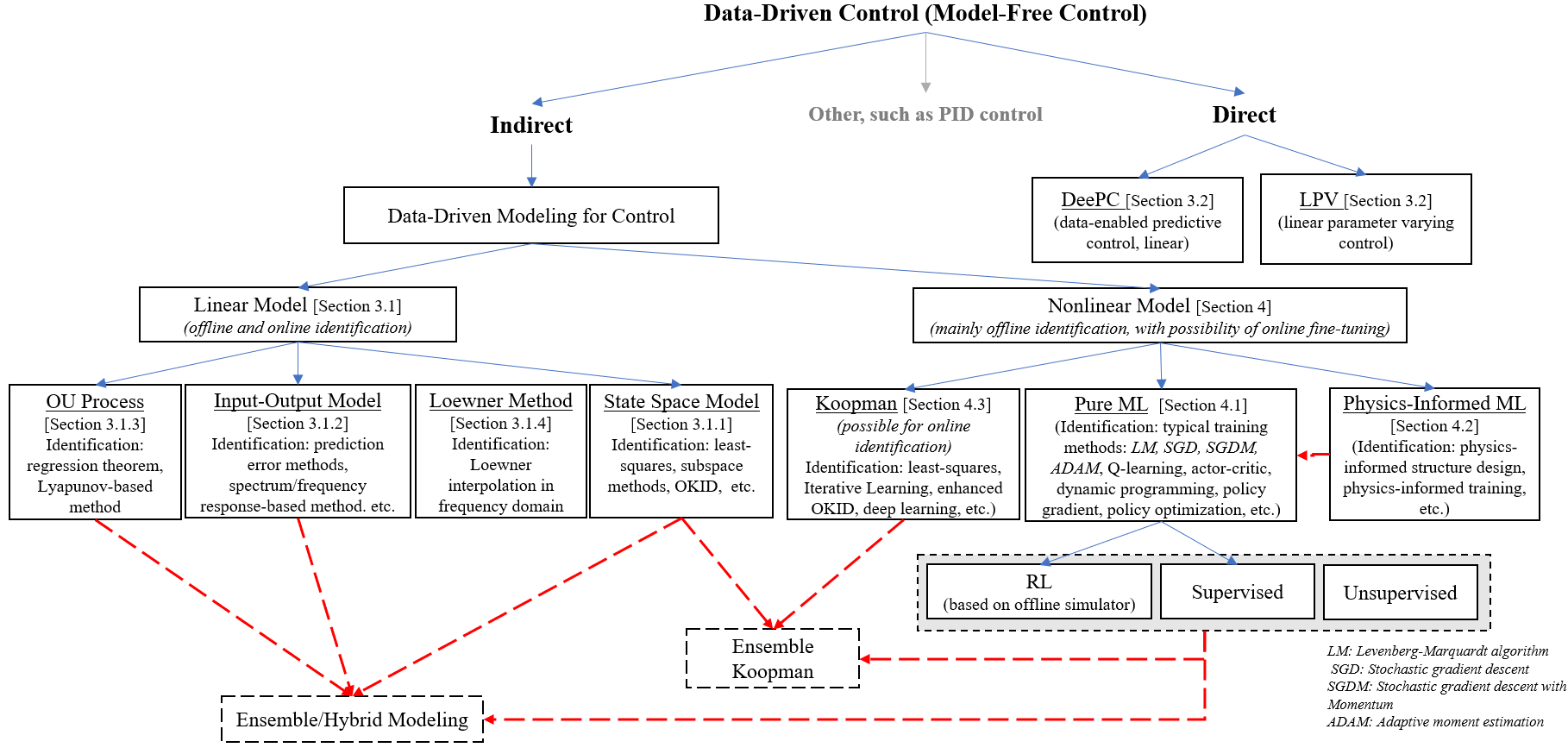
Figure 5: Methodology category for data-driven identification and control.

5.1 Overview of Existing and Potential Power Grid Applications

The data-driven methods are generic and can be tailored for various grid applications. According to the existing work listed in Table 2, we will discuss selective application scenarios of data-driven control. They are oscillation damping control, microgrid control, and aggregated load/EV control.

Oscillation damping control: The first representative application in power grids is the damping control of low-frequency oscillations in either decentralized or centralized manners [42, 15]. As the small signal assumption holds in this application scenario, linear models are generally expressive enough to describe the oscillation modes. Diverse local devices, global network topology and parameters, as well as time-varying operating conditions nowadays make power grid oscillatory dynamics suffer from higher levels of uncertainty, compromising the performance of conventional model-based controllers. Fortunately, such uncertainty can be compensated by data-driven controllers in either a decentralized or centralized fashion. Examples of decentralized adaptive linear data-driven methods are with linear input-output transfer function model [8]), ARMA [42, 148] and DeePC [149, 102]. With the development of wide-area measurement infrastructure, centralized wide-area damping control can be applied to enhance the modeling and thus damping of systemwide interactive oscillation. For example, state space model with subspace identification [51, 49, 85], ARMAX [41], as well as Ornsein-Uhlenbeck process [6, 15, 17] with online parameter estimation are used for damping control with wide-area phasor measurement units. Machine learning such as RL is also used in wide-area damping control to adaptively learn how to address nonlinearity and uncertainty [116]. However, the performance heavily depends on its offline simulator and the adaptation is slow. Considering the simulator fidelity, offline training efficiency and optimality issues, the application purely with RL is not as practical as adaptive linear methods.

Microgrid control: Microgrid control plays a vital role in frequency and voltage regulation/restoration, as well as systemwide power and energy management. Roughly speaking, the dynamics in microgrids span from hundreds of milliseconds to minutes, and the data-driven controller can sample measurements in the range of tens of milliseconds to seconds. Different from traditional power grids, microgrids are characterized by low inertia, coupled states, and wide-frequency dynamics response and are susceptible to high uncertainty and nonlinearity when confronting large disturbances. To address these challenges, nonlinear learning-based methods, such as RL [108, 58, 59, 14], NNs [7, 10, 122] and Koopman-based methods [68, 69] have been employed.

Load/EV control for demand response: Another suitable application scenario of data-driven control in power grids are load and EV control for demand response. The root causes of complicated power consumption dynamics are the combinations of device physical dynamics (e.g., thermal dynamics for thermostatic loads), end-user behavioral dynamics (population dynamics of aggregated load and EVs) as well as the electricity market dynamics. Usually, the end-user information may not be accessed or accurately sensed, introducing uncertainty. The timescale of the aggregation dynamics typically ranges from minutes to hours or even days. The measurements could be sampled by the data-driven controller at the order of minutes from smart meters. From the technical control perspective, a reduced-order state space model is well-suited to efficiently describe the dynamic state evolving of a large population of load or EVs in a linear fashion. This allows for the predictive controller design to realize] full responsiveness to control requests from system operators, while considering the constraints imposed by the normal end use of individual loads/EVs [22]. Online identification on top of the reduced order model is favorable to adapt to the changes associated with weather, financial or social factors that may affect end users. From the commercial operation perspective (e.g., economic dispatch, power tracking quality, grid service provision), nonlinear methods such as RL [61, 113, 21, 150] can directly address the nonlinearity of electricity market dynamics and end-user behaviors. Usually, stable operation over the timescale of hours is the prerequisite to investigate optimal scheduling and operation. Therefore, the application of machine learning is practical in this context, as training efficiency is usually not the primary concern.

5.2 Practicality Overview of Data-Driven Control Methods

The data-driven identification and control can be conducted based on three types of measurement data (ambient, transient, and probing data) [41]. Among them, the ambient data and transient data are suitable for online applications when subject to ambient conditions and large disturbances, respectively. The probing data means actively injecting a probing signal into the system. The signal needs to consistently excite the system to obtain informative datasets, and the probing can deteriorate the electricity quality of power grids.

The data availability, granularity and quantity highly depend on the grid application scenarios and the methods adopted. Use the three selective grid applications discussed in Section 5.1 as examples. They usually adopt different identification and control methods and thus have different data requirements. Linear models are well-suited for oscillation damping control, while nonlinear methods are gaining popularity for microgrid control and demand response. Linear models typically require a relatively small volume of data. For example, in wide-area damping control, accurate identification of linear models can be achieved with online data consisting of a window length of 180-300 seconds of ambient data [15, 41] or 10-second ring-down data [41] sampled at a frequency of 30Hz from wide-area synchrophasor measurements. On the other hand, the nonlinear methods usually need to train a model offline with large volumes of data (e.g., tens of thousands of examples or more) to obtain a deterministic warm-up reference, which then can be fine-tuned online with a small piece of data to adapt to varying uncertainty. Koopman-based methods have the potential to use a small volume of data that are comparable to linear models without the need of warm-up training, thus having the potential to realize faster and more accurate adaptation for grid nonlinear dynamics provided that the Koopman state space (approximating the Koopman embedding mapping) is properly predetermined.

The quality requirements of data are mainly determined by the preprocessing techniques and the data-driven identification and control methods employed. Even within the same method category, different algorithms for preprocessing, identification, and control may have varying data requirements based on the application scenario. Thus, it is challenging to establish exact requirements that are universally applicable. Data preprocessing can involve proper filtering and interpolation to improve data quality. Stochastic optimal identification (e.g., OU process regression theorem, Kalman filtering) and robust control design (e.g., $H_{\infty}$, LMI) can also be incorporated to reduce the requirements on data quality. Table 3 provides a brief overview of commonly used models and their corresponding data requirements for three selected grid application scenarios.

Table 3

Summary on Dominant Modeling Methods and Data Requirement

for Selective Grid Applications

5.3 Online Identification for Different Categories of Data-Driven Control

Online adaptiveness is a desirable feature in power systems due to the time-varying nonlinearity and complexity they exhibit. By utilizing a small amount of online data, online identification effectively addresses uncertainty and mitigates modeling issues. Online identification can be integrated into all categories of data-driven control methods, though it may be inherently easier in some categories compared to others.

For linear data-driven identification and control. Generally, most of the linear data-driven identification and control methods discussed in Section 3 are more computationally efficient than nonlinear methods, thus they can realize online identification and control by using rolling windows, so long as the identification at each time step can be completed within a time interval specified for the grid application of interest. For example, the rolling window-based online identification has been used to online identify OU process models for wide-area voltage control [6] and dynamic load modeling [95]. In some cases, recursive formulations can further improve the algorithms’ efficiency. For example, the recursive or stochastic subspace methods have been used to online identify state space model for adaptive damping control [83, 82] and electromechanical mode estimation [81]. The recursive least-squares method has been used to online identify linear ARMAX models for adaptive control of a converter in a grid-tied microgrid [148] and of power system stabilizer [42]. The recursive estimations of some matrix quantities [96] have been used to online identify OU process linear models for the estimation of dynamic system state matrix of multi-machine power grids.

For machine learning-based nonlinear identification. The idea of pre-training and online tuning was explored for power system analysis in nineties [54]. In 1999, adaptive neuro-identifier and -controller were proposed in [121] for power system stabilizer in a multi-machine power system. These approaches involved obtaining a pre-trained machine learning model through offline warm-up training, which served as a deterministic baseline for subsequent online tuning. This baseline helped reduce output oscillation [121]. Nonetheless, the reliability of adaptive machine learning-based methods is limited due to the lack of physical interpretability and the biased information from online data. Deserved to be mentioned, such an offline-training online-tuning paradigm aligns with the concept of transferable features and learning in the machine learning community, which aims to transfer the knowledge learned from existing system data to new similar systems through offline training, with fine-tuning of learning machine parameters when new data is available [120]. The development of transfer learning techniques nowadays [151] may provide additional opportunities for researchers in power sectors to borrow up-to-date ideas from machine learning community to realize more time-efficient and reliable adaptive learning for nonlinear data-driven control, in terms of trade-offing present and past data in a rolling and more intelligent fashion.

For Koopman-based methods. To our best knowledge, Koopman-based models provide an opportunity to realize online nonlinear identification. They are well suited for online identification by nature due to the linearity after Koopman embedding mapping. They are particularly favorable when obtaining a “warm-up” model is challenging due to limited on-field data volume and runtime requirements. For example, Koopman-based microgrid secondary voltage and frequency control [68, 69] were successfully implemented without warm-up training, even when the microgrid configuration and control parameters were unknown. However, the determination of the Koopman state space still relies on empirical methods. An alternative approach is to pre-learn Koopman generators using physics-informed machine learning and offline data in power grid control. This allows for estimating optimal and physically consistent Koopman operators based on physical states and control inputs. Subsequently, the parameters of the Koopman state space model can be identified online in a linear identification manner.

5.4 Future Trend

Modern power systems have increasingly high uncertainty and nonlinearity due to the increasing penetration of inverter-based resources, leading to more complex system dynamics within wider frequency bands than conventional power grids. As a result, modeling efficacy tends to be more problematic. Conventional machine learning-based methods may not be able to realize satisfactory control performance efficiently and safely due to increasingly high complexity of power grids and the “black-box” nature of machine learning. Emerging data-driven control methods could better address uncertainty and nonlinearity, while being interpretable or having certain physics-informed performance guarantees to enable their applications in real-world power systems. In what follows, we will briefly discuss the trend of each method category.

5.4.1 Linear Data-Driven Identification and Control

Linear data-driven identification and control are still trending in certain power grid applications when the introduced model uncertainty is reasonably bounded (i.e., the small signal assumption roughly holds). A typical example is oscillation damping control as discussed in Section 5.1. However, with the increasingly high penetration of volatile renewables and power electronics devices, the nonlinearity makes the effectiveness of linear models compromised. Nevertheless, adaptive linear control with online identification has the potential to address this issue to some extent by compensating for time-varying model uncertainty owing to the high learning efficiency and fewer data requirements of linear models, while needing further investigation to consolidate in practical applications.

Data-enabled predictive control (DeePC), a direct linear control method, is also emerging in control community and deserves attention for power grid applications. It is an efficient direct data-driven control method based on behavioral systems theory to learn a non-parametric system model that synthesizes the optimality of both identification and control[101]. The direct equivalence between DeePC and subspace predictive control has been demonstrated [152]. Adding quadratic regularization terms with DeePC leads to more robust identification against data noise [153]. Although DeePC is still in the early stage, the linear nature is of potential to combine with online learning to adaptively address time-varying uncertainty and adopt Koopman operator-based structures to address nonlinearity. Also, direct optimal identification and control with a small piece of data subject to disturbances and noises may be further developed.

5.4.2 Machine Learning-Based Methods

It is vital in real-world applications to ensure safe operation after applying any designed controllers. Generally speaking, most of the existing machine learning methods are based on universal approximators but the learning space for parametric training is too broad. Therefore, training of these universal learning machines is often mathematically (sub)optimal for training data while not being reasonable/generalizable for unforeseen cases in real-world applications. This tends to cause over-fitting and compromise the modeling reliability for safety-critical power grids. Among different machine learning-based methods discussed in Section 4, RL-based methods are the most popular nowadays and seem trending as they are where machine learning meets the feedback control. However, the time-consuming training (e.g., tens of thousands of iterations to converge [2]) compromises the fast deployment and adaption to time-varying operating conditions and grid topologies. From the cyberinfrastructure perspective, their practical applications rely on data platforms with sufficient computing resources, data repositories, communication and appropriate technologies to improve training efficiency. From the power grid operation perspective, most of RLs are “black-box” without enough physical interpretability and are not tractable to facilitate the incorporation of physics-inspired information. The safety and scalability of the power grid applications are problematic too.

To further enhance the RL reliability for increasingly complex power grids, safe exploration methods in RL can be considered to bound the parametric learning within a safety region [154]. Another possible way is to add safety constraints at the learned control policy in RL by either incorporating constraints [155] or adding a heuristic safety layer to adjust the control actions [2]. In addition to directly adding the safety constraints/layers in “black-box” RL framework, the power grid modeling and control can be enhanced in a more interpretable framework by incorporating physics-inspired information in RL. For example, the Markov decision processes can be constrained with Bayesian to include physical priors through value or policy functions [67, 27]. Additionally, model predictive control can be combined with RL, whereby the model information can be better incorporated into RL frameworks when applicable. For example, the authors in [156] leverage model predictive control (MPC) and an RL paradigm (dynamic programming), whereby more information can be processed effectively with enhanced reliability, and fast convergence in learning can be achieved. In addition, the standard nonlinear model predictive control (NMPC) scheme can be used as a function approximator in RL, through which the RL can benefit from the rich theory of NMPC with enhanced interpretability on closed-loop performance [66]. Although these methods have yet to be fully investigated for power system applications, they are potential to data-driven model reliability and thus help augment grid operation safety. Some other technical trends in RL research community for more reliable learning also worth attention, including but not limited to the interpretable RL for enhanced consistency in safety-critical applications [157], transfer RL[158] and meta RL for improving adaptiveness to new situations [159], federated RL to preserve data-privacy [160], Bayesian RL to incorporate uncertainty and prior knowledge in learning [67], inverse RL to extract proper reward functions that the RL agents seek to maximize [161], integral RL for continuous-time dynamics modeling [162], etc.

Supervised learning-based surrogate models may also be designed for modern power grid control systems with physical information incorporated by unsupervised learning. The optimization objectives in such a learning paradigm are [163]: (a) to minimize the training error of supervised learning, and meanwhile (b) to minimize a certain physics-informed error of unsupervised learning to regularize the supervised learning in (a). By incorporating regularization through unsupervised learning rather than directly adding regularization terms in objective functions, the generalization of learning machines can be improved due to the powerful unsupervised learning capacity and physics-informed shrink of parameter searching space. Similar ideas can be found in semi-supervised learning for power flow analysis in [164], where auto-encoders (i.e., a decoder + an encoder) are used to incorporate supervised and unsupervised learning. The encoder is where one can include physical knowledge of power grids such as the power mismatches [165], system topology information, etc [164]. Besides, not only the constraints of systemwide power flow but also that of local DERs can be included during the model design and training phases such that more interpretable machine learning-based methods can be realized.

5.4.3 Koopman-Based Methods and Others

The above physics-inspired modeling techniques are often trained with adequate offline datasets while rarely used for online modeling and real-time control. Thus, they may lack fast adaptiveness to time-varying operating conditions of modern power grids. In addition, the identification using the closed-loop control data is also challenging due to the time-varying uncertainty from control input channels. In view of the authors, a dynamics-interpretable Koopman-inspired structure (e.g., Koopman operators and their variants such as EDMD and SINDy) with the help of emerging physics-informed techniques are promising for online learning regarding adaptiveness and scalability. Specifically, the Koopman observables $\Phi(\bm{x},\bm{u})$ in (19) or the basis library $\bm{\Theta}$ in (21) define the Koopman-based model structure, which is the prerequisite for achieving certain physics interpretability on system dynamics and thus improving data-driven model efficacy and transparency for data-driven dynamical control.

Although promising, Koopman-based methods are still in the early stages of development. One of the main challenges limiting the applications of Koopman-based methods into power grids is the difficulty in determining the Koopman basis (i.e., Koopman observables or eigenfunctions) that formulates a proper Koopman state space structure. By and large, the Koopman basis is empirically determined based on power grid domain knowledge or learned directly from data with either universal training or self-dictation based on the dynamic relationship of the Koopman-based space and the original space [137, 138, 139, 140, 141]. For example, in high-inertia power grids dominated by multiple machines, the system dynamics are mainly driven by electromechanics, and the candidates of Koopman basis functions can be relatively straightforward (the combination of the trigonometric functions [11, 135]) by considering the differential equations of the electromechanical physical models and the network power flow. Although no guarantee for optimal design, the dominant dynamical characteristics can be well-captured. However, in future power grids with greater modernization, the determination of Koopman state space merely based on observation may not always work due to complex dynamics resulting from low inertia, a large number of diverse distributed energy resources, varying operating conditions as well as fast-evolving network topologies. The advancements of machine learning techniques now and future will offer tremendous opportunities to learn optimal Koopman embedding mapping. For example, a potential solution is to apply Koopman-based modeling in the RL frameworks, in which the Koopman-based methods can help RL enhance environment/value/policy function modeling and the RL framework in turn can help Koopman-based methods explore the problem inherent structure by pursuing Bellman optimality [57]. Besides, physics-inspired domain information in power grids has yet to be incorporated in the deep learning-based Koopman basis discovery while deserving more attention.

Given appropriate Koopman structures, the development of Koopman-based online estimation and control are also trending because of their structural advantages inherited from linear systems. First, as Koopman operator-based space is linear, mature linear identification techniques are applicable to enhance identification, which could be used for power grid applications in the future. For example, the linear matrix inequality (LMI) can be used to relax the minimization of the loss function with regularization terms (i.e., (17) or (18c)) to convex problems [166, 167], which can help realize modular, optimal and fast identification. Besides, the mechanism with recursive measurement data may be designed to improve Koopman-based identification efficiency aiming at faster adaption to time-varying uncertainty and nonlinearity. Second, online ensemble learning to combine individual models is another way to further improve identification. For example, a “soft switching” mechanism [117] can be employed to weigh linear and nonlinear models [7], and an online iterative ensemble structure[68] can be used to combine small-signal physical models and large-signal models. Nonetheless, the stability and optimality of online ensemble control remain to be investigated. Third, the Koopman-enabled linear structure provides opportunities for the applications of distributed and cooperative MPC [168, 169, 170], which are mature control techniques with well-characterized stability and robustness properties. This shed light on potential practical solutions to scalable integration of distributed energy resources into modern power grids.

5.4.4 Data Sources

To the best of our knowledge, almost all the existing RL-based control are based on power system simulators. The supervised learning-based modeling and Koopman-based modeling for control are based on simulation data, historical experimental offline data or online data. Real-time simulation is an emerging trend that enables the development of high-fidelity simulators for complex modern power systems, offering the potential for future implementation of “digital twins” for online monitoring and control. The digital twin is an up-to-date representation of an actual current asset in operation that includes the asset’s condition and relevant historical data [171]. The real-time simulator and ultimately the digital twin can be used as the simulator for RL and the full-state data generator for supervised learning. However, it’s important to note that even with high-fidelity simulators or experimental data, there may exist a small gap between these representations and the real-world systems, leading to uncertainty propagation and thus compromising control performance. To mitigate this, some countermeasures may be taken such as robust (adversarial) RL methods in simulator-based policy training [2, 172, 173], and data augmentation techniques, such as adversarial NNs [174], can generate sufficient training data that includes necessary information for robust supervised learning-based modeling for control.

6 Conclusion

This paper provides a comprehensive review on emerging data-driven control for the applications in modern power grids. The data-driven control mainly consists of two ingredients — identification and control, which should be conducted jointly in a either sequential or simultaneous manner. To realize real-world applications for safety-critical power grids of high complexity, physics-informed methodology is necessary while it remains to be studied to realize a practical solution that is theoretically sound with performance guarantee. In general, one needs to consider the physical constraints and find elegant ways to incorporate them in identification and control. To this end, combining learning-based methods, physical domain knowledge, and the Koopman-based model structure seems promising as mature linear system control methods with well-characterized stability and robustness can be readily applied to the linear Koopman-based model. Besides, various machine learning methods including supervised, unsupervised learning and RL may be used jointly in exploring and exploiting model structure and parameters with proper physics-informed learning objectives and constraints defined by users.

References

- [1] P. D. Lund, J. Byrne, R. Haas, D. Flynn, Advances in Energy Systems: The Large-scale Renewable Energy Integration Challenge, 1st Edition, John Wiley & Sons, google-Books-ID: cA6GDwAAQBAJ.
- [2] X. Chen, G. Qu, Y. Tang, S. Low, N. Li, Reinforcement learning for selective key applications in power systems: Recent advances and future challenges, IEEE Transactions on Smart Grid 13 (4) (2022) 2935–2958. doi:10.1109/TSG.2022.3154718.
- [3] D. E. Olivares, A. Mehrizi-Sani, A. H. Etemadi, C. A. Cañizares, R. Iravani, M. Kazerani, A. H. Hajimiragha, O. Gomis-Bellmunt, M. Saeedifard, R. Palma-Behnke, G. A. Jiménez-Estévez, N. D. Hatziargyriou, Trends in microgrid control, IEEE Transactions on Smart Grid 5 (4) (2014) 1905–1919. doi:10.1109/TSG.2013.2295514.
- [4] A. Bidram, A. Davoudi, Hierarchical structure of microgrids control system, IEEE Transactions on Smart Grid 3 (4) (2012) 1963–1976. doi:10.1109/TSG.2012.2197425.
- [5] J. Wang, H. Padullaparti, S. Veda, I. Mendoza, S. Tiwari, M. Baggu, Performance evaluation of data-enhanced hierarchical control for grid operations, in: 2020 IEEE Power & Energy Society General Meeting (PESGM), 2020, pp. 1–5. doi:10.1109/PESGM41954.2020.9281456.
- [6] G. Pierrou, X. Wang, An online network model-free wide-area voltage control method using pmus, IEEE Transactions on Power Systems 36 (5) (2021) 4672–4682. doi:10.1109/TPWRS.2021.3058642.
- [7] Z. Ma, Z. Wang, Y. Guo, Y. Yuan, H. Chen, Nonlinear multiple models adaptive secondary voltage control of microgrids, IEEE Transactions on Smart Grid 12 (1) (2021) 227–238. doi:10.1109/TSG.2020.3023307.
- [8] D. J. Ryan, R. Razzaghi, H. D. Torresan, A. Karimi, B. Bahrani, Grid-supporting battery energy storage systems in islanded microgrids: A data-driven control approach, IEEE Transactions on Sustainable Energy 12 (2) (2021) 834–846. doi:10.1109/TSTE.2020.3022362.
- [9] M. Zholbaryssov, A. D. Domínguez-García, Safe data-driven secondary control of distributed energy resources, IEEE Transactions on Power Systems 36 (6) (2021) 5933–5943. doi:10.1109/TPWRS.2021.3084440.
- [10] D.-D. Zheng, S. S. Madani, A. Karimi, Data-driven distributed online learning control for islanded microgrids, IEEE Journal on Emerging and Selected Topics in Circuits and Systems 12 (1) (2022) 194–204. doi:10.1109/JETCAS.2022.3152938.
- [11] M. Korda, Y. Susuki, I. Mezić, Power grid transient stabilization using koopman model predictive control, IFAC-PapersOnLine 51 (28) (2018) 297–302. doi:https://doi.org/10.1016/j.ifacol.2018.11.718.
- [12] Y. Asadi, M. M. Farsangi, A. M. Amani, E. Bijami, H. H. Alhelou, Data-driven automatic generation control of interconnected power grids subject to deception attacks, IEEE Internet of Things Journal (2022) 1–1doi:10.1109/JIOT.2022.3182978.
- [13] S. S. Madani, C. Kammer, A. Karimi, Data-driven distributed combined primary and secondary control in microgrids, IEEE Transactions on Control Systems Technology 29 (3) (2021) 1340–1347. doi:10.1109/TCST.2019.2958285.
- [14] P. Chen, S. Liu, B. Chen, L. Yu, Multi-agent reinforcement learning for decentralized resilient secondary control of energy storage systems against dos attacks, IEEE Transactions on Smart Grid 13 (3) (2022) 1739–1750. doi:10.1109/TSG.2022.3142087.
- [15] I. Zenelis, X. Wang, I. Kamwa, Online pmu-based wide-area damping control for multiple inter-area modes, IEEE Transactions on Smart Grid 11 (6) (2020) 5451–5461. doi:10.1109/TSG.2020.3001607.
- [16] I. Zenelis, X. Wang, Wide-area damping control for interarea oscillations in power grids based on pmu measurements, IEEE Control Systems Letters 2 (4) (2018) 719–724. doi:10.1109/LCSYS.2018.2847758.
- [17] J. Guo, I. Zenelis, X. Wang, B.-T. Ooi, Wams-based model-free wide-area damping control by voltage source converters, IEEE Transactions on Power Systems 36 (2) (2021) 1317–1327. doi:10.1109/TPWRS.2020.3012917.
- [18] Q. Zhou, M. Shahidehpour, A. Alabdulwahab, A. Abusorrah, L. Che, X. Liu, Cross-layer distributed control strategy for cyber resilient microgrids, IEEE Transactions on Smart Grid 12 (5) (2021) 3705–3717. doi:10.1109/TSG.2021.3069331.
- [19] W. Liu, J. Sun, G. Wang, F. Bullo, J. Chen, Data-driven resilient predictive control under denial-of-service, arXiv preprint arXiv:2110.12766.
- [20] J. R. Vázquez-Canteli, Z. Nagy, Reinforcement learning for demand response: A review of algorithms and modeling techniques, Applied energy 235 (2019) 1072–1089.
- [21] M. Liu, S. Peeters, D. S. Callaway, B. J. Claessens, Trajectory tracking with an aggregation of domestic hot water heaters: Combining model-based and model-free control in a commercial deployment, IEEE Transactions on Smart Grid 10 (5) (2019) 5686–5695. doi:10.1109/TSG.2018.2890275.
- [22] J. L. Mathieu, D. S. Callaway, State estimation and control of heterogeneous thermostatically controlled loads for load following, in: 2012 45th Hawaii International Conference on System Sciences, 2012, pp. 2002–2011. doi:10.1109/HICSS.2012.545.
- [23] X. Gong, E. Castillo-Guerra, J. L. Cardenas-Barrera, B. Cao, S. A. Saleh, L. Chang, Robust hierarchical control mechanism for aggregated thermostatically controlled loads, IEEE Transactions on Smart Grid 12 (1) (2021) 453–467. doi:10.1109/TSG.2020.3009989.
- [24] Z. Hou, R. Chi, H. Gao, An overview of dynamic-linearization-based data-driven control and applications, IEEE Transactions on Industrial Electronics 64 (5) (2016) 4076–4090.
- [25] Z.-S. Hou, Z. Wang, From model-based control to data-driven control: Survey, classification and perspective, Information Sciences 235 (2013) 3–35.
- [26] L. Hewing, K. P. Wabersich, M. Menner, M. N. Zeilinger, Learning-based model predictive control: Toward safe learning in control, Annual Review of Control, Robotics, and Autonomous Systems 3 (2020) 269–296.
- [27] L. Brunke, M. Greeff, A. W. Hall, Z. Yuan, S. Zhou, J. Panerati, A. P. Schoellig, Safe learning in robotics: From learning-based control to safe reinforcement learning, Annual Review of Control, Robotics, and Autonomous Systems 5 (2022) 411–444.
- [28] Z. Zhang, D. Zhang, R. C. Qiu, Deep reinforcement learning for power system applications: An overview, CSEE Journal of Power and Energy Systems 6 (1) (2020) 213–225. doi:10.17775/CSEEJPES.2019.00920.
- [29] B. She, F. Li, H. Cui, J. Zhang, R. Bo, Fusion of microgrid control with model-free reinforcement learning: Review and vision, IEEE Transactions on Smart Grid (2022) 1–1doi:10.1109/TSG.2022.3222323.
- [30] G. S. Misyris, A. Venzke, S. Chatzivasileiadis, Physics-informed neural networks for power systems, in: 2020 IEEE Power & Energy Society General Meeting (PESGM), 2020, pp. 1–5. doi:10.1109/PESGM41954.2020.9282004.
- [31] K. Zarkogianni, K. S. Nikita, Personal health systems for diabetes management, early diagnosis and prevention, in: Consumer-Driven Technologies in Healthcare: Breakthroughs in Research and Practice, IGI Global, 2019, pp. 191–218.
- [32] B. Egardt, Stability of adaptive controllers, Springer, 1979.
- [33] J. Smith, F. Fatehi, C. Woods, J. Hauer, D. Trudnowski, Transfer function identification in power system applications, IEEE Transactions on Power Systems 8 (3) (1993) 1282–1290. doi:10.1109/59.260866.
- [34] I. Kamwa, R. Grondin, E. Dickinson, S. Fortin, A minimal realization approach to reduced-order modelling and modal analysis for power system response signals, IEEE Transactions on Power Systems 8 (3) (1993) 1020–1029.
- [35] J. Sanchez-Gasca, D. Trudnowski, E. Barocio, J. Hauer, J. W. Pierre, C. Canizares, H. Huang, T. Rauhala, J. H. Chow, I. Kamwa, et al., Identification of electromechanical modes in power systems, in: IEEE Task Force Report, Special Publication TP462, IEEE, 2012.
- [36] I. Kamwa, L. Gerin-Lajoie, State-space system identification-toward mimo models for modal analysis and optimization of bulk power systems, IEEE Transactions on Power Systems 15 (1) (2000) 326–335.
- [37] I. Kamwa, G. Trudel, L. Gerin-Lajoie, Low-order black-box models for control system design in large power systems, in: Proceedings of Power Industry Computer Applications Conference, 1995, pp. 190–198. doi:10.1109/PICA.1995.515183.
- [38] J. Zhang, C. Lu, Y. Han, Mimo identification of power system with low level probing tests: Applicability comparison of subspace methods, IEEE Transactions on Power Systems 28 (3) (2013) 2907–2917. doi:10.1109/TPWRS.2013.2239316.
- [39] G. Gurrala, Loewner matrix approach for modelling fdnes of power systems, Electric Power Systems Research 125 (2015) 116–123.
- [40] C. Rergis, I. Kamwa, R. Khazaka, A. Messina, A loewner interpolation method for power system identification and order reduction, IEEE Transactions on Power Systems 34 (3) (2018) 1834–1844.
- [41] H. Liu, L. Zhu, Z. Pan, F. Bai, Y. Liu, Y. Liu, M. Patel, E. Farantatos, N. Bhatt, Armax-based transfer function model identification using wide-area measurement for adaptive and coordinated damping control, IEEE Transactions on Smart Grid 8 (3) (2017) 1105–1115. doi:10.1109/TSG.2015.2470648.
- [42] G. Ramakrishna, O. Malik, Adaptive pss using a simple on-line identifier and linear pole-shift controller, Electric Power Systems Research 80 (4) (2010) 406–416.
- [43] F. A. Zelaya A., J. H. Chow, M. Paternina, A. Zamora, Power system linear model selective identification by exploiting the loewner interpolation method, in: 2020 IEEE Power & Energy Society General Meeting (PESGM), 2020, pp. 1–5. doi:10.1109/PESGM41954.2020.9282088.
- [44] O. F. Ruiz-Martinez, J. C. Mayo-Maldonado, G. Escobar, B. A. Frias-Araya, J. E. Valdez-Resendiz, J. C. Rosas-Caro, P. Rapisarda, Data-driven control of lvdc network converters: Active load stabilization, IEEE Transactions on Smart Grid 11 (3) (2020) 2182–2194. doi:10.1109/TSG.2019.2949259.
- [45] Y. Zhao, L. Zhu, H. Xiao, Y. Liu, E. Farantatos, M. Patel, A. Darvishi, B. Fardanesh, An adaptive wide-area damping controller via facts for the new york state grid using a measurement-driven model, in: 2019 IEEE Power & Energy Society General Meeting (PESGM), 2019, pp. 1–5. doi:10.1109/PESGM40551.2019.8973540.
- [46] A. Barkley, E. Santi, Improved online identification of a dc–dc converter and its control loop gain using cross-correlation methods, IEEE Transactions on Power Electronics 24 (8) (2009) 2021–2031. doi:10.1109/TPEL.2009.2020588.
- [47] H. Zhang, J. Zhou, Q. Sun, J. M. Guerrero, D. Ma, Data-driven control for interlinked ac/dc microgrids via model-free adaptive control and dual-droop control, IEEE Transactions on Smart Grid 8 (2) (2015) 557–571.
- [48] D. Yang, B. Wang, G. Cai, J. Ma, J. Tian, Z. Chen, L. Wang, Inertia-adaptive model predictive control-based load frequency control for interconnected power systems with wind power, IET Generation, Transmission & Distribution 14 (22) (2020) 5029–5036.
- [49] R. Eriksson, L. Söder, Wide-area measurement system-based subspace identification for obtaining linear models to centrally coordinate controllable devices, IEEE Transactions on Power Delivery 26 (2) (2011) 988–997. doi:10.1109/TPWRD.2010.2094628.
- [50] R. Eriksson, L. Soder, Wide-area measurement system control to coordinate hvdc links in large scale power systems, in: 2011 16th International Conference on Intelligent System Applications to Power Systems, 2011, pp. 1–5. doi:10.1109/ISAP.2011.6082169.
- [51] J. D. Nieto, J. M. Mauricio, Power system optimal wide area control based on identified models, in: 2015 IEEE Eindhoven PowerTech, 2015, pp. 1–6. doi:10.1109/PTC.2015.7232742.
- [52] Y. Zhang, L. Xie, Q. Ding, Interactive control of coupled microgrids for guaranteed system-wide small signal stability, IEEE Transactions on Smart Grid 7 (2) (2016) 1088–1096. doi:10.1109/TSG.2015.2495233.
- [53] H. Mori, Y. Tamaru, S. Tsuzuki, An artificial neural-net based technique for power system dynamic stability with the kohonen model, IEEE Transactions on power systems 7 (2) (1992) 856–864.
- [54] I. Kamwa, R. Grondin, V. Sood, C. Gagnon, V. T. Nguyen, J. Mereb, Recurrent neural networks for phasor detection and adaptive identification in power system control and protection, IEEE Transactions on Instrumentation and Measurement 45 (2) (1996) 657–664. doi:10.1109/19.492805.
- [55] B.-Y. Ku, R. J. Thomas, C.-Y. Chiou, C.-J. Lin, Power system dynamic load modeling using artificial neural networks, IEEE Transactions on power systems 9 (4) (1994) 1868–1874.
- [56] M. Bostanci, J. Koplowitz, C. Taylor, Identification of power system load dynamics using artificial neural networks, IEEE Transactions on Power Systems 12 (4) (1997) 1468–1473.
- [57] S. Haykin, Neural networks and learning machines, 3rd Edition, PHI Learning.
- [58] P. Kou, D. Liang, C. Wang, Z. Wu, L. Gao, Safe deep reinforcement learning-based constrained optimal control scheme for active distribution networks, Applied energy 264 (2020) 114772.
- [59] M. H. Khooban, M. Gheisarnejad, A novel deep reinforcement learning controller based type-ii fuzzy system: Frequency regulation in microgrids, IEEE Transactions on Emerging Topics in Computational Intelligence 5 (4) (2021) 689–699. doi:10.1109/TETCI.2020.2964886.
- [60] Z. Wan, H. Li, H. He, D. Prokhorov, Model-free real-time ev charging scheduling based on deep reinforcement learning, IEEE Transactions on Smart Grid 10 (5) (2019) 5246–5257. doi:10.1109/TSG.2018.2879572.
- [61] V.-H. Bui, A. Hussain, H.-M. Kim, Double deep -learning-based distributed operation of battery energy storage system considering uncertainties, IEEE Transactions on Smart Grid 11 (1) (2020) 457–469. doi:10.1109/TSG.2019.2924025.
- [62] Q. Huang, R. Huang, W. Hao, J. Tan, R. Fan, Z. Huang, Adaptive power system emergency control using deep reinforcement learning, IEEE Transactions on Smart Grid 11 (2) (2020) 1171–1182. doi:10.1109/TSG.2019.2933191.
- [63] Z. Xu, Y. Zan, C. Xu, J. Li, D. Shi, Z. Wang, B. Zhang, J. Duan, Accelerated drl agent for autonomous voltage control using asynchronous advantage actor-critic, in: 2020 IEEE Power & Energy Society General Meeting (PESGM), 2020, pp. 1–5. doi:10.1109/PESGM41954.2020.9281768.
- [64] R. Huang, Y. Chen, T. Yin, X. Li, A. Li, J. Tan, W. Yu, Y. Liu, Q. Huang, Accelerated derivative-free deep reinforcement learning for large-scale grid emergency voltage control, IEEE Transactions on Power Systems 37 (1) (2022) 14–25. doi:10.1109/TPWRS.2021.3095179.
- [65] B. Huang, J. Wang, Applications of physics-informed neural networks in power systems - a review, IEEE Transactions on Power Systems 38 (1) (2023) 572–588. doi:10.1109/TPWRS.2022.3162473.
- [66] S. Gros, M. Zanon, Data-driven economic nmpc using reinforcement learning, IEEE Transactions on Automatic Control 65 (2) (2020) 636–648. doi:10.1109/TAC.2019.2913768.
- [67] M. Ghavamzadeh, S. Mannor, J. Pineau, A. Tamar, et al., Bayesian reinforcement learning: A survey, Foundations and Trends® in Machine Learning 8 (5-6) (2015) 359–483.
- [68] X. Gong, X. Wang, G. Joos, An online data-driven method for microgrid secondary voltage and frequency control with ensemble koopman modeling, IEEE Transactions on Smart Grid (2022) 1–1doi:10.1109/TSG.2022.3190237.
- [69] X. Gong, X. Wang, A novel koopman-inspired method for the secondary control of microgrids with grid-forming and grid-following sources, Applied Energy 333 (2023) 120631.
- [70] F. Dorfler, J. Coulson, I. Markovsky, Bridging direct & indirect data-driven control formulations via regularizations and relaxations, IEEE Transactions on Automatic Control (2022) 1–1doi:10.1109/TAC.2022.3148374.
- [71] H. Ghasemi, C. Canizares, A. Moshref, Oscillatory stability limit prediction using stochastic subspace identification, IEEE Transactions on Power Systems 21 (2) (2006) 736–745. doi:10.1109/TPWRS.2006.873100.
- [72] I. W. Jamaludin, N. A. Wahab, N. S. Khalid, S. Sahlan, Z. Ibrahim, M. F. Rahmat, N4sid and moesp subspace identification methods, in: 2013 IEEE 9th International Colloquium on Signal Processing and its Applications, 2013, pp. 140–145. doi:10.1109/CSPA.2013.6530030.
- [73] M. Mansouri, D. Westwick, A. M. Knight, A n4sid-based strategy to estimate the parameters of disturbances in power systems, in: 2018 IEEE PES Innovative Smart Grid Technologies Conference Europe (ISGT-Europe), 2018, pp. 1–6. doi:10.1109/ISGTEurope.2018.8571689.
- [74] R. Vikhram Yohanandhan, L. Srinivasan, Decentralised wide-area fractional order damping controller for a large-scale power system, IET Generation, Transmission & Distribution 10 (5) (2016) 1164–1178.
- [75] L. Zhu, H. Liu, Y. Ma, Y. Liu, E. Farantatos, M. Patel, S. McGuinness, Adaptive and coordinated oscillation damping control using measurement-driven approach, in: 2016 Power Systems Computation Conference (PSCC), 2016, pp. 1–7. doi:10.1109/PSCC.2016.7540932.
- [76] L. Dosiek, N. Zhou, J. W. Pierre, Z. Huang, D. J. Trudnowski, Mode shape estimation algorithms under ambient conditions: A comparative review, IEEE Transactions on Power Systems 28 (2) (2012) 779–787.
- [77] H. Ye, Y. Liu, Online recursive closed-loop state space model identification for damping control, in: 2010 Asia-Pacific Power and Energy Engineering Conference, 2010, pp. 1–4. doi:10.1109/APPEEC.2010.5448424.
- [78] A. Alenany, D. Westwick, H. Shang, A modified observer/kalman filter identification (OKID) algorithm employing output residuals 7 (2) 636–643. doi:10.1007/s40435-018-00502-9.
- [79] T. Katayama, et al., Subspace methods for system identification, Vol. 1, Springer, 2005.
- [80] S. J. Qin, An overview of subspace identification, Computers & Chemical Engineering 30 (10) (2006) 1502–1513. doi:https://doi.org/10.1016/j.compchemeng.2006.05.045.
- [81] S. N. Sarmadi, V. Venkatasubramanian, Electromechanical mode estimation using recursive adaptive stochastic subspace identification, IEEE Transactions on Power Systems 29 (1) (2013) 349–358.
- [82] P. Zhang, D. Yang, K. W. Chan, G. Cai, Adaptive wide-area damping control scheme with stochastic subspace identification and signal time delay compensation, IET generation, transmission & distribution 6 (9) (2012) 844–852.
- [83] B. Wu, O. P. Malik, Multivariable adaptive control of synchronous machines in a multimachine power system, IEEE Transactions on Power Systems 21 (4) (2006) 1772–1781.
- [84] R. Eriksson, L. Söder, Wide-area measurement system-based subspace identification for obtaining linear models to centrally coordinate controllable devices, IEEE Transactions on Power Delivery 26 (2) (2011) 988–997. doi:10.1109/TPWRD.2010.2094628.
- [85] Y. Hua, L. Yutian, Design of model predictive controllers for adaptive damping of inter-area oscillations, International Journal of Electrical Power & Energy Systems 45 (1) (2013) 509–518.
- [86] L. Ljung, System Identification: Theory for the User, Prentice Hall information and system sciences series, Prentice Hall PTR, 1999.
- [87] Y. Zhao, B. Huang, H. Su, J. Chu, Prediction error method for identification of lpv models, Journal of process control 22 (1) (2012) 180–193.
- [88] L. Ljung, Prediction error estimation methods, Circuits, Systems and Signal Processing 21 (2002) 11–21.
- [89] A. Karimi, C. Kammer, A data-driven approach to robust control of multivariable systems by convex optimization, Automatica 85 (2017) 227–233. doi:https://doi.org/10.1016/j.automatica.2017.07.063.
- [90] W. Yao, L. Jiang, J. Wen, Q. Wu, S. Cheng, Wide-area damping controller for power system interarea oscillations: A networked predictive control approach, IEEE Transactions on Control Systems Technology 23 (1) (2014) 27–36.
- [91] Z. Hou, S. Jin, Data-driven model-free adaptive control for a class of mimo nonlinear discrete-time systems, IEEE Transactions on Neural Networks 22 (12) (2011) 2173–2188. doi:10.1109/TNN.2011.2176141.
- [92] C. Paleologu, J. Benesty, S. Ciochina, A robust variable forgetting factor recursive least-squares algorithm for system identification, IEEE Signal Processing Letters 15 (2008) 597–600. doi:10.1109/LSP.2008.2001559.
- [93] S. Rogers, Adaptive filter theory, Control Engineering Practice 4 (11) (1996) 1629–1630.
- [94] C. Lu, Y. Zhao, K. Men, L. Tu, Y. Han, Wide-area power system stabiliser based on model-free adaptive control, IET Control Theory & Applications 9 (13) (2015) 1996–2007.
- [95] G. Pierrou, X. Wang, Online pmu-based method for estimating dynamic load parameters in ambient conditions, in: 2020 IEEE Power & Energy Society General Meeting (PESGM), 2020, pp. 1–5. doi:10.1109/PESGM41954.2020.9281825.
- [96] H. Sheng, X. Wang, Online measurement-based estimation of dynamic system state matrix in ambient conditions, IEEE Transactions on Smart Grid 11 (1) (2020) 95–105. doi:10.1109/TSG.2019.2917672.
- [97] M. T. Kassis, M. Kabir, Y. Q. Xiao, R. Khazaka, Passive reduced order macromodeling based on loewner matrix interpolation, IEEE Transactions on Microwave Theory and Techniques 64 (8) (2016) 2423–2432.
- [98] M. Kabir, R. Khazaka, Macromodeling of distributed networks from frequency-domain data using the loewner matrix approach, IEEE Transactions on Microwave Theory and Techniques 60 (12) (2012) 3927–3938.
- [99] D. Rimorov, C. M. Rergis, I. Kamwa, A. Moeini, J. Huang, A. Darvishi, B. Fardanesh, Calculating impulse and frequency response of large power system models for realization identification, IEEE Transactions on Power Systems 35 (5) (2020) 3825–3834. doi:10.1109/TPWRS.2020.2981830.
- [100] L. Huang, J. Zhen, J. Lygeros, F. Dörfler, Quadratic regularization of data-enabled predictive control: Theory and application to power converter experiments, IFAC-PapersOnLine 54 (7) (2021) 192–197. doi:https://doi.org/10.1016/j.ifacol.2021.08.357.
- [101] J. Coulson, J. Lygeros, F. Dörfler, Data-enabled predictive control: In the shallows of the deepc, in: 2019 18th European Control Conference (ECC), 2019, pp. 307–312. doi:10.23919/ECC.2019.8795639.
- [102] L. Huang, J. Coulson, J. Lygeros, F. Dörfler, Decentralized data-enabled predictive control for power system oscillation damping, IEEE Transactions on Control Systems Technology 30 (3) (2022) 1065–1077. doi:10.1109/TCST.2021.3088638.
- [103] Y. Zhao, T. Liu, D. J. Hill, A data-enabled predictive control method for frequency regulation of power systems, in: 2021 IEEE PES Innovative Smart Grid Technologies Europe (ISGT Europe), IEEE, 2021, pp. 01–06.
- [104] Y. Zhao, T. Liu, D. Hill, A multi-agent reinforcement learning based frequency control method with data-enabled predictive control guided policy search, in: 2022 IEEE Power & Energy Society General Meeting (PESGM), IEEE, 2022, pp. 01–05.
- [105] S. S. Madani, A. Karimi, Data-driven lpv controller design for islanded microgrids, IFAC-PapersOnLine 54 (7) (2021) 433–438.
- [106] T. T. Nguyen, F. Trahay, J. Domke, A. Drozd, E. Vatai, J. Liao, M. Wahib, B. Gerofi, Why globally re-shuffle? revisiting data shuffling in large scale deep learning, in: 2022 IEEE International Parallel and Distributed Processing Symposium (IPDPS), IEEE, 2022, pp. 1085–1096.
- [107] S. L. Brunton, J. N. Kutz, Data-driven science and engineering: Machine learning, dynamical systems, and control, Cambridge University Press, 2022.
- [108] A. Younesi, H. Shayeghi, P. Siano, Assessing the use of reinforcement learning for integrated voltage/frequency control in ac microgrids, Energies 13 (5) (2020) 1250.
- [109] C. Chen, M. Cui, F. Li, S. Yin, X. Wang, Model-free emergency frequency control based on reinforcement learning, IEEE Transactions on Industrial Informatics 17 (4) (2021) 2336–2346. doi:10.1109/TII.2020.3001095.
- [110] L. Yin, C. Zhang, Y. Wang, F. Gao, J. Yu, L. Cheng, Emotional deep learning programming controller for automatic voltage control of power systems, IEEE Access 9 (2021) 31880–31891. doi:10.1109/ACCESS.2021.3060620.
- [111] F. L. D. Silva, C. E. H. Nishida, D. M. Roijers, A. H. R. Costa, Coordination of electric vehicle charging through multiagent reinforcement learning, IEEE Transactions on Smart Grid 11 (3) (2020) 2347–2356. doi:10.1109/TSG.2019.2952331.
- [112] R. Hao, T. Lu, Q. Ai, H. He, Distributed online dispatch for microgrids using hierarchical reinforcement learning embedded with operation knowledge, IEEE Transactions on Power Systems (2021) 1–1doi:10.1109/TPWRS.2021.3092220.
- [113] H. Li, Z. Wan, H. He, Constrained ev charging scheduling based on safe deep reinforcement learning, IEEE Transactions on Smart Grid 11 (3) (2020) 2427–2439. doi:10.1109/TSG.2019.2955437.
- [114] V. P. Singh, N. Kishor, P. Samuel, Distributed multi-agent system-based load frequency control for multi-area power system in smart grid, IEEE Transactions on Industrial Electronics 64 (6) (2017) 5151–5160. doi:10.1109/TIE.2017.2668983.
- [115] Z. Yan, Y. Xu, A multi-agent deep reinforcement learning method for cooperative load frequency control of a multi-area power system, IEEE Transactions on Power Systems 35 (6) (2020) 4599–4608. doi:10.1109/TPWRS.2020.2999890.
- [116] R. Yousefian, S. Kamalasadan, Energy function inspired value priority based global wide-area control of power grid, IEEE Transactions on Smart Grid 9 (2) (2018) 552–563. doi:10.1109/TSG.2016.2555909.
- [117] Y. Zhang, T. Chai, H. Wang, J. Fu, L. Zhang, Y. Wang, An adaptive generalized predictive control method for nonlinear systems based on anfis and multiple models, IEEE Transactions on Fuzzy Systems 18 (6) (2010) 1070–1082. doi:10.1109/TFUZZ.2010.2062524.
- [118] S. Kazemlou, S. Mehraeen, Decentralized discrete-time adaptive neural network control of interconnected dc distribution system, IEEE Transactions on Smart Grid 5 (5) (2014) 2496–2507.
- [119] G. Shi, X. Shi, M. O’Connell, R. Yu, K. Azizzadenesheli, A. Anandkumar, Y. Yue, S.-J. Chung, Neural lander: Stable drone landing control using learned dynamics, in: 2019 International Conference on Robotics and Automation (ICRA), 2019, pp. 9784–9790. doi:10.1109/ICRA.2019.8794351.
- [120] J. Yosinski, J. Clune, Y. Bengio, H. Lipson, How transferable are features in deep neural networks?, Advances in neural information processing systems 27.
- [121] P. Shamsollahi, O. P. Malik, Application of neural adaptive power system stabilizer in a multi-machine power system, IEEE Transactions on Energy Conversion 14 (3) (1999) 731–736.
- [122] W. Dong, S. Li, X. Fu, Artificial neural network control of a standalone dc microgrid, in: 2018 Clemson University Power Systems Conference (PSC), IEEE, 2018, pp. 1–5.
- [123] P. Gupta, A. Pal, V. Vittal, Coordinated wide-area damping control using deep neural networks and reinforcement learning, IEEE Transactions on Power Systems 37 (1) (2022) 365–376. doi:10.1109/TPWRS.2021.3091940.
- [124] J. Stiasny, G. S. Misyris, S. Chatzivasileiadis, Physics-informed neural networks for non-linear system identification for power system dynamics, in: 2021 IEEE Madrid PowerTech, 2021, pp. 1–6. doi:10.1109/PowerTech46648.2021.9495063.
- [125] G. S. Misyris, J. Stiasny, S. Chatzivasileiadis, Capturing power system dynamics by physics-informed neural networks and optimization, in: 2021 60th IEEE Conference on Decision and Control (CDC), IEEE, 2021, pp. 4418–4423.
- [126] W. Li, D. Deka, Physics-informed learning for high impedance faults detection, in: 2021 IEEE Madrid PowerTech, 2021, pp. 1–6. doi:10.1109/PowerTech46648.2021.9494807.
- [127] A. G. Baydin, B. A. Pearlmutter, A. A. Radul, J. M. Siskind, Automatic differentiation in machine learning: a survey, Journal of Marchine Learning Research 18 (2018) 1–43.
- [128] J. Ostrometzky, K. Berestizshevsky, A. Bernstein, G. Zussman, Physics-informed deep neural network method for limited observability state estimation, arXiv preprint arXiv:1910.06401.
- [129] L. Wang, Q. Zhou, S. Jin, Physics-guided deep learning for power system state estimation, Journal of Modern Power Systems and Clean Energy 8 (4) (2020) 607–615.
- [130] R. Nellikkath, S. Chatzivasileiadis, Physics-informed neural networks for ac optimal power flow, Electric Power Systems Research 212 (2022) 108412.
- [131] S. Zhao, Y. Peng, Y. Zhang, H. Wang, Parameter estimation of power electronic converters with physics-informed machine learning, IEEE Transactions on Power Electronics 37 (10) (2022) 11567–11578.
- [132] J. Stiasny, S. Chevalier, S. Chatzivasileiadis, Learning without data: Physics-informed neural networks for fast time-domain simulation, in: 2021 IEEE International Conference on Communications, Control, and Computing Technologies for Smart Grids (SmartGridComm), IEEE, 2021, pp. 438–443.
- [133] J. L. Proctor, S. L. Brunton, J. N. Kutz, Generalizing koopman theory to allow for inputs and control, SIAM Journal on Applied Dynamical Systems 17 (1) (2018) 909–930. doi:10.1137/16M1062296.
- [134] M. Korda, I. Mezić, Linear predictors for nonlinear dynamical systems: Koopman operator meets model predictive control, Automatica 93 (2018) 149–160.
- [135] M. Netto, Y. Susuki, V. Krishnan, Y. Zhang, On analytical construction of observable functions in extended dynamic mode decomposition for nonlinear estimation and prediction, IEEE Control Systems Letters 5 (6) (2021) 1868–1873. doi:10.1109/LCSYS.2020.3047586.
- [136] A. Husham, I. Kamwa, M. A. Abido, H. Suprême, Decentralized stability enhancement of dfig-based wind farms in large power systems: Koopman theoretic approach, IEEE Access 10 (2022) 27684–27697.
- [137] B. Lusch, J. N. Kutz, S. L. Brunton, Deep learning for universal linear embeddings of nonlinear dynamics 9 (1) 4950. doi:10.1038/s41467-018-07210-0.
- [138] J. Morton, F. D. Witherden, M. J. Kochenderfer, Deep variational koopman models: Inferring koopman observations for uncertainty-aware dynamics modeling and control, CoRR abs/1902.09742. arXiv:1902.09742.
- [139] Y. Han, W. Hao, U. Vaidya, Deep learning of koopman representation for control, in: 2020 59th IEEE Conference on Decision and Control (CDC), 2020, pp. 1890–1895. doi:10.1109/CDC42340.2020.9304238.
- [140] K. K. Chen, J. H. Tu, C. W. Rowley, Variants of dynamic mode decomposition: boundary condition, koopman, and fourier analyses, Journal of nonlinear science 22 (6) (2012) 887–915.
- [141] E. Yeung, S. Kundu, N. Hodas, Learning deep neural network representations for koopman operators of nonlinear dynamical systems, in: 2019 American Control Conference (ACC), 2019, pp. 4832–4839. doi:10.23919/ACC.2019.8815339.
- [142] S. Klus, F. Nüske, S. Peitz, J.-H. Niemann, C. Clementi, C. Schütte, Data-driven approximation of the koopman generator: Model reduction, system identification, and control, Physica D: Nonlinear Phenomena 406 (2020) 132416.
- [143] E. Kaiser, J. N. Kutz, S. L. Brunton, Discovering conservation laws from data for control, in: 2018 IEEE Conference on Decision and Control (CDC), IEEE, 2018, pp. 6415–6421.
- [144] E. Kaiser, J. N. Kutz, S. Brunton, Data-driven discovery of koopman eigenfunctions for control, Machine Learning: Science and Technology 2 (3).
- [145] Y. Cai, X. Wang, G. Joos, I. Kamwa, An online data-driven method to locate forced oscillation sources from power plants based on sparse identification of nonlinear dynamics (sindy), IEEE Transactions on Power Systems (2022) 1–15doi:10.1109/TPWRS.2022.3189602.
- [146] Z. Ping, Z. Yin, X. Li, Y. Liu, T. Yang, Deep koopman model predictive control for enhancing transient stability in power grids, International Journal of Robust and Nonlinear Control 31 (6) (2021) 1964–1978. doi:https://doi.org/10.1002/rnc.5043.
- [147] P. You, J. Pang, E. Yeung, Deep koopman controller synthesis for cyber-resilient market-based frequency regulation, IFAC-PapersOnLine 51 (28) (2018) 720–725.
- [148] F. M. Shakeel, O. P. Malik, On-line self-tuning adaptive control of an inverter in a grid-tied micro-grid, Electric Power Systems Research 178 (2020) 106045.
- [149] L. Huang, J. Coulson, J. Lygeros, F. Dörfler, Data-enabled predictive control for grid-connected power converters, in: 2019 IEEE 58th Conference on Decision and Control (CDC), IEEE, 2019, pp. 8130–8135.
- [150] F. Ruelens, B. J. Claessens, S. Vandael, B. De Schutter, R. Babuška, R. Belmans, Residential demand response of thermostatically controlled loads using batch reinforcement learning, IEEE Transactions on Smart Grid 8 (5) (2017) 2149–2159. doi:10.1109/TSG.2016.2517211.
- [151] G. Vrbančič, V. Podgorelec, Transfer learning with adaptive fine-tuning, IEEE Access 8 (2020) 196197–196211.
- [152] J.-W. van Wingerden, S. Mulders, R. Dinkla, T. Oomen, M. Verhaegen, Data-enabled predictive control with instrumental variables: the direct equivalence with subspace predictive control, arXiv preprint arXiv:2209.05210.
- [153] L. Huang, J. Zhen, J. Lygeros, F. Dörfler, Quadratic regularization of data-enabled predictive control: Theory and application to power converter experiments, IFAC-PapersOnLine 54 (7) (2021) 192–197.
- [154] J. Garcıa, F. Fernández, A comprehensive survey on safe reinforcement learning, Journal of Machine Learning Research 16 (1) (2015) 1437–1480.
- [155] H. Li, Z. Wan, H. He, Constrained ev charging scheduling based on safe deep reinforcement learning, IEEE Transactions on Smart Grid 11 (3) (2019) 2427–2439.
- [156] Z. Li, L. Wu, Y. Xu, S. Moazeni, Z. Tang, Multi-stage real-time operation of a multi-energy microgrid with electrical and thermal energy storage assets: A data-driven mpc-adp approach, IEEE Transactions on Smart Grid 13 (1) (2022) 213–226. doi:10.1109/TSG.2021.3119972.
- [157] A. Verma, V. Murali, R. Singh, P. Kohli, S. Chaudhuri, Programmatically interpretable reinforcement learning, in: International Conference on Machine Learning, PMLR, 2018, pp. 5045–5054.
- [158] E. Parisotto, J. L. Ba, R. Salakhutdinov, Actor-mimic: Deep multitask and transfer reinforcement learning, arXiv preprint arXiv:1511.06342.
- [159] J. X. Wang, Z. Kurth-Nelson, D. Tirumala, H. Soyer, J. Z. Leibo, R. Munos, C. Blundell, D. Kumaran, M. Botvinick, Learning to reinforcement learn, arXiv preprint arXiv:1611.05763.
- [160] J. Qi, Q. Zhou, L. Lei, K. Zheng, Federated reinforcement learning: techniques, applications, and open challenges, arXiv preprint arXiv:2108.11887.
- [161] A. Y. Ng, S. Russell, et al., Algorithms for inverse reinforcement learning., in: Icml, Vol. 1, 2000, p. 2.
- [162] M. Abouheaf, W. Gueaieb, A. Sharaf, Load frequency regulation for multi-area power system using integral reinforcement learning, IET Generation, Transmission & Distribution 13 (19) (2019) 4311–4323.
- [163] L. Le, A. Patterson, M. White, Supervised autoencoders: Improving generalization performance with unsupervised regularizers, Advances in neural information processing systems 31.
- [164] X. Hu, H. Hu, S. Verma, Z.-L. Zhang, Physics-guided deep neural networks for power flow analysis, IEEE Transactions on Power Systems 36 (3) (2021) 2082–2092. doi:10.1109/TPWRS.2020.3029557.
- [165] H. R. Baghaee, M. Mirsalim, G. B. Gharehpetian, H. A. Talebi, Three-phase ac/dc power-flow for balanced/unbalanced microgrids including wind/solar, droop-controlled and electronically-coupled distributed energy resources using radial basis function neural networks, IET Power Electronics 10 (3) (2017) 313–328.
- [166] S. Dahdah, J. R. Forbes, Linear matrix inequality approaches to koopman operator approximation, arXiv preprint arXiv:2102.03613.
- [167] S. Dahdah, J. Forbes, System norm regularization methods for koopman operator approximation, arXiv preprint arXiv:2110.09658.
- [168] P. D. Christofides, R. Scattolini, D. M. de la Pena, J. Liu, Distributed model predictive control: A tutorial review and future research directions, Computers & Chemical Engineering 51 (2013) 21–41.
- [169] R. R. Negenborn, J. M. Maestre, Distributed model predictive control: An overview and roadmap of future research opportunities, IEEE Control Systems Magazine 34 (4) (2014) 87–97.
- [170] B. T. Stewart, A. N. Venkat, J. B. Rawlings, S. J. Wright, G. Pannocchia, Cooperative distributed model predictive control, Systems & Control Letters 59 (8) (2010) 460–469.
- [171] X. He, Q. Ai, R. C. Qiu, D. Zhang, Preliminary exploration on digital twin for power systems: Challenges, framework, and applications, arXiv preprint arXiv:1909.06977.
- [172] L. Pinto, J. Davidson, R. Sukthankar, A. Gupta, Robust adversarial reinforcement learning, in: International Conference on Machine Learning, PMLR, 2017, pp. 2817–2826.
- [173] J. Morimoto, K. Doya, Robust reinforcement learning, Neural computation 17 (2) (2005) 335–359.
- [174] A. Antoniou, A. Storkey, H. Edwards, Data augmentation generative adversarial networks, arXiv preprint arXiv:1711.04340.