Revealing the Underlying Patterns: Investigating Dataset Similarity, Performance, and Generalization

Abstract

Supervised deep learning models require significant amount of labeled data to achieve an acceptable performance on a specific task. However, when tested on unseen data, the models may not perform well. Therefore, the models need to be trained with additional and varying labeled data to improve the generalization. In this work, our goal is to understand the models, their performance and generalization. We establish image-image, dataset-dataset, and image-dataset distances to gain insights into the model’s behavior. Our proposed distance metric when combined with model performance can help in selecting an appropriate model/architecture from a pool of candidate architectures. We have shown that the generalization of these models can be improved by only adding a small number of unseen images (say 1, 3 or 7) into the training set. Our proposed approach reduces training and annotation costs while providing an estimate of model performance on unseen data in dynamic environments.

1 Introduction and Related Work

Deep Learning tasks like segmentation are commonly performed by using supervised techniques. This requires labeled data for consumption by the model. If the model is not trained on diverse data, it can overfit and may not perform well on unseen data. It might also be the case that the model is not expressive enough to handle the variations in the training data thereby showing poor performance. So, the model needs to be trained with additional data points from unseen data to achieve better performance. This boils down to the question: "how much additional labeled data is required?".

Therefore, an analysis of model performance and behaviour on test and unseen data is required. Generally, test datasets have similar distribution to the training datasets but unseen datasets may or may not have similar distribution. Hence, it requires us to obtain a metric that can tell how far these unseen datasets are from the training dataset. In order to accomplish this task, we need to compare datasets by systematically evaluating the images in one dataset against all images in the other dataset. Comparison of the raw images is computationally expensive and is not robust to the variations such as lightning, illumination, orientation, etc. Therefore, we extract feature vectors as the representative of images.

Classical approaches utilizing structural similarity LABEL:ssim and histogram of oriented gradients LABEL:hog have been used to find descriptors and keypoints from the images. These methods have been commonly used to distinguish noisy images from a set of images.

Deep learning techniques based on Siamese networks LABEL:siamese have been commonly used for computing image similarity. In LABEL:siamesematching, the authors utilize a CNN-based Siamese architecture with contrastive loss to compute Euclidean distance between the images using feature vectors. However, this approach is constrained by the requirement for labeled matching and non-matching pairs of images.

While the aforementioned methods are focused on image similarity, in LABEL:otdd, the authors introduced an optimal transport solution to compute the distance between the datasets. However, this approach considers both labels and images within a dataset, which doesn’t align with our objective of accommodating analysis for unseen datasets.

The subsequent techniques contribute to the advancement of generalization and data selection. In LABEL:dmlgen, the authors conduct a theoretical analysis of generalization error bounds of deep metric learning (DML) and introduce ADroDML, an adaptive dropout technique validated through experiments, but it is limited by the need for labelled data pairs or triplets during training. In LABEL:dmlnet, the authors propose an open world image segmentation framework to detect in-distribution and out-of-distribution (OOD) objects, along with a few-shot learning module for OOD object adaptation. However, this work primarily emphasizes on class-wise adaptation, whereas our approach does not depend on class labels and remains agnostic to the number of classes in unseen data. Techniques proposed in LABEL:visgenunets provide insights into the generalization capabilities using of UNets using metrics like roughness without requiring ground truth annotations. However, the authors study layerwise contributions of a UNet for segmentation and a few CNN models for classification. LABEL:simperf introduces a novel concept of similarity between training and unseen data, investigating its correlation with the F-score of an FCN classifier. The proposed landscape metrics for similarity are however focused on urban studies. Meanwhile, LABEL:eqperf demonstrates that merely increasing the number of training examples may not necessarily enhance model performance, emphasizing the significance of a well-designed data selection strategy. Additionally, in LABEL:ugenvis, the authors provide valuable insights into neural network generalization, offering visualization from the perspectives of optimization and loss.

In the broader context of research on model generalization, data similarity, and selection, our work stands out by introducing novel distance metrics. We first establish the foundational strength of these metrics by initially utilizing images from entirely different scenes, gradually transitioning to an in-depth analysis of similar scenes. This analysis is integral to our investigation as we correlate these metrics with the performance and generalization of models featuring different architectures.

Furthermore, we conduct experiments to understand how these selected models behave across various domains, thereby assessing their applicability in diverse contexts. Our experimentation also showcases the adaptability of the model with minimal data on different datasets. To ensure the rigor of our study, we have selected publicly available datasets for our experiments and analysis.

1.1 Contributions

Our main contributions are as follows:

1. We proposed a distance metric to obtain the distances between datasets ($O^{dist}$) and between images and datasets ($I^{dist}$) that can be related to the performance of the model.

2. If the F-score is consistent (F-score vs $I^{dist}$ curve is a line parallel to the x-axis) across all the unseen images (see figure 4), model need not be finetuned saving energy and labeling cost.

3. We have shown that selecting a few images from an unseen dataset, can significantly boost its performance thereby improving the generalization and reducing annotation cost (see figures 5,  6,  8 and 9).

4. Our study can give a relative comparison of models and their tradeoffs that can possibly help in selecting the most suitable model based on the requirements (see section 6 for more details).

5. We have found that models like segment anything LABEL:sam and adapted segment anything LABEL:adsam require additional data to perform well across multiple unseen datasets for a specific task (see section LABEL:samcrack in appendix and figure 9 for details).

2 Datasets

2.1 Crack Datasets

1. CrackTree260 ($P$): It contains 260 road pavement images.

2. CrackLS315 ($S_{1}$): It contains 315 road pavement images of size $512\times 512$.

3. CRKWH100 ($S_{2}$): It contains 100 road pavement images of size $512\times 512$.

4. GAPS ($S_{3}$): It contains 509 images of size $448\times 448$ selected from the kaggle crack segmentation dataset.

5. FOREST ($S_{4}$): It contains 118 images of size $448\times 448$ selected from kaggle crack segmentation dataset.

2.2 Non-Crack Datasets

1. PASCAL-VOC ($S_{5}$): It is a dataset LABEL:pascalvoc with 20 classes and multiple tasks like Classification, Detection, Segmentation and Action Classification (10 classes) are defined on it. We randomly selected 500 images from the dataset to create a fixed new dataset ($S_{5}$) for all the experiments in this study.

2. BSDS500 ($S_{6}$): It is a dataset LABEL:bsds500 that contains 500 images of size $421\times 321$ commonly used for benchmarking on segmentation and boundary detection tasks.

$P$, $S_{1}$ and $S_{2}$ were obtained from LABEL:deepcrack and, $S_{3}$ LABEL:gaps and $S_{4}$ were obtained from LABEL:kagglecrack. In this work, the dataset $P$ is considered as the primary dataset and the datasets $S_{i},i\in\{1,2,3,4,5,6\}$ will be referred as the secondary datasets ($S$ will be interchangeably used with $S_{i}$). We resized all the images to $448\times 448$ for all the experiments.

3 Methodology

3.1 Image Representation

We considered multiple models to get feature vectors from the images, namely Segment Anything Model LABEL:sam ("base" version is used in this study), CLIPSeg LABEL:clipseg (segmentation model to perform image segmentation using text and image prompts), EfficientNet LABEL:efficientnet model pretrained on imagenet LABEL:imagenet dataset, DeepCrack LABEL:deepcrack which is a specialized model for crack segmentation (hereafter referred as DC), UNet${++}$ LABEL:unet++ initialized with an EfficientNet backbone (hereafter referred as UNet⁺⁺) and an adapted version of SAM that can be trained on custom datasets LABEL:adsam (hereafter referred as ADSAM).

In LABEL:clip, the authors propose a contrastive language-image pre-training (CLIP) model to find the most relevant text given an image. In this work, we use the modified CLIP (CLIPSeg LABEL:clipseg) model where a decoder is added to perform segmentation tasks. We obtain the feature vectors by concatenating the outputs of all hidden layers of the decoder by giving input text prompts along with the images to the CLIPSeg model. The checkpoint used can be seen here.

We extract the feature vectors from each model to obtain a meaningful high dimensional feature representation of images.

Model	Feature Vector
SAM	The image embeddings from the image encoder ( MAE pre-trained Vision Transformer (ViT)LABEL:mae) of the SAMLABEL:sam.
CLIPSeg	The concatenated hidden states’ outputs from the CLIP decoder LABEL:clipseg with the input text prompt "line structures".
ENet	The last layer(before the classification head) of a pretrained EfficientNet LABEL:efficientnet Model on imagenet.
DC	The concatenation of all the downsampling layers’ outputs of the encoder as shown in the architecture of DC LABEL:deepcrack.
$UNet^{++}$	The concatenation of all the skip connections from the EfficientNet encoder LABEL:efficientnet used as backbone in $UNet^{++}$.
$ADSAM$	The image embeddings from the image encoder discussed in LABEL:adsam.

Table 1: The table shows the model and the details of the corresponding feature vector extracted from it. The details of the models can be seen in section 3.1.

3.2 Distance Computation

The high dimensional feature vectors obtained from the models are projected into a low dimensional representation using PCA to capture the distinguishing features while reducing the complexity of comparing multiple images and datasets.

We considered feature vectors extracted from all images of two datasets at a time for projection (into a low dimensional space) where one dataset set is always $P$ and the other is one of the secondary datasets $S$. We use 25 principal components together for the study as we observe stability in distance computation (see section LABEL:dimselection in appendix for more details).

We compute the pairwise distances between the images of P and $S$ using the low dimensional vectors to obtain a distance matrix as shown in equation 6. Sum of each row of the pairwise distance matrix represents image-dataset distance($I^{dist}$) i.e. the distance of each image in $S$ from all of $P$, and mean of all the rows taken together represent dataset-dataset distance($O^{dist}$) i.e. the overall distance of $S$ from $P$. See equation set 7 for more details. In essence, taking any two datasets in consideration namely, primary and secondary, O${}^{dist}(S,P)$ represents the distance between the two datasets and I${}^{dist}(S,P)$ represents the distance between an image of secondary dataset from the entire primary dataset. I^dist is image specific and varies based on the selected image. $O^{dist}$ can be computed for datasets of different sizes since it is equal to the mean $I^{dist}$ i.e. the mean of distances of each image of the secondary dataset from the entire primary dataset.

Since the proposed distance metrics are only utilizing images and not labels, the distance computation can be used for multiple other tasks like classification, object detection and even for the other data types. However, the feature vectors should be extracted based on the input and model architecture such that the input features are captured. The entire computation process can be seen in the figure 1.

$$\centering\begin{split}F(x)=y;x\in R^{h\times w},y\in R^{q}\end{split}\@add@centering$$ (1)

Equation set 1: The feature extractor ($F$) maps the input image to a feature vector. Here, $h\times w$ represents the size of the input image i.e. $448\times 448$.

$$\centering\begin{split}P_{H}=\begin{Bmatrix}F_{1}(x_{P})\\ F_{2}(x_{P})\\ \vdots\\ \vdots\\ F_{n}(x_{P})\\ \end{Bmatrix}_{n\times q};x_{P}=\{x|x\in P\}\\ S_{H}=\begin{Bmatrix}F_{1}(x_{S})\\ F_{2}(x_{S})\\ \vdots\\ \vdots\\ F_{m}(x_{S})\\ \end{Bmatrix}_{m\times q};x_{S}=\{x|x\in S\}\end{split}\@add@centering$$ (2)

Equation set 2: $P_{H}$ and $S_{H}$ represent the feature vectors of primary and secondary datasets respectively where each q-dimensional row represents a feature vector of an image. Here, $n$ is the number of images in the primary dataset and $m$ is the number of images in the secondary dataset.

$$\centering\begin{split}X=\begin{Bmatrix}P_{H}^{\top}\lvert S_{H}^{\top}\end{Bmatrix}^{\top}_{(n+m)\times q}\\ X=\begin{Bmatrix}X_{1}\\ X_{2}\\ \vdots\\ \vdots\\ X_{(n+m)}\end{Bmatrix}_{(n+m)\times q}\\ \bar{X}=\frac{1}{(n+m)}\sum_{j=0}^{(n+m)}X_{j}\\ A=X-\bar{X}\\ \end{split}\@add@centering$$ (3)

Equation set 3: $A$ in the centered input for the PCA which is created by concatenating the transposed $P_{H}$ and $S_{H}$ matrices and transposing them again to get a matrix of $q$ columns that will be converted to a low dimensional representation.

$$\centering\begin{split}A=\underset{(n+m)\times(m+n)}{\mathrm{U}}\underset{(n+m)\times q}{\mathrm{\sum}}\underset{q\times q}{\mathrm{V^{\top}}}\\ A^{\top}A=V\sum\nolimits^{\top}U^{\top}U\sum V^{\top}\\ =V\sum\nolimits^{\top}\sum V^{\top}\\ =VDV^{\top}\\ \end{split}\@add@centering$$ (4)

Equation set 4: Here, $U$ and $V$ are orthogonal matrices i.e. $U^{\top}U=V^{\top}V=I$. $V$ represents the eigen vectors and $D$ represents the eigenvalues.

$$\begin{split}V_{(n+m)}=\begin{Bmatrix}v_{11}&v_{12}&...&v_{1q}\\ v_{21}&v_{22}&...&v_{2q}\\ v_{31}&v_{32}&...&v_{3q}\\ \vdots&\vdots&...&\vdots\\ \vdots&\vdots&...&\vdots\\ v_{1q}&v_{2q}&...&v_{qq}\\ \end{Bmatrix}\\ V_{z}=\begin{Bmatrix}v_{11}&v_{12}&...&v_{1z}\\ v_{21}&v_{22}&...&v_{2z}\\ v_{31}&v_{32}&...&v_{3z}\\ \vdots&\vdots&...&\vdots\\ \vdots&\vdots&...&\vdots\\ v_{q1}&v_{q2}&...&v_{qz}\\ \end{Bmatrix}\\ \underset{(n+m)\times z}{\mathrm{Y}}=AV_{z}\\ Y=\begin{Bmatrix}P_{L}^{\top}\lvert S_{L}^{\top}\end{Bmatrix}^{\top}_{(n+m)\times z}\end{split}$$ (5)

Equation set 5: $Y$ consists of a low dimensional representation of the feature vectors of $P$ and $S$ obtained using PCA (implementation taken from here LABEL:scikit). $z$ is the number of principal components in the low dimensional representation of the images.

$$\centering\begin{split}D(S,P)=\begin{Bmatrix}d(s_{1},p_{1})&d(s_{1},p_{2})&...&d(s_{1},p_{n})\\ d(s_{2},\rho_{1})&d(s_{2},p_{2})&...&d(s_{2},p_{n})\\ d(s_{3},p_{1})&d(s_{3},p_{2})&...&d(s_{3},p_{n})\\ \vdots&\vdots&...&\vdots\\ \vdots&\vdots&...&\vdots\\ d(s_{m},p_{1})&d(s_{m},p_{2})&...&d(s_{m},p_{n})\end{Bmatrix}\\ d(a,b)=\lVert a-b\rVert_{2}\end{split}\@add@centering$$ (6)

Equation set 6: $D(S,P)$ refers to the pairwise distance matrix where each value in the matrix is the Euclidean distance between each image of $S$ and $P$. $s_{j}$ represents the low dimensional feature vector from $S_{L}$ and $p_{k}$ represents the low dimensional feature vector from $P_{L}$. Here, $j\in\{1,2,..,m\}$ and $k\in\{1,2,...,n\}$. From here onwards, we can consider $S_{L}$ and $P_{L}$ are represented by $S$ and $P$ in the context of distance computation.

$$\centering\begin{split}I^{dist}(S,P)=\begin{Bmatrix}\sum_{j=1}^{n}d(s_{1},p_{j})\\ \sum_{j=1}^{n}d(s_{2},p_{j})\\ \sum_{j=1}^{n}d(s_{3},p_{j})\\ \vdots\\ \vdots\\ \sum_{j=1}^{n}d(s_{m},p_{j})\\ \end{Bmatrix}\\ I^{dist}(S,P)=\begin{Bmatrix}I_{1}^{dist}(S,P)\\ I_{2}^{dist}(S,P)\\ \vdots\\ \vdots\\ I_{m}^{dist}(S,P)\\ \end{Bmatrix}\\ O^{dist}(S,P)=\frac{1}{m}\times\sum_{j=1}^{m}I_{j}(S,P)\\ \end{split}\@add@centering$$ (7)

Equation set 7: $I^{dist}$ represents the distance of each image in $S$ from $P$ and $O^{dist}$ represents the distance between $S$ and $P$.

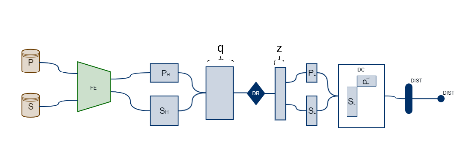
Figure 1: The figure shows the distance computation process discussed in the section 3.2. FE is the feature extractor/model from which high dimensional feature vectors $P_{H}$ and $S_{H}$ are obtained. The DR (dimensionality reduction) using PCA results in low dimensional representations $P_{L}$ and $S_{L}$ from q to z dimensions of the (n+m) images. Finally, the $I^{dist}$ and $O^{dist}$ are computed using the paiwise distance matrix shown in the DC(distance computation) block.

3.3 Performance Computation

We use F-score and perceptual quality (to resolve a few overlap boundary cases when we felt that the F-score is not discriminative) as the two main parameters to evaluate a model’s performance. The F-score of crack pixels computed by choosing a threshold that results in the highest F-score over all the images considered for evaluation; has been used as the performance metric. It is also known as Overall Dataset Score (ODS) and the computation is adapted from here. It is to be noted that the performance metric (ODS) is chosen with respect to the task in consideration i.e. segmentation and a suitable performance metric can be chosen based on the required tasks like classification, object detection, etc.

4 Experiments

4.1 Crack vs Non Crack Distinguishability

There is a significant difference in the visual representation of the crack and non-crack datasets, our goal is to show that the differences are captured by the selected pretrained models (namely SAM, CLIPSeg and ENet). To quantify these differences, we compute the $O^{dist}(S,P)$ (as discussed in section 3.2) of each of the secondary datasets $S$ from the primary dataset $P$ using these models.

These pretrained models can capture the global contexts as they are trained on large datasets having different backgrounds. This suggests that we can use the distance metric to distinguish different datasets. However, these pretrained models are not trained to perform crack segmentation (for more details, see section LABEL:saminf and LABEL:clipinf). Therefore, to understand the relationship between the crack datasets, we selected three architectures namely DC, UNet⁺⁺ and ADSAM to train on $P$ and computed the distances of the secondary crack datasets from $P$ along with the performance on these secondary datasets.

DC is trained using scripts provided here, UNet⁺⁺ is initialized with an EfficientNet-B3 backbone LABEL:efficientnet and trained with a multi-gpu setup using segmentation models pytorch LABEL:smp and pytorch lightning LABEL:plig and ADSAM is trained using the "base" version of SAM LABEL:sam. The training scripts for ADSAM can be found here.

4.2 Distance and Performance

The distinguishability of images within each crack dataset for DC, UNet⁺⁺ and ADSAM is analyzed. The performance of these models is computed on the secondary crack datasets $S$ ($S_{1},S_{2},S_{3}$ and $S_{4}$). Within the same dataset, a set of images can be closer to $P$ whereas another set of images can be farther from $P$. It is expected that the model performance will be better on the images closer to $P$ as compared to those that are farther. To validate the same, we perform the following analysis.

4.2.1 Intra Dataset Analysis

Firstly, we compute the $I^{dist}(S,P)$. The images are then sorted in ascending order of distances $I^{dist}(S,P)$ and divided into two equal parts based on the distance. The F-score ($F_{1}$, $F_{2}$), mean distances ($\mu_{1}$, $\mu_{2}$) and standard deviations($\sigma_{1}$, $\sigma_{2}$) of each part are computed. The same computation is repeated by splitting the dataset into 3 equal parts to show the difference in performance between the closest and farthest images of $S$ from $P$. A plot LABEL:udidx of sorted images vs distance from $P$ can be seen in the appendix.

$$\begin{split}\mu_{1}=\frac{1}{\frac{m}{2}}\sum_{j=1}^{\frac{m}{2}}I_{j}^{dist}(S,P)\\ \mu_{2}=\frac{1}{\frac{m}{2}}\sum_{j=\frac{m}{2}+1}^{m}I_{j}^{dist}(S,P)\\ \sigma_{1}=\frac{1}{m/2}\sum_{j=1}^{m/2}I_{j}^{dist}(S,P)-\mu_{1}\\ \sigma_{2}=\frac{1}{\frac{m}{2}}\sum_{j=\frac{m}{2}+1}^{m}I_{j}^{dist}(S,P)-\mu_{2}\\ \end{split}$$ (8)

Equation set 8: ($\mu_{1}$, $\mu_{2}$) and ($\sigma_{1}$, $\sigma_{2}$) are the means of the first half and second half of the sorted $I^{dist}(S,P)$. Computation can be performed for three parts similarly.

4.3 Model Adaptation

We perform an experiment by selecting $n$ (from P)+$q$ (from $S$) images ($n=\lvert P\rvert$ and $q\in\{1,3,7\}$) from each secondary dataset $S$. These datasets are used to train three models with different adaptations. The baseline models are herafter referred as M and the adapted models as M₁, M₃ and M₇ respectively. The F-score vs $I^{dist}(S,P)$ plots of these adapted models are compared with the baseline models i.e. the models trained on just $P$. For plotting purposes, we perform a moving average with a window size of $\lvert S\rvert/10$ on the F-scores and a min-max scaling on $I^{dist}(S,P)$. In min-max scaling, we scale a set of numbers x into a range of 0-1 by using the absolute minimum and maximum values of x and get $x_{scaled}=(x-x_{min})/(x_{max}-x_{min})$. The images were selected at a distance of 0.6-1 after the min-max scaling.

4.4 Model Understanding

To understand the behaviour of the models on images different from the crack images, we perform inference using the models (DC, UNet⁺⁺ and ADSAM trained on $P$) on the images from the BSDS500 LABEL:bsds500 dataset. The motivation is to observe the masks produced by these models and understand whether the model is actually predicting cracks or is predicting crack like features/edges from the images. If a model extracts crack like features from every image as cracks, it may give ambiguous distances. We also compute the distances obtained from a variety of models on scene-centric scenarios to understand the model behaviour on diverse range of scenes(see details in section LABEL:scene).

5 Results

The table 2 and figure 3 shows the distances computed from all the selected models (see details of the models in table 1). The non-crack datasets $S_{5}$ and $S_{6}$ are the farthest from $P$ for all the models except for DC where the model’s focus is on the edges present in the images (see figure 2).

Since there is a tradeoff between the precision and recall, we can decide the kind of model required for the task in hand. The figure 2 gives a good understanding on the behaviour of the models. In figure 2, the deepcrack model is more confident in detecting edge like structures compared to ADSAM and UNet⁺⁺. This suggests that ADSAM can be used for high precision and DC for high recall.

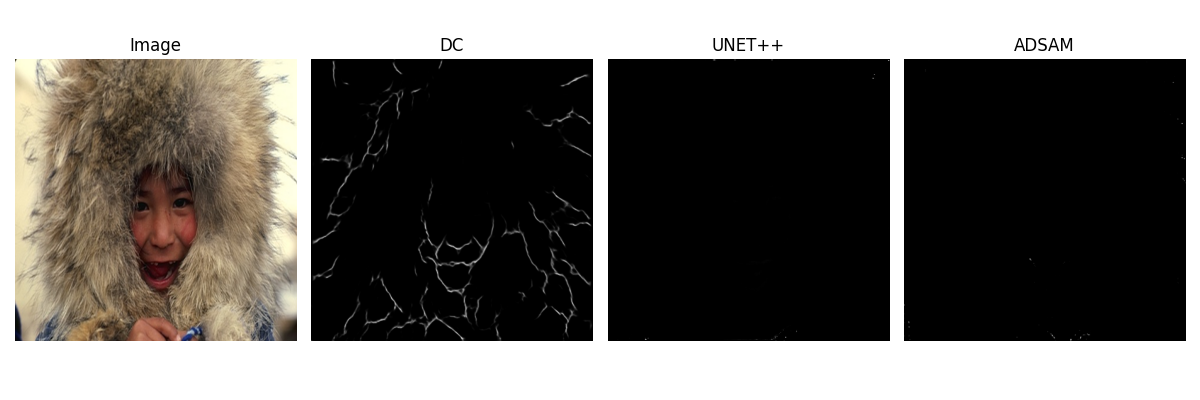
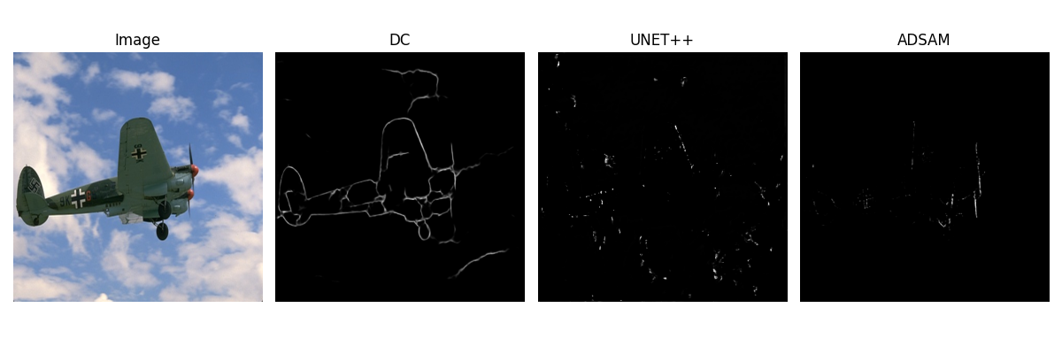
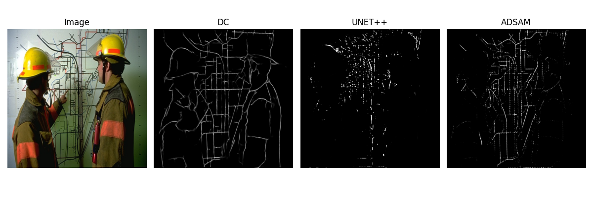
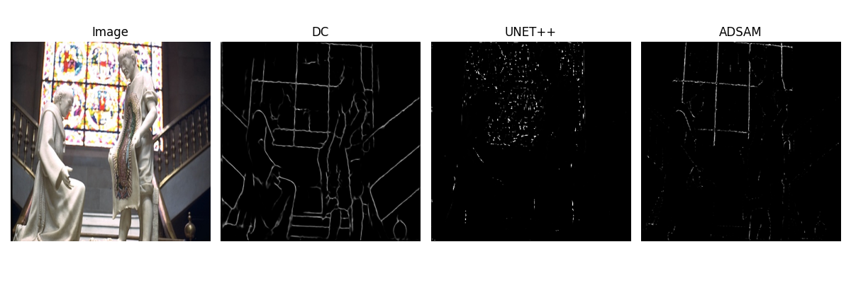
Figure 2: Shows (a) original image, (b) DC , (c) UNet⁺⁺ and (d) ADSAM outputs on the images from $S_{6}$. DC model focuses on specific features like edges.

The tables 3 for UNet⁺⁺ , 4 for DC and 5 for ADSAM show the F-score and mean distance obtained by the models on each part of each secondary crack dataset (see captions of the tables for more details). The tables 3(a) and 3(b) show that the performance is also similar for the first and second half on $S_{1}$, $S_{2}$ and $S_{3}$ but the performance first half is significantly higher than the second half for $S_{4}$. Overall, there is a decreasing trend with distances for the UNet⁺⁺ model. Similarly, the other two models also follow a decreasing trend in the performance with the distances which can be seen in the tables 4(a), 4(b), 5(a) and 5(b).

The figures 4, 5 and 6 show the F-score vs $I^{dist}(S,P)$ comparison for the models UNet⁺⁺, DC and ADSAM respectively. These plots show the model performance when trained on $P$, $P$ + 1 image from each secondary, $P$ + 3 images from each secondary and $P$ + 7 images from each secondary dataset. After the training of the models, we can see a significant improvement in the performance across datasets and images, thereby increasing the generalization of the models (see captions and figure 7 for additional details).

	$S_{1}$	$S_{2}$	$S_{3}$	$S_{4}$	$S_{5}$	$S_{6}$
SAM	0.149	0.145	0.164	0.134	0.213	0.195
CLIPSeg	0.135	0.134	0.142	0.153	0.236	0.199
ENet	0.153	0.153	0.159	0.163	0.188	0.183
$DC$	0.153	0.188	0.153	0.174	0.166	0.167
UNet++	0.056	0.069	0.063	0.054	0.465	0.293
ADSAM	0.166	0.152	0.163	0.148	0.193	0.178

Table 2: The table shows the scaled $O^{dist}(S,P)$. The numbers in each cell are obtained after dividing the $O^{dist}(S,P)$ by the sum of the corresponding row. The top 2 farthest distances for each model from $P$ are shown in bold.

i SAM

ii CLIPSeg

iii ENet

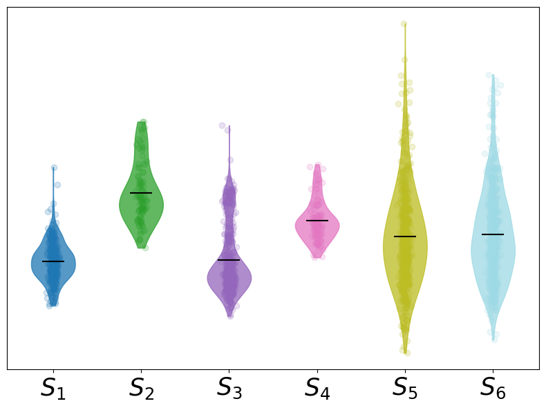
iv DC

v UNet⁺⁺

vi ADSAM

Figure 3: Shows the comparison of the violin plots (using  LABEL:plt) of $I^{dist}$ distribution of all the secondary datasets $S$ from $P$. The corresponding quantitative results can be seen in 2.

Dataset	$F(\mu,\sigma)[0-50\%]$	$F(\mu,\sigma)[50-100\%]$
$S_{1}$	0.483(0.2, 0.06)	0.444(0.54, 0.18)
$S_{2}$	0.567(0.24, 0.15)	0.606(0.79, 0.13)
$S_{3}$	0.353(0.19, 0.06)	0.316(0.48, 0.16)
$S_{4}$	0.241(0.03, 0.02)	0.061(0.4, 0.23)

(a) The table shows the comparison of the performance of first 50% and last 50% images.

Dataset	$F(\mu,\sigma)[0-33\%]$	$F(\mu,\sigma)[67-100\%]$
$S_{1}$	0.488(0.18, 0.05)	0.415(0.64, 0.13)
$S_{2}$	0.584(0.15, 0.09)	0.622(0.85, 0.1)
$S_{3}$	0.365(0.16, 0.04)	0.314(0.56, 0.13)
$S_{4}$	0.283(0.02, 0.01)	0.021(0.5, 0.17)

(b) The table shows the comparison of the performance of first 33% and last 33% images.

Table 3: The performance is computed using UNet⁺⁺ trained on $P$. Each cell in the tables represents the F-score(mean, standard deviation). See details in the section 4.2.1.

Dataset	$F(\mu,\sigma)[0-50\%]$	$F(\mu,\sigma)[50-100\%]$
$S_{1}$	0.346(0.21, 0.08)	0.318(0.42, 0.09)
$S_{2}$	0.432(0.25, 0.09)	0.464(0.62, 0.19)
$S_{3}$	0.461(0.16, 0.04)	0.391(0.42, 0.16)
$S_{4}$	0.625(0.24, 0.09)	0.58(0.56, 0.18)

(a) The table shows the comparison of the performance of first 50% and last 50% images.

Dataset	$F(\mu,\sigma)[0-33\%]$	$F(\mu,\sigma)[67-100\%]$
$S_{1}$	0.34(0.17, 0.07)	0.30(0.47, 0.1)
$S_{2}$	0.43(0.2, 0.08)	0.489(0.7, 0.16)
$S_{3}$	0.472(0.14, 0.04)	0.37(0.5, 0.14)
$S_{4}$	0.638(0.19, 0.07)	0.58(0.63, 0.17)

(b) The table shows the comparison of the performance of first 33% and last 33% images.

Table 4: The performance is computed using DC trained on $P$. Each cell in the tables represents the F-score(mean, standard deviation). See details in the section 4.2.1.

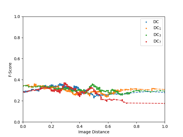
i $S_{1}$

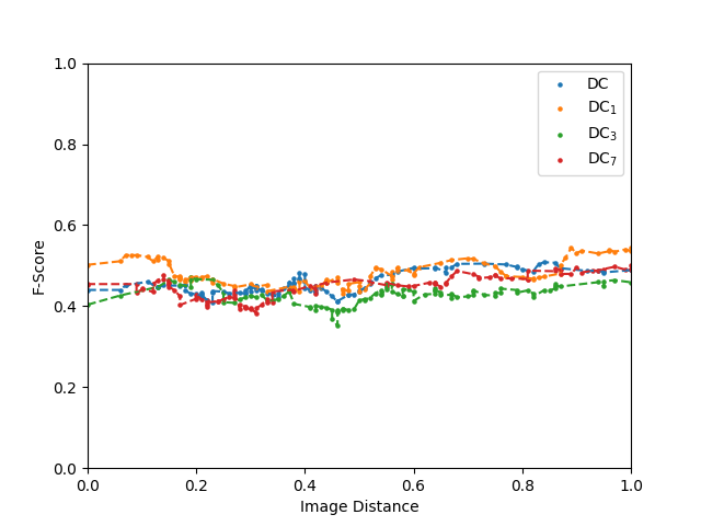
ii $S_{2}$

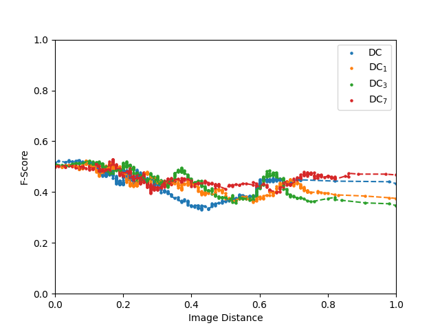
iii $S_{3}$

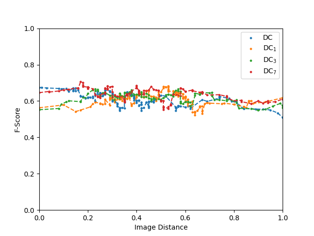
iv $S_{4}$

Figure 4: The figure shows the F-score vs $I^{dist}(S,P)$ plot for $S$. The results are computed using the DC model which was trained on $P+n,n\in\{0,1,3,7\}$ where n images are selected from each $S$.

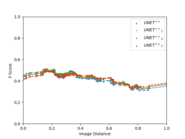
i $S_{1}$

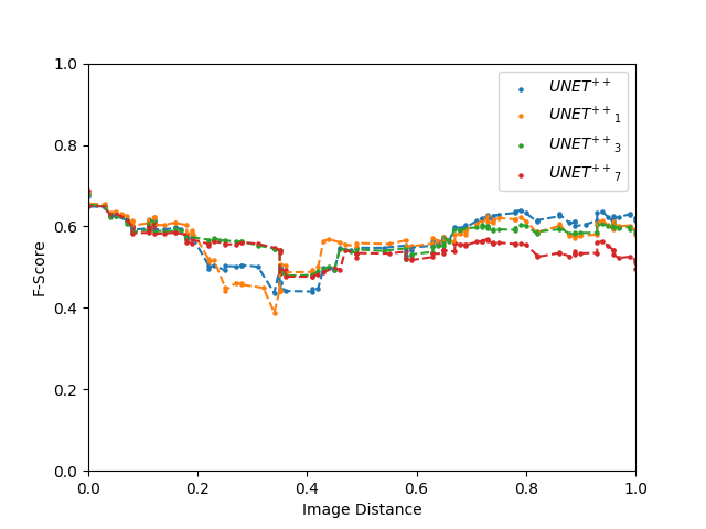
ii $S_{2}$

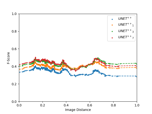
iii $S_{3}$

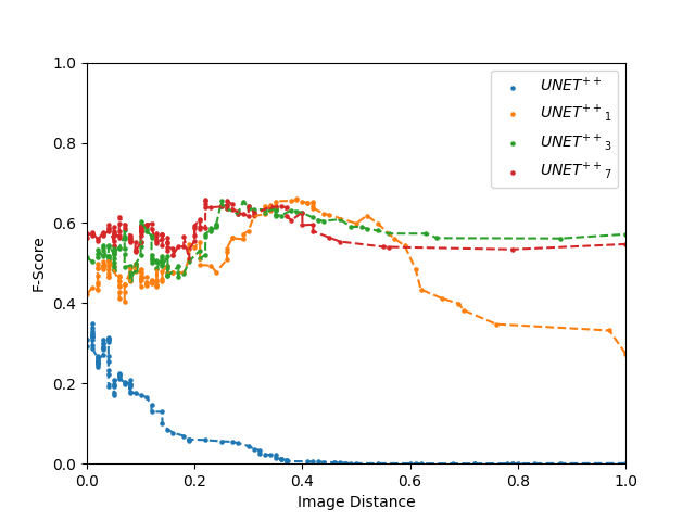
iv $S_{4}$

Figure 5: This figure shows the F-score vs $I^{dist}(S,P)$ plot for $S$. The results are computed using UNet⁺⁺ model which was trained on $P+n,n\in\{0,1,3,7\}$ where n images are selected from each $S$.

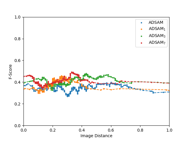
i $S_{1}$

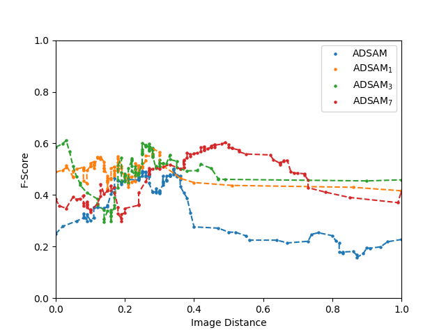
ii $S_{2}$

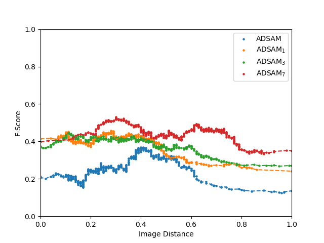
iii $S_{3}$

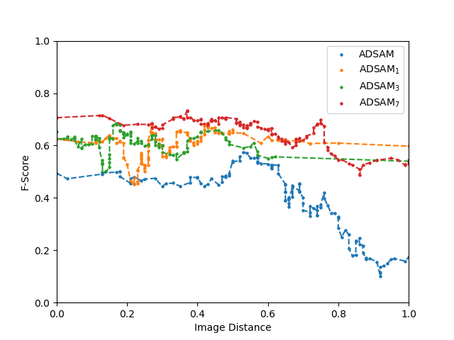
iv $S_{4}$

Figure 6: This figure shows the F-score vs $I^{dist}(S,P)$ plot for $S$. The results are computed using the ADSAM model which was trained on $P+n,n\in\{0,1,3,7\}$ where n images are selected from each $S$.

Dataset	$F(\mu,\sigma)[0-50\%]$	$F(\mu,\sigma)[50-100\%]$
$S_{1}$	0.388(0.23, 0.09)	0.4(0.51, 0.14)
$S_{2}$	0.392(0.2, 0.08)	0.375(0.56, 0.24)
$S_{3}$	0.249(0.19, 0.07)	0.292(0.47, 0.14)
$S_{4}$	0.471(0.44, 0.17)	0.33(0.79, 0.1)

(a) The table shows the comparison of the performance of first 50% and last 50% images.

Dataset	$F(\mu,\sigma)[0-33\%]$	$F(\mu,\sigma)[67-100\%]$
$S_{1}$	0.383(0.184, 0.07)	0.405(0.584, 0.13)
$S_{2}$	0.37(0.16, 0.07)	0.29(0.654, 0.21)
$S_{3}$	0.226(0.153, 0.05)	0.293(0.533, 0.12)
$S_{4}$	0.462(0.353, 0.15)	0.291(0.842, 0.07)

(b) The table shows the comparison of the performance of first 33% and last 33% images.

Table 5: The performance is computed using ADSAM trained on $P$. Each cell in the tables represents the F-score(mean, standard deviation). See details in the section 4.2.1.

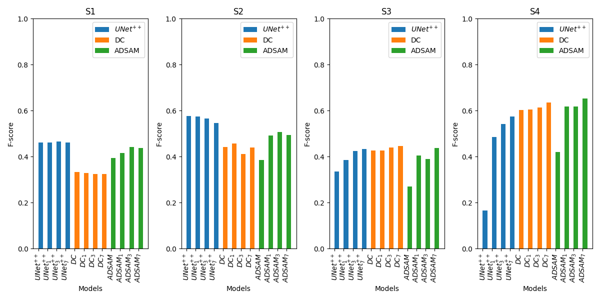
Figure 7: The figure shows the performance (F-score) of the M, M₁, M₃ and M₇ models on the secondary datasets, $S$.

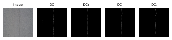
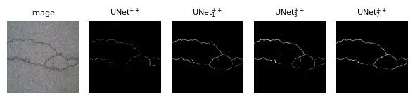
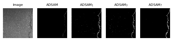
Figure 8: Shows original image, M, M₁, M₃ and M₇ outputs on different datasets. The input image for DC and UNet⁺⁺ is from $S_{4}$ and from $S_{3}$ for ADSAM. The titles of each figure (except the crack images from the dataset) show the name of model used for inference.

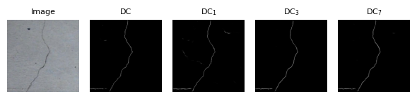
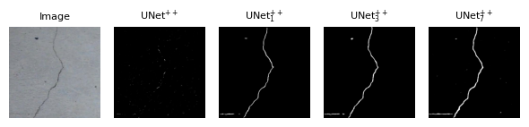
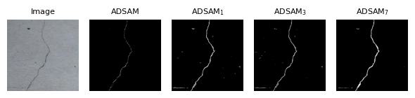
Figure 9: Shows original image, Model, Model₁, Model₃ and Model₇ outputs on EUGEN MULLER LABEL:kagglecrack dataset. The titles of each figure (except the crack images from the dataset) show the name of model used for inference.

6 Observations

The results in the figures 4, 5 and 6 show that the performance of models trained on $P$ decreases as the distance increases. This gives a motivation to select a few images ($\{1,3,7\}$) from each of the secondary crack datasets and train the models by adding the selected images into the training data. The trained models seem to generalize on all secondary datasets which can be seen in the figures 4, 5 and 6. Fewer number of images are selected to reduce the labelling cost that can also improve the generalization of the models on different unseen datasets LABEL:truedeep.

The majority of $S_{4}$ images with an $I^{dist}(S_{4},P)$ exceeding $0.4$ for the baseline UNet$++$ model and $0.5$ for the baseline $ADSAM$ model exhibit poor F-scores (as indicated by the blue line in figs. 5 (iv) and 6 (iv)). As these models are adapted, there is a significant performance enhancement (orange, green and red lines in figs. 5 (iv), 6 (iv)). Whereas, the performance for the DC model is almost same on all images in $S_{4}$ for the baseline and adapted models. As there is a tradeoff between crack and background prediction, some models produce high recall results and others, high precision. Therefore, some models require crack expression whereas others require suppression. The suppression analysis, discussed in the section LABEL:back in the appendix, improves depth of our generalization study.

It’s noticeable that as the distance from the training dataset increases, the performance of most models tends to decrease. This trend suggests that images closer to the training dataset generally exhibit better model performance, while those farther away tend to have lower performance. This decrease in performance can be attributed to the models being optimized for the training data, whereas unseen images might contain new patterns not covered during training. The F-score may not always be an accurate estimate of the performance and the ambiguity in some cases can be resolved using a different metric such as perceptual quality.

If the performance plot vs distance is a near-horizontal line parallel to the x-axis, that indicates that the model is consistently performing well across the images (generalizes well). In this case, the model has already reached a satisfactory performance and adding new images from $S$ into the training set might not have a significant effect on the generalization of the model. However, the baseline performance can be further improved using additional set of images with a potential risk of overfitting. The amount of data required to achieve a near-horizontal line and the stability in performance metric across multiple unseen datasets are important factors that can help in the model selection.

The figures 8 and 9 show the qualitative improvement in performance of the adapted models over the baseline models i.e. the models only trained on $P$. The quality of predictions is in the order $M<M_{1}<M_{3}<M_{7}$ where M is the model used. The same trend can be observed in figure 9 where the is improvement is shown on a completely blind dataset i.e. dataset that is not used for model training and adaptation. This shows that the overall adaptability of the models is increasing. The baseline DC model performs better than UNet$++$ and ADSAM but shows little improvement with adaptation whereas UNet$++$ and ADSAM show significant improvements with adaptation. Overall, the improvement in crack predictions using model adaptation suggests that there is an improvement in model generalization across multiple datasets. This can be also seen in the figures 4, 5 and 6, where the F-score vs $I_{dist}$ curve for the adapted models is near parallel to the x-axis. The improvement is not significant if the model is already performing consistently across unseen datasets which is the case for the DC model.

7 Conclusion

Our study analyzes multiple datasets to demonstrate that the performance of the models can be related to the proposed distance metrics (see figures 4, 5 and 6). This helps in improving an existing model with few images (improving generalization) and in turn, reducing the labeling and training cost while avoiding overfitting. We have shown that guiding the model with only a few images (see figure 7) from each of the secondary datasets can improve its performance significantly.

Our approach helps in explaining the behaviour of the models that can be seen in figures 2, 3, 4, 5 , 6 and 9.

We also study the distances on scene-centric and person re-identification tasks (see details in sections LABEL:scene and LABEL:personreid in the Appendix).

7.1 Future Scope

The proposed approaches can be extended to explain model behaviour on other deep learning tasks by selecting our distance metrics (see section 3.2) and a suitable performance metric (see section 3.3) for that task. As the feature representations from the deep learning models express the input features, the applicability of the proposed distance metrics can be tested different data domains.

The approaches can be further tested in real-world environments for examining the robustness and adaptability when faced with dynamic data distributions and generalization capabilities in the field. Research in this direction can have significant contributions in the applications that necessitate the selection of diverse datasets to train models capable of generalizing to new datasets.

Furthermore, theoretical aspects relating the distances to the model performance and generalization can also be studied.

8 Acknowledgement

We would like to thank GE Research for providing us with the resources and a conducive environment that made this research possible.