Data-driven robust MPC of tiltwing VTOL aircraft

Abstract

This paper investigates robust tube-based Model Predictive Control (MPC) of a tiltwing Vertical Take-Off and Landing (VTOL) aircraft subject to wind disturbances and model uncertainty. Our approach is based on a Difference of Convex (DC) function decomposition of the dynamics to develop a computationally tractable optimisation with robust tubes for the system trajectories. We consider a case study of a VTOL aircraft subject to wind gusts and whose aerodynamics is defined from data.

1 Introduction

Urban Air Mobility (UAM) has a potential to transform transportation of people and goods in congested cities [1] while potentially reducing ground traffic. A key enabler of this technology is a class of zero carbon emission eVTOL aircraft concepts [2], many based on tiltrotor, tiltduct or tiltwing vehicle configurations powered by batteries or by making use of zero carbon fuel like hydrogen [3]. However, the lower energy density of energy storage options relative to liquid carbon based fuels restrict the operational range, hover time and cruise speeds. Additionally such concepts require transition between vertical and horizontal flight further complicating operational scenarios. Consequently limited energy and transition envelope constraints impede the throughput of flight operations by limiting the number of flights, timely allocation of landing slots, duration of holding patterns in hover, and separation between vehicles. To maximise throughput it is clear that both the energy spent in a non-wing-borne flight phase and the time and space needed to transition between thrust-borne and wing-borne flight should be minimised.

This paper proposes a robust control methodology for transitions of VTOL aircraft between wing-borne and thrust-borne flight phases in the presence of wind gusts, model uncertainty and state constraints. We explore a Model Predictive Control framework due to its potential to outperform classical control architectures by optimising future control sequences with respect to a specified objective (usually minimum time or minimum energy transition) with explicit constraint handling using a model of the vehicle. This methodology can also provide guarantees of robustness to model uncertainty and external disturbances [4]. Although we develop here MPC policies for a generic class of tiltwing aircraft, the ideas presented in this paper are equally applicable to tilt rotors and tilt ducts.

Various approaches have been proposed to address this problem. In [5], a cascaded PID control architecture was proposed for the transition of a prototype tiltrotor VTOL aircraft. The transition is achieved through smooth scheduling functions of the forward velocity or tilt angle, and the simulation results are supported by flight test results. Modeling, control and flight testing for the transition of a tiltwing aircraft are achieved in [6], extending the P-PID structure from the PX4 open-source software with feedback linearisation, gain scheduling and model-based control allocation. A gain-scheduled LQR control architecture is presented in [7] for the transition of a tandem tiltwing aircraft in the presence of moderate wind gusts. Instabilities were observed for wind gusts of intensity larger than $5$\mathrm{m}\mathrm{/}\mathrm{s}$$ during transitions, which limits the viability of the approach in the presence of wind in realistic conditions.

Recent advances in robust tube-based MPC allow robust control of nonlinear systems whose dynamics can be represented as a difference of convex functions [8]. The main idea is to successively linearise the dynamics around predicted trajectories and treat linearisation errors as bounded disturbances. Because the linearised functions are convex, so are their linearisation errors, and since these errors are maximised at the boundary of the domain on which they are evaluated, they can therefore be bounded tightly. The trajectories of model states are thus bounded tightly by a sequence of sets (known as a tube [4]) defined by convex inequalities. Although very efficient, the scope of applicability is initially limited to systems with convex dynamics. However, we show that if the dynamics are sufficiently regular, techniques from difference of convex (DC) decomposition of polynomials [9] can be used to represent the VTOL nonlinear dynamics as a difference of convex functions, which allows the powerful approach in [8] to be used. The dynamics need not be derived using first principles modelling; we employ a mixture of data-based and physical models. The proposed approach is the culmination of our work [10, 11] on convex trajectory optimisation of VTOL aircraft.

The specific contributions of this research over earlier work are as follows: i) we propose a computationally tractable, optimal, robust control architecture for VTOL aircraft subject to additive disturbance and model uncertainty; ii) we combine DC decomposition with robust tube-based MPC and demonstrate the applicability and generalisability of the procedure in [8]; iii) we show that our technique also applies when parts of the model are defined from data.

This paper is organised as follows. We start by developing a mathematical model of a tiltwing VTOL aircraft subject to wind disturbance in Section 2.1. In Section 3, we formulate the MPC optimisation problem and leverage a DC decomposition of the nonlinear dynamics to construct robust tubes for the state trajectories. Section 4 discusses simulation results obtained for a case study based on the Airbus A³ Vahana. Section 5 presents conclusions.

2 Modelling

2.1 Assumptions

We assume a flat earth model and consider trajectory optimisation in the longitudinal plane alone. Tiltwing aircraft are considered (see Figure 1), with one or more wing surfaces carrying thrust effectors that can be rotated by an actuator through 90 degrees as the aircraft transitions between wing-borne and thrust-borne flight. We further assume classical inner/outer loop flight control laws for stabilisation of aircraft attitude with time-scale separation, so that the closed loop pitch dynamics are much faster than those of the desired flight path and tiltwing actuation. Consequently the pitch angle $\theta$ (defined here as the angle of the fuselage axis from horizontal earth plane) is assumed to be maintained at all times by the attitude control loop at a constant reference angle $\theta^{r}=0$.

2.2 Equations of motion

Consider a longitudinal point-mass model of a tiltwing VTOL aircraft equipped with propellers (Figure 1) subject to a wind gust disturbance. The Equations Of Motion (EOM) with respect to inertial frame $O_{XZ}$ are given by

$$\dot{X}=V_{x},\quad\dot{Z}=V_{z},$$ (1)

$$m\dot{V}_{x}=\underbrace{T\cos{(\alpha+\gamma)}-D\cos{\gamma}-L\sin{\gamma}}_{f_{1}}+W_{x},$$ (2)

$$m\dot{V}_{z}=\underbrace{-T\sin{(\alpha+\gamma)}+D\sin{\gamma}-L\cos{\gamma}+mg}_{f_{2}}+W_{z},$$ (3)

where $T$ is the thrust magnitude, $L$, $D$ are the lift and drag forces, $V_{x},V_{z}$ the components of the aircraft velocity in the inertial frame $V=\sqrt{V_{x}^{2}+V_{z}^{2}}$, $\alpha$ is the angle of attack, $\gamma=-\arcsin(V_{z}/V)$ is the flight path angle (defined as the angle of the velocity vector from horizontal), and $(X,Z)$ the position in inertial frame. Wind gusts are modelled by additive bounded disturbances $W_{x}$ and $W_{z}$, which are assumed to lie at all times within known bounds.

The dynamics of the rotating wing are given by

$$J_{w}\dot{\zeta}=M,\quad\dot{i}_{w}=\zeta,$$ (4)

where $J_{w}$ is the rotational inertia of the wing (about the $y$-axis), $M$ is the total torque delivered by the tilting actuators, $\zeta$ is the tiltwing rate and $i_{w}$ is the tiltwing angle. The angles $i_{w}$, $\theta$, $\alpha$ and $\gamma$ are related by (see Figure 1)

$$i_{w}+\theta=\alpha+\gamma.$$ (5)

From momentum theory, the propeller generates an induced speed $v_{i}$ that is implicitly defined by

$$\rho An(V\cos{\alpha}+v_{i})(k_{w}v_{i})-T=0,$$

where $\rho$ is the air density, $A$ the rotor disk area, $n$ the number of propellers, and $k_{w}\approx 2$ [10]. The effective (blown) velocity $V_{e}$ and effective (blown) angle of attack $\alpha_{e}$ seen by the wing due to the effect of the propeller wake on the wing are given by

$$V_{e}\cos{\alpha_{e}}=V\cos{\alpha}+k_{w}v_{i},$$ (6)

$$V_{e}\sin{\alpha_{e}}=V\sin{\alpha},$$ (7)

$$V_{e}^{2}=V^{2}+\frac{2T}{\rho An}.$$ (8)

The total lift and drag are modeled as the weighted sum of the blown and unblown terms as follows

$$L=\tfrac{1}{2}\lambda\rho SC_{L}(\alpha_{e})V_{e}^{2}+\tfrac{1}{2}(1-\lambda)\rho SC_{L}(\alpha)V^{2},$$ (9)

$$D=\tfrac{1}{2}\lambda\rho SC_{D}(\alpha_{e})V_{e}^{2}+\tfrac{1}{2}(1-\lambda)\rho SC_{D}(\alpha)V^{2},$$ (10)

where $S$ is the wing area, $\lambda$ is a weighting term representing the portion of the wing in the wake, and $C_{L}$ and $C_{D}$ are lift and drag coefficients. To illustrate the approach we define $C_{L}$ and $C_{D}$ using data derived from the Tangler-Ostowari post-stall model [12] (see Figure 2), which determines lift and drag forces over a wide range of $\alpha$ and $\alpha_{e}$ values as the wing operates at high angles of attack during transitions.

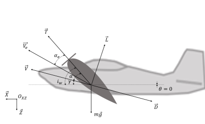
Figure 1: Force and velocity definitions for a VTOL aircraft.

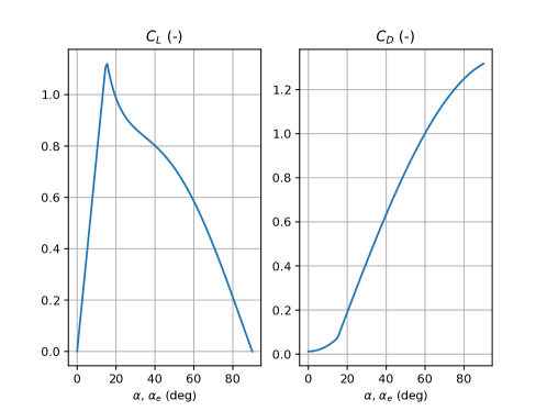
Figure 2: Lift and drag coefficients as a function of angle of attack.

2.3 Constraints

For the problem considered in this paper we assume that the gust disturbances $W_{x},W_{z}$ in the forward and vertical directions are bounded: $W_{i}\in[\underline{W}_{i},\overline{W}_{i}]$ for $i=x,z$. Since wing tilting actuators have finite torque capacity we also assume bounded wing acceleration/deceleration rates given by $\underline{M}$ and $\overline{M}$. To ensure sensible trajectories for passenger comfort and g-loads, we further introduce constraint limits on horizontal ($\dot{V}_{x}$) and vertical ($\dot{V}_{z}$) accelerations. Finally, constraints on thrust range, tilt angle range and absolute velocities can all be expressed in the compact form as input and state constraints [10],

$$\underline{V}_{x}\leq V_{x}\leq\overline{V}_{x},\quad\underline{V}_{z}\leq V_{z}\leq\overline{V}_{z},\quad 0\leq T\leq\overline{T},\quad\underline{i}_{w}\leq i_{w}\leq\overline{i}_{w},$$ (11)

$$V_{x}(t_{0})=V_{x,0},\quad V_{z}(t_{0})=V_{z,0},\quad i_{w}(t_{0})=i_{0},$$ (12)

$$\underline{W}_{x}\leq W_{x}\leq\overline{W}_{x},\quad\underline{W}_{z}\leq W_{z}\leq\overline{W}_{z},$$ (13)

$$\underline{a}\leq\dot{V}_{x}\leq\overline{a},\quad\underline{a}\leq\dot{V}_{z}\leq\overline{a},$$ (14)

$${\underline{M}}/{J_{w}}\leq\ddot{i}_{w}\leq{\overline{M}}/{J_{w}}.$$ (15)

3 Robust MPC formulation

We now introduce a robust predictive control law for the system presented in Section 2.1. Assuming we are only concerned with velocity control, the states $(X,Z)$ can be computed a posteriori via (1) and thus eliminated from the analysis. Moreover, combining equations (2)-(10), we can further eliminate the flight path angle, angle of attack, and tiltwing rate from the formulation and express the dynamics with only two states $V_{x},V_{z}$ and two inputs $i_{w},T$ as follows

$$m\dot{V_{x}}=f_{1}(V_{x},V_{z},i_{w},T)+W_{x},$$ (16)

$$m\dot{V_{z}}=f_{2}(V_{x},V_{z},i_{w},T)+W_{z},$$ (17)

where $i_{w}$ is now an input constrained by its second order derivative (see equation 15).

To setup the MPC problem we use the trajectory constraints given by (11)-(15) together with the terminal set for the velocities[8]

$$\Biggl{\|}\Biggl{[}\begin{matrix}{V}_{x}(t_{f})-V_{x}^{r}(t_{f})\\ {V}_{z}(t_{f})-V_{z}^{r}(t_{f})\end{matrix}\Biggr{]}\Biggr{\|}_{\hat{Q}}^{2}\leq\hat{\gamma},$$ (18)

where the notation $\cdot^{r}$ was used to denote a reference to be tracked, $t_{f}$ is a fixed terminal time, $\hat{\gamma}$ and $\hat{Q}\succ 0$ are respectively a terminal set bound and penalty matrix that can be computed following Appendix of [8]. Note that equation (18) enforces the conditions: $|V_{x}(t_{f})-V_{x}^{r}(t_{f})|\leq\delta^{V}$, $|V_{z}(t_{f})-V_{z}^{r}(t_{f})|\leq\delta^{V}$, $|i_{w}(t_{f})-i_{w}^{r}(t_{f})|\leq\delta^{i_{w}},\quad|T(t_{f})-T^{r}(t_{f})|\leq\delta^{T}$, where $\delta^{V},\delta^{i_{w}},\delta^{T}$, are terminal sets bounds.

The control objective is to achieve tracking of a reference trajectory $V_{x}^{r},V_{z}^{r},i_{w}^{r},T^{r}$ while rejecting the wind disturbances $W_{x},W_{z}$ acting on the system. To do so, at each time step, we could compute a receding horizon control law that minimises the worst case quadratic objective defined for $Q_{x}\succ 0$, $Q_{u}\succ 0$ by

$$J(u)=\max_{\begin{subarray}{c}W_{x}\in[\underline{W}_{x},\overline{W}_{x}]\\ W_{z}\in[\underline{W}_{z},\overline{W}_{z}]\end{subarray}}\Biggl{\{} \Biggl{\|}\Biggl{[}\begin{matrix}V_{x}(i_{w}(t_{f}),T(t_{f}),W_{x}(t_{f}),W_{z}(t_{f}))-V_{x}^{r}(t_{f})\\ V_{z}(i_{w}(t_{f}),T(t_{f}),W_{x}(t_{f}),W_{z}(t_{f}))-V_{z}^{r}(t_{f})\end{matrix}\Biggr{]}\Biggr{\|}_{\hat{Q}}^{2}$$ (19)

$$+\int_{t_{0}}^{t_{f}}\Biggl{\|}\Biggl{[}\begin{matrix}V_{x}(i_{w}(t),T(t),W_{x}(t),W_{z}(t))-V_{x}^{r}(t)\\ V_{z}(i_{w}(t),T(t),W_{x}(t),W_{z}(t))-V_{z}^{r}(t)\end{matrix}\Biggr{]}\Biggr{\|}_{Q_{x}}^{2}+\ \ \Biggl{\|}\Biggl{[}\begin{matrix}i_{w}(t)-i_{w}^{r}(t)\\ T(t)-T^{r}(t)\end{matrix}\Biggr{]}\Biggr{\|}_{Q_{u}}^{2}\,\mathrm{d}t\Biggr{\}}$$

subject to (11)-(18). Note that the states are uncertain and that the state trajectories in the objective are computed as the worst case realisation of the time-varying gust disturbances $W_{x},W_{z}$. We would then apply the first element of the obtained optimal control sequence, update the current state and input and repeat the process at each time step. Since the model includes the nonlinear functions $f_{1}$ and $f_{2}$ and that the state is uncertain, computing the control law would require solving a min-max Nonlinear Program (NLP) which is intractable in practice. In what follows, we introduce a DC decomposition of these nonlinear functions in order to obtain a computationally efficient implementation of the robust MPC problem.

3.1 DC decomposition

Motivated by the fact that convex functions can be bounded tightly by convex and linear inequalities (as in [8]), we seek DC decompositions of $f_{1},f_{2}$: $f_{1}=g_{1}-h_{1}$ and $f_{2}=g_{2}-h_{2}$, where $g_{1},h_{1},g_{2},h_{2}$ are convex. A DC decomposition always exists if $f_{1},f_{2}\in\mathcal{C}^{2}$ [13] and can be precomputed offline. A similar procedure was first presented in [11] and follows an idea from [9] on DC decomposition of nonconvex polynomials using algebraic techniques. In what follows we detail the procedure for the DC decomposition of a general function $f$ (and hence its applicability to $f_{1}$ and $f_{2}$):

3.1.1 Fit polynomial to data

Assume that the nonlinear model $f$ can be approximated arbitrarily closely by a polynomial of degree $2d$ in Gram form such that $f\approx y(x)^{\top}Py(x)$, where $P=P^{\top}$ is the Gram matrix and $y=[1,x_{1},x_{2},\dots,x_{n},x_{1}x_{2},\dots,x_{n}^{d}]^{\top}$ is a vector of monomials of degree up to $d$ ($y$ has size $C^{|x|}_{d+|x|}$). Generate $N_{s}$ samples $F_{s}=f(x_{s}),\forall s\in[1,...,N_{s}]$ of the nonlinear model and solve the following least squares problem:

$$\mathcal{LS}:\quad\min_{\begin{subarray}{c}P\end{subarray}}\quad\sum_{s=0}^{N_{s}}\lVert F_{s}-y(x_{s})^{\top}Py(x_{s})\rVert^{2}_{2},\quad\text{ s.t.}\quad P=P^{\top}.$$

3.1.2 Compute the Hessians of the decomposition

Let $g(x)\approx y(x)^{\top}Qy(x)$ and $h(x)\approx y(x)^{\top}Ry(x)$ be convex polynomials such that their Hessians $d^{2}g(x)/dx^{2}=y(x)^{\top}H_{g}y(x)$ and $d^{2}h(x)/dx^{2}=y(x)^{\top}H_{h}y(x)$ are Positive Semi-Definite (PSD). Finding $Q,R$ such that $P=Q-R$ and $h(x)$, $g(x)$ are convex reduces to solving the following Semi Definite Program (SDP)

$$\mathcal{SDP}:\max_{\begin{subarray}{c}Q,\sigma\end{subarray}} \sigma\quad\text{ s.t.} H_{g}(Q)\succeq\sigma I,\quad H_{h}(Q)\succeq\sigma I,$$

with $\forall i,j$

$$[H_{g}]_{ij}={D}_{j,i}^{\top}Q+Q{D}_{i,j}+{D}_{i}^{\top}QD_{j}+{D}_{j}^{\top}QD_{i},$$

$$[H_{h}]_{ij}={D}_{j,i}^{\top}(Q-P)+(Q-P){D}_{i,j}+{D}_{i}^{\top}(Q-P)D_{j}+{D}_{j}^{\top}(Q-P)D_{i},$$

where $I$ is the identity matrix of compatible dimensions, $D_{i}$ is a matrix of coefficients such that $dy/d{x_{i}}=D_{i}y$ and $D_{i,j}=D_{i}D_{j}$.

3.2 Successive convex programming tube MPC for DC systems

The nonlinear dynamics in (16)-(17) can now be expressed in a DC form as follows

$$m\dot{V_{x}}=g_{1}(V_{x},V_{z},i_{w},T)-h_{1}(V_{x},V_{z},i_{w},T)+W_{x},$$ (20)

$$m\dot{V_{z}}=g_{2}(V_{x},V_{z},i_{w},T)-h_{2}(V_{x},V_{z},i_{w},T)+W_{z},$$ (21)

and the DC-TMPC algorithm presented in [8] can be applied to the system.

In what follows we will exploit the convexity properties of the functions $g_{1},h_{1},g_{2},h_{2}$ in (20)-(21) to approximate the dynamics by a set of convex inequalities with tight bounds on the state trajectories. To do so, we linearise the dynamics successively around feasible guessed trajectories and treat the linearisation error as a bounded disturbance [8]. We use the fact that the linearisation error of a convex (resp. concave) function is also convex (resp. concave) and can thus be bounded tightly. This allows us to construct a robust optimisation using the tube-based MPC framework [4], and to obtain solutions that are robust to the model error introduced by the linearisation (i.e. model uncertainty) and to wind gusts (i.e. exogeneous additive disturbances).

The DC-TMPC framework is based on the following ingredients:

3.2.1 Parameterisation of the control input

We start by assuming the following two-degree of freedom parameterisation of the control inputs as follows [4]

$$i_{w}=\mu+K_{i_{w}}(V_{x}-V_{x}^{\circ})+K_{i_{w}}^{\prime}(V_{z}-V_{z}^{\circ}),$$

$$T=\tau+K_{T}(V_{x}-V_{x}^{\circ})+K_{T}^{\prime}(V_{z}-V_{z}^{\circ}),$$

where $V_{x}^{\circ},V_{z}^{\circ}$ are guess trajectories for the states, $\mu$, $\tau$ are feedforward terms (solution of the MPC optimisation stated in Section 3.3) and $K_{i_{w}},K_{i_{w}}^{\prime},K_{T},K_{T}^{\prime}$ are feedback gains to be computed e.g. by solving a LQR problem for the linearised nominal ($W_{x},W_{z}=0$) system (20)-(21). Note that $g_{1},h_{1},g_{2},h_{2}$ defined in (20)-(21) are now functions of $V_{x},V_{z},\mu,\tau$.

3.2.2 Successive linearisations

We assume the existence of a set of feasible guess trajectories $V_{x}^{\circ},V_{z}^{\circ},\mu^{\circ},\tau^{\circ}$ for (20)-(21) and successively linearise the dynamics around the guessed trajectories. The Taylor series expansion of the nonlinear dynamics is given by $\forall i\in\{1,2\}$

$$g_{i}=\lfloor g_{i}\rfloor_{(V_{x}^{\circ},V_{z}^{\circ},\mu^{\circ},\tau^{\circ})}+\lceil g_{i}\rceil_{(V_{x}^{\circ},V_{z}^{\circ},\mu^{\circ},\tau^{\circ})},$$

$$h_{i}=\lfloor h_{i}\rfloor_{(V_{x}^{\circ},V_{z}^{\circ},\mu^{\circ},\tau^{\circ})}+\lceil h_{i}\rceil_{(V_{x}^{\circ},V_{z}^{\circ},\mu^{\circ},\tau^{\circ})},$$

where the notation $\lfloor f\rfloor_{x^{\circ}}=f(x^{\circ})+\nabla f^{\top}(x^{\circ})(x-x^{\circ})$ stands for the Jacobian linear approximation of $f$ around $x^{\circ}$ and $\lceil f\rceil_{x^{\circ}}$ the corresponding linearisation error. After each iteration of the algorithm, the guessed trajectories are updated with the solution of the MPC optimisation and a new pass is initiated by linearising the dynamics around the new estimate.

3.2.3 Parameterisation of the uncertainty sets

We assume that the uncertain state trajectories $V_{x},V_{z}$ lie within “tubes” whose cross-sections are parameterised by means of elementwise bounds $V_{x}\in[\underline{V}_{x},\overline{V}_{x}],V_{z}\in[\underline{V}_{z},\overline{V}_{z}]$, which are optimisation variables, see Figure 3.

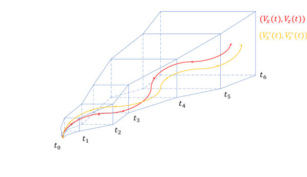
(a) Tube

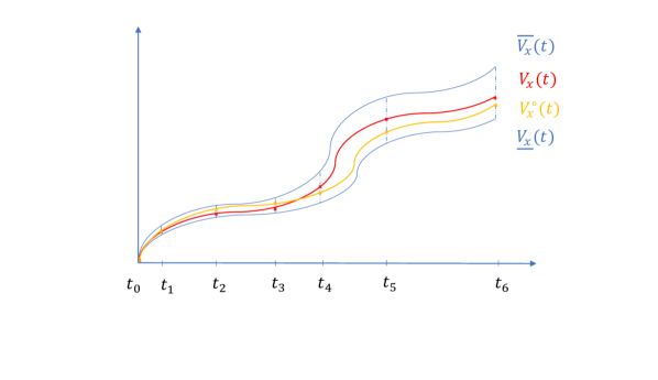
(b) Tube for $V_{x}$ only

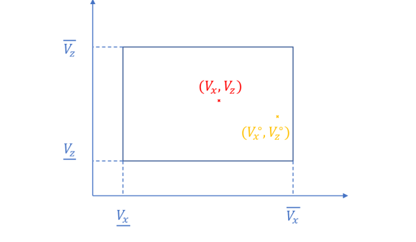
(c) Tube cross section

Figure 3: Schematic visualisation of the tube. The uncertain state trajectory (red) lies within a tube (blue) centred around the nominal trajectory (orange), sampled at various time steps (3(a)). Also shown is the tube evolution for state $V_{x}$ only (3(b)) and a snapshot of the tube cross section at an arbitrary time (3(c)).

3.2.4 DC properties of dynamics

By convexity of $g_{1},g_{2},h_{1},h_{2}$, the associated linearisation errors are necessarily convex and take their maximum on the boundary of the set over which the functions are constrained. Moreover, by definition, their minimum on this set is zero (Jacobian linearisation). It follows that the bounds on the states dynamics satisfy the following convex inequalities

$$m\dot{\overline{V_{x}}}\geq\max_{\begin{subarray}{c}V_{x}\in\{\underline{V}_{x},\overline{V}_{x}\},V_{z}\in\{\underline{V}_{z},\overline{V}_{z}\}\end{subarray}}\bigl{\{}g_{1}(V_{x},V_{z},\mu,\tau)-\lfloor h_{1}\rfloor_{(V_{x}^{\circ},V_{z}^{\circ},\mu^{\circ},\tau^{\circ})}(V_{x},V_{z},\mu,\tau)+\overline{W}_{x}\bigr{\}},$$ (22)

$$m\dot{\overline{V_{z}}}\geq\max_{\begin{subarray}{c}V_{x}\in\{\underline{V}_{x},\overline{V}_{x}\},V_{z}\in\{\underline{V}_{z},\overline{V}_{z}\}\end{subarray}}\bigl{\{}g_{2}(V_{x},V_{z},\mu,\tau)-\lfloor h_{2}\rfloor_{(V_{x}^{\circ},V_{z}^{\circ},\mu^{\circ},\tau^{\circ})}(V_{x},V_{z},\mu,\tau)+\overline{W}_{z}\bigr{\}},$$ (23)

$$m\dot{\underline{V_{x}}}\leq\min_{\begin{subarray}{c}V_{x}\in\{\underline{V}_{x},\overline{V}_{x}\},V_{z}\in\{\underline{V}_{z},\overline{V}_{z}\}\end{subarray}}\bigl{\{}-h_{1}(V_{x},V_{z},\mu,\tau)+\lfloor g_{1}\rfloor_{(V_{x}^{\circ},V_{z}^{\circ},\mu^{\circ},\tau^{\circ})}(V_{x},V_{z},\mu,\tau)+\underline{W}_{x}\bigr{\}},$$ (24)

$$m\dot{\underline{V_{z}}}\leq\min_{\begin{subarray}{c}V_{x}\in\{\underline{V}_{x},\overline{V}_{x}\},V_{z}\in\{\underline{V}_{z},\overline{V}_{z}\}\end{subarray}}\bigl{\{}-h_{2}(V_{x},V_{z},\mu,\tau)+\lfloor g_{2}\rfloor_{(V_{x}^{\circ},V_{z}^{\circ},\mu^{\circ},\tau^{\circ})}(V_{x},V_{z},\mu,\tau)+\underline{W}_{z}\bigr{\}},$$ (25)

Conditions (22)-(25) must be satisfied by the tube bounding uncertain model trajectories. These constraints involve only minimisations of linear functions and maximisations of convex functions. Therefore they reduce to a finite number of constraints involving the tube vertices (i.e the variables $\{\underline{V}_{x},\overline{V}_{x}\},\{\underline{V}_{z},\overline{V}_{z}\}$). Thus each of the constraints (22)-(25) reduces to $2^{2}=4$ convex inequalities.

3.3 Discrete time DC-TMPC

In order to obtain a finite dimensional robust MPC optimisation, we discretise the problem with a fixed sampling interval $\delta$ and evaluate all variables over a finite horizon $N$. The notation $\{x_{0},x_{1},\dots,x_{N-1}\}$ is used for the sequence of current and future values of a variable $x$ predicted at the $n$-th discrete-time step, so that $x_{k}$ denotes the predicted value of $x((n+k)\delta)$.

The MPC optimisation at the $n$-th discrete-time step is initialised with a feasible predicted trajectory $(V_{x}^{\circ},V_{z,k}^{\circ},\mu_{k}^{\circ},\tau_{k}^{\circ})$ and the following optimisation problem $\mathcal{P}$ (obtained by discretising and gathering equations (15)-(19), (22)-(25)) is solved sequentially

$$\min_{\begin{subarray}{c}\overline{V}_{x},\,\underline{V}_{x},\overline{V}_{z},\,\underline{V}_{z},\\ \tau,\,\mu\end{subarray}} \max_{\begin{subarray}{c}V_{x}\in\{\underline{V}_{x,k},\overline{V}_{x,k}\},\\ V_{z}\in\{\underline{V}_{z,k},\overline{V}_{z,k}\}\end{subarray}}\Biggl{\{}\sum_{k=0}^{N-1}\quad\Biggl{\|}\Biggl{[}\begin{matrix}{V}_{x}-V_{x,k}^{r}\\ {V}_{z}-V_{z,k}^{r}\end{matrix}\Biggr{]}\Biggr{\|}_{Q_{x}}^{2}+\Biggl{\|}\Biggl{[}\begin{matrix}\mu_{k}+K_{i_{w,k}}(V_{x}-V_{x,k}^{\circ})+K_{i_{w,k}}^{\prime}(V_{z}-V_{z,k}^{\circ})-i_{w,k}^{r}\\ \tau_{k}+K_{T_{k}}({V}_{x}-V_{x,k}^{\circ})+K_{T_{k}}^{\prime}({V}_{z}-V_{z,k}^{\circ})-T^{r}_{k}\end{matrix}\Biggr{]}\Biggr{\|}_{Q_{u}}^{2}\Biggr{\}}$$

$$+\max_{\begin{subarray}{c}V_{x}\in\{\underline{V}_{x,N},\overline{V}_{x,N}\},\\ V_{z}\in\{\underline{V}_{z,N},\overline{V}_{z,N}\}\end{subarray}}\Biggl{\|}\Biggl{[}\begin{matrix}{V}_{x}-V_{x,N}^{r}\\ {V}_{z}-V_{z,N}^{r}\end{matrix}\Biggr{]}\Biggr{\|}_{\hat{Q}}^{2},$$

$$\text{s.t.}, \forall k\in\{0,\ldots,N-1\},$$

$$m{\overline{V}_{x,k+1}}\geq\max_{\begin{subarray}{c}V_{x}\in\{\underline{V}_{x,k},\overline{V}_{x,k}\},\\ V_{z}\in\{\underline{V}_{z,k},\overline{V}_{z,k}\}\end{subarray}}\bigl{\{}mV_{x}+\delta g_{1}(V_{x},V_{z},\mu_{k},\tau_{k})-\delta\lfloor h_{1}\rfloor_{(V_{x,k}^{\circ},V_{z,k}^{\circ},\mu_{k}^{\circ},\tau_{k}^{\circ})}(V_{x},V_{z},\mu_{k},\tau_{k})+\delta\overline{W}_{x,k}\bigr{\}},$$

$$m{\overline{V}_{z,k+1}}\geq\max_{\begin{subarray}{c}V_{x}\in\{\underline{V}_{x,k},\overline{V}_{x,k}\},\\ V_{z}\in\{\underline{V}_{z,k},\overline{V}_{z,k}\}\end{subarray}}\bigl{\{}mV_{z}+\delta g_{2}(V_{x},V_{z},\mu_{k},\tau_{k})-\delta\lfloor h_{2}\rfloor_{(V_{x,k}^{\circ},V_{z,k}^{\circ},\mu_{k}^{\circ},\tau_{k}^{\circ})}(V_{x},V_{z},\mu_{k},\tau_{k})+\delta\overline{W}_{z,k}\bigr{\}},$$

$$m{\underline{V}_{x,k+1}}\leq\min_{\begin{subarray}{c}V_{x}\in\{\underline{V}_{x,k},\overline{V}_{x,k}\},\\ V_{z}\in\{\underline{V}_{z,k},\overline{V}_{z,k}\}\end{subarray}}\bigl{\{}mV_{x}-\delta h_{1}(V_{x},V_{z},\mu_{k},\tau_{k})+\delta\lfloor g_{1}\rfloor_{(V_{x,k}^{\circ},V_{z,k}^{\circ},\mu_{k}^{\circ},\tau_{k}^{\circ})}(V_{x},V_{z},\mu_{k},\tau_{k})+\delta\underline{W}_{x,k}\bigr{\}},$$

$$m{\underline{V}_{z,k+1}}\leq\min_{\begin{subarray}{c}V_{x}\in\{\underline{V}_{x,k},\overline{V}_{x,k}\},\\ V_{z}\in\{\underline{V}_{z,k},\overline{V}_{z,k}\}\end{subarray}}\bigl{\{}mV_{z}-\delta h_{2}(V_{x},V_{z},\mu_{k},\tau_{k})+\delta\lfloor g_{2}\rfloor_{(V_{x,k}^{\circ},V_{z,k}^{\circ},\mu_{k}^{\circ},\tau_{k}^{\circ})}(V_{x},V_{z},\mu_{k},\tau_{k})+\delta\underline{W}_{z,k}\bigr{\}},$$

$$\underline{V}_{x,0}=\overline{V}_{x,0}=V_{x}(n\delta),\,\underline{V}_{z,0}=\overline{V}_{z,0}=V_{z}(n\delta),$$

$$\underline{i}_{w}\leq\min_{\begin{subarray}{c}V_{x}\in\{\underline{V}_{x,k},\overline{V}_{x,k}\},\\ V_{z}\in\{\underline{V}_{z,k},\overline{V}_{z,k}\}\end{subarray}}\bigl{\{}\mu_{k}+K_{i_{w,k}}(V_{x}-V_{x,k}^{\circ})+K_{i_{w,k}}^{\prime}(V_{z}-V_{z,k}^{\circ})\bigr{\}}$$

$$\overline{i}_{w}\geq\max_{\begin{subarray}{c}V_{x}\in\{\underline{V}_{x,k},\overline{V}_{x,k}\},\\ V_{z}\in\{\underline{V}_{z,k},\overline{V}_{z,k}\}\end{subarray}}\bigl{\{}\mu_{k}+K_{i_{w,k}}(V_{x}-V_{x,k}^{\circ})+K_{i_{w,k}}^{\prime}(V_{z}-V_{z,k}^{\circ})\bigr{\}}$$

$$\underline{V}_{x}\leq\underline{V}_{x,k},\,\overline{V}_{x,k}\leq\overline{V}_{x},\,\underline{V}_{z}\leq\underline{V}_{z,k},\,\overline{V}_{z,k}\leq\overline{V}_{z},$$

$$\underline{a}\leq\frac{\underline{V}_{x,k+1}-\overline{V}_{x,k}}{\delta},\,\underline{a}\leq\frac{\underline{V}_{z,k+1}-\overline{V}_{z,k}}{\delta},\,\frac{\overline{V}_{x,k+1}-\underline{V}_{x,k}}{\delta}\leq\overline{a},\,\frac{\overline{V}_{z,k+1}-\underline{V}_{z,k}}{\delta}\leq\overline{a},$$

$$0\leq\min_{\begin{subarray}{c}V_{x}\in\{\underline{V}_{x,k},\overline{V}_{x,k}\},\\ V_{z}\in\{\underline{V}_{z,k},\overline{V}_{z,k}\}\end{subarray}}\bigl{\{}\tau_{k}+K_{T_{k}}({V}_{x}-V_{x,k}^{\circ})+K_{T_{k}}^{\prime}({V}_{z}-V_{z,k}^{\circ})\bigr{\}},$$

$$\overline{T}\geq\max_{\begin{subarray}{c}V_{x}\in\{\underline{V}_{x,k},\overline{V}_{x,k}\},\\ V_{z}\in\{\underline{V}_{z,k},\overline{V}_{z,k}\}\end{subarray}}\bigl{\{}\tau_{k}+K_{T_{k}}({V}_{x}-V_{x,k}^{\circ})+K_{T_{k}}^{\prime}({V}_{z}-V_{z,k}^{\circ})\bigr{\}},$$

$$\underline{M}\leq\min_{\begin{subarray}{c}V_{x}\in\{\underline{V}_{x,k},\overline{V}_{x,k}\},\\ V_{z}\in\{\underline{V}_{z,k},\overline{V}_{z,k}\}\end{subarray}}\bigl{\{}J_{w}\Delta^{2}\{\mu_{k}+K_{i_{w,k}}(V_{x,k}-V_{x,k}^{\circ})+K_{i_{w,k}}^{\prime}(V_{z,k}-V_{z,k}^{\circ})\}\bigr{\}},$$

$$\overline{M}\geq\max_{\begin{subarray}{c}V_{x}\in\{\underline{V}_{x,k},\overline{V}_{x,k}\},\\ V_{z}\in\{\underline{V}_{z,k},\overline{V}_{z,k}\}\end{subarray}}\bigl{\{}J_{w}\Delta^{2}\{\mu_{k}+K_{i_{w,k}}(V_{x,k}-V_{x,k}^{\circ})+K_{i_{w,k}}^{\prime}(V_{z,k}-V_{z,k}^{\circ})\}\bigr{\}},$$

$$\hat{\gamma}\geq\max_{\begin{subarray}{c}V_{x}\in\{\underline{V}_{x,N},\overline{V}_{x,N}\},\\ V_{z}\in\{\underline{V}_{z,N},\overline{V}_{z,N}\}\end{subarray}}\Biggl{\|}\Biggl{[}\begin{matrix}{V}_{x}-V_{x,N}^{r}\\ {V}_{z}-V_{z,N}^{r}\end{matrix}\Biggr{]}\Biggr{\|}_{\hat{Q}}^{2}$$ (26)

where $V_{x}(0),V_{z}(0)$ at time step $n=0$ are given in Table 2 depending on the transition scenario considered. We defined the second order forward finite difference operator as $\Delta^{2}f_{k}=\frac{f_{k+2}-2f_{k+1}+f_{k}}{\delta^{2}}$. Note that the possible vertices for the tube are given by

$$\mathcal{V}=\left\{\begin{bmatrix}\underline{V}_{x,k}\\ \underline{V}_{z,k}\end{bmatrix},\begin{bmatrix}\overline{V}_{x,k}\\ \underline{V}_{z,k}\end{bmatrix},\begin{bmatrix}\underline{V}_{x,k}\\ \overline{V}_{z,k}\end{bmatrix},\begin{bmatrix}\overline{V}_{x,k}\\ \overline{V}_{z,k}\end{bmatrix}\right\},$$

which allows us to express each maximisation / minimisation above as a set of 4 inequalities at most. Moreover, since the feedback gains and the terminal penalty matrix are known a priori, this number can be further reduced to 2 for all inequalities but the first four.

Once problem $\mathcal{P}$ is solved, the guessed trajectories are updated with the solution as follows [8]

$${V}_{x,0}\leftarrow V_{x}(n\delta),\quad{V}_{z,0}\leftarrow V_{z}(n\delta),$$ (27)

$$i_{w,k}^{\circ}\leftarrow\mu_{k}+K_{i_{w,k}}(V_{x,k}-V_{x,k}^{\circ})+K^{\prime}_{i_{w,k}}({V}_{z,k}-V_{z,k}^{\circ}),$$ (28)

$$T_{k}^{\circ}\leftarrow\tau_{k}+K_{T_{k}}(V_{x,k}-V_{x,k}^{\circ})+K_{T_{k}}^{\prime}({V}_{z,k}-V_{z,k}^{\circ}),$$ (29)

$$V_{x,k+1}\leftarrow V_{x,k}+\delta f_{1}(V_{x,k},V_{z,k},i_{w,k}^{\circ},T_{k}^{\circ})/m,$$ (30)

$$V_{z,k+1}\leftarrow V_{z,k}+\delta f_{2}(V_{x,k},V_{z,k},i_{w,k}^{\circ},T_{k}^{\circ})/m,$$ (31)

$$V_{x,k}^{\circ}\leftarrow V_{x,k+1},\quad V_{z,k}^{\circ}\leftarrow V_{z,k+1},$$ (32)

$$\mu_{k}^{\circ}\leftarrow\mu_{k},\quad\tau_{k}^{\circ}\leftarrow\tau_{k},$$ (33)

for $k=0,\dots N-1$ and the process of solving $\mathcal{P}$ and updating the trajectories with (27)-(33) is repeated until $||[\tau\quad\mu]^{\top}||<\epsilon$. The control law at time $n$ is then implemented by taking the first element of the control sequence

$$i_{w}(n\delta)=i_{w,0}^{\circ},\quad T(n\delta)=T_{0}^{\circ}.$$

At time $n+1$, we set $V_{x,0}=V_{x}((n+1)\delta)$, $V_{z,0}=V_{z}((n+1)\delta)$, and update, $\forall k=0,\dots,N-2$ [8]

$$i_{w,k}^{\circ}\leftarrow i_{w,k+1}^{\circ},\,T_{k}^{\circ}\leftarrow T_{k+1}^{\circ},\,\mu_{k}^{\circ}\leftarrow\mu_{k+1}^{\circ},\,\tau_{k}^{\circ}\leftarrow\tau_{k+1}^{\circ},$$ (34)

$$V_{x,k+1}^{\circ}\leftarrow V_{x,k}^{\circ}+\delta(f_{1}(V_{x,k}^{\circ},V_{z,k}^{\circ},i_{w,k}^{\circ},T_{k}^{\circ})+W_{x})/m,$$ (35)

$$V_{z,k+1}^{\circ}\leftarrow V_{z,k}^{\circ}+\delta(f_{2}(V_{x,k}^{\circ},V_{z,k}^{\circ},i_{w,k}^{\circ},T_{k}^{\circ})+W_{z})/m,$$ (36)

and finally, as per the dual mode MPC paradigm [8]

$$i_{w,N-1}^{\circ}\leftarrow\hat{K}_{i_{w}}(V_{x,N-1}^{\circ}-V_{x,N-1}^{r})+V_{x,N-1}^{r}+\hat{K}_{i_{w}}^{\prime}(V_{z,N-1}^{\circ}-V_{z,N-1}^{r})+V_{z,N-1}^{r},$$ (37)

$$T_{N-1}^{\circ}\leftarrow\hat{K}_{T}(V_{x,N-1}^{\circ}-V_{x,N-1}^{r})+V_{x,N-1}^{r}+\hat{K}_{T}^{\prime}(V_{z,N-1}^{\circ}-V_{z,N-1}^{r})+V_{z,N-1}^{r},$$ (38)

$$V_{x,N}^{\circ}\leftarrow V_{x,N-1}^{\circ}+\delta(f_{1}(V_{x,N-1}^{\circ},V_{z,N-1}^{\circ},i_{w,N-1}^{\circ},T_{N-1}^{\circ})+W_{x})/m,$$ (39)

$$V_{z,N}^{\circ}\leftarrow V_{z,N-1}^{\circ}+\delta(f_{2}(V_{x,N-1}^{\circ},V_{z,N-1}^{\circ},i_{w,N-1}^{\circ},T_{N-1}^{\circ})+W_{z})/m,$$ (40)

where the terminal gains $\hat{K}_{i_{w}},\hat{K}_{i_{w}}^{\prime},\hat{K}_{T},\hat{K}_{T}^{\prime}$ can be computed following the Appendix in [8].

4 Results

We consider a case study based on the transition of the Airbus A³ Vahana (i) from powered to wing-borne flight (forward transition) and (ii) from wing-borne to powered flight (backward transition). In what follows, unless otherwise stated, simulations are conducted in the absence of wind. Parameters and transition boundary conditions are reported in Table 1 and 2. The terminal times for the forward and backward transitions are respectively set to $t_{f}=25s$ and $t_{f}=17s$ and the time step is $\delta\approx 0.22s$ in both cases, resulting in respectively $N=110$ and $N=75$ discretisation points. Optimisation problem $\mathcal{P}$ is solved using CVXPY [14] with solver MOSEK [15].

Parameter	Symbol	Value	Units
Mass	$m$	$752.2$	$\mathrm{k}\mathrm{g}$
Gravity acceleration	$g$	$9.81$	$\mathrm{m}\,\mathrm{s}^{-2}$
Wing area	$S$	$8.93$	$\mathrm{m}^{2}$
Disk area	$A$	$2.83$	$\mathrm{m}^{2}$
Wing inertia	$J_{w}$	$1100$	$\mathrm{k}\mathrm{g}\,\mathrm{m}^{2}$
Density of air	$\rho$	$1.225$	$\mathrm{k}\mathrm{g}\,\mathrm{m}^{-3}$
Maximum thrust	$\overline{T}$	$8855$	$\mathrm{N}$
Tiltwing angle range	$\left[\underline{i}_{w},\overline{i}_{w}\right]$	$\left[-10,100\right]$	$\mathrm{d}\mathrm{e}\mathrm{g}$
Acceleration range	$\left[\underline{a},\overline{a}\right]$	$\left[-0.3g,0.3g\right]$	$\mathrm{m}\,\mathrm{s}^{-2}$
Forward velocity range	$\left[\underline{V}_{x},\overline{V}_{x}\right]$	$\left[0,60\right]$	$\mathrm{m}\mathrm{/}\mathrm{s}$
Vertical velocity range	$\left[\underline{V}_{z},\overline{V}_{z}\right]$	$\left[-30,30\right]$	$\mathrm{m}\mathrm{/}\mathrm{s}$
Torque range	$\left[\underline{M},\overline{M}\right]$	$\left[-50;50\right]$	$\mathrm{N}\,\mathrm{m}$
Number of propellers	$n$	$4$	$\mathrm{-}$
Time step	$\delta$	$0.22$	$\mathrm{s}$
Degree of polynomial $f$	$2d$	$2$	$\mathrm{-}$

Table 1: Model parameters derived from A³ Vahana

Parameter	Symbol	Value	Units
Forward transition
Forward velocity	$\left\{V_{x,0};V_{x,f}\right\}$	$\left\{0;40\right\}$	$\mathrm{m}\mathrm{/}\mathrm{s}$
Vertical velocity	$\left\{V_{z,0};V_{z,f}\right\}$	$\left\{0;0\right\}$	$\mathrm{m}\mathrm{/}\mathrm{s}$
Backward transition
Forward velocity	$\left\{V_{x,0};V_{x,f}\right\}$	$\left\{40;0\right\}$	$\mathrm{m}\mathrm{/}\mathrm{s}$
Vertical velocity	$\left\{V_{z,0};V_{z,f}\right\}$	$\left\{0;0\right\}$	$\mathrm{m}\mathrm{/}\mathrm{s}$

Table 2: Boundary conditions for transitions

4.1 DC decomposition

The DC decompositions of $f_{1}$ and $f_{2}$ are computed according Section 3.1. In each case, the approximation polynomial degree $2d$ is set to $2$ and the nonlinear model $f$ is sampled at $N_{s}=1\mathrm{e}{+4}$ evaluation points. $500$ random test points are then generated to obtain the results presented in Table 3.

Function	LS mean relative error ($\%$)	Residue of $y^{\top}(Q-R-P)y=0$	Occurence of non PSD Hessian
$f_{1}$	$5.8$	$5\mathrm{e}{-15}$	None
$f_{2}$	$7.5$	$2\mathrm{e}{-12}$	None

Table 3: DC decomposition and least-squares (LS) fit results for $500$ random test points.

The least-squares mean relative error measures how well the polynomial model $y^{\top}Py$ fits the nonlinear model $f$. The obtained errors are acceptable in the present scenario but could be further reduced if increasing the polynomial degree or using a different approximation model (e.g. radial basis functions, neural networks). This would typically come at the cost of increased computation times for the MPC optimisation problem. Figure 4 illustrates the quality of the fit for a given tiltwing angle and thrust magnitude (projection is required for visualisation purposes).

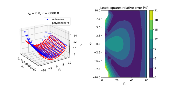
Figure 4: Left: least-squares fit of $f_{1}$ samples (blue dots) by the polynomial model (red curve) given $i_{w}$ and $T$. Right: contour plot of the percent relative fitting error.

The residue of $y^{\top}(Q-R-P)y=0$ illustrates the accuracy of the DC decomposition of the polynomial approximation, and is excellent in both cases.

Finally, we verify that there was no convexity violation by computing the Hessians of the functions at each test point and checking for positive semidefiniteness. A typical DC decomposition is shown in Figure 5 (with projection).

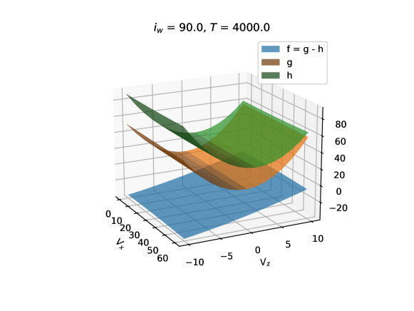
Figure 5: DC decomposition $f=g-h$ for given $i_{w}$ and $T$.

4.2 Forward transition

At first, we set the penalty matrix in the objective to $Q_{x}=\text{diag}(1,1\mathrm{e}{+4})$ to achieve a constant altitude forward transition. The results are shown in Figure 6. As the aircraft transitions from powered lift to cruise, the velocity magnitude increases, the thrust and tiltwing angle decrease, illustrating the change in lift generation from propellers to wing. The tiltwing angle drop at the beginning results in an increase in the effective angle of attack. Note that the solution (plain blue) has converged to the desired reference trajectory (dashed green) despite the initial discrepancy with the feasible guess trajectory (dashed orange).

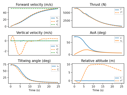
Figure 6: Constant altitude forward transition.

The objective can be changed to achieve faster transitions. For example, if the penalty matrix is set to $Q_{x}=\text{diag}(100,1)$, the obtained results are presented in Figure 7. The reference forward velocity is achieved faster than previously, but this comes at the expense of an altitude drops. A trade-off between both objectives (reaching the desired forward or vertical velocity) can be achieved by varying the penalty matrix.

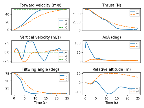
Figure 7: A faster forward transition.

4.3 Backward transition

For completeness, we consider the scenario consisting of a backward transition with an increase in altitude, see Figure 8. This is characterised by a decrease in velocity magnitude and increase in thrust to support the powered flight mode (hover). An increase in altitude of about 75 m is needed for this manoeuvre, and the wing is stalled.

Figure 8: Backward transition.

4.4 Robustness to wind

To simulate the effect of wind gust on the aircraft, we consider EASA "Means of Compliance with the Special Condition VTOL", §2215 on flight load conditions [16] and assume that the aircraft is subject to a discrete wind gust with velocity $U$ following a "one-minus-cosine" law

$$U(x_{g})=\frac{U_{de}}{2}\left(1-\cos{\left(\frac{2\pi x_{g}}{25\bar{c}}\right)}\right),$$

where $0\leq x_{g}\leq 25\bar{c}$ is the distance penetrated into the gust, $\bar{c}$ is the mean geometric chord of the wing, and $U_{de}$ the design gust velocity. The wind gust parameters are reported in Table 4 and the gust velocity profile with these values is presented in Figure 9.

We then consider both crosswind and headwind scenarios for the gust direction.

4.4.1 Crosswind

It is assumed that the wind gust velocity acts normally to the aircraft flight path (velocity vector), i.e. along $\vec{L}$ in Figure 1. This has the effect of modifying the velocity and angle of attack seen by the wing and hence the lift and drag as follows

$$L=\tfrac{1}{2}\lambda\rho SC_{L}(\alpha_{e}^{\prime})V_{e}^{\prime 2}+\tfrac{1}{2}(1-\lambda)\rho SC_{L}(\alpha^{\prime})V^{\prime 2},$$

$$D=\tfrac{1}{2}\lambda\rho SC_{D}(\alpha_{e}^{\prime})V_{e}^{\prime 2}+\tfrac{1}{2}(1-\lambda)\rho SC_{D}(\alpha^{\prime})V^{\prime 2},$$

where

$$V^{\prime 2}={V^{2}+U(x_{g})^{2}},\quad\alpha^{\prime}=\alpha+\arctan{\left(\frac{U}{V}\right)},$$

$$V_{e}^{\prime 2}={V_{e}^{2}+U(x_{g})^{2}},\quad\alpha_{e}^{\prime}=\alpha_{e}+\arctan{\left(\frac{U}{V_{e}}\right)}.$$

The torque created by the imbalance in lift due to the depth difference along the wing is assumed to be negligible, which justifies our assumption that no wind gust disturbance acts on the tiltwing rotational dynamics in equation (4).

To evaluate the time varying wind gust bounds $[\underline{W}_{i}(t),\overline{W}_{i}(t)]$, $\forall i\in\{x,z\}$ we consider the maximum increment in drag and lift along the guess trajectory as follows

$$\Delta L_{\text{max}}(t)=\tfrac{1}{2}\rho SC_{L}(\alpha^{\circ})U_{de}^{2}+\tfrac{1}{2}\rho Sb_{1}\arctan{(U_{de}/V^{\circ})}(U_{de}^{2}+V^{\circ^{2}})$$

$$\Delta D_{\text{max}}(t)=\tfrac{1}{2}\rho SC_{D}(\alpha^{\circ})U_{de}^{2}+\tfrac{1}{2}\rho S(a_{2}(\arctan{(U_{de}/V^{\circ})}^{2}+2\alpha^{\circ}\arctan{(U_{de}/V^{\circ})})+a_{1}\arctan{(U_{de}/V^{\circ})})(U_{de}^{2}+V^{\circ^{2}}).$$

Parameter	Symbol	Value	Units
Design gust velocity	$U_{de}$	$9.14$	$\mathrm{m}\mathrm{/}\mathrm{s}$
Mean geometric chord	$\bar{c}$	$1$	$\mathrm{m}$

Table 4: Wind gust parameters as defined in [16].

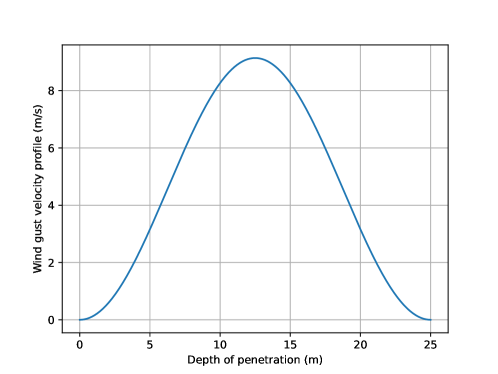
Figure 9: Wind gust velocity profile.

In order to evaluate the effect of wind gusts on the aircraft, we conduct multiple simulations by varying the instant at which the aircraft encounters a wind gust during the forward and backward transitions and we observe the subsequent deviations from the reference:

• Forward transition with crosswind. The results are illustrated in Figure 10. For the wind gusts occuring at times $t=5$ $\mathrm{s}$ and $t=10$ $\mathrm{s}$, the deviations observed are reasonable with vertical velocity not exceeding $3$ $\mathrm{m}\mathrm{/}\mathrm{s}$ in magnitude. The deviation is more important when the disturbance occurs at $t=0$ $\mathrm{s}$ since the vehicle is in hover mode, but the system eventually recovers and stabilises.

• Backward transition with crosswind. The backward transition could not be achieved with crosswind gusts of $9.14m/s$, so the wind speed was reduced to $5.14m/s$ to obtain the results in Figure 12. In all cases, the forward and vertical velocities are slightly perturbed and the system eventually recovers.

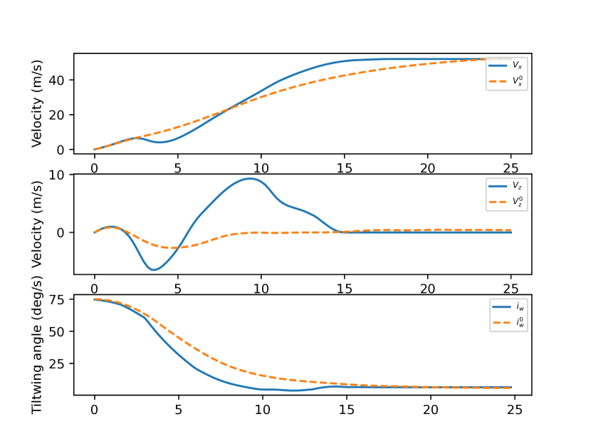
(a) $t=0s$

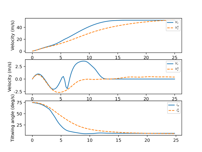
(b) $t=5s$

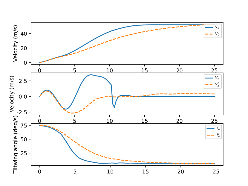
(c) $t=10s$

Figure 10: Forward transition with crosswind gust occurring at various times.

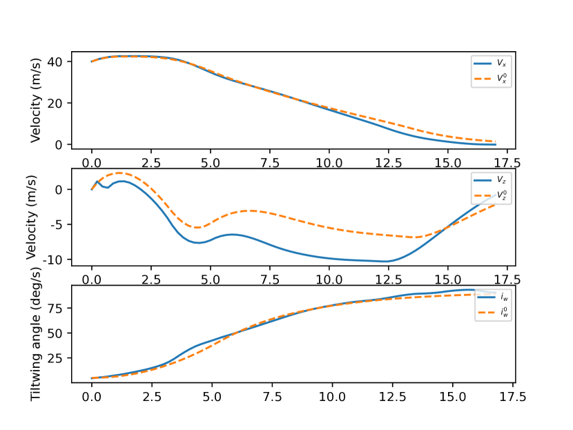
(a) $t=0s$

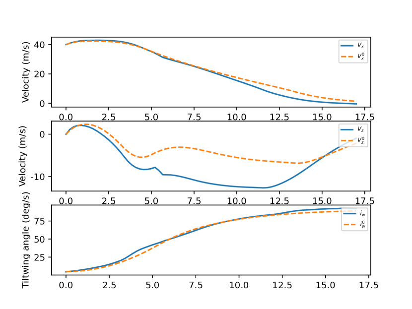
(b) $t=5s$

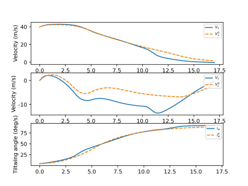
(c) $t=10s$

Figure 11: Backward transition with crosswind gust occurring at various times.

4.4.2 Headwind

In case of headwind, the wind gust velocity acts anti-parallel to the aircraft velocity vector $\vec{V}$. This modifies the lift and drag as follows (note that this does not affect the angle of attack)

$$L=\tfrac{1}{2}\lambda\rho SC_{L}(\alpha_{e})V_{e}^{\prime 2}+\tfrac{1}{2}(1-\lambda)\rho SC_{L}(\alpha)V^{\prime 2},$$

$$D=\tfrac{1}{2}\lambda\rho SC_{D}(\alpha_{e}^{\prime})V_{e}^{\prime 2}+\tfrac{1}{2}(1-\lambda)\rho SC_{D}(\alpha^{\prime})V^{\prime 2},$$

where

$$V^{\prime 2}={V^{2}+U(x_{g})^{2}},$$

$$V_{e}^{\prime 2}={V_{e}^{2}+U(x_{g})^{2}},$$

and we deduce the maximum increment in drag and lift along the guess trajectory as follows

$$\Delta L_{\text{max}}(t)=\tfrac{1}{2}\rho SC_{L}(\alpha^{\circ})U_{de}^{2}$$

$$\Delta D_{\text{max}}(t)=\tfrac{1}{2}\rho SC_{D}(\alpha^{\circ})U_{de}^{2}.$$

We then conduct a series of simulations of both forward and backward transitions subject to headwind gusts occurring at various time instants:

• Forward transition with headwind. The results are presented in Figure 12. As illustrated, there is almost no variation depending on when the gust is applied on the aircraft, which seems to indicate that headwinds are much less harmful than crosswinds for the closed-loop stability. This is due to the angle of attack not being affected by headwinds.

• Backward transition with headwind. The results are presented in Figure 13. Note that contrary to the simulations with crosswinds, the aircraft is capable to withstand headwinds at $9.14m/s$.

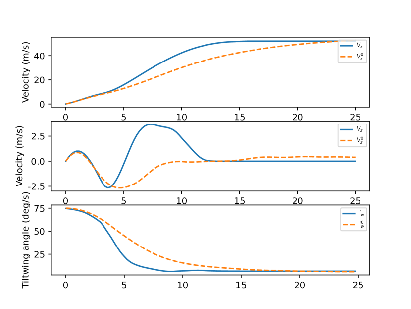
(a) $t=0s$

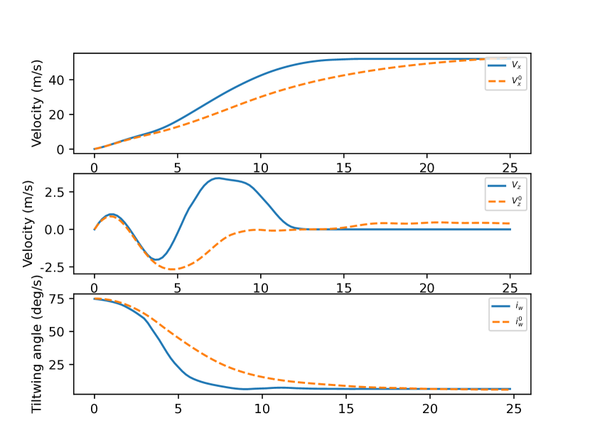
(b) $t=5s$

(c) $t=10s$

Figure 12: Forward transition with headwind gust occurring at various times.

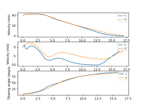
Figure 13: Backward transition with headwind gust.

4.5 Convergence

Convergence of the algorithm is illustrated in Figure 14, showing that the objective value decreases at each time step. Finally, Figure 15 shows the average computation time to solve problem $\mathcal{P}$ as a function of the number of discretisation points $N$. The experiment was conducted on a MacBook Pro with a 2.9 GHz dual-core Intel Core i7 processor (mid-2012). For example, for $N=100$, the average computation time was $1.9s$. Although this would not allow to compute the solution within the specified time step in real time, it should be noted that CVXPY is not optimised for performance and that reductions in computation times of about an order of magnitude can be expected with first order solvers such as ADMM [17]. This is in stark contrast to state-of-the-art generic NLP approaches that quote computation times of the order of minutes to solve similar VTOL transition optimisation problems (e.g. see [12]).

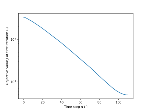
Figure 14: Objective at each time step.

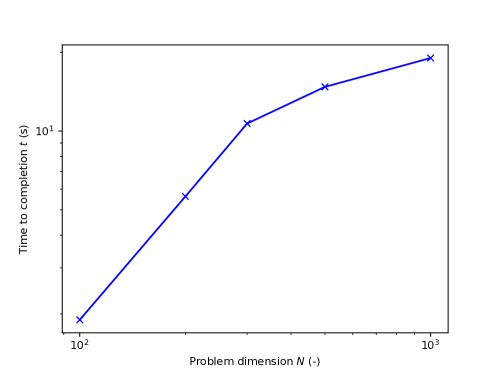
Figure 15: Time to completion as a function of problem dimension.

5 Conclusion

We presented a novel computationally tractable robust data-driven tube MPC scheme based on a DC decomposition of the nonlinear dynamics of a tiltwing VTOL aircraft to achieve robust transitions in the presence of wind. The DC structure of the dynamics allowed us to express the MPC optimisation at each time step as a sequence of convex programs generated by successively linearising around guess trajectories and bounding tightly the effect of the necessarily convex linearisation errors. We demonstrated the viability of the scheme by considering a case study inspired from the Airbus Vahana $A^{3}$ VTOL aircraft using a mixture of data-based and mathematical models. Forward and backward transitions were successfully achieved, as well as transitions subject to wind gusts. Future work has been identified as follows: i) leveraging first order solvers (e.g. ADMM) to accelerate computation times and enable real-time implementations; ii) complete study of the effect of: uncertainty set parameterisation, DC decomposition technique, approximation function, etc. on the performances of the algorithm; iii) adaptation of the method to function approximation via deep neural network to allow a higher degree of generalisability ; iv) extension of the framework to constraints of stochastic nature (e.g. von Kármán wind turbulence model could be leveraged to achieve VTOL transitions that are less conservative).

References

- McKinsey [2021] McKinsey, “Study on the societal acceptance of Urban Air Mobility in Europe,” European Union Aviation Safety Agency (EASA), 2021.
- Kadhiresan and Duffy [2019] Kadhiresan, A. R., and Duffy, M. J., “Conceptual design and mission analysis for eVTOL urban air mobility flight vehicle configurations,” AIAA aviation 2019 forum, 2019, p. 2873.
- Saias et al. [2022] Saias, C. A., Roumeliotis, I., Goulos, I., Pachidis, V., and Bacic, M., “Assessment of hydrogen fuel for rotorcraft applications,” International Journal of Hydrogen Energy, Vol. 47, No. 76, 2022, pp. 32655–32668. https://doi.org/10.1016/j.ijhydene.2022.06.316, URL https://www.sciencedirect.com/science/article/pii/S0360319922030099.
- Kouvaritakis and Cannon [2016] Kouvaritakis, B., and Cannon, M., “Model predictive control,” Switzerland: Springer International Publishing, Vol. 38, 2016.
- Chiappinelli et al. [2019] Chiappinelli, R., Cohen, M., Doff-Sotta, M., Nahon, M., Forbes, J. R., and Apkarian, J., “Modeling and control of a passively-coupled tilt-rotor vertical takeoff and landing aircraft,” 2019 International Conference on Robotics and Automation (ICRA), IEEE, 2019, pp. 4141–4147.
- Rohr et al. [2019] Rohr, D., Stastny, T., Verling, S., and Siegwart, R., “Attitude and Cruise Control of a VTOL Tiltwing UAV,” IEEE Robotics and Automation Letters, Vol. 4, No. 3, 2019, pp. 2683–2690.
- Sobiesiak et al. [2019] Sobiesiak, L., Fortier-Topping, H., Beaudette, D., Bolduc-Teasdale, F., de Lafontaine, J., Nagaty, A., Neveu, D., and Rancourt, D., “Modelling and control of transition flight of an eVTOL tandem tilt-wing aircraft,” 2019 8th European conference for aeronautics and aerospace sciences (EUCASS), 2019, pp. 1–14.
- Doff-Sotta and Cannon [2022] Doff-Sotta, M., and Cannon, M., “Difference of convex functions in robust tube nonlinear MPC,” 2022 Conference on Decision and Control (CDC), IEEE, 2022, pp. 3044–3050.
- Ahmadi and Hall [2018] Ahmadi, A. A., and Hall, G., “DC decomposition of nonconvex polynomials with algebraic techniques,” Mathematical Programming, Vol. 169, No. 1, 2018, pp. 69–94.
- Doff-Sotta et al. [2022] Doff-Sotta, M., Cannon, M., and Bacic, M., “Fast optimal trajectory generation for a tiltwing VTOL aircraft with application to urban air mobility,” 2022 American Control Conference (ACC), IEEE, 2022, pp. 4036–4041.
- Doff-Sotta et al. [2023] Doff-Sotta, M., Cannon, M., and Bacic, M., “Robust trajectory optimisation for transitions of tiltwing VTOL aircraft,” arXiv preprint arXiv:2302.04361, 2023.
- Chauhan and Martins [2019] Chauhan, S. S., and Martins, J. R., “Tilt-wing eVTOL takeoff trajectory optimization,” Journal of Aircraft, 2019, pp. 1–20.
- Hartman [1959] Hartman, P., “On functions representable as a difference of convex functions.” Pacific Journal of Mathematics, Vol. 9, No. 3, 1959, pp. 707–713.
- Diamond and Boyd [2016] Diamond, S., and Boyd, S., “CVXPY: A Python-embedded modeling language for convex optimization,” Journal of Machine Learning Research, Vol. 17, No. 83, 2016, pp. 1–5.
- ApS [2021] ApS, M., Introducing the MOSEK Optimization Suite 9.3.6, 2021.
- EASA [2021] EASA, “Means of Compliance with the Special Condition VTOL,” European Union Aviation Safety Agency, 2021.
- Doff-Sotta et al. [2021] Doff-Sotta, M., Cannon, M., and Bacic, M., “Predictive energy management for hybrid electric aircraft propulsion systems,” IEEE Transactions on Control Systems Technology, 2021.