Estimation of Complex-Valued Laplacian Matrices for Topology Identification in Power Systems

Abstract

In this paper, we investigate the problem of estimating a complex-valued Laplacian matrix from a linear Gaussian model, with a focus on its application in the estimation of admittance matrices in power systems. The proposed approach is based on a constrained maximum likelihood estimator (CMLE) of the complex-valued Laplacian, which is formulated as an optimization problem with Laplacian and sparsity constraints. The complex-valued Laplacian is a symmetric, non-Hermitian matrix that exhibits a joint sparsity pattern between its real and imaginary parts. Leveraging the $\ell_{1}$ relaxation and the joint sparsity, we develop two estimation algorithms for the implementation of the CMLE. The first algorithm is based on casting the optimization problem as a semi-definite programming (SDP) problem, while the second algorithm is based on developing an efficient augmented Lagrangian method (ALM) solution. Next, we apply the proposed SDP and ALM algorithms for the problem of estimating the admittance matrix under three commonly-used measurement models, that stem from Kirchhoff’s and Ohm’s laws, each with different assumptions and simplifications: 1) the nonlinear alternating current (AC) model; 2) the decoupled linear power flow (DLPF) model; and 3) the direct current (DC) model. The performance of the SDP and the ALM algorithms is evaluated using data from the IEEE $33$-bus power system data under different settings. The numerical experiments demonstrate that the proposed algorithms outperform existing methods in terms of mean-squared-error (MSE) and F-score, thus, providing a more accurate recovery of the admittance matrix.

I Introduction

The Laplacian matrix is a critical tool for studying the properties of graphs and is central to many key concepts in graph signal processing (GSP), machine learning, and networked data analysis. Examples include semi-supervised learning, dimensionality reduction, community detection in complex networks, spectral clustering, and solving partial differential equations on graphs. It can also be used to define notions of smoothness and regularity on graphs, making it a powerful tool for analyzing and understanding the structure of complex data [2, 3, 4]. Thus, the estimation of the Laplacian matrix is a fundamental task in various fields.

Complex-valued graph signals arise in several real-world applications [5], such as multi-agent systems [6], wireless communication systems [7], voltage and power phasors in electrical networks [8, 9, 10], and probabilistic graphical models with complex-valued multivariate Gaussian vectors [11]. Despite the widespread use of complex-valued graph signals, the recovery of complex-valued Laplacians is a crucial problem that has not been well explored.

Numerous approaches have been proposed in the literature for the estimation of the real-valued Laplacian matrix. Notably, the seminal work in [12] introduced a regularization framework for sparse precision (inverse covariance) estimation in graphical models, giving rise to the graphical Lasso algorithm. Subsequently, researchers have explored various computationally efficient variations and extensions of graphical Lasso in recent years (see, e.g., [13, 14]). In particular, graphical Lasso has recently been developed for proper and improper complex Gaussian graphical models in [11]. Lately, there has been growing interest in developing estimation methods for cases where the precision matrix is a Laplacian matrix [15, 16, 17]. The problem of learning the graph Laplacian from smooth graph signals has been considered in [18, 19, 20]. However, these methods were developed for real-valued Laplacian matrices and for graphical models, whereas our focus lies in the estimation of a complex-valued Laplacian matrix in a physical linear-Gaussian model, where the Laplacian matrix appears in the expectation. This presents challenges, as the complex-valued Laplacian matrix is symmetric but not Hermitian, and exhibits a joint sparsity [21, 22] pattern between its real and imaginary parts. Additionally, the solution of complex-valued optimization problems by using real-valued methods may be time-consuming and difficult, especially in the presence of complicated constraints [23], such as joint sparsity.

Admittance matrix estimation in power systems is a particular example of complex-valued estimation, and is the main motivation for this work. The modern electric grid is one of the largest and most complex cyber-physical systems today, where a power system can be represented as an undirected weighted graph with grid buses as nodes (vertices) and transmission lines as edges. Topology information plays a critical role in various aspects of modern power systems, including analysis, security, control, and stability assessment of power systems [24, 25, 26, 27]. Gaining knowledge of grid topology, summarized in the admittance matrix, is essential for effective grid optimization and monitoring tasks. However, obtaining real-time information about topology and line parameters might be challenging, especially in distribution networks. Hence, accurate topology identification and precise line-parameter estimation become crucial for ensuring the efficiency and reliability of the network operations. Additionally, topology identification achieved through admittance matrix estimation can serve as a valuable tool for event detection, such as identifying faults and line outages [28], and detection of potential cyberattacks [9, 29]. Furthermore, with the increasing integration of distributed renewable energy resources, the importance of admittance matrix estimation has risen significantly, making it an indispensable element in addressing the challenges of modern power systems.

Different approaches have been proposed for learning the topology of electrical networks. Graph theory and graphical models have been utilized in power systems for various tasks (see, e.g,. [30, 31, 32]). In particular, topology identification and the estimation of the topologies of distribution grids have been discussed in [33, 34, 35, 36, 37, 38]. Other works explored the detection of topological changes and the identification of edge disconnections in electrical networks using hypothesis testing methods (see [39, 40] and [41, 42], respectively). The methods in [43, 44, 45, 46] can reveal part of the grid information, such as the grid connectivity and the eigenvectors of the topology matrix. Blind estimation of states and the real-valued admittance (susceptance) matrix has been studied in [35]. Additionally, in [38], a novel algorithm based on the recursive grouping algorithm [47], is suggested for learning the distribution grid topology and estimating transmission line impedances. However, these methods estimate the real-valued admittance matrix and are often based on linearized power flow models (e.g. a direct current (DC) model), or on restrictive assumptions on the network structure (e.g., a tree graph). Other methods rely on data-driven approaches using historical measurements. However, these approaches demand large amounts of data, which is unavailable in current systems. A nonlinear weighted least-square error algorithm is used to estimate line parameters in [48], while a total least-squares method is applied in [49]; however, total least-squares method becomes unstable at low signal-to-noise ratio (SNR) values due to significant errors in power measurements. To conclude, existing methods do not estimate the full complex-valued admittance matrix under Laplacian constraints using the full nonlinear alternating current (AC) model.

In this paper, we address the problem of estimating a complex-valued Laplacian matrix from linear Gaussian models. The complex-valued Laplacian is a symmetric but non-Hermitian matrix, exhibiting almost joint sparsity patterns between its real and imaginary parts. The joint sparsity property is experimentally validated in this paper for the admittance matrix in electrical network applications. This property necessitates the development of a unified algorithm capable of simultaneously estimating the two real-valued, sparse, Laplacian matrices under the joint-sparsity constraint. To recover the complex-valued Laplacian matrix, we propose a constrained maximum likelihood estimator (CMLE) formulated as an optimization problem for a general objective function with graph Laplacian and joint-sparsity constraints. To efficiently solve for the CMLE, we develop two approaches: the first uses a semi-definite programming (SDP) formulation and the second employs the augmented Lagrangian method (ALM) [50]. In the second part of this paper, we model the power network as a graph and describe the sparsity and Laplacian constraints of the admittance matrix. We then apply the proposed estimation methods to three commonly-used power-flow measurement models: the nonlinear AC model, the extended linear decoupled linear power flow (DLPF) model, and the linear DC model, each with different assumptions and simplifications. We evaluate the performance of the proposed algorithms on IEEE 33-bus power system data under various settings and SNR values. Numerical experiments demonstrate that the proposed algorithms outperform existing methods in terms of mean-squared-error (MSE) and F-score, leading to more accurate recovery of the admittance matrix.

Notation and Organization: In this paper, vectors are denoted by boldface lowercase letters and matrices by boldface uppercase letters. The $K\times K$ identity matrix is denoted by ${\bf{I}}_{K}$, and ${\bf{1}}$ and ${\bf{0}}$ denote the vectors of ones and zeros, respectively. The notation $|\cdot|$ and $\otimes$ denote the determinant operator and the Kronecker product, respectively. For any vector ${\bf{u}}$, $\|{\bf{u}}\|_{2}$ denotes the Euclidean-norm. For any matrix ${\bf{A}}$, ${\bf{A}}\succeq{\bf{0}}$ means that ${\bf{A}}$ is a positive semi-definite matrix, and ${\bf{A}}^{-1}$ and $\|{\bf{A}}\|_{F}$ are its inverse and Frobenius norm, respectively, $\|{\bf{A}}\|_{1,{\text{off}}}$ is the sum of the absolute values of all off-diagonal elements of ${\bf{A}}$, and ${\text{vec}}({\bf{A}})$ is the vector obtained by stacking the columns of ${\bf{A}}$ with ${\text{unvec}}({\text{vec}}({\bf{A}}))={\bf{A}}$. For a vector ${\bf{a}}$, ${\text{diag}}({\bf{a}})$ is a diagonal matrix whose $n$th diagonal entry is $a_{n}$; when applied to a matrix, ${\text{diag}}({\bf{A}})$ is a vector with the diagonal elements of ${\bf{A}}$. In addition, ${\text{ddiag}}({\bf{A}})={\text{diag}}({\text{diag}}({\bf{A}}))$. We also have $x^{+}=\max\{x,0\}$. We denote by ${\bf{a}}^{i}$ the $i$th row of the matrix ${\bf{A}}$. The $(p,r)$-norm of a matrix ${\bf{A}}$ is defined as

$$||{\bf{A}}||_{p,r}=\left(\sum\nolimits_{i=1}^{M}||{\bf{a}}^{i}||_{p}^{r}\right)^{\frac{1}{r}}.$$ (1)

The gradient of a scalar function $f({\bf{x}})$ w.r.t. the vector ${\bf{x}}$ is a column vector with the dimensions of ${\bf{x}}$.

The rest of this paper is organized as follows. In Section II, we describe the considered complex-valued Laplacian matrix estimation model, and discuss the properties of the resulting optimization problem. In Section III, we develop the SDP and ALM algorithms to solve this optimization. In Section IV, we implement the proposed algorithms for the three power system models. Subsequently, simulations are shown in Section V. Finally, the paper is concluded in Section VI.

II Complex-valued Laplacian estimation

In this section, we formulate the problem of estimating a complex-valued Laplacian matrix within general statistical models. Since the primary focus of this paper lies in the application of admittance matrix identification in electrical networks, we derive the properties of the complex-valued Laplacian for linear quadratic models, as in electrical network theory. In particular, in Subsection II-A, we represent the power network as a graph and describe the constraints imposed by the complex-valued Laplacian structure. In Subsection II-B, we experimentally validate the joint sparsity property of the complex-valued admittance matrix. Then, we formulate the constrained estimation problem of the complex-valued Laplacian for a general objective function in Subsection II-C, with an emphasis on the crucial constraint of joint sparsity between the real and imaginary parts of the Laplacian.

II-A Model and problem formulation

A power system can be represented as an undirected connected weighted graph, ${\pazocal{G}}({\pazocal{V}},\xi)$, where the set of vertices, ${\pazocal{V}}=\{1,\ldots,M\}$, comprises the buses (generators/loads) and the set of edges, $\xi$, comprises the transmission lines. The edge $(m,k)\in\xi$ corresponds to the transmission line between buses $m$ and $k$, and is characterized by the line admittance, $y_{m,k}\in{\mathbb{C}}$. The system (nodal) admittance matrix is a $M\times M$ complex symmetric matrix, where its $(m,k)-th$ element is given by (p. 97 in [51])

$$[{\bf{Y}}]_{m,k}=\begin{cases}\displaystyle-\sum_{n\in{\mathcal{N}}_{m}}y_{m,n},&m=k\\ \displaystyle y_{m,k},&m\neq k\\ \displaystyle 0&\text{otherwise}\end{cases},$$ (2)

where $m,k=1,\ldots,M$. In this graph representation, ${\bf{Y}}$ is a complex-valued Laplacian matrix.

The admittance matrix from (2) can be decomposed as

$${\bf{Y}}={\bf{G}}+j{\bf{B}},$$ (3)

where the conductance matrix, ${\bf{G}}\in{\mathbb{R}}^{M\times M}$, and the minus susceptance matrix, $\tilde{{\bf{B}}}\stackrel{{\scriptstyle\triangle}}{{=}}-{\bf{B}}\in{\mathbb{R}}^{M\times M}$, are both real-valued Laplacian matrices. That is, $\tilde{{\bf{B}}}$ and ${\bf{G}}$ belong to the set

$$\mathcal{L}=\{{\bf{L}}\in\mathcal{S}^{M}_{+}|[{\bf{L}}]_{m,k}\leq 0,~{}\forall m\neq k,\quad{\bf{L}}{\bf{1}}={\bf{0}}\},$$ (4)

where $\mathcal{S}^{M}_{+}$ is the set of real, symmetric, positive semi-definite matrices. As a result, it can be seen that ${\bf{Y}}$ is a symmetric but non-Hermitian matrix. Thus, its eigenvalues may not be real, and its eigenvectors may not be orthogonal [52]. For the sake of simplicity of computation, in this paper, we estimate the matrices ${\bf{G}}$ and $\tilde{{\bf{B}}}$, which are real-valued Laplacian matrices.

Numerous Laplacian learning algorithms are based on the assumption that the Laplacian matrix is a sparse matrix. In addition, for the considered application, electrical networks are known to be sparse, since the buses are usually only connected to 2-5 neighbors [53]. Therefore, we assume here that matrices ${\bf{G}}$ and $\tilde{{\bf{B}}}$ are sparse. Previous works have often assumed that the support sets of these sparse matrices are either independent (where each matrix is estimated separately and in parallel), or identical [1]. However, in practical scenarios, it is more realistic to assume that the matrices do not share the exact same support, but have similar support sets, as they represent different aspects of the network. In particular, in Subsection II-B, we validate this property for the admittance matrix. This necessitates the development of a unified algorithm capable of simultaneously estimating the two real-valued, sparse, Laplacian matrices under the joint-sparsity constraint [21, 22].

To conclude, the real and imaginary parts of the complex-valued Laplacian matrix, ${\bf{G}}$ and $\tilde{{\bf{B}}}$, belong to $\mathcal{L}$ in (4) and are jointly sparse. Thus, they have the following properties:

1. Symmetry: ${\bf{G}}={\bf{G}}^{T}$, $\tilde{{\bf{B}}}=\tilde{{\bf{B}}}^{T}$

2. Null-space property: ${\bf{G}}{\bf{1}}={\bf{0}}$, $\tilde{{\bf{B}}}{\bf{1}}={\bf{0}}$

3. Non-positive off-diagonal entries: $[{\bf{G}}]_{m,k}\leq 0$,
   $[\tilde{{\bf{B}}}]_{m,k}\leq 0$, $\forall m,k=1,\dots,M$, $m\neq k$

4. Positive semi-definiteness: ${\bf{G}}\succeq{\bf{0}}$, $\tilde{{\bf{B}}}\succeq{\bf{0}}$

5. ${\bf{G}}$ and $\tilde{{\bf{B}}}$ are almost jointly-sparse matrices.

II-B Experimental validation: the joint sparsity of the admittance matrix in typical networks

For the purpose of experimental validation of the sparsity patterns of $\tilde{{\bf{B}}}$ and ${\bf{G}}$ in typical electrical networks, in Table I we present the size of the support of the two Laplacian matrices (i.e. the connectivity pattern of the graph based on ${\bf{G}}$ and $\tilde{{\bf{B}}}$) for the IEEE test cases [54]. In addition, we compute the F-score between the two matrices [55] (which measures the differences in the sparsity patterns of $\tilde{\bf{B}}$ and ${\bf{G}}$), by treating one of the matrices ($\tilde{\bf{B}}$ or ${\bf{G}}$) as the ground truth and the other as the estimate. This F-score takes values between $0$ and $1$, where, in this case, $1$ indicates a situation where the supports of $\tilde{{\bf{B}}}$ and of ${\bf{G}}$ are identical. It can be seen from this table that the matrices are almost (but not perfectly) jointly sparse. This assumption is more restrictive than assuming that each matrix is sparse with its own independent support. From the evaluation of the ratio between the matrix elements, it can also be seen that the magnitudes of the elements in ${\bf{B}}$ are larger than the magnitudes of the elements in ${\bf{G}}$. Finally, in Fig. 1(b), we illustrate the relations between the real and imaginary parts of the admittance matrix, ${\bf{G}}$ and $\tilde{{\bf{B}}}$, of the IEEE 14-bus system. This figure shows that the supports of the two matrices are sparse, with similar but not identical patterns.

	IEEE test case system
Measures	14-bus	33-bus	57-bus	118-bus	145-bus
$|\xi_{\bf{G}}|$	15	32	62	170	409
$|\xi_{\bf{B}}|$	20	32	78	179	422
F-score	0.875	1	0.9160	0.9807	0.9836
Ratio	2.683	0.853	2.785	5.396	14.180

TABLE I: Properties of IEEE test case systems: the first and second rows display the number of edges (i.e. number of nonzeros in their lower triangular) in matrices ${\bf{G}}$ and ${\bf{B}}$, respectively. The third row is the F-score between the two matrices, which measures the differences in the sparsity patterns of ${\bf{B}}$ and ${\bf{G}}$. Finally, the fourth row is the average ratio of magnitude between two elements in the matrices, $\frac{1}{M^{2}}\sum_{m=1}^{M}\sum_{k=1}^{M}\frac{[{\bf{B}}]_{k,m}}{[{\bf{G}}]_{k,m}}$.

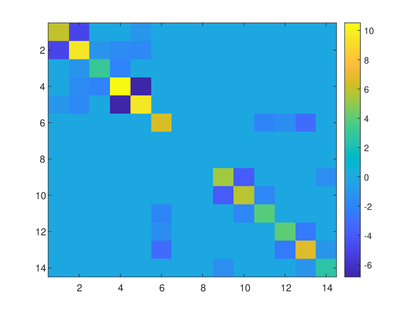
(a)

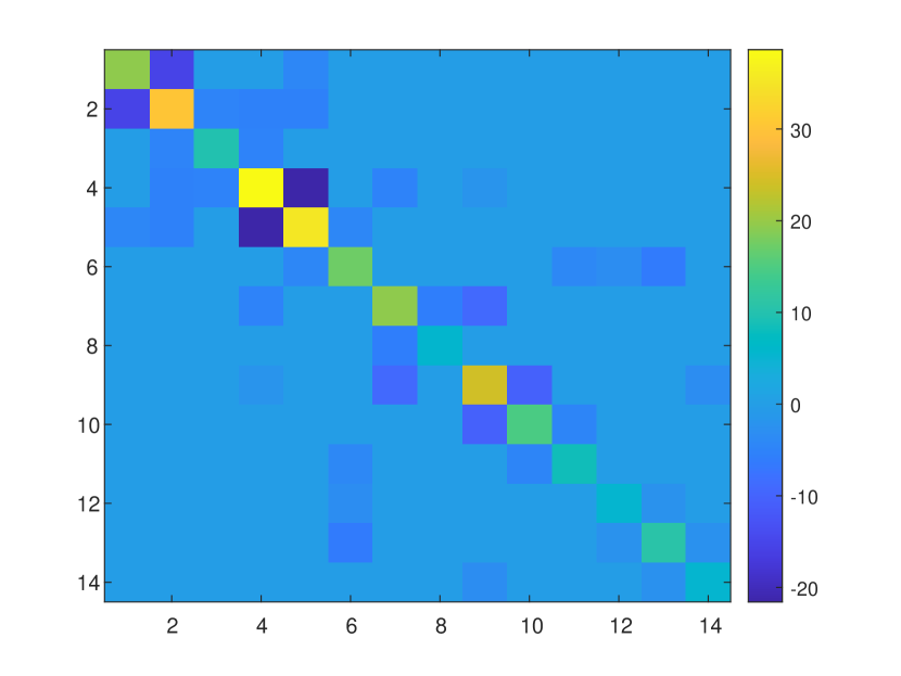
(b)

Figure 1: Illustration of the real (a) and imaginary (b) parts of the admittance matrix for IEEE 14-bus system.

II-C CMLE

The CMLE is a variant of the maximum likelihood estimator (MLE) that is used when there are parametric constraints on the unknown parameters to be estimated, and has appealing asymptotic performance [56, 57]. In this work, given a measurement model with the general log-likelihood $-\psi({\bf{X}};{\bf{G}},\tilde{{\bf{B}}})$, our goal is to estimate ${\bf{G}}$ and $\tilde{{\bf{B}}}$ from the data, ${\bf{X}}$. The parametric constraints described by properties P.1-P.5 of the Laplacian matrices ${\bf{G}}$ and $\tilde{{\bf{B}}}$ imply that the CMLE of ${\bf{G}}$ and $\tilde{{\bf{B}}}$ can be written as the following optimization problem:

$$\min_{{\bf{G}},\tilde{{\bf{B}}}\in\mathbb{R}^{M\times M}}\psi({\bf{X}};{\bf{G}},\tilde{{\bf{B}}})$$ (5)

s.t. $${\text{C.1}})~{}{\bf{G}}={\bf{G}}^{T},~{}\tilde{{\bf{B}}}=\tilde{{\bf{B}}}^{T}$$

$${\text{C.2}})~{}{\bf{G}}{\bf{1}}={\bf{0}},~{}\tilde{{\bf{B}}}{\bf{1}}={\bf{0}}$$

$${\text{C.3}})~{}[{\bf{G}}]_{m,k}\leq 0,~{}[\tilde{{\bf{B}}}]_{m,k}\leq 0,~{}\forall m\neq k,k=1,\dots,M$$

$${\text{C.4}})~{}{\bf{G}}\succeq{\bf{0}},~{}\tilde{{\bf{B}}}\succeq{\bf{0}}$$

$${\text{C.5}})~{}{\bf{G}},~{}\tilde{{\bf{B}}}{\text{ are almost jointly-sparse matrices}}.$$

The estimation of the complex-valued Laplacian matrix in different applications involves the utilization of different measurement models. These models are functions of the network topology (${\bf{G}}$ and $\tilde{{\bf{B}}}$), the available measurements or given data (${\bf{X}}$), and may also incorporate additional noise and errors. The specific log-likelihood of the measurement model, $-\psi({\bf{X}},{\bf{G}},{\bf{B}})$, serves as the objective function in our optimization problem, as presented in (5). Notably, the constraints are identical across all models. This section provides a general overview of the problem, while a discussion of specific objective functions associated with different measurement models in power system applications is presented in Section IV.

In order to solve (5), we first note that Constraint C.5 in (5) can be mathematically formulated as[22]:

$${\text{C.5}})~{}\left\|[\text{Vec}_{\ell}({\bf{G}}),\text{Vec}_{\ell}(\tilde{{\bf{B}}})]\right\|_{p,0}\leq s,$$ (6)

where $s$ is a sparsity level. The $(p,0)$-norm of a matrix is obtained from the definition in (1) with $r=0$. This norm counts the number of rows in its matrix argument that contain nonzero entries, and hence enforces row-sparsity [22, 58]. Thus, in our case, the constraint of the joint sparsity assumption implies that the matrix $[{\text{Vec}}_{\ell}({\bf{G}}),{\text{Vec}}_{\ell}(\tilde{{\bf{B}}})]$ is a row-sparse matrix, i.e. there are many zero elements shared jointly by the two matrices ${\bf{G}}$ and $\tilde{{\bf{B}}}$. It is worth noting that the operator $\text{Vec}_{\ell}$ only returns the off-diagonal elements of its matrix argument. As a result, the zero semi-norm constraint in (6) is only applied on the off-diagonal elements of the matrices, where the diagonal elements are known to be nonzero.

Now, it is known that symmetric, diagonally-dominant matrices with real nonnegative diagonal entries, such as ${\bf{G}}$ and $\tilde{{\bf{B}}}$ under Constraints C.1-C.3, are necessarily positive semi-definite matrices (see, e.g., p. 392 in [52]). Consequently, Constraint C.4 is redundant and can be eliminated without affecting the solution of (5)-(6). In addition, Constraint C.5, which enforces sparsity in the matrices, renders the optimization problem in (6) non-convex. However, this sparsity constraint can be approximated by introducing an $\ell_{1}$-regularization [59], thereby transforming the problem in (5) into an approximate convex optimization problem. As a result, we can remove both constraints C.4 and C.5, and modify the objective function in (6) to obtain the following regularized convex optimization problem:

$$\min_{{\bf{G}},\tilde{{\bf{B}}}\in\mathbb{R}^{M\times M}}\psi({\bf{X}},{\bf{G}},\tilde{{\bf{B}}})\hskip 99.58464pt$$

$$+\lambda\left\|[w_{G}\text{Vec}_{\ell}({\bf{G}}),w_{B}\text{Vec}_{\ell}(\tilde{{\bf{B}}})]\right\|_{p,1}$$

$$\textrm{s.t. C.1)-C.3) are satisfied},\hskip 71.13188pt$$ (7)

where $\lambda>0$ is regularization parameter. The most common choices for the $p$ value are $p=1,2,\infty$.

Additionally, we introduce scalar weights $w_{G},w_{B}>0$ to balance the weights of the two Laplacian matrices. This adjustment is necessary in scenarios such as power systems, where the elements of $\tilde{{\bf{B}}}$ are generally more than 3 times higher in magnitude than the elements of ${\bf{G}}$ (as seen in the last row in Table (I)). If the unknown matrices are sufficiently sparse, and under some conditions on $N$ and on the measurement model, the minimization in (II-C) is expected to approach the solution of (5).

It can be seen that the objective function in (II-C) is not separable for the following reasons: 1) the first term of the objective function, $\psi({\bf{X}},{\bf{G}},\tilde{{\bf{B}}})$, may incorporate terms related to both ${\bf{G}}$ and $\tilde{{\bf{B}}}$; 2) when choosing different values for $p$, such as $p=2$ or $p=\infty$, the norm term is inseparable (as opposed to the $p=1$ case that is demonstrated below (in (8)), while the constraints of the problem in (II-C) are separable.

It can be verified that for $p=1$, used in this paper, we have

$$\lambda\left\|[w_{G}\text{Vec}_{\ell}({\bf{G}}),w_{B}\text{Vec}_{\ell}(\tilde{{\bf{B}}})]\right\|_{1,1}$$ (8)

$$\quad=\lambda\sum_{m=1}^{M}\left\|\left[w_{G}\text{Vec}_{\ell}({\bf{G}}),w_{B}\text{Vec}_{\ell}(\tilde{{\bf{B}}})\right]_{m,:}\right\|_{1}$$

$$\quad=\lambda\sum_{m=1}^{M}\sum_{k=1,j\neq i}^{M}\left(|w_{G}[{\bf{G}}]_{m,k}|+|w_{B}[\tilde{{\bf{B}}}]_{m,k}|\right)$$

$$\quad=\lambda w_{G}\sum_{m=1}^{M}\sum_{k=1,k\neq m}^{M}\left|[{\bf{G}}]_{m,k}\right|+\lambda w_{B}\sum_{m=1}^{M}\sum_{k=1,k\neq m}^{M}\left|[\tilde{{\bf{B}}}]_{m,k}\right|$$

$$\quad=\lambda_{G}\|{\bf{G}}\|_{1,{\text{off}}}+\lambda_{B}\|\tilde{{\bf{B}}}\|_{1,{\text{off}}},$$

where the first equality is obtained by using (1) with $p=r=1$, the second equality is from the $\ell_{1}$-norm definition, the third is obtained since $w_{G}$ and $w_{B}$ are non negative, and finally, the last equality is obtained by using the definition of $||\cdot||{1,{\text{off}}}$ (see the definition before (1)) and denoting $\lambda_{G}\stackrel{{\scriptstyle\triangle}}{{=}}\lambda w_{G}$ and $\lambda_{B}\stackrel{{\scriptstyle\triangle}}{{=}}\lambda w_{B}$.

Using the fact that the off-diagonal entries in the matrices ${\bf{G}}$ and $\tilde{{\bf{B}}}$ are non-positive (Constraint C.3), we can further simplify the expression in (8) by neglecting the absolute-value operator (see Equation $(10)$ in [60]). That is, we note that

$$\|{\bf{G}}\|_{1,{\text{off}}} =-\sum_{m=1}^{M}\sum_{k=1,m\not=k}^{M}[{\bf{G}}]_{m,k}$$ (9)

$$=\text{Trace}\bigg{(}({\bf{I}}_{M}-{\bf{1}}_{M}{\bf{1}}_{M}^{T}){\bf{G}}\bigg{)}$$

and

$$\|{\bf{B}}\|_{1,{\text{off}}} =\text{Trace}\bigg{(}({\bf{I}}_{M}-{\bf{1}}_{M}{\bf{1}}_{M}^{T}){\bf{B}}\bigg{)}.$$ (10)

By substituting (9) and (10) in (II-C) we obtain

$$\min_{{\bf{G}},\tilde{{\bf{B}}}\in\mathbb{R}^{M,M}} \psi({\bf{X}},{\bf{G}},\tilde{{\bf{B}}})+\lambda_{G}\text{Trace}\bigg{(}({\bf{I}}_{M}-{\bf{1}}_{M}{\bf{1}}_{M}^{T}){\bf{G}}\bigg{)}$$ (11)

$$+\lambda_{B}\text{Trace}\bigg{(}({\bf{I}}_{M}-{\bf{1}}_{M}{\bf{1}}_{M}^{T})\tilde{{\bf{B}}}\bigg{)}$$

s.t. $$\textrm{ C.1)-C.3) are satisfied}.$$

Assuming that $\psi({\bf{X}},{\bf{G}},\tilde{{\bf{B}}})$ is a differentiable convex function, we can conclude that the objective function in (11) is also a differentiable convex function. Consequently, (11) is a differentiable convex optimization problem. This is in contrast to the classical Laplacian estimation in Lasso [59], where the objective function is convex but not differentiable due to the presence of the $\ell_{1}$ regularization term.

III Estimation Methods for General Objective

In this section, we discuss two approaches for the joint estimation of the real-valued Laplacian matrices ${\bf{G}}$ and $\tilde{{\bf{B}}}$ by solving the regularized convex optimization problem presented in (11). We focus on the SDP method and the ALM, presented in Subsections III-A and III-B, respectively, which demonstrate promising efficiency and estimation performance. In Subsection III-C, we discuss the computational complexity of these methods.

III-A SDP solution

In this subsection, we reformulate the optimization problem in (11) as an SDP problem [61], which can then be solved using existing solvers designed for SDP, such as CVX [61]. In particular, using the epigraph trick by replacing $\psi({\bf{X}},{\bf{G}},\tilde{{\bf{B}}})$ with $t$ in the objective function, and adding $\psi({\bf{X}},{\bf{G}},\tilde{{\bf{B}}})\leq t$ as an inequality constraint, we can reformulate the problem as

$$\min_{{\bf{G}},\tilde{{\bf{B}}},\in\mathbb{R}^{M\times M},t\in\mathbb{R}^{+}} t+\lambda\text{Trace}\bigg{(}({\bf{I}}_{M}-{\bf{1}}{\bf{1}}^{T})({\bf{G}}+\tilde{{\bf{B}}})\bigg{)}$$ (12)

s.t. $${\text{C.0}})~{}\psi({\bf{X}},{\bf{G}},\tilde{{\bf{B}}})\leq t$$

$$\textrm{ C.1)-C.3) are satisfied}.$$

The objective function in (12) is a linear function of the elements of ${\bf{G}}$ and $\tilde{{\bf{B}}}$. Similarly, Constraints C.1)-C.3) can be expressed as linear trace constraints on ${\bf{G}}$ and $\tilde{{\bf{B}}}$. Furthermore, in the models discussed in this paper, the function $\mbox{\boldmath$\Psi$}({\bf{X}},{\bf{G}},\tilde{{\bf{B}}})$ is a quadratic function w.r.t. ${\bf{G}}$ and $\tilde{{\bf{B}}}$ (see more details in Section IV), which enable us to simplify the expressions. Specifically, all the models discussed in Section IV can be expressed in the following general form:

$$\psi({\bf{X}},{\bf{G}},\tilde{{\bf{B}}})=\frac{1}{2}\|{\bf{a}}_{1}+{\bf{A}}_{1}{\bf{G}}{\bf{a}}_{2}+{\bf{A}}_{2}\tilde{{\bf{B}}}{\bf{a}}_{3}\|_{2}^{2},$$ (13)

where ${\bf{a}}_{1},{\bf{a}}_{2},{\bf{a}}_{3}\in\mathbb{C}^{M\times 1}$ and ${\bf{A}}_{1},{\bf{A}}_{2}\in\mathbb{C}^{M\times M}$ are all data vectors and matrices that are based on ${\bf{X}}$. That is, these matrices are determined by the specific observation model that is used, as discussed in Section IV.

By using (13), Constraint C.0 can be shown to be an SDP constraint [61, pp. 168-171] and [22], Eqs. (6)-(7). Consequently, (12) after substituting (13) can be formulated as an SDP problem. The SDP framework is widely used and can be solved using standard solvers, such as CVX [62]. This method requires fewer fine-tuning parameters compared to the ALM described in the following subsection.

III-B ALM solution

In light of these considerations, we propose using the ALM [50] as an efficient practical iterative approach for solving the regularized optimization problem in (11). The ALM algorithm is a powerful optimization technique that is well-suited for problems with differentiable convex objective functions and constraints. The Scaled Augmented Lagrangian that will be used in the ALM approach for the optimization problem in (11) is [50]:

$$\psi({\bf{X}},{\bf{G}},\tilde{{\bf{B}}}) +K_{\rho}({\bf{G}},{\mbox{\boldmath$\mu$}}_{G},{\bf{V}}_{G},{\bf{\Lambda}}_{G},\lambda_{G})$$ (14)

$$+K_{\rho}(\tilde{{\bf{B}}},{\mbox{\boldmath$\mu$}}_{B},{\bf{V}}_{B},{\bf{\Lambda}}_{B},\lambda_{B}),$$

where

$$K_{\rho}({\bf{G}},{\mbox{\boldmath$\mu$}}_{G},{\bf{V}}_{G},{\bf{\Lambda}}_{G},\lambda_{G})$$ (15)

$$\quad\stackrel{{\scriptstyle\triangle}}{{=}}\frac{\rho}{2}(\|{\bf{G}}{\bf{1}}+\rho^{-1}{\mbox{\boldmath$\mu$}}_{G}\|_{2}^{2}-\|\rho^{-1}{\mbox{\boldmath$\mu$}}_{G}\|_{2}^{2})$$

$$\quad+\frac{\rho}{2}(\|{\bf{G}}-{\bf{G}}^{T}+\rho^{-1}{\bf{V}}_{G}\|_{F}^{2}-\|\rho^{-1}{\bf{V}}_{G}\|_{F}^{2})$$

$$\quad+\frac{1}{2\rho}\sum_{m=1}^{M}\sum_{k=1,k\neq m}^{M}((\{[{\bf{\Lambda}}_{G}]_{m,k}+\rho[{\bf{G}}]_{m,k}\}^{+})^{2}-[{\bf{\Lambda}}_{G}]_{m,k}^{2})$$

$$\quad+\lambda_{G}\text{Trace}\big{(}({\bf{I}}_{M}-{\bf{1}}_{M}{\bf{1}}_{M}^{T}){\bf{G}}\big{)},$$

in which the terms $\|{\bf{G}}-{\bf{G}}^{T}+\rho^{-1}{\bf{V}}_{G}\|_{F}^{2}-\|\rho^{-1}{\bf{V}}_{G}\|_{F}^{2}$, $\|{\bf{G}}{\bf{1}}+\rho^{-1}{\mbox{\boldmath$\mu$}}_{G}\|_{2}^{2}-\|\rho^{-1}{\mbox{\boldmath$\mu$}}_{G}\|_{2}^{2}$, and $\sum_{m=1}^{M}\sum_{k=1}^{M}((\{[{\bf{\Lambda}}_{G}]_{m,k}+\rho[{\bf{G}}]_{m,k}\}^{+})^{2}-[{\bf{\Lambda}}_{G}]_{m,k}^{2})$ are the penalty terms associated with Constraints C.1, C.2, C.3, respectively. In addition, ${\mbox{\boldmath$\mu$}}_{G}$, ${\mbox{\boldmath$\mu$}}_{B}$, ${\bf{V}}_{G}$, and ${\bf{V}}_{B}$ are the scaled Lagrangian multipliers of the equality constraints (C.1 and C.2), and ${\bf{\Lambda}}_{G}$ and ${\bf{\Lambda}}_{B}$ are the Lagrangian multiplier matrices of the inequality constraints (C.3). Finally, $\rho>0$ is called the penalty parameter.

Since problem (II-C) is convex, the proposed ALM converges for all $\rho>0$ under mild conditions [50]. The ALM algorithm has two main stages. In Stage 1, the Scaled Augmented Lagrangian is minimized w.r.t. the decision variables $\tilde{{\bf{B}}}$ and ${\bf{G}}$. Thus, based on (14), in this stage we update the primal variables as follows:

$${\bf{G}}^{(i+1)}=\arg \min_{{\bf{G}}\in\mathbb{R}^{M\times M}}\left\{\psi({\bf{X}},{\bf{G}},\tilde{{\bf{B}}}^{(i)})\right.$$ (16)

$$\left.+K_{\rho}({\bf{G}},{\mbox{\boldmath$\mu$}}_{G}^{(i)},{\bf{V}}_{G}^{(i)},{\bf{\Lambda}}_{G}^{(i)},\lambda_{G})\right\}$$

$$\tilde{{\bf{B}}}^{(i+1)}=\quad\arg \min_{\tilde{{\bf{B}}}\in\mathbb{R}^{M\times M}}\left\{\psi({\bf{X}},{\bf{G}}^{(i+1)},\tilde{{\bf{B}}})\right.$$ (17)

$$\left.+K_{\rho}(\tilde{{\bf{B}}},{\mbox{\boldmath$\mu$}}_{B}^{(i)},{\bf{V}}_{B}^{(i)},{\bf{\Lambda}}_{B}^{(i)},\lambda_{B})\right\}.$$

In the following, we remove the iteration indices $(i)$ and $(i+1)$ from the different terms, for the sake of clarity. Since the r.h.s. of (16)-(17) is convex and differentiable (under the assumption that $\psi({\bf{X}},{\bf{G}},{\bf{B}})$ is a convex and differentiable function) w.r.t. $\text{Vec}({\bf{G}})$ and $\text{Vec}({\bf{B}})$, their minimum is attained by equating their derivatives w.r.t. ${\bf{G}}$ and ${\bf{B}}$ to zero, which results in

$$\frac{\partial\psi({\bf{X}},{\bf{G}},\tilde{{\bf{B}}})}{\partial\text{Vec}({\bf{G}})}+\frac{\partial K_{\rho}({\bf{G}},{\mbox{\boldmath$\mu$}}_{G},{\bf{V}}_{G},{\bf{\Lambda}}_{G},\lambda_{G})}{\partial\text{Vec}({\bf{G}})}={\bf{0}},$$ (18)

and

$$\frac{\partial\psi({\bf{X}},{\bf{G}},\tilde{{\bf{B}}})}{\partial\text{Vec}(\tilde{{\bf{B}}})}+\frac{\partial K_{\rho}(\tilde{{\bf{B}}},{\mbox{\boldmath$\mu$}}_{B},{\bf{V}}_{B},{\bf{\Lambda}}_{B},\lambda_{B})}{\partial\text{Vec}(\tilde{{\bf{B}}})}={\bf{0}}.$$ (19)

It should be noted that in (18)-(19), we applied a vec operator on both sides of the equation in order to have tractable terms. The resulting vectors are of size $M^{2}\times 1$.

By employing the properties of the vec operator and the Kronecker product, the general objective function (13) considered in this paper can be rewritten as

$$\psi({\bf{X}},{\bf{G}},\tilde{{\bf{B}}})\hskip 156.49014pt$$

$$=\frac{1}{2}\|{\bf{a}}_{1}+({\bf{a}}_{2}^{T}\otimes{\bf{A}}_{1}){\text{Vec}}({\bf{G}})+({\bf{a}}_{3}^{T}\otimes{\bf{A}}_{2}){\text{Vec}}(\tilde{{\bf{B}}})\|_{2}^{2}.$$ (20)

From (III-B), we can obtain the partial derivatives of $\psi({\bf{X}},{\bf{G}},\tilde{{\bf{B}}})$ w.r.t. ${\text{Vec}}({\bf{G}})$ and ${\text{Vec}}(\tilde{{\bf{B}}})$ as follows:

$$\frac{\partial\psi({\bf{X}},{\bf{G}},\tilde{{\bf{B}}})}{\partial\text{Vec}({\bf{G}})}={\bf{H}}_{1}\text{Vec}({\bf{G}})+{\bf{H}}_{2}\text{Vec}(\tilde{{\bf{B}}})+{\bf{h}}_{1},$$ (21)

$$\frac{\partial\psi({\bf{X}},{\bf{G}},\tilde{{\bf{B}}})}{\partial\text{Vec}(\tilde{{\bf{B}}})}={\bf{H}}_{3}\text{Vec}({\bf{G}})+{\bf{H}}_{4}\text{Vec}(\tilde{{\bf{B}}})+{\bf{h}}_{2},$$ (22)

where

$${\bf{H}}_{i}\stackrel{{\scriptstyle\triangle}}{{=}}\text{Re}\{({\bf{a}}_{2}^{*}{\bf{a}}_{1+i}^{T}\otimes{\bf{A}}_{1}^{H}{\bf{A}}_{i})\},~{}~{}i=1,2,$$ (23a)

$${\bf{H}}_{i}\stackrel{{\scriptstyle\triangle}}{{=}}\text{Re}\{({\bf{a}}_{3}^{*}{\bf{a}}_{i-1}^{T}\otimes{\bf{A}}_{2}^{H}{\bf{A}}_{i-2})\},~{}~{}i=3,4,$$ (23b)

$${\bf{h}}_{i}\stackrel{{\scriptstyle\triangle}}{{=}}\text{Re}\{({\bf{a}}_{i+1}^{*}\otimes{\bf{A}}_{i}^{H}){\bf{a}}_{1}\},~{}~{}i=1,2.$$ (23c)

The last two terms in (15) are not a function of the diagonal elements of ${\bf{G}}$. Thus, the derivative of (15) w.r.t. $[{\bf{G}}]_{m,k}$ is given by

$$\frac{\partial K_{\rho}({\bf{G}},{\mbox{\boldmath$\mu$}}_{G},{\bf{V}}_{G},{\bf{\Lambda}}_{G},\lambda_{G})}{\partial[{\bf{G}}]_{m,k}}$$ (24)

$$=\bigg{[}(\rho{\bf{G}}{\bf{1}}_{M}+{\mbox{\boldmath$\mu$}}_{G}){\bf{1}}_{M}^{T}+\rho(2{\bf{G}}-2{\bf{G}}^{T})$$

$$\quad+({\bf{V}}_{G}-({\bf{V}}_{G})^{T})$$

$$\quad+{\mathds{1}}_{\{m\neq k\}}\bigg{(}\{\Lambda_{G}+\rho{\bf{G}}\}^{+}+\lambda_{G}({\bf{I}}_{M}-{\bf{1}}{\bf{1}}^{T})\bigg{)}\bigg{]}_{m,k},$$

$\forall m,k=1,\dots,M$.

Now we can construct the update equation for ${\bf{G}}^{(i+1)}$ by substituting both (21) and (24) into (18). If we assume the case of $\{{\bf{\Lambda}}_{G}+\rho{\bf{G}}\}^{+}={\bf{0}}$, we obtain the following result:

$$\text{Vec}({\bf{G}}_{1})=({\bf{H}}_{1}+\rho{\bf{E}})^{-1}(-{\bf{H}}_{2}\text{Vec}(\tilde{{\bf{B}}})-{\bf{h}}_{1}-{\mbox{\boldmath$\gamma$}}_{G}),$$ (25)

where it is assumed that ${\bf{H}}_{1}+\rho{\bf{E}}$ is a non-singular matrix,

$${\bf{E}}\stackrel{{\scriptstyle\triangle}}{{=}}{\bf{1}}_{M}{\bf{1}}_{M}^{T}\otimes{\bf{I}}_{M}+2{\bf{I}}_{M^{2}}-2\sum_{i=1}^{M}\sum_{j=1}^{M}({\bf{e}}_{i}{\bf{e}}_{j}^{T})\otimes({\bf{e}}_{j}{\bf{e}}_{i}^{T}),$$ (26)

and

$$\gamma_{G} \stackrel{{\scriptstyle\triangle}}{{=}}\text{Vec}({\mbox{\boldmath$\mu$}}_{G}{\bf{1}}_{M}^{T}+({\bf{V}}_{G}-({\bf{V}}_{G})^{T})+\lambda_{G}({\bf{I}}_{M}-{\bf{1}}_{M}{\bf{1}}_{M}^{T})).$$ (27)

Conversely, under the assumption $\{{\bf{\Lambda}}_{G}+\rho{\bf{G}}\}^{+}={\bf{\Lambda}}_{G}+\rho{\bf{G}}$, we obtain

$$\text{Vec}({\bf{G}}_{2})=({\bf{H}}_{1}+\rho({\bf{E}}+{\bf{I}}_{M^{2}}))^{-1}\hskip 71.13188pt$$

$$\times(-{\bf{H}}_{2}\text{Vec}(\tilde{{\bf{B}}})-{\bf{h}}_{1}-{\mbox{\boldmath$\gamma$}}_{G}-\text{Vec}({\bf{\Lambda}}_{G})).$$ (28)

Combining these two scenarios per element, i.e. using (LABEL:G1_matrix) for element $(m,k)$ such that $[{\bf{\Lambda}}_{G}+\rho{\bf{G}}]_{m,k}^{+}=0$ and (III-B) for element $(m,k)$ such that $[{\bf{\Lambda}}_{G}+\rho{\bf{G}}]_{m,k}>0$, we can formulate the complete update equation for ${\bf{G}}^{(i+1)}$ as

$${\bf{G}}={\bf{M}}_{G}\odot{\bf{G}}_{1}+({\bf{1}}_{M}{\bf{1}}_{M}^{T}-{\bf{M}}_{G})\odot{\bf{G}}_{2},$$ (29)

where

$$[{\bf{M}}_{G}]_{m,k} =\begin{cases}1&\text{if }[{\bf{\Lambda}}_{G}+\rho{\bf{G}}_{1}]_{m,k}\leq 0,\\ 1&\text{if }m=k\\ 0&\text{otherwise}\end{cases}$$ (30)

and ${\bf{G}}_{1}$ is defined in (LABEL:G1_matrix). The indicator matrix ${\bf{M}}_{G}$ in (30) distinguishes between the elements of the estimation of the matrix ${\bf{G}}$ that have positive and negative values. In addition, it should be noted that in each iteration, the terms on the r.h.s. of (LABEL:Update_equation_for_G_final) are the current values of the parameters, while on the l.h.s. we obtain the updated estimation ${\bf{G}}^{(i+1)}$.

Due to the symmetry of the derivative of the Scaled Augmented Lagrangian function in (14) w.r.t. ${\bf{G}}$ and ${\bf{B}}$, we can derive the update equation for $\tilde{{\bf{B}}}^{(i+1)}$ using a similar procedure as for ${\bf{G}}$ in (LABEL:Update_equation_for_G_final). Therefore, under the assumption that ${\bf{H}}_{4}+\rho{\bf{E}}$ is non-singular, the update equation for $\tilde{{\bf{B}}}$ is given by

$$\tilde{{\bf{B}}}={\bf{M}}_{B}\odot\tilde{{\bf{B}}}_{1}+({\bf{1}}_{M}{\bf{1}}_{M}^{T}-{\bf{M}}_{B})\odot\tilde{{\bf{B}}}_{2}^{(i+1)},$$ (31)

where

$$\text{Vec}(\tilde{{\bf{B}}}_{1})=({\bf{H}}_{4}+\rho{\bf{E}})^{-1}(-{\bf{H}}_{3}\text{Vec}({\bf{G}})-{\bf{h}}_{2}-{\mbox{\boldmath$\gamma$}}_{B}),$$ (32)

$$\text{Vec}(\tilde{{\bf{B}}}_{2})=({\bf{H}}_{4}+\rho({\bf{E}}+{\bf{I}}_{M^{2}}))^{-1}\hskip 71.13188pt$$

$$\times(-{\bf{H}}_{3}\text{Vec}({\bf{G}})-{\bf{h}}_{2}-{\mbox{\boldmath$\gamma$}}_{B}-\text{Vec}({\bf{\Lambda}}_{B})),$$ (33)

${\bf{E}}$ is defined as in (26), and ${\mbox{\boldmath$\gamma$}}_{B}$ is defined as $\gamma_{G}$ in (27), where we replace ${\mbox{\boldmath$\mu$}}_{G},{\bf{V}}_{G}$, and $\lambda_{G}$ with ${\mbox{\boldmath$\mu$}}_{B},{\bf{V}}_{B}$, and $\lambda_{B}$, respectively. Finally, the indicator matrix in this case is

$${m,k} =\begin{cases}1&\text{if }[{\bf{\Lambda}}_{B}+\rho\tilde{{\bf{B}}}_{1}]_{m,k}\leq 0\\ 1&m=k\\ 0&\text{otherwise}\end{cases},$$ (34)

which is similar to ${\bf{M}}_{G}$, and distinguishes between the elements of the estimation of the matrix ${\bf{B}}$ that have positive and negative values, i.e. provides the condition for selecting the appropriate elements from $\tilde{{\bf{B}}}_{1}$ and $\tilde{{\bf{B}}}_{2}$ during the matrix update. Again, it should be noted that in each iteration, the terms on the r.h.s. of (31) are the current values of the parameters, while on the l.h.s. we obtain the updated estimation ${\bf{B}}^{(i+1)}$.

In Stage 2 of the ALM algorithm at the $i$th iteration we update the Lagrangian multipliers by employing gradient ascent. This involves computing the gradient of the Scaled Augmented Lagrangian function in (14) w.r.t. each Lagrange multiplier individually, which results in

$${\mbox{\boldmath$\mu$}}_{G}^{(i+1)} ={\mbox{\boldmath$\mu$}}_{G}^{(i)}+\rho\left({\bf{G}}^{(i+1)}{\bf{1}}\right),$$

$${\mbox{\boldmath$\mu$}}_{B}^{(i+1)} ={\mbox{\boldmath$\mu$}}_{B}^{(i)}+\rho\left(\tilde{{\bf{B}}}^{(i+1)}{\bf{1}}\right),$$

$${\bf{V}}_{G}^{(i+1)} ={\bf{V}}_{G}^{(i)}+\rho\left({\bf{G}}^{(i+1)}-({\bf{G}}^{(i+1)})^{T}\right),$$

$${\bf{V}}_{B}^{(i+1)} ={\bf{V}}_{B}^{(i)}+\rho\left(\tilde{{\bf{B}}}^{(i+1)}-(\tilde{{\bf{B}}}^{(i+1)})^{T}\right),$$

$${\bf{\Lambda}}_{G}^{(i+1)} =\left\{{\bf{\Lambda}}_{G}^{(i)}+\rho{\bf{G}}^{(i+1)}\right\}^{+},$$

$${\bf{\Lambda}}_{B}^{(i+1)} =\left\{{\bf{\Lambda}}_{B}^{(i)}+\rho\tilde{{\bf{B}}}^{(i+1)}\right\}^{+}.$$ (35)

The stopping criterion for the algorithm is based on the maximal number of iterations or on the convergence of the estimators, i.e. when $\|{\bf{G}}^{(i+1)}-{\bf{G}}^{(i)}\|$ and $\|{\bf{B}}^{(i+1)}-{\bf{B}}^{(i)}\|$ are small enough. The algorithm is summarized in Algorithm 1.

Input:

• $M$ - Number of nodes

• ${\bf{X}}$ - data

• $N_{max}$ - maximal number of iterations

• $\epsilon>0$ - convergence parameter

• $\rho>0$ - penalty parameter

Output: $\hat{{\bf{G}}}={\bf{G}}^{(i)}$, $\hat{{\bf{B}}}={\bf{B}}^{(i)}$

Initialization:

• Set $i=0$.

• Initialize ${\bf{G}}^{(0)}$ and ${\bf{B}}^{(0)}$ using Algorithm 2.

• Initialize ${\bf{U}}_{G}^{(0)}$, ${\bf{U}}_{B}^{(0)}$, ${\bf{V}}_{G}^{(0)}$, ${\bf{V}}_{B}^{(0)}$, ${\bf{\Lambda}}_{G}^{(0)}$, and ${\bf{\Lambda}}_{B}^{(0)}$ to the zero matrices of size $M\times M$.

• Initialize ${\mbox{\boldmath$\mu$}}_{G}^{(0)}$ and ${\mbox{\boldmath$\mu$}}_{B}^{(0)}$ to the zero vector of size $M\times 1$.

for $i=1,\ldots,N_{max}$  do

• Update ${\bf{G}}^{(i+1)}$ using (LABEL:Update_equation_for_G_final)

• Update $\tilde{{\bf{B}}}^{(i+1)}$ using (31)

• Update the Lagrange Multipliers using (III-B)

• Update $i\leftarrow i+1$

•  

  if  $\|{\bf{G}}^{(i+1)}-{\bf{G}}^{(i)}\|_{\textbf{F}}^{2}<\epsilon$ and $\|\tilde{{\bf{B}}}^{(i+1)}-\tilde{{\bf{B}}}^{(i)}\|_{\textbf{F}}^{2}<\epsilon$ then

            break

       end if

      

end for

Algorithm 1 ALM algorithm for Joint Sparse topology estimation

The following are the initialization and final steps of the algorithm.

III-B1 ALM: Initialization

The ALM in Algorithm 1 requires an initialization step to set feasible starting points for the Laplacian matrices, ${\bf{G}}^{(0)}$ and $\tilde{{\bf{B}}}^{(0)}$. We propose an initialization algorithm, outlined in Algorithm 2, which is based on the real and imaginary parts of the sample covariance matrices. These covariance matrices are symmetric (satisfying Constraint C.1) and semi-definite (satisfying Constraint C.4). We adjust the off-diagonal elements of these matrices to be non-positive (to satisfy Constraint C.3), and modify their diagonal elements such that the sum of each row/column is 0 (to satisfy Constraint C.2). This initialization step ensures that the output of the algorithm, ${\bf{G}}^{(0)}$ and $\tilde{{\bf{B}}}^{(0)}$, are real-valued Laplacian matrices.

Input:

• $M$ - Number of nodes

• ${\bf{X}}=[{\bf{x}}[0],\ldots,{\bf{x}}[N-1]]$ - complex-valued data

Output: ${\bf{G}}^{(0)}$ and $\tilde{{\bf{B}}}^{(0)}$

• Calculate the sample covariance matrices of the real data

  $${\bf{S}}_{G}=\frac{1}{N}\sum_{n=0}^{N-1}\left(\text{Re}\{{\bf{x}}[n]\}-\frac{1}{N}\sum_{m=0}^{N-1}\text{Re}\{{\bf{x}}[m]\}\right)$$

  $$\times\left(\text{Re}({\bf{x}}[n])-\frac{1}{N}\sum_{m=0}^{N-1}\text{Re}\{{\bf{x}}[m]\}\right)^{T}$$

  $${\bf{S}}_{B}=\frac{1}{N}\sum_{n=0}^{N-1}\left(\text{Im}\{{\bf{x}}[n]\}-\frac{1}{N}\sum_{m=0}^{N-1}\text{Im}\{{\bf{x}}[m]\}\right)$$

  $$\times\left(\text{Im}({\bf{x}}[n])-\frac{1}{N}\sum_{m=0}^{N-1}\text{Im}\{{\bf{x}}[m]\}\right)^{T}$$

• Remove the positive off-diagonal elements of ${\bf{S}}_{G}$, ${\bf{S}}_{B}$:

${\bf{G}}^{(0)}=\text{ddiag}({\bf{S}}_{G})-\left\{-{\bf{S}}_{G}+\text{ddiag}({\bf{S}}_{G})\right\}^{+}$

$\tilde{{\bf{B}}}^{(0)}=\text{ddiag}({\bf{S}}_{B})-\left\{-{\bf{S}}_{B}+\text{ddiag}({\bf{S}}_{B})\right\}^{+}$

Generate matrices that satisfy the null-space property: ${\bf{G}}^{(0)}={\bf{G}}^{(0)}-\text{diag}({\bf{G}}^{(0)}{\bf{1}}_{M})$

$\tilde{{\bf{B}}}^{(0)}=\tilde{{\bf{B}}}^{(0)}-\text{diag}(\tilde{{\bf{B}}}^{(0)}{\bf{1}}_{M})$

Algorithm 2 Initialization of the matrices ${\bf{G}}$ and $\tilde{{\bf{B}}}$

III-B2 Post-optimization Adjustments

After the termination of Algorithm 1, we apply a transformation approach to ensure that the output of the algorithm satisfies the imposed constraints. First, we map $\hat{{\bf{G}}}$ and $\hat{{\bf{B}}}$ onto the subspace of symmetric matrices (satisfying Constraint C.1) using the following transformation:

$$\hat{{\bf{G}}}=\frac{\hat{{\bf{G}}}+\hat{{\bf{G}}}^{T}}{2}~{}~{}{\text{and }}~{}\hat{{\bf{B}}}=\frac{\hat{{\bf{B}}}+\hat{{\bf{B}}}^{T}}{2}.$$

Second, to satisfy Constraint C.2, we replace the diagonal of $\hat{{\bf{G}}}$ by ${\text{diag}}(\hat{{\bf{G}}})-\hat{{\bf{G}}}{\bf{1}}_{M}$, and similarly, the diagonal elements of $\hat{{\bf{B}}}$ are replaced by ${\text{diag}}(\hat{{\bf{B}}})=\text{diag}(\hat{{\bf{B}}})-\hat{{\bf{B}}}{\bf{1}}_{M}$. Third, for Constraint C.3, we perform the mapping as follows:

$$[\hat{{\bf{G}}}]_{m,k}=-\left\{-[\hat{{\bf{G}}}]_{m,k}\right\}^{+},{\text{ and }}[\hat{{\bf{B}}}]_{m,k}=-\left\{-[\hat{{\bf{B}}}]_{m,k}\right\}^{+},$$

$\forall m\neq k$, $m,k=1,\dots,M$. Finally, we threshold the off-diagonal elements in the result. We set the threshold $\tau_{G}$ and $\tau_{B}$ to be smaller than the magnitude of the smallest estimated element of the diagonal, i.e. to

$$\tau_{G}\stackrel{{\scriptstyle\triangle}}{{=}}\frac{1}{M}\cdot\min_{m=1,\dots,M}\hat{{\bf{G}}}_{m,m},$$ (36a)

$$\tau_{B}\stackrel{{\scriptstyle\triangle}}{{=}}\frac{1}{M}\cdot\min_{m=1,\dots,M}\hat{{\bf{B}}}_{m,m}.$$ (36b)

This thresholding step helps promote sparsity in the solution of the problem.

III-C Computational complexity

In this subsection, we analyze the computational complexity of the proposed SDP method and the ALM. The analysis is based on the number of matrix multiplications required per iteration.

We first consider the SDP method using the Interior Point Method. The computational cost per iteration is $\mathcal{O}(NM^{6})$, where $N$ is the number of data points.

For the ALM algorithm, it involves calculating the inverse of an $M^{2}\times M^{2}$ matrix (Eqs. (LABEL:G1_matrix), (III-B), (32), and (III-B)), which has a computational cost of $\mathcal{O}(M^{6})$ operations, in the worst-case scenario. Additionally, in these equations, we have a multiplication of these matrices with a vector of size $M^{2}\times 1$, which has a computational cost of $\mathcal{O}(M^{4})$ operations. The algorithm also uses a Hadamard product and summation operation (Eqs. (LABEL:Update_equation_for_G_final), (31)). The Hadamard product between matrices of size $M\times M$ requires $\mathcal{O}(M^{2})$ operations, while the subsequent summation operation also has a computational cost of $\mathcal{O}(M^{2})$ operations. Finally, the update of the Lagrangian multipliers (Eqs. (III-B)) has a computational cost of $\mathcal{O}(M^{3})$. Therefore, the overall computational cost of each iteration of the ALM algorithm is at the order of $\mathcal{O}(M^{6})$.

In conclusion, our analysis shows that the computational cost of the SDP method is $\mathcal{O}(NM^{6})$, which is higher than the ALM algorithm’s cost of $\mathcal{O}(M^{6})$. However, it should be noted that the SDP is a convex optimization technique, and it may be more appropriate for certain problems. Additionally, other factors such as the specific implementation and hardware used may also affect the actual computational cost.

IV Implementation for Different models

In this section, we demonstrate the implementation of the ALM algorithm for the classical AC, DLPF, and DC power flow models [24] that are widely used in power system analysis and monitoring. These models are all based on the representation of an electric power system as a set of buses connected by transmission lines, and on the use of Kirchhoff’s and Ohm’s laws to determine the voltage (state) at each bus. However, they differ in the level of detail and complexity of the mathematical models that they use to represent the behavior of the power system. The DC power flow model (Subsection IV-C) is the most simplified of these models, while the AC power flow model (Subsection IV-A) is the most detailed and accurate. The DLPF model (Subsection IV-B) falls in between these models in terms of complexity and accuracy. This problem can be interpreted as the inverse power flow problem, that infers a nodal admittance matrix from voltage and power phasors, and is of great importance [63].

IV-A AC model

In this subsection, we consider the commonly-used nonlinear AC power flow model [24, 25]. In this model, the power flow on each transmission line is determined by the complex power injected at each end of the line, the voltages, and the line’s complex-valued admittance. Accordingly, the noisy measurements of power injections at the $M$ buses over $N$ time samples can be written as follows [24]:

$${\bf{p}}[n]+j{\bf{q}}[n]={\text{diag}}({\bf{v}}[n])({\bf{G}}+j\tilde{{\bf{B}}}){\bf{v}}^{*}[n]+{\mbox{\boldmath$\eta$}}[n],$$ (37)

$n=0,\ldots,N-1$, where $n$ is the time index, $\{{\bf{p}}[n],{\bf{q}}[n]\}_{n=1}^{N}$ represents the active and reactive power vectors, respectively, and $\{{\bf{v}}[n]\}_{n=1}^{N}$ denotes the phasor voltages. In these notations, $p_{m}[n]+jq_{m}[n]$ and $v_{m}[n]$ are the complex-valued power and voltage, respectively, at the $m$th bus measured at time $n$. In addition, the noise sequence, $\{{\mbox{\boldmath$\eta$}}[n]\}_{n=0}^{N-1}$, is assumed to be a complex circularly symmetric Gaussian i.i.d. random vector with zero mean and a known covariance matrix ${\bf{R}}_{\eta}$.

In this case, the measurements ${\bf{X}}$ consist of $\{{\bf{p}}[n],{\bf{q}}[n],{\bf{v}}[n]\}_{n=1}^{N}$, that can be obtained, for instance, by phasor measurement units (PMUs) [64]. Thus, the objective function (i.e. minus log-likelihood of the model in (37)) for finding the CMLE of ${\bf{G}}$ and $\tilde{{\bf{B}}}$ is

$$\psi_{\text{AC}}({\bf{X}},{\bf{G}},\tilde{{\bf{B}}})\hskip 170.71652pt$$

$$\stackrel{{\scriptstyle\triangle}}{{=}}\sum_{n=0}^{N-1}\left\|{\bf{p}}[n]+j{\bf{q}}[n]-{\text{diag}}({\bf{v}}[n])({\bf{G}}+j\tilde{{\bf{B}}}){\bf{v}}^{*}[n]\right\|_{{\bf{R}}_{\eta}^{-1}}^{2}$$

$$\quad=\sum_{n=0}^{N-1}\left\|{\bf{p}}[n]+j{\bf{q}}[n]\right.\hskip 142.26378pt$$

$$-\left.\left({\bf{v}}^{H}[n]\otimes{\text{diag}}({\bf{v}}[n])\right){\text{Vec}}({\bf{G}}+j\tilde{{\bf{B}}})\right\|_{{\bf{R}}_{\eta}^{-1}}^{2},\hskip 35.56593pt$$ (38)

where the last equality is obtained by using the properties of the vec operator and the Kronecker product. It can be seen that the measurement equation in (IV-A) has the general structure described in (III-B). Therefore, for the ALM approach, the matrices and vectors from (23a)-(23c) for Stage 1 in Subsection III-B are

$${\bf{H}}_{1}+j{\bf{H}}_{2}\hskip 170.71652pt$$

$$=2\sum_{n=0}^{N-1}({\bf{v}}[n]{\bf{v}}^{H}[n])\otimes\left(\text{diag}({\bf{v}}^{*}[n]){\bf{R}}_{\eta}^{-1}\text{diag}({\bf{v}}[n])\right)$$ (39)

and

$$-{\bf{h}}_{1}+j{\bf{h}}_{2}=\sum_{n=0}^{N-1}{\text{Vec}}\left(\text{diag}({\bf{v}}[n]){\bf{R}}_{\eta}^{-1}({\bf{p}}[n]-j{\bf{q}}[n]){\bf{v}}^{H}[n]\right),$$ (40)

where ${\bf{H}}_{i}$, $i=1,2,3,4$ are real-valued matrices, and ${\bf{h}}_{i}$, $i=1,2$ are real-valued vectors, and thus, their values can be extracted from (IV-A) and (40). In addition, ${\bf{H}}_{4}={\bf{H}}_{1}$ and ${\bf{H}}_{3}={\bf{H}}_{2}$.

IV-B DLPF model

The DLPF is an approximation of the AC power flow model from Subsection IV-A [65]. The DLPF model takes into account the effects of active and reactive power on power flow. In the DLPF model, the power flow on each transmission line is determined by the voltage amplitude and angle difference between the buses at each end of the transmission line, as well as the line’s conductance and susceptance.

According to this model, the noisy power injection measurements at the $M$ buses over $N$ time samples can be written as follows [66]:

$$\begin{cases}\displaystyle{\bf{p}}[n]=\tilde{{\bf{B}}}{\mbox{\boldmath$\theta$}}[n]+{\bf{G}}|{\bf{v}}[n]|+\text{Re}\left\{{\mbox{\boldmath$\eta$}}[n]\right\}\\ \displaystyle{\bf{q}}[n]=-{\bf{G}}{\mbox{\boldmath$\theta$}}[n]+\tilde{{\bf{B}}}|{\bf{v}}[n]|+\text{Im}\left\{{\mbox{\boldmath$\eta$}}[n]\right\}\end{cases},$$ (41)

$n=0,\dots,N-1$, where the real and imaginary parts of $\eta$ are independent i.i.d. white Gaussian sequences with zero mean and covariance matrices $\frac{1}{2}{\bf{R}}_{\eta}$, and ${\mbox{\boldmath$\theta$}}[n]$ is the angle of the phasor voltages ${\bf{v}}[n]$. Thus, in this case we assume that the measurements ${\bf{X}}$ consist of data of $\{{\bf{p}}[n],{\bf{q}}[n],|{\bf{v}}[n]|,{\mbox{\boldmath$\theta$}}[n]\}_{n=1}^{N}$, which can be obtained, for instance, from PMUs. Thus, the objective function $\psi({\bf{X}},{\bf{G}},\tilde{{\bf{B}}})$ (i.e. minus log-likelihood function of (41)) for finding the CMLE of ${\bf{G}}$ and $\tilde{{\bf{B}}}$ for this case is

$$\psi_{\text{DLPF}}({\bf{X}},{\bf{G}},\tilde{{\bf{B}}})\hskip 149.37697pt$$

$$=\sum_{n=0}^{N-1}\left\|\begin{bmatrix}{\bf{p}}[n]\\ {\bf{q}}[n]\end{bmatrix}-\begin{bmatrix}\tilde{{\bf{B}}}&{\bf{G}}\\ -{\bf{G}}&\tilde{{\bf{B}}}\end{bmatrix}\begin{bmatrix}{\mbox{\boldmath$\theta$}}[n]\\ |{\bf{v}}[n]|\end{bmatrix}\right\|_{2{\bf{I}}_{2}\otimes{\bf{R}}_{\eta}^{-1}}^{2}.$$ (42)

Similar to (IV-A), the measurement equation in (IV-B) can be written with the general structure described in (III-B). Thus, for the ALM approach, the matrices and vectors from (23a)-(23c) for Stage 1 in Subsection III-B are

$${\bf{H}}_{1}=\scalebox{1.0}{$\displaystyle 2\sum_{n=0}^{N-1}\bigg{(}|{\bf{v}}[n]||{\bf{v}}^{T}[n]|+{\mbox{\boldmath$\theta$}}[n]{\mbox{\boldmath$\theta$}}^{T}[n]\bigg{)}\otimes{\bf{R}}_{\eta}^{-1}$},$$ (43)

$${\bf{H}}_{2}=\scalebox{1.0}{$\displaystyle 2\sum_{n=0}^{N-1}\bigg{(}{\mbox{\boldmath$\theta$}}[n]|{\bf{v}}^{T}[n]|-|{\bf{v}}[n]|{\mbox{\boldmath$\theta$}}^{T}[n]\bigg{)}\otimes{\bf{R}}_{\eta}^{-1}$},$$ (44)

$${\bf{h}}_{1}=\scalebox{1.0}{$\displaystyle 2\sum_{n=0}^{N-1}\text{Vec}\bigg{(}{\bf{R}}_{\eta}^{-1}({\bf{q}}[n]{\mbox{\boldmath$\theta$}}^{T}[n]-{\bf{p}}[n]|{\bf{v}}^{T}[n]|)\bigg{)}$},$$ (45)

$${\bf{h}}_{2}=\scalebox{1.0}{$\displaystyle-2\sum_{n=0}^{N-1}\text{Vec}\bigg{(}{\bf{R}}_{\eta}^{-1}({\bf{p}}[n]{\mbox{\boldmath$\theta$}}^{T}[n]+{\bf{q}}[n]|{\bf{v}}^{T}[n]|)\bigg{)}$}.$$ (46)

In addition, ${\bf{H}}_{4}={\bf{H}}_{1}$ and ${\bf{H}}_{3}=-{\bf{H}}_{2}$.

IV-C DC model

The DC model [67] is a commonly-used linearized model of the power flow equations. The noisy DC power flow model is given by [24, 25]

$${\bf{p}}[n]=\tilde{{\bf{B}}}{\mbox{\boldmath$\theta$}}[n]+\text{Re}\left\{{\mbox{\boldmath$\eta$}}[n]\right\},$$ (47)

$n=0,\dots,N-1$, where $\text{Re}\left\{{\mbox{\boldmath$\eta$}}[n]\right\}$ is an i.i.d. white Gaussian sequence with zero mean and covariance matrix $\frac{1}{2}{\bf{R}}_{\eta}$, and ${\mbox{\boldmath$\theta$}}[n]$ is the angle of the phasor voltages ${\bf{v}}[n]$. Thus, in this case we assume that the measurements ${\bf{X}}$ consist of data of $\{{\bf{p}}[n],{\mbox{\boldmath$\theta$}}[n]\}_{n=1}^{N}$. Hence, the objective function $\psi({\bf{X}},\tilde{{\bf{B}}})$ (i.e. minus log-likelihood function of (41)) for finding the CMLE of $\tilde{{\bf{B}}}$ for this case is

$$\psi_{\text{DC}}({\bf{X}},\tilde{{\bf{B}}})=\sum_{n=0}^{N-1}\left\|{\bf{p}}[n]-\tilde{{\bf{B}}}{\mbox{\boldmath$\theta$}}[n]\right\|_{2{\bf{R}}_{\eta}^{-1}}^{2}\hskip 56.9055pt$$

$$=\sum_{n=0}^{N-1}\left\|{\bf{p}}[n]-\left({\mbox{\boldmath$\theta$}}^{T}[n]\otimes{\bf{I}}_{M}\right){\text{Vec}}(\tilde{{\bf{B}}})\right\|_{2{\bf{R}}_{\eta}^{-1}}^{2},$$ (48)

where the last equality is obtained by using the properties of the vec operator and the Kronecker product. It can be seen that the measurement equation in (IV-C) has the general structure described in (III-B).

It should be noted that based on the DC model we are only capable of estimating the imaginary part of the admittance matrix from (3), $\tilde{{\bf{B}}}$, and cannot estimate ${\bf{G}}$. Thus, for the ALM approach, the relevant matrices and vectors from (23a)-(23c) for Stage 1 in Subsection III-B are

$${\bf{H}}_{3}={\bf{0}},{\text{ and }}{\bf{H}}_{4}=2\sum_{n=0}^{N-1}{\mbox{\boldmath$\theta$}}[n]{\mbox{\boldmath$\theta$}}^{T}[n]\otimes{\bf{R}}_{\eta}^{-1}$$ (49)

and

$${\bf{h}}_{2}=-2\sum_{n=0}^{N-1}\text{Vec}({\bf{R}}_{\eta}^{-1}{\bf{p}}[n]{\mbox{\boldmath$\theta$}}^{T}[n]).$$ (50)

In [35], the DC measurement model has been used to jointly estimate the states (${\mbox{\boldmath$\theta$}}[n]$) and the real-valued susceptance matrix (${\bf{B}}$). It can be shown that the Lagrangian-based method suggested in [35] for estimating ${\bf{B}}$, assuming the states are given as input, is a special case of the proposed ALM algorithm for the DC model. In addition, here we provide a closed-form expression for the first step of the ALM in (32), whereas in [35], a general, implicit gradient descent update equation is presented.

V Simulations

In this section, we illustrate the performance of recovering the admittance matrix using the algorithms suggested in Section III for all the models described in Section IV. We implement the proposed methods for the IEEE 33-bus system, with parameters from [54]. The data for the phasor voltages are also generated using Matpower [68], a software package for power system analysis. All simulations are averaged over 100 Monte-Carlo simulations for each scenario.

We compare the performance of the following methods:

1. the block coordinate descent (BCD) method in [43] with the regularizer $\mu=14$ and the step size $\beta=10^{-4}$,

2. the ADMM algorithm for the DC model in [44] with the penalty $\rho=0.0001$ and the regularizer $\lambda=5$,

3. the Total Least Squares (TLS) algorithm for the DLPF model in [66].

4. the proposed SDP method - where the optimization problems under the different models are solved using the CVX toolbox [62], a widely-used software package for convex optimization problems. The implementation of the SDP method for the AC, DLPF, and DC models is denoted by SDP-AC, SDP-DLPF, and SDP-DC, respectively.

5. the proposed ALM method - implemented by Algorithm 1 with the parameters: the maximal number of iterations $N_{max}=100$, the convergence parameter $\epsilon=0.01$, number of buses $M=33$, and the penalty parameter $\rho=0.0001$, which was tuned experimentally. The implementation of the ALM method for the AC, DLPF, and DC models (from Subsections IV-A, IV-B, and IV-C) is denoted by ALM-AC, ALN-DLPF, and ALM-DC, respectively.

The first two methods jointly estimate ${\bf{B}}$ and the angle of the phasor voltages $\{{\bf{v}}[n]\}_{n=0}^{N-1}$, $\{{\mbox{\boldmath$\theta$}}[n]\}_{n=0}^{N-1}$, based on the DC model with measurements of the real power injection data at each bus ($\{{\bf{p}}[n]\}_{n=0}^{N-1}$). Thus, in order to have a fair comparison, we insert ${\bf{v}}[n]$ as an input to those methods. However, these methods are incapable of estimating ${\bf{G}}$. The third method is capable of estimating both ${\bf{G}}$ and ${\bf{B}}$, and also the angle of ${\bf{v}}[n]$ based on the DLPF model with measurements of the complex power injection data at each bus ($\{{\bf{p}}[n],{\bf{q}}[n]\}_{n=0}^{N-1}$). In methods $1,2,4,5$, we initialized the matrices ${\bf{G}}$ and $\tilde{{\bf{B}}}$ using our method from Algorithm 2.

The performance is compared in terms of the MSE of the matrix estimation, defined as

$$\frac{1}{M^{2}}\text{Trace}\bigg{(}(\hat{{\bf{A}}}-{\bf{A}})^{T}(\hat{{\bf{A}}}-{\bf{A}})\bigg{)},$$

where ${\bf{A}}$ is the matrix that is estimated and $\hat{{\bf{A}}}$ is the estimator, and in terms of the F-score. The F-score measures the error probability in the connectivity of the matrices ${\bf{B}}$ and ${\bf{G}}$, which represent the sparsity pattern, and is given by [15]

$$\textrm{FS}=\frac{2\textrm{tp}}{2\textrm{tp}+\textrm{fp}+\textrm{fn}},$$ (51)

which is based on true-positive (tp), false-positive (fp), and false-negative (fn) probabilities of detection of graph edges in the estimated Laplacian compared to the ground truth support of the Laplacian matrix. This F-score takes values between $0$ and $1$, where $1$ indicates perfect classification, i.e. all the connections and disconnections between the nodes in the underlying ground-truth graphs are correctly identified. We present the MSE and F-score of the different estimators of ${\bf{G}}$ and ${\bf{B}}$ as a function of the SNR, defined as

$${\text{SNR}}=10\log(\frac{1}{MN\sigma^{2}}\sum_{n=0}^{N-1}\left|{\bf{p}}[n]+j{\bf{q}}[n]\right|^{2}),$$

where $N=800$ in all simulations. In the following, we present the results of two scenarios, where the measurements were generated using 1) the DLPF model (Subsection V-A); and 2) the AC model (Subsection V-B).

V-A Scenario 1: DLPF measurement model

In this scenario, the power injection data was generated based on the DLPF model from (41). Although this model is less accurate than the AC model in the next subsection, it is shown here in order to have a fair comparison with the TLS method that was developed based on this model. Figures 2(a)-2(b) show the MSE and F-score of the estimators of the matrix ${\bf{G}}$ versus SNR. Since the DC-based methods (i.e. BCD-DC and ADMM-DC) are only capable of estimating ${\bf{B}}$, they are not included in these results. Figures 3(a)-3(b) show the MSE and F-score of the estimators of the matrix ${\bf{B}}$ versus SNR.

Figures 2 and 3 show that the ALM-DLPF and SDP-DLPF methods from Subsection IV-B have similar performance, and they outperform other examined methods in terms of MSE. In this tested scenario, the ALM-DLPF and SDP-DLPF methods have better performance than the ALM-AC and SDP-AC methods since the measurement model has been generated according to the DLPF model, which is less accurate and is only tested here in order to have a fair comparison with the TLS method. As a result, it can be seen in Figs. 2(a) and 3(a) that the methods that have been developed for the DLPF model, i.e. the TLS and the proposed ALM-DLPF and SDP-DLPF methods, show a monotonic decrease in MSE as the SNR increases, while the other methods converge to an almost constant value for SNR higher than $15$dB. The TLS method achieves good performance both in F-score and MSE for high SNR values (SNR$>35$dB), is significantly faster than the other examined methods, and avoids the optimization process and the need to set tuning parameters. However, it does not converge for lower SNR values and has poor performance in these regimes. In Fig. 2(b) and Fig. 3(b) it can be seen that the SDP-DLPF and SDP-AC methods perform better in terms of support recovery for lower SNR values (under $7.5$dB). In addition, all methods converge to perfect support recovery (F-score=1), where the difference between them is the SNR threshold level.

V-B Scenario 2: AC measurements model

In this scenario, the power injection data was generated based on the AC model from (37). Figures 4(a)-4(b) show the MSE and F-score of the estimators of the matrix ${\bf{G}}$ versus SNR. Since the DC-based methods (i.e. BCD-DC and ADMM-DC) are only capable of estimating ${\bf{B}}$, they are not included in these results. Figures 5(a)-5(b) show the MSE and F-score of the estimators of the ${\bf{B}}$ versus SNR. The TLS method was not applicable in this scenario due to resolution limitations, and thus, is not shown here.

Figures 5(a)-5(b) demonstrate that the ALM-AC algorithm from Subsection IV-A and SDP-AC method outperform the DC-based methods (BCD-DC, ADMM-DC, ALM-DC, SDP-DC) methods and the DLPF methods (ALM-DLPF and SDP-DLPF) in terms of both MSE and F-score for estimating ${\bf{B}}$. These methods are developed under the approximation of the linearized DC model or the approximation of the DLPF model. Thus, these results demonstrate the value of using a more accurate description of the power flow model, i.e. the AC model, versus the linear models. Moreover, the proposed ALM-AC, ALM-DLPF, SDP-AC, and SDP-DLPF algorithms recover the full complex-valued admittance, which provides a more accurate description of the topology. In Fig. 4(b) and Fig. 5(b) it can be seen that that the SDP methods perform better in terms of support recovery for lower SNR values (under $7.5$dB), even under the linear approximations (i.e. even the SDP-DC and SDP-DLPF). On the other hand, the ALM-AC has a lower MSE than all other methods for almost all SNR values.

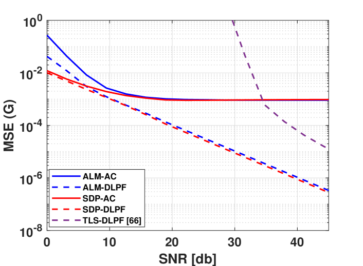
(a)

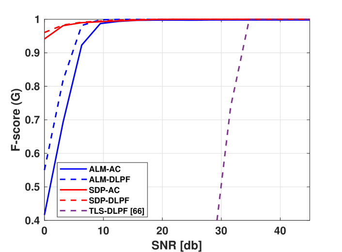
(b)

Figure 2: The MSE (a) and F-score (b) of the different estimators of ${\bf{G}}$ for IEEE 33-bus system, based on the DLPF measurement model.

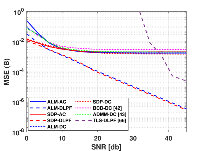
(a)

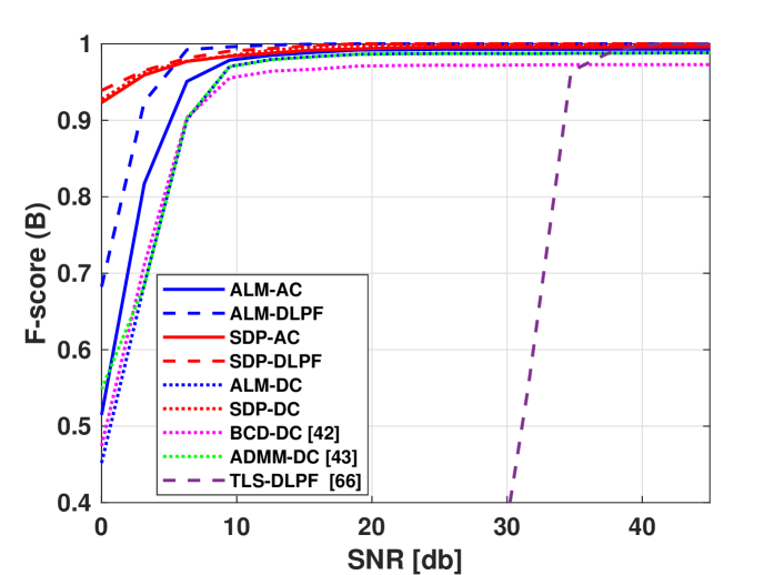
(b)

Figure 3: The MSE (a) and F-score (b) of the different estimators of ${\bf{B}}$ for IEEE 33-bus system, based on the DLPF measurement model.

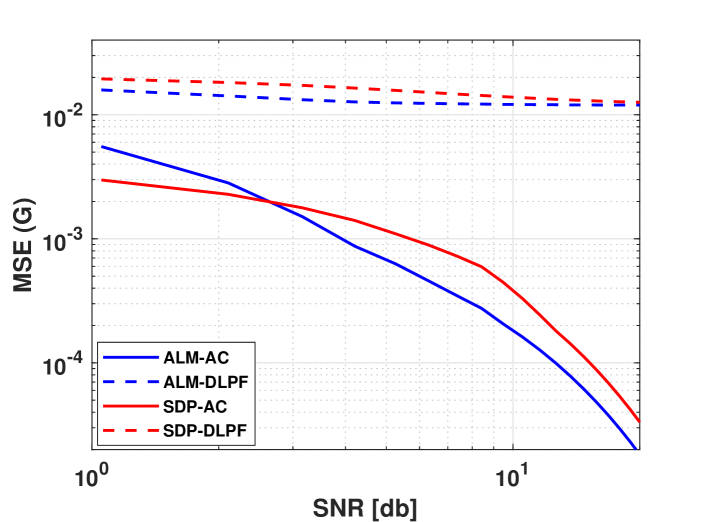
(a)

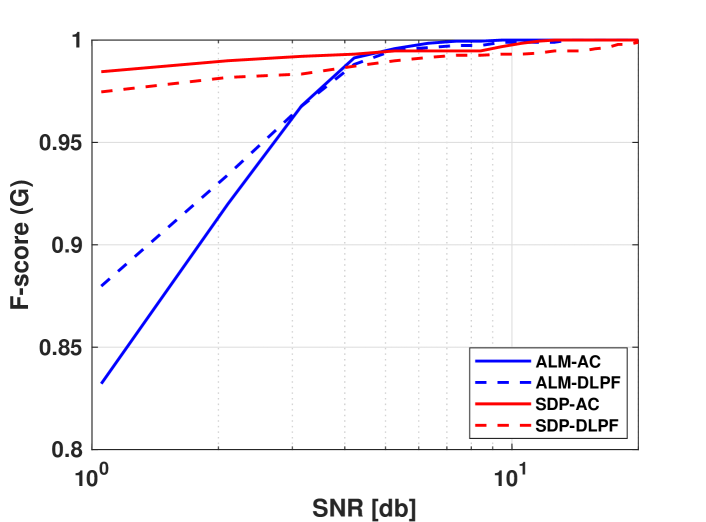
(b)

Figure 4: The MSE (a) and F-score (b) of the different estimators of ${\bf{G}}$ for IEEE 33-bus system, based on the AC measurement model.

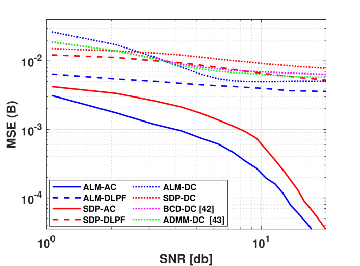
(a)

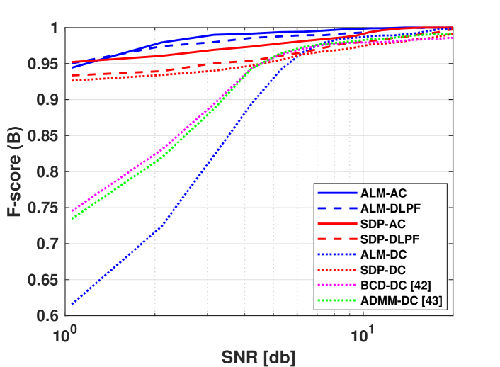
(b)

Figure 5: The MSE (a) and F-score (b) of the different estimators of ${\bf{B}}$ for IEEE 33-bus system, based on the AC measurement model.

VI Conclusions

In this paper, we propose novel methods for the estimation of sparse, complex-valued Laplacian matrices with a joint sparsity pattern. To effectively handle this joint sparsity, we formulate the CMLE for this estimation as the solution of a convex regularized and constrained optimization problem, and develop two associated algorithmic solutions: the SDP and ALM techniques. We analyze the computational complexity of the algorithms and their properties. In addition, we introduce a sample-covariance-based initialization approach for the ALM algorithm. We apply the proposed estimation methods to the problem of estimating the admittance matrix in a power system. In particular, we employ the proposed SDP and ALM algorithms for the three commonly-used linear and nonlinear observation models of the power flow equations. Numerical simulations, using the IEEE 33-bus model test case, show that the proposed SDP and ALM techniques successfully reconstruct the topology (i.e. the admittance matrix) and outperform existing approaches in terms of MSE and F-score. In general, the SDP is better in terms of F-score, while the ALM has a lower MSE and better run-time. The proposed initialization method also improves the performance of existing methods developed for the DC model, BCD [43] and ADMM algorithm [44]. Future work will involve extending the proposed methods to handle blind scenarios, where some voltage and/or power measurements are missing and need to be estimated as well. Additionally, it is important to develop performance bounds for the estimation approach. Furthermore, more GSP tools should be developed for handling the complex-valued Laplacian matrix, as they have extensive applications in signal processing.

References

- [1] M. Halihal and T. Routtenberg, “Estimation of the admittance matrix in power systems under Laplacian and physical constraints,” in Proc. of IEEE International Conference on Acoustics, Speech and Signal Processing (ICASSP), 2022, pp. 5972–5976.
- [2] L. Dabush and T. Routtenberg, “Verifying the smoothness of graph signals: A graph signal processing approach,” arXiv preprint arXiv: 2305.19618, 2023.
- [3] A. Sandryhaila and J. M. F. Moura, “Discrete signal processing on graphs: Frequency analysis,” IEEE Trans. Signal Process., vol. 62, no. 12, pp. 3042–3054, June 2014.
- [4] D. Shuman, Sunil K. Narang, P. Frossard, A. Ortega, and P. Vandergheynst, “The emerging field of signal processing on graphs: Extending high-dimensional data analysis to networks and other irregular domains,” IEEE Signal Process. Mag., vol. 30, no. 3, pp. 83–98, May 2013.
- [5] A. Amar and T. Routtenberg, “Widely-linear MMSE estimation of complex-valued graph signals,” IEEE Trans. Signal Process., vol. 71, pp. 1770–1785, 2023.
- [6] Z. Han, L. Wang, Z. Lin, and R. Zheng, “Formation control with size scaling via a complex Laplacian-based approach,” IEEE Trans. cybernetics, vol. 46, no. 10, pp. 2348–2359, 2015.
- [7] K. Tscherkaschin, B. Knoop, J. Rust, and S. Paul, “Design of a multi-core hardware architecture for consensus-based MIMO detection algorithms,” in Proc. of Asilomar, 2016, pp. 877–881.
- [8] T. Wu, A. Scaglione, and D. Arnold, “Complex-value spatio-temporal graph convolutional neural networks and its applications to electric power systems ai,” 2022.
- [9] E. Drayer and T. Routtenberg, “Detection of false data injection attacks in smart grids based on graph signal processing,” IEEE Systems Journal, vol. 14, no. 2, pp. 1886–1896, June 2020.
- [10] L. Dabush, A. Kroizer, and T. Routtenberg, “State estimation in partially observable power systems via graph signal processing tools,” Sensors, vol. 23, no. 3, pp. 1387, 2023.
- [11] J. K. Tugnait, “Graphical Lasso for high-dimensional complex Gaussian Graphical model selection,” in Proc. of IEEE International Conference on Acoustics, Speech and Signal Processing (ICASSP), 2019, pp. 2952–2956.
- [12] J. Friedman, T. Hastie, and R. Tibshirani, “Sparse inverse covariance estimation with the graphical Lasso,” Biostatistics, vol. 9, no. 3, pp. 432–441, 12 2007.
- [13] O. Banerjee, L. El Ghaoui, and A. d’Aspremont, “Model selection through sparse maximum likelihood estimation for multivariate Gaussian or binary data,” J. Mach. Learn. Res., vol. 9, pp. 485–516, jun 2008.
- [14] M. Rahul and H. Trevor, “The graphical Lasso: New insights and alternatives,” Journal of statistics, vol. 6, pp. 2125–2149, 2011.
- [15] H. E. Egilmez, E. Pavez, and A. Ortega, “Graph learning from data under structural and Laplacian constraints,” IEEE J. Sel. Top. Signal Process., vol. 11, no. 6, pp. 825–841, Sept. 2017.
- [16] J. Ying, J. M. Cardoso, and D. Palomar, “Minimax estimation of Laplacian constrained precision matrices,” in Proc. of the International Conference on Artificial Intelligence and Statistics, 2021, vol. 130 of PMLR, pp. 3736–3744.
- [17] Y. Medvedovsky, E. Treister, and T. Routtenberg, “Efficient graph laplacian estimation by a proximal newton approach,” arXiv preprint arXiv:2302.06434, 2023.
- [18] X. Dong, D. Thanou, P. Frossard, and P. Vandergheynst, “Learning Laplacian matrix in smooth graph signal representations,” IEEE Trans. Signal Process., vol. 64, no. 23, pp. 6160–6173, 2016.
- [19] V. Kalofolias, “How to learn a graph from smooth signals,” in Proc. of Artificial intelligence and statistics. PMLR, 2016, pp. 920–929.
- [20] P. C. Chepuri, S. Liu, G. Leus, and A. O. Hero, “Learning sparse graphs under smoothness prior,” in Proc. of IEEE International Conference on Acoustics, Speech and Signal Processing (ICASSP), 2017, pp. 6508–6512.
- [21] M. Golbabaee and P. Vandergheynst, “Hyperspectral image compressed sensing via low-rank and joint-sparse matrix recovery,” in Proc. of IEEE International Conference on Acoustics, Speech and Signal Processing (ICASSP), 2012, pp. 2741–2744.
- [22] L. Sun, J. Liu, J. Chen, and J. Ye, “Efficient recovery of jointly sparse vectors,” in Proc. of Advances in Neural Information Processing Systems. 2009, vol. 22, Curran Associates, Inc.
- [23] A. Hjørungnes, Complex-Valued Matrix Derivatives: With Applications in Signal Processing and Communications, Cambridge University Press, 2011.
- [24] A. Abur and A. Gomez-Exposito, Power System State Estimation: Theory and Implementation, Marcel Dekker, 2004.
- [25] G. B. Giannakis, V. Kekatos, N. Gatsis, S. J. Kim, H. Zhu, and B. F. Wollenberg, “Monitoring and optimization for power grids: A signal processing perspective,” IEEE Signal Process. Magazine, vol. 30, no. 5, pp. 107–128, Sept. 2013.
- [26] A. Primadianto and C.N. Lu, “A review on distribution system state estimation,” IEEE Trans. Power Systems, vol. 32, no. 5, pp. 3875–3883, 2017.
- [27] A. Tajer, S. Sihag, and K. Alnajjar, “Non-linear state recovery in power system under bad data and cyber attacks,” Journal of Modern Power Systems and Clean Energy, vol. 7, no. 5, pp. 1071–1080, 2019.
- [28] S. Cui, Z. Han, S. Kar, T. T. Kim, H. V. Poor, and A. Tajer, “Coordinated data-injection attack and detection in the smart grid: A detailed look at enriching detection solutions,” IEEE Signal Process. Magazine, vol. 29, no. 5, pp. 106–115, Sept. 2012.
- [29] G. Morgenstern, J. Kim, J. Anderson, G. Zussman, and T. Routtenberg, “Protection against graph-based false data injection attacks on power systems,” arXiv preprint arXiv:2304.10801, 2023.
- [30] M. Pourali and A. Mosleh, “A functional sensor placement optimization method for power systems health monitoring,” in Proc. of IEEE Industry Applications Society Annual Meeting, 2012, pp. 1–10.
- [31] E. Dall’Anese, H. Zhu, and G. B. Giannakis, “Distributed optimal power flow for smart microgrids,” IEEE Trans. Smart Grid, vol. 4, no. 3, pp. 1464–1475, 2013.
- [32] A. Zamzam, X. Fu, and N.D. Sidiropoulos, “Data-driven learning-based optimization for distribution system state estimation,” IEEE Trans. Power Systems, vol. PP, pp. 1–1, 04 2019.
- [33] S. Soltan, D. Mazauric, and G. Zussman, “Analysis of failures in power grids,” IEEE Trans. Control of Network Systems, vol. 4, no. 2, pp. 288–300, 2017.
- [34] D. Deka, S. Backhaus, and M. Chertkov, “Estimating distribution grid topologies: A graphical learning based approach,” in Proc. of Power Systems Computation Conference (PSCC), 2016, pp. 1–7.
- [35] S. Grotas, Y. Yakoby, I. Gera, and T. Routtenberg, “Power systems topology and state estimation by graph blind source separation,” IEEE Trans. Signal Process., vol. 67, no. 8, pp. 2036–2051, Apr. 2019.
- [36] I. Gera, Y. Yakoby, and T. Routtenberg, “Blind estimation of states and topology (BEST) in power systems,” in Proc. of IEEE Global Conference on Signal and Information Processing (GlobalSIP), Nov. 2017, pp. 1080–1084.
- [37] D. Deka, S. Backhaus, and M. Chertkov, “Structure learning in power distribution networks,” IEEE Trans. Control of Network Systems, vol. 5, no. 3, pp. 1061–1074, Sept. 2018.
- [38] S. Park, D. Deka, and M. Chertkov, “Exact topology and parameter estimation in distribution grids with minimal observability,” in Proc. of Power Systems Computation Conference (PSCC), 2018.
- [39] R. Emami and A. Abur, “Tracking changes in the external network model,” in Proc. of North American Power Symposium 2010, Sep. 2010, pp. 1–6.
- [40] Y. Sharon, A. M. Annaswamy, A. L. Motto, and A. Chakraborty, “Topology identification in distribution network with limited measurements,” in Proc. of PES Innovative Smart Grid Technologies (ISGT), Jan. 2012, pp. 1–6.
- [41] S. Shaked and T. Routtenberg, “Identification of edge disconnections in networks based on graph filter outputs,” IEEE Trans. Signal Inf. Process. Netw., vol. 7, pp. 578–594, 2021.
- [42] Y. Zhao, J. Chen, and H. V. Poor, “A learning-to-infer method for real-time power grid multi-line outage identification,” IEEE Trans. Smart Grid, vol. 11, no. 1, pp. 555–564, 2020.
- [43] X. Li, H. V. Poor, and A. Scaglione, “Blind topology identification for power systems,” in Proc. of IEEE International Conference on Smart Grid Communications (SmartGridComm), Oct. 2013, pp. 91–96.
- [44] A. Anwar, A. Mahmood, and M. Pickering, “Estimation of smart grid topology using SCADA measurements,” in Proc. of SmartGridComm, Nov. 2016, pp. 539–544.
- [45] V. Kekatos, G. B. Giannakis, and R. Baldick, “Online energy price matrix factorization for power grid topology tracking,” IEEE Trans. Smart Grid, vol. 7, no. 3, pp. 1239–1248, May 2016.
- [46] S. Xie, J. Yang, K. Xie, Y. Liu, and Z. He, “Low-sparsity unobservable attacks against smart grid: Attack exposure analysis and a data-driven attack scheme,” IEEE Access, vol. 5, pp. 8183–8193, 2017.
- [47] M. J. Choi, V. Y. Tan, A. Anandkumar, and A. S. Willsky, “Learning latent tree graphical models,” J. Mach. Learn. Res., vol. 12, no. null, pp. 1771–1812, jul 2011.
- [48] S. Mousavi, S. Seyed, F. Aminifar, and S. Afsharnia, “Parameter estimation of multiterminal transmission lines using joint PMU and SCADA data,” IEEE Trans. Power Delivery, vol. 30, no. 3, pp. 1077–1085, 2015.
- [49] K. Dasgupta and S. A. Soman, “Line parameter estimation using phasor measurements by the total least squares approach,” in Proc. of IEEE Power & Energy Society General Meeting, 2013, pp. 1–5.
- [50] N. Parikh S. Boyd and J. Eckstein E. Chu, B. Peleato, “Distributed optimization and statistical learning via the alternating direction method of multipliers,” IEEE Machine Learning, vol. 3, no. 1, pp. 1–122, 2011.
- [51] A. Monticelli, State Estimation in Electric Power Systems: A Generalized Approach, pp. 39–61,91–101,161–199, Springer US, Boston, MA, 1999.
- [52] R. A. Horn and C. R. Johnson, Matrix Analysis, Cambridge University Press, New York, NY, USA, 2nd edition, 2012.
- [53] Z. Wang, A. Scaglione, and R. J. Thomas, “Generating statistically correct random topologies for testing smart grid communication and control networks,” IEEE Trans. Smart Grid, vol. 1, no. 1, pp. 28–39, June 2010.
- [54] “Power systems test case archive,” .
- [55] M. Sokolova and G. Lapalme, “A systematic analysis of performance measures for classification tasks,” Information Processing and Management, vol. 45, pp. 427–437, 07 2009.
- [56] T. J. Moore, B. M. Sadler, and R. J. Kozick, “Maximum-likelihood estimation, the Cramr-Rao bound, and the method of scoring with parameter constraints,” IEEE Trans. Signal Process., vol. 56, no. 3, pp. 895–908, Mar. 2008.
- [57] E. Nitzan, T. Routtenberg, and J. Tabrikian, “Cramr-Rao bound for constrained parameter estimation using Lehmann-unbiasedness,,” IEEE Trans. Signal Process., vol. 67, no. 3, pp. 753–768, Feb. 2019.
- [58] R. Dai and J. Yang, “Seismic inversion with l2,0-norm joint-sparse constraint on multi-trace impedance model,” Scientific Reports, vol. 12, 12 2022.
- [59] R. Tibshirani, “Regression shrinkage and selection via the Lasso,” Journal of the Royal Statistical Society (Series B), vol. 58, pp. 267–288, 1996.
- [60] L. Zhao, Y. Wang, S. Kumar, and D. A. Palomar, “Optimization algorithms for graph Laplacian estimation via ADMM and MM,” IEEE Trans. Signal Process., vol. 67, no. 16, pp. 4231–4244, 2019.
- [61] S. Boyd and L. Vandenberghe, Convex Optimization, Cambridge University Press, New York, NY, USA, 2004.
- [62] M. Grant and S. Boyd, “CVX: Matlab software for disciplined convex programming, version 2.0,” Aug. 2012.
- [63] Y. Yuan, S. H. Low, O. Ardakanian, and C. J. Tomlin, “Inverse power flow problem,” IEEE Trans. Control of Network Systems, vol. 10, no. 1, pp. 261–273, 2023.
- [64] A. G. Phadke and J. S. Thorp, Synchronized Phasor Measurements and Their Applications, New York: Springer Science, 2008.
- [65] J. Yang, N. Zhang, C. Kang, and Q. Xia, “A state-independent linear power flow model with accurate estimation of voltage magnitude,” IEEE Trans. Power Systems, vol. 32, no. 5, pp. 3607–3617, 2017.
- [66] J. Zhang, P. Wang, and N. Zhang, “Distribution network admittance matrix estimation with linear regression,” IEEE Trans. Power Systems, vol. 36, no. 5, pp. 4896–4899, 2021.
- [67] B. Donmez and A. Abur, “Sparse estimation based external system line outage detection,” in Proc. of Power Systems Computation Conference (PSCC), 2016, pp. 1–6.
- [68] R. D. Zimmerman, C. E. Murillo-Sánchez, and R. J. Thomas, “MATPOWER: Steady-state operations, planning, and analysis tools for power systems research and education,” IEEE Trans. Power Systems, vol. 26, no. 1, pp. 12–19, 2011.