A Novel Joint Angle-Range-Velocity Estimation Method for MIMO-OFDM ISAC Systems

Abstract

Integrated sensing and communications (ISAC) is emerging as a key technique for next-generation wireless systems. In order to expedite the practical implementation of ISAC within pervasive mobile networks, it is essential to equip widely-deployed base stations with radar sensing capabilities. Thus, the utilization of standardized multiple-input multiple-output (MIMO) orthogonal frequency division multiplexing (OFDM) hardware architectures and waveforms becomes pivotal for realizing seamless integration of effective communication and sensing functionalities. In this paper, we introduce a novel joint angle-range-velocity estimation algorithm for the MIMO-OFDM ISAC system. This approach exclusively depends on conventional MIMO-OFDM communication waveforms, which are widely adopted in wireless communications. Specifically, the angle-range-velocity information of potential targets is jointly extracted by utilizing all the received echo signals within a coherent processing interval (CPI). Therefore, the proposed joint estimation algorithm can achieve larger processing gains and higher resolution by fully exploiting echo signals and jointly estimating the angle-range-velocity information. Theoretical analysis for maximum unambiguous range, resolution, and processing gains are provided to verify the advantages of the proposed joint estimation algorithm. Finally, extensive numerical experiments are presented to demonstrate that the proposed joint estimation approach can achieve significantly lower root-mean-square-error (RMSE) of angle/range/velocity estimation for both single-target and multi-target scenarios.

I Introduction

Next-generation wireless systems are expected to develop beyond traditional communication service providers and further facilitate a series of innovative applications, such as intelligent transportation, manufacturing, healthcare, etc. These emerging applications not only impose higher demands on communication performance but also require more robust sensing capabilities. In addition, with the exponential growth of wireless devices and communication demands, spectral resources are becoming increasingly scarce. The radar frequency bands, which have large portions of the available spectrum, are therefore regarded as one promising choice for communication usage. From a technical point of view, the technology trend of wireless communication and radar sensing also shows a high degree of consistency: The pursuit of higher frequencies, wider bandwidths, larger antenna arrays, more attention to line-of-sight channels, and distributed dense deployment. Therefore, wireless communication and radar sensing exhibit more and more commonality and similarity in system design, hardware platform, signal processing, etc., which lays a solid technical foundation for the integration of these two functionalities. Owing to these factors, the emerging integrated sensing and communications (ISAC), which focuses on the coexistence, cooperation, and co-design of communication and sensing systems, has recently been recognized as one of the key enabling technologies for the sixth generation (6G) wireless systems [1] and has aroused extensive research attentions from both academia and industry [2]-[4].

Many types of ISAC systems have been proposed and they can be generally divided into traditional radar system based, communication system based, or dual-functional systems that require special customization. In specific, radar-based ISAC systems focus on embedding communication symbols into existing radar sensing signals, e.g., linear frequency modulated continuous wave (LFMCW) [5] and frequency-hopping (FH) radar [6]. Communication-based ISAC systems rely on existing hardware architectures and signal structures for communications to perform dual-functional tasks, e.g., the investigations based on 802.11ad standard waveforms [7] and the studies for perceptive mobile networks (PMNs) [8], [9]. In addition, the dual-functional systems not restricted to existing radar/communication infrastructures have also been investigated [10], [11]. Considering that the ubiquitous wireless communication networks, communication-based designs will greatly facilitate the practical development of ISAC. Therefore, the investigation of utilizing communication transceiver architectures and waveforms to empower wireless networks with sensing capabilities is pivotal.

In existing commercial wireless communication networks, orthogonal frequency division multiplexing (OFDM) has been widely adopted as the dominant waveform. Benefiting from its capabilities to overcome frequency selective fading and support high spectral efficiency, OFDM waveforms provide a much higher information transmission rate for wireless communications. On the other hand, OFDM waveforms provide satisfactory radar sensing performance, e.g., by harnessing frequency diversity, OFDM waveforms can enhance target detection [12], [13] or parameter estimation [14]; by utilizing the cyclic prefixed (CP) structure, OFDM waveforms can entirely eliminate the inter-range-cell interference for range reconstruction [15], [16]. Therefore, the OFDM waveform has been recognized as an attractive candidate for realizing ISAC in practice. Considering that OFDM waveform is communication-oriented, how to realize high-performance radar sensing functionality based on existing OFDM communication systems is a key task to facilitate practical ISAC applications.

Many researchers have explored OFDM waveform design and echo signal processing algorithms for ISAC systems, in which the dual-functional OFDM waveform is optimized to simultaneously perform single/multiple-user communications and target detection/estimation/tracking. In specific, to realize target parameter estimation using OFDM communication signals, the seminal work [17] presented a novel echo signal processing algorithm for estimating the range and velocity of potential targets. Then, super-resolution methods were presented in [18]-[20], and a deep-learning based method for terahertz systems was developed in [21]. In addition, the power allocation problem was investigated [22]-[24] in order to achieve a better performance trade-off for OFDM ISAC systems. While the aforementioned studies [17]-[24] have verified the potential viability of employing OFDM waveform for the implementation of ISAC, their scope was limited to exploring a scenario involving a single-antenna transmitter.

Multi-input multi-output (MIMO) architecture has been widely employed in both communication and radar sensing systems, and is therefore regarded as one key feature of future ISAC systems. The MIMO architecture provides additional spatial degrees-of-freedom (DoFs), which can be exploited to achieve spatial multiplexing, spatial diversity, and beamforming gain for both communication and radar sensing [25], [26]. However, when equipped with multiple transmit antennas in OFDM ISAC, the emitted dual-functional transmit waveforms which carry communication symbols of randomness will be mixed together in the spatial domain coupling with target parameters. In the sequel, different from the single transmit antenna scenario, the direct separation of random communication symbols and radar parameters is not feasible, thereby leading to substantial challenges in the estimation of target parameters. Therefore, the estimation of potential target parameters in MIMO-OFDM ISAC systems necessitates the implementation of advanced echo signal processing algorithms.

In order to avoid the mixture of signals emitted from different antennas, the authors in [27] proposed to allocate different subcarriers to each antenna, i.e., the subcarriers are non-overlapping among the antennas, which makes the subsequent parameter estimation much easier. However, since frequency resources are not fully exploited, it is obvious that the communication capacity will be significantly reduced. Later, the work [8] proposed a compressed sensing (CS) based method for tackling the estimation of utilizing typical MIMO-OFDM communication signals. This approach is usually computationally prohibitive. More recently, works [28] and [29] introduced a novel estimation strategy, in which the angle information is first estimated and then the range and velocity are estimated. Particularly, the authors in paper [28] employed a maximum likelihood (ML) approach for extracting the range and velocity parameters, which is done by searching over the entire target range-velocity parameter space. Such an approach would involve high complexity. In paper [29], a suboptimal but more computationally efficient approach based on discrete Fourier transform (DFT) spectrum analysis is proposed. Although this approach fully utilizes spatial and frequency resources in MIMO-OFDM waveforms and is computationally friendly, the estimation of angle and range only exploits the received echo signals during one OFDM symbol. Compared with traditional radar sensing algorithms that are usually performed during one coherent processing interval (CPI) with multiple OFDM symbols, this approach [29] will suffer from lower signal processing gains. Moreover, the angle-range-velocity of potential targets is successively estimated in [28], [29], which will inevitably lead to error propagation on parameter estimation. Therefore, it is important to conduct further investigations into echo signal processing and parameter estimation algorithms in MIMO-OFDM ISAC systems.

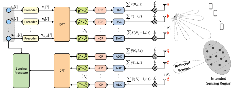
Figure 1: The considered MIMO-OFDM ISAC system.

Motivated by the above findings, in this paper we focus on echo signal processing for better parameter estimation performance in MIMO-OFDM ISAC systems. In particular, we consider a typical MIMO-OFDM ISAC system, in which a multi-antenna base station (BS) transmits conventional OFDM communication waveforms to simultaneously serve multiple communication users and estimate the parameters of multiple point-like targets via processing received echo signals. Our goal is to propose a joint angle-range-velocity estimation approach to fully exploit available information in spatial, frequency, and temporal domains of the MIMO-OFDM echo signals. The main contributions of this paper are presented as follows.

• First, we propose a novel estimation method for processing the echoes of widely adopted MIMO-OFDM communication waveforms, in which target angle-range-velocity are jointly estimated by fully utilizing all the echo signals of one CPI. In specific, toward the 3-dimensional echo data cube of spatial-delay-Doppler domains, DFT-based spectrum analysis is first conducted along the spatial dimension to reallocate the signal power according to the percentage of angular components. Then, a novel division approach is proposed to remove the random communication symbols contained in the cube. Afterward, spectrum analysis along the delay and Doppler dimensions is performed. Finally, the angle-range-velocity parameters are jointly estimated with peak finding. This joint estimation strategy can bring substantial processing gains compared with the existing approach that relies solely on the part of the echo cube. Moreover, through joint estimation from three dimensions instead of successively determining its parameters, the sensing resolution can be significantly improved.

• Next, we provide theoretical analysis for the maximum unambiguous range, resolution, and signal-to-noise ratio (SNR) processing gain achieved by the proposed joint estimation approach, from which we gain valuable insights about the achievable sensing performance improvements.

• Finally, simulation results are presented to validate the feasibility and advantages of the proposed joint estimation method. Compared to existing work, the proposed method provides superior performance for angle-range-velocity estimation in terms of root-mean-squared-error (RMSE) and SNR gains. Moreover, we show that, without sacrificing any communication performance, there is subtle sensing loss in utilizing conventional MIMO-OFDM communication waveform with the proposed estimation method compared to pure radar system using typical LFMCW waveform.

Notation: Lower-case, boldface lower-case, and upper-case letters indicate scalars, column vectors, and matrices, respectively. $(\cdot)^{T}$ and $(\cdot)^{H}$ denote the transpose and transpose-conjugate operations, respectively. $\mathbb{E}\{\cdot\}$ represents statistical expectation. $|a|$ is the magnitude of a scalar $a$. $\mathbb{Z}$ and $\mathbb{C}$ denote the set of integers and complex numbers, respectively. $\sqrt{a}$ returns the square root of scalar $a$. $\lfloor\cdot\rfloor$ rounds a real number to the nearest integer less than or equal to it.

II System Model

We consider a mono-static MIMO-OFDM ISAC system as illustrated in Fig. 1, in which a dual-functional BS equipped with two separate uniform linear arrays (ULAs) of $N_{\mathrm{t}}$ transmit antennas and $N_{\mathrm{r}}$ receive antennas simultaneously performs downlink multi-user communications and target parameter estimation. We assume that the BS operates in a full-duplex mode with perfect self-interference (SI) cancellation with the aid of advanced full-duplex techniques [30]-[32]. Specifically, the BS transmits OFDM waveforms to communicate with $K$ single-antenna users and sense multiple point-like targets, and meanwhile processes the received echo signals for estimating the angle-range-velocity information of potential targets.

II-A Transmitted Signal Model

In the considered OFDM system, the central carrier frequency is $f_{\mathrm{c}}$ and the wavelength is $\lambda_{\mathrm{c}}=c/f_{\mathrm{c}}$, where $c$ denotes the speed of light. There are $N_{\mathrm{s}}$-subcarriers with frequency spacing $\Delta f=1/T_{\mathrm{d}}$, where $T_{\mathrm{d}}$ is the OFDM symbol duration. We denote the communication symbol vector of the $i$-th subcarrier at the $l$-th symbol-slot as $\mathbf{s}_{i}[l]\in\mathbb{C}^{K}$, $i=0,\ldots,N_{\mathrm{s}}-1$, $l=0,\ldots,L-1$, where $L$ is the frame length of one CPI. Each element of $\mathbf{s}_{i}[l]$ is independently selected from quadrature amplitude modulation (QAM) constellation, $\mathbb{E}\{\mathbf{s}_{i}[l]\}=\mathbf{0}$ and $\mathbb{E}\{\mathbf{s}_{i}[l]\mathbf{s}^{H}_{i}[l]\}=\mathbf{I}_{K}$. The transmitted symbols are firstly precoded through precoders $\mathbf{W}_{i}\triangleq[\mathbf{w}_{i,1},\ldots,\mathbf{w}_{i,K}]\in\mathbb{C}^{N_{\mathrm{t}}\times K}$, $\forall i$, in order to focus the beams towards the communication users and potential targets. Thus, the transmitted signal on the $i$-th subcarrier during the $l$-th OFDM symbol can be expressed as

$$\mathbf{x}_{i}[l]\triangleq\left[\begin{array}[]{lccc}&x(0,i,l)\\ &x(1,i,l)\\ &\ldots\\ &x(N_{\mathrm{t}}-1,i,l)\end{array}\right]=\mathbf{W}_{i}\mathbf{s}_{i}[l],$$ (1)

where $x(n,i,l)$ denotes the signal transmitted by the $n$-th antenna, $n=0,\ldots,N_{\mathrm{t}}-1$.

As described in Fig. 1, the baseband signals (1) in the frequency domain are transformed into the temporal domain by $N_{\mathrm{s}}$-point inverse discrete Fourier transform (IDFT). Then, a CP of $N_{\mathrm{cp}}$ points and $T_{\mathrm{cp}}$ duration is inserted in order to avoid inter-symbol interference (ISI) for both communication and sensing. We know that the CP length should be greater than the channel impulse response length to avoid ISI for downlink communications. Meanwhile, in order to eliminate ISI at the sensing receiver, the CP duration should also be larger than the roundtrip delay between the BS and the furthest target. Then, after being processed by digital-to-analog converters (DACs), the baseband analog signal transmitted by the $n$-th antenna on the $i$-th subcarrier is expressed as

$$\widetilde{x}(n,i,t)\triangleq\sum_{l=0}^{L-1}x(n,i,l)e^{\jmath 2\pi i\Delta ft}\mathrm{rect}\left(\frac{t-lT}{T}\right),$$ (2)

where $T\triangleq T_{\mathrm{d}}+T_{\mathrm{cp}}$ is the total symbol duration and $\mathrm{rect}({t}/{T})$ denotes a rectangular pulse of duration $T$. Finally, the baseband analog signal is up-converted to the radio frequency (RF) domain via $N_{\mathrm{t}}$ RF chains with carrier frequency $f_{\mathrm{c}}$ and then emitted through the antennas.

II-B Communication Signal Model

After propagating through downlink communication channels, the OFDM signals are received by the single-antenna users and then demodulated into communication symbols. In particular, the communication receiver employs a series of operations including down-converting, analog-to-digital converting (ADC), removing the CP, and $N_{\mathrm{s}}$-point DFT to process the received communication signals. For the $k$-th user, the frequency-domain signal on the $i$-th subcarrier during the $l$-th OFDM symbol can be written as

$$y_{i,k}[l]\triangleq\mathbf{h}_{i,k}^{H}\mathbf{W}_{i}\mathbf{s}_{i}[l]+z_{i,k}[l],$$ (3)

where the vector $\mathbf{h}_{i,k}\in\mathbb{C}^{N_{\mathrm{t}}}$ denotes the frequency domain channel between the BS and the $k$-th user, and the scalar $z_{i,k}\in\mathcal{CN}(0,\sigma_{\mathrm{c}}^{2})$ denotes the additive white Gaussian noise (AWGN). In order to achieve satisfactory communication and sensing performance, the precoders $\mathbf{W}_{i}$ should be properly designed to direct the beampattern toward users and interested targets, as well as suppressing multi-user interference (MUI). While the precoder/beamforming design for ISAC systems has been extensively investigated [2]-[4], in this paper we focus on the radar echo signal processing method to provide satisfactory parameter estimation performance based on MIMO-OFDM communication waveforms.

II-C Sensing Signal Model

From the radar sensing perspective, the dual-functional BS attempts to estimate the angle-range-velocity information of multiple point-like targets by processing the received echo signals. We assume that there are $Q$ targets within the areas of interest, in which the angle-range-velocity information of the $q$-th target is denoted as $\theta_{q}$, $d_{q}$, and $v_{q}$, respectively, $q\in\mathcal{Q}\triangleq\{1,\ldots,Q\}$. It is noted that the direction of arrival (DoA) and the direction of departure (DoD) are the same as $\theta_{q}$ in the considered mono-static ISAC system.

The transmitted OFDM signals will reach the $Q$ targets and be reflected back to the receive antennas of the BS. In specific, the transmitted OFDM signals will experience round-trip path-loss and propagation delay, and the Doppler frequency shift before arriving at the receive antenna array. Thus, the baseband echo signal received by the $m$-th antenna can be expressed as

$$\widetilde{y}(m,t)\triangleq \sum_{q=1}^{Q}\sum_{i=0}^{N_{\mathrm{s}}-1}\beta_{q}\sqrt{\mathrm{PL}(2d_{q})}\sum_{n=0}^{N_{\mathrm{t}}-1}\big{[}\widetilde{x}(n,i,t-2d_{q}/c)$$

$$e^{{-\jmath 2\pi nd_{\mathrm{t}}\sin\theta_{q}}/{\lambda_{\mathrm{c}}}}e^{{-\jmath 2\pi md_{\mathrm{r}}\sin\theta_{q}}/{\lambda_{\mathrm{c}}}}e^{\jmath 2\pi f_{\mathrm{D},q}t}\big{]}$$

$$+\widetilde{z}(m,t),$$ (4)

where $m=0,\ldots,N_{\mathrm{r}}-1$ is the index of receive antennas, the scalar $\beta_{q}$ denotes the reflection coefficient of the $q$-th target with power $\mathbb{E}\{|\beta_{q}|^{2}\}=\sigma_{\beta}^{2}$, the scalar $\mathrm{PL}(d)\triangleq c_{0}({d}/{d_{0}})^{-\alpha}$ represents the distance-dependent path-loss with $c_{0}$ being the loss at the reference distance $d_{0}$, $d$ the link distance and $\alpha$ the path-loss exponent, the scalar $d_{\mathrm{t}}$ is the transmit antenna spacing, the scalar $d_{\mathrm{r}}$ is the receive antenna spacing, $f_{\mathrm{D},q}\triangleq{2v_{q}f_{\mathrm{c}}}/{c}$ is the Doppler frequency of the $q$-th target, and the scalar $\widetilde{z}(m,t)$ is the independently and identically distributed (i.i.d.) AWGN at the receive antennas. It is generally assumed that the channel scattering coefficients, the reflection coefficients and the angle-range-velocity of targets are constant during one CPI. Considering that the signal bandwidth is usually much smaller than the central carrier frequency, the phase shifts along the spatial axis are assumed to be identical on all subcarriers and the Doppler frequency shift within one OFDM symbol is also assumed to be identical on all subcarriers. In addition, only the first-order reflection from the target is considered due to high attenuation.

As presented in Fig. 1, the received echo signals (4) are processed by ADCs with the sampling frequency $F_{\mathrm{s}}\triangleq N_{\mathrm{s}}\Delta f$ and removing CP. Then, the digital sampled echo signals without CP of the $l$-th symbol-slot can be written as

$$\widehat{y}(m,j,l)\triangleq \widetilde{y}(m,lT+j\frac{1}{F_{\mathrm{s}}}+T_{\mathrm{cp}})$$ (5)

$$= \sum_{q=1}^{Q}\sum_{i=0}^{N_{\mathrm{s}}-1}\beta_{q}\sqrt{\mathrm{PL}(2d_{q})}\sum_{n=0}^{N_{\mathrm{t}}-1}\big{[}x(n,i,l)$$

$$e^{\jmath 2\pi i\Delta f(lT+j\frac{1}{F_{\mathrm{s}}}+T_{\mathrm{cp}}-2d_{q}/c)}e^{{-\jmath 2\pi nd_{\mathrm{t}}\sin\theta_{q}}/{\lambda_{\mathrm{c}}}}$$

$$e^{{-\jmath 2\pi md_{\mathrm{r}}\sin\theta_{q}}/{\lambda_{\mathrm{c}}}}e^{\jmath 2\pi f_{\mathrm{D},q}(lT+j\frac{1}{F_{\mathrm{s}}}+T_{\mathrm{cp}})}\big{]}$$

$$+\widetilde{z}(m,lT+j\frac{1}{F_{\mathrm{s}}}+T_{\mathrm{cp}}),$$

where $j$ is the sample index, $j=0,\ldots,N_{\mathrm{s}}-1$. Finally, by applying an $N_{\mathrm{s}}$-point DFT along the sample index dimension, the echo signal received by the $m$-th receive antenna on the $i$-th subcarrier can be formulated as

$$y(m,i,l)\triangleq \sum_{q=1}^{Q}\beta_{q}\sqrt{\mathrm{PL}(2d_{q})}\mathbf{a}^{H}\left(\omega_{\mathrm{t}}(\theta_{q})\right)\mathbf{x}_{i}[l]$$ (6)

$$e^{\jmath m\omega_{\mathrm{r}}(\theta_{q})}e^{\jmath i\omega_{\mathrm{d}}(d_{q})}e^{\jmath l\omega_{\mathrm{v}}(v_{q})}+z(m,i,l),$$

where $z(m,i,l)\sim\mathcal{CN}(0,\sigma_{\mathrm{s}}^{2})$ denotes the DFT of the AWGN $\widetilde{z}(m,lT+j\frac{1}{F_{\mathrm{s}}}+T_{\mathrm{cp}})$ during the $l$-th OFDM symbol. For conciseness, in (6) we respectively define the transmit steering vector $\mathbf{a}(\omega)$, and the digital frequencies related to the DoD with respect to transmit antennas, the DoA with respect to receive antennas, the range and the velocity of the $q$-th target as

$$\mathbf{a}(\omega) \triangleq[e^{\jmath 0},e^{\jmath 1\omega},\ldots,e^{\jmath(N_{\mathrm{t}}-1)\omega}]^{T},$$ (7a)

$$\omega_{\mathrm{t}}(\theta_{q}) \triangleq 2\pi d_{\mathrm{t}}\sin\theta_{q}/\lambda_{\mathrm{c}},$$ (7b)

$$\omega_{\mathrm{r}}(\theta_{q}) \triangleq-2\pi d_{\mathrm{r}}\sin\theta_{q}/\lambda_{\mathrm{c}},$$ (7c)

$$\omega_{\mathrm{d}}(d_{q}) \triangleq-4\pi\Delta f{d_{q}}/{c},$$ (7d)

$$\omega_{\mathrm{v}}(v_{q}) \triangleq 4\pi Tv_{q}f_{\mathrm{c}}/c.$$ (7e)

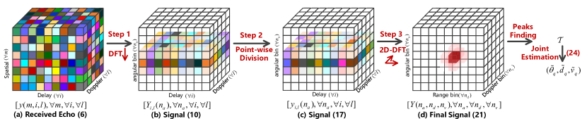
Figure 2: The processing flowchart of the proposed joint estimation method.

For radar sensing functionality, in this paper we focus on estimating the angle-range-velocity information of the targets based on the received echo signal $y(m,i,l)$ in (6). The angle $\theta_{q}$, the range $d_{q}$, and the velocity $v_{q}$ of the targets are determined by the digital frequencies $\omega_{\text{r}}(\theta_{q})$, $\omega_{\mathrm{d}}(d_{q})$, and $\omega_{\mathrm{v}}(v_{q})$, respectively. We note that radar target parameter estimation is performed during one CPI using the data cube of received echo signals as modeled in (6), which can be visually illustrated in Fig. 2. It is clear that the data cube consists of three dimensions, i.e., the spatial-delay-Doppler dimensions that are related to the receive antennas, the carriers, and the OFDM symbols, respectively, from which we attempt to extract the angle-range-velocity information of potential targets. However, we observe that the sinusoidal functions with angle/range/velocity-dependent digital frequencies are multiplied by the signal-dependent coefficients $\mathbf{a}^{H}(\omega_{\text{t}}(\theta_{q}))\mathbf{x}_{i}[l]$, which are determined by the transmitted dual-functional signals and the DoDs of potential targets. Therefore, the angle-range-velocity information cannot be directly extracted from the data cube via typical spectrum analysis. In order to tackle this difficulty, we propose a novel joint angle-range-velocity estimation method to remove the influence of the signal-dependent coefficients and fully exploit the three-dimensional information of the data cube to improve the parameter estimation performance.

III Joint Angle-Range-Velocity Estimation

In this section, we focus on extracting the angle-range-velocity information of potential targets from the received echo signals $y(m,i,l),~{}\forall m,~{}\forall i,~{}\forall l$. A novel joint estimation method is proposed to fully exploit the data cube during one CPI and jointly estimate the angle-range-velocity information.

III-A Observations from the Echo Signals

To achieve better parameter estimation performance, we specifically examine the received echo signals $y(m,i,l)$ and its representation in Fig. 2. According to the signal model in (6), we have the following observations.

• Along the spatial dimension (i.e., along the axis of receive antennas $\{m=0,1,\ldots,N_{\text{r}}-1\}$), the echo signals can be regarded as the summation of $Q$ sinusoidal functions with the digital frequency being determined by the DoA $\theta_{q}$ and the constant amplitude.

• Along the delay dimension (i.e., along the axis of carriers $\{i=0,1,\ldots,N_{\text{s}}-1\}$), the echo signals are composed of $Q$ sinusoidal functions multiplied by different coefficients. Particularly, the digital frequencies along the delay dimension are determined by the range of potential target $d_{q}$ and the signal-dependent coefficient $\mathbf{a}^{H}\left(\omega_{\mathrm{t}}(\theta_{q})\right)\mathbf{x}_{i}[l]$.

• Along the Doppler dimension (i.e., along the axis of symbols $\{l=0,1,\ldots,L-1\}$), the echo signals also consist of $Q$ sinusoidal functions multiplied by different signal-dependent coefficients. In other words, the digital frequencies along the Doppler dimension are determined by the velocity of potential target $v_{q}$ and the signal-dependent coefficient $\mathbf{a}^{H}\left(\omega_{\mathrm{t}}(\theta_{q})\right)\mathbf{x}_{i}[l]$.

• As for the signal-dependent coefficient $\mathbf{a}^{H}(\omega_{\text{t}}(\theta_{q}))\mathbf{x}_{i}[l]$, it is related to the DoD of potential target $\theta_{q}$ to be estimated and the transmitted signal $\mathbf{x}_{i}[l]$. As presented in (1), the dual-functional transmitted signal $\mathbf{x}_{i}[l]$ is a function of transmitted communication symbols, which are randomly generated. Therefore, the signal-dependent coefficient $\mathbf{a}^{H}(\omega_{\text{t}}(\theta_{q}))\mathbf{x}_{i}[l]$ will significantly influence the spectrum analysis for estimating the angle-range-velocity information of potential targets.

Based on the above observations, it is clear that the angle-range-velocity information is fused in different dimensions of the data cube. Moreover, the signal-dependent coefficient $\mathbf{a}^{H}(\omega_{\text{t}}(\theta_{q}))\mathbf{x}_{i}[l]$ is the major difficulty in extracting target parameters. Therefore, in order to improve parameter estimation performance, we propose a novel joint estimation method to remove the signal-dependent coefficients and jointly estimate the target parameters based on the data cube. The details are presented as follows.

III-B Step 1: Spectrum Analysis along the Spatial Dimension

Considering that the digital frequencies of echo signals along the spatial dimension are determined by $\theta_{q}$ and the signal-dependent coefficient $\mathbf{a}^{H}\left(\omega_{\mathrm{t}}(\theta_{q})\right)\mathbf{x}_{i}[l]$ is also related to $\theta_{q}$, we first analyze the spectrum of echo signals along the spatial dimension to present its characteristics in different angular bins.

In order to perform spectrum analysis along the spatial dimension, the echo signal (6) is re-arranged as

$$y(m,i,l)=\sum_{q=1}^{Q}\mathcal{A}(q,i,l)e^{\jmath m\omega_{\mathrm{r}}(\theta_{q})}+z(m,i,l),$$ (8)

where $\mathcal{A}(q,i,l)$ is constant along the spatial dimension and defined as

$$\mathcal{A}(q,i,l)\triangleq\beta_{q}\sqrt{\mathrm{PL}(2d_{q})}\mathbf{a}^{H}\!\left(\omega_{\mathrm{t}}(\theta_{q})\right)\!\mathbf{x}_{i}[l]e^{\jmath i\omega_{\mathrm{d}}(d_{q})}e^{\jmath l\omega_{\mathrm{v}}(v_{q})}.$$ (9)

It is clear that each sequence along the spatial dimension, i.e., $\{y(m,i,l),m=0,\ldots,N_{\mathrm{r}}-1\},~{}\forall i,~{}\forall l$, can be viewed as a sum of the noise and $Q$ sinusoidal functions with the angle-dependent digital frequency $\omega_{\mathrm{r}}(\theta_{q})$ and the amplitude $\mathcal{A}(q,i,l)$. Thus, through spectrum analysis algorithms, we can easily obtain the DoAs of potential targets. However, it is unwise to estimate the angles $\theta_{q}$ by utilizing only one sequence $\{y(m,i,l),m=0,\ldots,N_{\mathrm{r}}-1\}$ [29] instead of the whole data cube $\{y(m,i,l),m=0,\ldots,N_{\mathrm{r}}-1,~{}\forall i,~{}\forall l\}$, since the latter enables larger processing gains. Moreover, although the estimated angle information can be utilized to remove the signal-dependent coefficient $\mathbf{a}^{H}(\omega_{\text{t}}(\theta_{q}))\mathbf{x}_{i}[l]$, the estimation error in the spatial dimension will be propagated and even amplified to the estimation process for other parameters, which may result in deteriorating target estimation performance. Therefore, instead of estimating $\theta_{q}$, here the main purpose of spectrum analysis along the spatial dimension is to capture the characteristics of echo signals in different angular bins.

The spectrum analysis for $\{y(m,i,l),m=0,\ldots,N_{\mathrm{r}}-1\},~{}\forall i,~{}\forall l$ can be conducted by various algorithms, e.g., DFT [33], MUSIC [34], ESPRIT [35], compressed sensing based methods [8], [9]. Each of them has its own strengths and limitations, detailed comparisons can be referred to [36], [37]. In the rest of this paper, the typical DFT algorithm with better robustness and versatility is employed and then exploited to facilitate the development of the proposed joint estimation method, which can fully utilize all the received echoes within one CPI. In particular, by applying an $N_{\mathrm{a}}$-point normalized DFT, $N_{\mathrm{a}}\geq N_{\mathrm{r}}$, we can extract the characteristics of the echo signals in different angular bins and obtain the sequences $\{Y_{i,l}(n_{\text{a}}),~{}n_{\text{a}}=-\lfloor N_{\mathrm{a}}/2\rfloor,\ldots,\lfloor N_{\mathrm{a}}/2\rfloor-1\},~{}\forall i,~{}\forall l$, with $Y_{i,l}(n_{\text{a}})$ being written as

$$Y_{i,l}(n_{\mathrm{a}})\triangleq\frac{1}{N_{\mathrm{r}}}\sum_{m=0}^{N_{\mathrm{r}}-1}y(m,i,l)e^{-\jmath m\widetilde{\omega}_{\mathrm{r}}(n_{\mathrm{a}})},$$ (10)

where the $n_{\mathrm{a}}$-th frequency component ranging from $-\pi$ to $\pi$ is defined as

$$\widetilde{\omega}_{\mathrm{r}}(n_{\mathrm{a}})\triangleq\frac{2\pi n_{\mathrm{a}}}{N_{\mathrm{a}}}.$$ (11)

Since a larger $N_{\text{a}}$ means more angular bins, better angle estimation performance will be achieved with a larger $N_{\text{a}}$ [33], [37], which requires zero-padding operation before DFT. Meanwhile, considering that the computational complexity of DFT increases with $N_{\text{a}}$, a proper value is advocated to achieve a satisfactory trade-off between estimation performance and computational complexity. Through spectrum analysis along the spatial dimension, the echo signals $\{y(m,i,l),~{}m=0,1,\ldots,N_{\text{r}}-1\}$ are converted into $N_{\mathrm{a}}$ components, each of which has a single digital frequency $\widetilde{\omega}_{\mathrm{r}}(n_{\mathrm{a}})$ and a complex amplitude $Y_{i,l}(n_{\mathrm{a}})$, i.e.,

$$y(m,i,l)=\sum_{n_{\mathrm{a}}=-\lfloor N_{\mathrm{a}}/2\rfloor}^{\lfloor N_{\mathrm{a}}/2\rfloor-1}Y_{i,l}(n_{\mathrm{a}})e^{\jmath m\widetilde{\omega}_{\mathrm{r}}(n_{\mathrm{a}})}.$$ (12)

Moreover, according to the expression of $y(m,i,l)$ in (8), the signal power along the spatial dimension after DFT operation will be concentrated on several angular bins related to the DoAs of potential targets, as shown in Fig. 2b. Specifically, the power of the $n_{\mathrm{a}}$-th angular bin is $|Y_{i,l}(n_{\mathrm{a}})|^{2}$, which indicates the probability of the existence of the targets whose angle-dependent digital frequencies $\omega_{\mathrm{r}}(\theta_{q})$ approximates to $\widetilde{\omega}_{\mathrm{r}}(n_{\mathrm{a}})$. Next, we will utilize this characteristic to facilitate the following range and velocity estimation.

For the following range and velocity estimation, we denote the index set of the targets whose DoAs are within the $n_{\text{a}}$-th angular bin as $\mathcal{Q}_{n_{\mathrm{a}}}$ with the cardinality being $|\mathcal{Q}_{n_{\mathrm{a}}}|=Q_{n_{\text{a}}}$. It is obvious that $\mathcal{Q}_{n_{\mathrm{a}}}\subseteq\mathcal{Q}$, $0\leq Q_{n_{\text{a}}}\leq Q$, $\mathcal{Q}_{n_{\mathrm{a}}}\cap\mathcal{Q}_{n_{\mathrm{a}}^{\prime}}=\emptyset,~{}\forall{n_{\mathrm{a}}}\neq{n_{\mathrm{a}}^{\prime}}$, and $\sum_{n_{\text{a}}}\mathcal{Q}_{n_{\mathrm{a}}}=\mathcal{Q}$. For the DoAs within the $n_{\text{a}}$-th angular bin, we have the following approximation

$$\omega_{\mathrm{r}}(\theta_{q})\approx\widetilde{\omega}_{\mathrm{r}}(n_{\mathrm{a}}),~{}~{}\forall q\in\mathcal{Q}_{n_{\mathrm{a}}}.$$ (13)

Then, substituting the expression of $y(m,i,l)$ in (8) and the approximation in (13) into the angular bin expression (10), the amplitude of the $n_{\text{a}}$-th angular bin can be approximated as

$$Y_{i,l}(n_{\mathrm{a}})\approx\sum_{q\in\mathcal{Q}_{n_{\mathrm{a}}}}\mathcal{A}(q,i,l),$$ (14)

where the noise component is ignored in order to focus on extracting desired parameters from the target echo signals. With expression (9), we observe that $Y_{i,l}(n_{\mathrm{a}})$ consists of $Q_{n_{\text{a}}}$ components, each of which is the signal-dependent coefficient $\mathbf{a}^{H}(\omega_{\text{t}}(\theta_{q}))\mathbf{x}_{i}[l]$ multiplied by the sinusoidal functions whose digital frequencies are related to the range and velocity of potential targets. Since the signal-dependent coefficient changes along the delay and Doppler dimensions, it hinders the estimation of range and velocity using spectrum analysis algorithms. Thus, the next step is to eliminate the impact of the signal-dependent coefficient on the spectrum analysis along the delay and Doppler dimensions.

III-C Step 2: Signal-Dependent Coefficients Removing

After spectrum analysis along the spatial dimension, the amplitude of the echo signals with different angle-dependent frequencies is extracted and reserved in different angular bins. Then, the signal-dependent coefficient $\mathbf{a}^{H}(\omega_{\text{t}}(\theta_{q}))\mathbf{x}_{i}[l]$ must be removed to eliminate its influence on the spectrum analysis along the delay and Doppler dimensions before jointly estimating the angle-range-velocity information. We note that the transmitted signals $\mathbf{x}_{i}[l]$ are known at the dual-functional BS, however, the DoAs of potential targets $\theta_{q}$ are the parameters to be estimated. In order to remove the signal-dependent coefficient, the authors in [29] proposed to first estimate the DoAs $\theta_{q}$ through spectrum analysis along the spatial dimension, and then use the obtained results to directly divide it. Nevertheless, using the sequence on one subcarrier and within one OFDM symbol to estimate the DoAs is not efficient and may cause estimation errors. For the purpose of improving the joint estimation performance and avoiding the angular estimation error propagation, we propose to remove the signal-dependent coefficient for each angular bin respectively, instead of only focusing on a few estimated angular bins related to potential targets.

In specific, for the targets in the $n_{\text{a}}$-th angular bin, the digital frequency related to the DoAs $\omega_{\text{r}}(\theta_{q})$ is approximated by $\widetilde{\omega}_{\text{r}}(n_{\text{a}})$. According to the definitions of $\omega_{\text{r}}(\theta_{q})$ in (7c) and the digital frequency related to the DoDs $\omega_{\text{t}}(\theta_{q})$ in (7b), we can acquire

$$\omega_{\mathrm{t}}(\theta_{q})\approx(-d_{\mathrm{t}}/d_{\mathrm{r}})\widetilde{\omega}_{\mathrm{r}}(n_{\mathrm{a}}),~{}~{}\forall q\in\mathcal{Q}_{n_{\mathrm{a}}}.$$ (15)

Then, substituting (15) and the definition of $\mathcal{A}(q,i,l)$ in (9) into (14), the amplitude of the $n_{\mathrm{a}}$-th angular bin can be re-written as

$$Y_{i,l}(n_{\mathrm{a}})\approx \sum_{q\in\mathcal{Q}_{n_{\text{a}}}}\beta_{q}\sqrt{\mathrm{PL}(2d_{q})}$$ (16)

$$\mathbf{a}^{H}\left((-d_{\mathrm{t}}/d_{\mathrm{r}})\widetilde{\omega}_{\mathrm{r}}(n_{\mathrm{a}})\right)\mathbf{x}_{i}[l]e^{\jmath i\omega_{\mathrm{d}}(d_{q})}e^{\jmath l\omega_{\mathrm{v}}(v_{q})}.$$

From the above equation, we observe that the signal-dependent coefficient $\mathbf{a}^{H}(\omega_{\text{t}}(\theta_{q}))\mathbf{x}_{i}[l]$ is converted into a known component at the BS, i.e., $\mathbf{a}^{H}\left((-d_{\mathrm{t}}/d_{\mathrm{r}})\widetilde{\omega}_{\mathrm{r}}(n_{\mathrm{a}})\right)\mathbf{x}_{i}[l]$, which can be directly removed via point-wise division. However, since the magnitudes of the signal-dependent coefficients are not identical for different angular bins, directly dividing $Y_{i,l}(n_{\text{a}})$ by the signal-dependent coefficient will destroy the characteristics of echo signals in the spatial dimension. In other words, the spatial characteristics of echo signals are changed after dividing $Y_{i,l}(n_{\text{a}}),~{}\forall n_{\text{a}}$ by different magnitude values, which will lead to deteriorating angular estimation performance when the peaks of these angular bins are changed. Thus, in an effort to eliminate the impact of the signal-dependent coefficient, we should also maintain the spatial characteristics of echo signals, i.e., not change the relationship between the powers of different angular bins. For this purpose, we introduce a scaling factor $\alpha_{n_{\text{a}}}$ for the $n_{\text{a}}$-th angular bin and propose to divide $Y_{i,l}(n_{\text{a}})$ by the product of $\alpha_{n_{\text{a}}}$ and the signal-dependent coefficient $\mathbf{a}^{H}((-d_{\mathrm{t}}/d_{\mathrm{r}})\widetilde{\omega}_{\mathrm{r}}(n_{\mathrm{a}}))\mathbf{x}_{i}[l]$. The result after eliminating the impact of signal-dependent coefficients can thus be expressed as

$$y_{i,l}(n_{\mathrm{a}})\triangleq\frac{Y_{i,l}(n_{\mathrm{a}})}{\alpha_{n_{\mathrm{a}}}\mathbf{a}^{H}((-d_{\mathrm{t}}/d_{\mathrm{r}})\widetilde{\omega}_{\mathrm{r}}(n_{\mathrm{a}}))\mathbf{x}_{i}[l]}.$$ (17)

Then, based on above discussions, the scaling factor $\alpha_{n_{\text{a}}}$ should be chosen to preserve the power of the $n_{\text{a}}$-th angular bin unchanged, i.e., the power of the sequence after division $y_{i,l}(n_{\mathrm{a}})$ maintains the same as that of the original sequence $Y_{i,l}(n_{\text{a}})$:

$$\sum_{i,l}|y_{i,l}(n_{\mathrm{a}})|^{2}=\sum_{i,l}|Y_{i,l}(n_{\mathrm{a}})|^{2},~{}\forall n_{\text{a}},$$ (18)

with which the scaling factor $\alpha_{n_{\mathrm{a}}}$ can be calculated as

$$\alpha_{n_{\mathrm{a}}}=\sqrt{\frac{\sum_{i,l}\left|\frac{Y_{i,l}(n_{\mathrm{a}})}{\mathbf{a}^{H}((-d_{\mathrm{t}}/d_{\mathrm{r}})\widetilde{\omega}_{\mathrm{r}}(n_{\mathrm{a}}))\mathbf{x}_{i}[l]}\right|^{2}}{\sum_{i,l}|Y_{i,l}(n_{\mathrm{a}})|^{2}}}.$$ (19)

According to (16) and (17), the sequences after removing the signal-dependent coefficients can be expressed as

$$y_{i,l}(n_{\mathrm{a}})\approx\sum_{q\in\mathcal{Q}_{n_{\mathrm{a}}}}\beta_{q}\sqrt{\mathrm{PL}(2d_{q})}/\alpha_{n_{\mathrm{a}}}e^{\jmath i\omega_{\mathrm{d}}(d_{q})}e^{\jmath l\omega_{\mathrm{v}}(v_{q})}.$$ (20)

Now we clearly see that the sequence $\{y_{i,l}(n_{\text{a}}),~{}\forall i\}$ or $\{y_{i,l}(n_{\text{a}}),~{}\forall l\}$ is composed of $Q_{n_{\text{a}}}$ sinusoidal functions whose digital frequencies are determined by the range $d_{q}$ or the velocity $v_{q}$ of the target. Therefore, it is easy to conduct spectrum analysis along the delay and Doppler dimensions and then jointly estimate the desired angle-range-velocity information, which is presented in the next subsection.

III-D Step 3: Spectrum Analysis along the Delay and Doppler Dimensions and Joint Estimation

Given the sequence $y_{i,l}(n_{\text{a}})$, $\forall n_{\mathrm{a}}$, $\forall i$, $\forall l$ in (20), the angle-range-velocity information of potential targets can be jointly extracted via spectrum analysis. For the sequences in the $n_{\text{a}}$-th angular bin, we observe that the result $y_{i,l}(n_{\text{a}})$ is composed of $Q_{n_{\text{a}}}$ sinusoidal functions with the range-dependent frequency $\omega_{\mathrm{d}}(d_{q})$ and the velocity-dependent frequency $\omega_{\mathrm{v}}(v_{q})$ along the delay and Doppler dimensions, respectively. Therefore, a 2-dimensional DFT operation is employed along these two dimensions to extract the characteristics of echo signals in different range and Doppler bins.

Specifically, the normalized $(N_{\mathrm{d}},N_{\mathrm{v}})$-point 2D-DFT ($N_{\mathrm{d}}\geq N_{\mathrm{s}},~{}N_{\mathrm{v}}\geq L$) is implemented on the obtained sequences $\{y_{i,l}(n_{\text{a}}),~{}\forall i,~{}\forall l\},~{}\forall n_{\text{a}}$, and yields the sequences $\{Y(n_{\mathrm{a}},n_{\mathrm{d}},n_{\mathrm{v}}),~{}n_{\text{d}}=-N_{\mathrm{d}}+1,\ldots,0,~{}n_{\text{v}}=-\lfloor N_{\mathrm{v}}/2\rfloor,\ldots,\lfloor N_{\mathrm{v}}/2\rfloor-1\},~{}\forall n_{\text{a}}$, in which the amplitude $Y(n_{\mathrm{a}},n_{\mathrm{d}},n_{\mathrm{v}})$ can be calculated as

$$Y(n_{\mathrm{a}},n_{\mathrm{d}},n_{\mathrm{v}})\triangleq\frac{1}{N_{\mathrm{s}}L}\sum_{i=0}^{N_{\mathrm{s}}-1}\sum_{l=0}^{L-1}y_{i,l}(n_{\mathrm{a}})e^{-\jmath l\widetilde{\omega}_{\mathrm{v}}(n_{\mathrm{v}})}e^{-\jmath i\widetilde{\omega}_{\mathrm{d}}(n_{\mathrm{d}})}.$$ (21)

The frequency components of the $n_{\text{v}}$-th Doppler bin and the $n_{\text{d}}$-th range bin are respectively defined as

$$\widetilde{\omega}_{\mathrm{v}}(n_{\mathrm{v}}) \triangleq\frac{2\pi n_{\mathrm{v}}}{N_{\mathrm{v}}},$$ (22a)

$$\widetilde{\omega}_{\mathrm{d}}(n_{\mathrm{d}}) \triangleq\frac{2\pi n_{\mathrm{d}}}{N_{\mathrm{d}}}.$$ (22b)

Algorithm 1 The Proposed Joint Angle-Range-Velocity Estimation Approach

0:  $\{y(m,i,l),~{}\forall m,~{}\forall i,~{}\forall l\}$, $N_{\mathrm{t}}$, $N_{\mathrm{r}}$, $N_{\mathrm{s}}$, $L$, $N_{\text{a}}$, $N_{\text{d}}$, $N_{\text{v}}$, $d_{\text{t}}$, $d_{\text{r}}$, $\lambda_{\text{c}}$, $c$, $f_{\text{c}}$, $T$, $\Delta f$, $\mathbf{x}_{i}[l],~{}\forall i,~{}\forall l$.

0:  $\theta_{q},~{}d_{q},~{}v_{q}$.

1:   Perform $N_{\text{a}}$-point DFT along the spatial dimension to obtain $Y_{i,l}(n_{\text{a}}),~{}\forall i,~{}\forall l,n_{\text{a}}=-\lfloor N_{\text{a}}/2\rfloor,\ldots,\lfloor N_{\text{a}}/2\rfloor-1$ in (10).

2:   Calculate scaling factor $\alpha_{n_{\text{a}}}$ in (19).

3:   Remove signal-dependent coefficients to obtain $y_{i,l}(n_{\text{a}})$ in (17).

4:   Perform 2-D DFT along the delay and Doppler dimensions to obtain $Y(n_{\text{a}},n_{\text{d}},n_{\text{v}})$ in (21).

5:   Find the peaks of $\{Y(n_{\text{a}},n_{\text{d}},n_{\text{v}}),~{}\forall n_{\text{a}},~{}\forall n_{\text{d}},~{}\forall n_{\text{v}}\}$ to obtain the index set $\mathcal{T}$.

6:   Recover the estimated $\widetilde{\theta}_{q}$, $\widetilde{d}_{q}$, and $\widetilde{v}_{q}$ by (24).

7:  Return $\theta_{q}=\widetilde{\theta}_{q}$, $d_{q}=\widetilde{d}_{q}$, and $v_{q}=\widetilde{v}_{q}$.

After obtaining the amplitude $Y(n_{\text{a}},n_{\text{d}},n_{\text{v}})$ for each of the $N_{\text{a}}\times N_{\text{d}}\times N_{\text{v}}$ angular-range-Doppler bins, we can jointly estimate the targets from these three dimensions. In particular, the angle-range-velocity information of the $Q$ targets is jointly estimated by finding the peaks of the obtained three-dimensional signals, i.e,

$$\mathcal{T}\triangleq\{\mathcal{T}_{1},\ldots,\mathcal{T}_{Q}\}=\mathcal{P}_{3}\big{\{}Y(n_{\text{a}},n_{\text{d}},n_{\text{v}}),~{}\forall n_{\text{a}},~{}\forall n_{\text{d}},~{}\forall n_{\text{v}}\big{\}},$$ (23)

where $\mathcal{P}_{3}\{\cdot\}$ outputs the indices of the peaks of the input three-dimensional sequence and the set $\mathcal{T}_{q}$ contains the indices of the angular-range-Doppler bins for the $q$-th peak. Then, the estimated angle-range-velocity of the $q$-th target, i.e., $\widetilde{\theta}_{q},~{}\widetilde{d}_{q},~{}\widetilde{v}_{q}$, can be recovered by using the three-dimensional index $\mathcal{T}_{q}=\{(n_{\text{a}},n_{\text{d}},n_{\text{v}})\}$ as

$$\widetilde{\theta}_{q} =\mathrm{arcsin}\left(-\frac{n_{\mathrm{a}}\lambda_{\text{c}}}{d_{\mathrm{r}}N_{\mathrm{a}}}\right),$$ (24a)

$$\widetilde{d}_{q} =-\frac{cn_{\mathrm{d}}}{2N_{\mathrm{d}}\Delta f},$$ (24b)

$$\widetilde{v}_{q} =\frac{cn_{\mathrm{v}}}{2N_{\mathrm{v}}Tf_{\mathrm{c}}}.$$ (24c)

It should be emphasized that the angle-range-velocity information is jointly estimated via finding peaks in the three-dimensional space. Compared with the existing approaches that successively estimate angle/range/velocity along the corresponding dimension, the proposed algorithm achieves better parameter estimation performance especially when the targets are relatively close along a certain dimension. This is because the proposed algorithm estimates the target from three dimensions, as illustrated in Fig. 2d, instead of determining the target from one dimension.

III-E Summary of the Joint Estimation Algorithm

Based on the above descriptions, the proposed joint angle-range-velocity estimation approach is straightforward and summarized in Algorithm 1. In summary, the spectrum analysis along the spatial dimension is first performed to extract the characteristics of echo signals in different angular bins, and then the scaling factor is introduced to assist in removing the signal-dependent coefficient for each angular bin without destroying the spatial characteristics of echo signals, and after applying a 2-dimensional DFT along the delay and Doppler dimensions, the angle-range-velocity information is jointly estimated via finding peaks among the obtained three-dimensional sequence.

IV Performance Analysis

Based on the above developments, in this section we conduct theoretical analysis to evaluate the performance of the proposed joint estimation algorithm. In particular, we derive the achievable maximum unambiguous range and resolution of parameter estimation, which are two key performance indicators generally considered in traditional radar systems, and the processing gain that represents the ability against noise.

IV-A Maximum Unambiguous Range

Owing to the well-known $2\pi$ periodicity of the digital frequency, two frequencies whose values differ by $2\pi z$, $z\in\mathbb{Z}$, will be estimated to be the same value through spectrum analysis. Therefore, the digital frequencies related to the angle-range-velocity information should satisfy the following relationship to avoid ambiguity

$$-\pi \leq\omega_{\mathrm{r}}(\theta)\leq\pi,$$ (25a)

$$-2\pi \leq\omega_{\mathrm{d}}(d)\leq 0,$$ (25b)

$$-\pi \leq\omega_{\mathrm{v}}(v)\leq\pi.$$ (25c)

Then, according to the definitions of digital frequencies in (7), the maximum unambiguous range of the angle, range, and velocity can be respectively calculated as

$$\theta_{\mathrm{max}} \triangleq\arcsin({\lambda_{\text{c}}}/{2d_{\mathrm{r}}}),$$ (26a)

$${d}_{\mathrm{max}} \triangleq\frac{c}{2\Delta f},$$ (26b)

$${v}_{\mathrm{max}} \triangleq\frac{c}{4Tf_{\mathrm{c}}}.$$ (26c)

We can observe that the maximum unambiguous range is determined by the wavelength, the antenna spacing, the frequency spacing, the symbol duration, and the carrier frequency, while is irrelevant to the transmit antenna array, the transmit power budget and the signal processing algorithms.

IV-B Resolution

We note that the proposed joint estimation algorithm estimates the targets by distinguishing the angular-range-Doppler bins. Considering that the angular-range-Doppler bins are formulated by performing DFT in this paper, the resolution is also determined by the DFT theory [33]. In specific, the frequency resolution for an $N$-point DFT without zero-padding equals to ${2\pi}/{N}$. In addition, the zero-padding operation does not influence the frequency resolution. Thus, according to the definitions of the digital frequencies in (7), the resolution along the spatial dimension $\Delta_{\mathrm{a}}$, the delay dimension $\Delta_{\mathrm{d}}$, and the Doppler dimension $\Delta_{\mathrm{v}}$, respectively, satisfy

$$\omega_{\mathrm{r}}(\theta+\Delta_{\mathrm{a}})-\omega_{\mathrm{r}}(\theta) =2\pi/N_{\mathrm{r}},$$ (27a)

$$\omega_{\mathrm{d}}(d+\Delta_{\mathrm{d}})-\omega_{\mathrm{d}}(d) =2\pi/N_{\mathrm{s}},$$ (27b)

$$\omega_{\mathrm{v}}(v+\Delta_{\mathrm{v}})-\omega_{\mathrm{v}}(v) =2\pi/L,$$ (27c)

which results in

$$\Delta_{\mathrm{a}} \triangleq\frac{\lambda_{\text{c}}}{N_{\mathrm{r}}d_{\mathrm{r}}},$$ (28a)

$$\Delta_{\mathrm{d}} \triangleq\frac{c}{2N_{\mathrm{s}}\Delta f},$$ (28b)

$$\Delta_{\mathrm{v}} \triangleq\frac{c}{2f_{\text{c}}LT}.$$ (28c)

Since the proposed algorithm jointly utilizes DFT along the spatial-delay-Doppler dimensions, the targets can be separated when any one of the resolution requirements is satisfied. While for the existing approach that successively estimates the angle-range-velocity information, the angular resolution must be satisfied in order to successfully separate two different targets. Therefore, it is obvious that the proposed joint estimation algorithm can greatly improve the parameter estimation performance in terms of resolution.

IV-C Processing Gain

In addition to the typical metrics of maximum unambiguous range and resolution, the output SNR and processing gain are also vital for evaluating the parameter estimation performance and the advantages of the proposed estimation algorithm. In other words, a larger output SNR or processing gain indicates stronger abilities against noise and lower estimation errors.

Based on the received echo signal model in (6), the SNR of the received echo signals from the $q$-th target during one CPI can be calculated as

$$\mathrm{SNR}_{\text{r},q}\triangleq\mathbb{E}\Big{\{}\sum_{m,i,l}\big{|}\beta_{q}\sqrt{\mathrm{PL}(2d_{q})}\mathbf{a}^{H}\left(\omega_{\mathrm{t}}(\theta_{q})\right)\mathbf{x}_{i}[l]$$ (29a)

$$\qquad\quad e^{\jmath m\omega_{\mathrm{r}}(\theta_{q})}e^{\jmath i\omega_{\mathrm{d}}(d_{q})}e^{\jmath l\omega_{\mathrm{v}}(v_{q})}\big{|}^{2}\Big{\}}/{\mathbb{E}\Big{\{}\sum_{m,i,l}|z(m,i,l)|^{2}\Big{\}}}$$

$$\quad=\frac{\sigma_{\beta}^{2}{\mathrm{PL}(2d_{q})}\mathbb{E}\big{\{}\sum_{m,i,l}|\mathbf{a}^{H}\left(\omega_{\mathrm{t}}(\theta_{q})\right)\mathbf{x}_{i}[l]|^{2}\big{\}}}{N_{\mathrm{r}}N_{\mathrm{s}}L\sigma_{\mathrm{s}}^{2}}$$ (29b)

$$\quad=\frac{\sigma_{\beta}^{2}\mathrm{PL}(2d_{q})\sum_{i,l}|\mathbf{a}^{H}\left(\omega_{\mathrm{t}}(\theta_{q})\right)\mathbf{x}_{i}[l]|^{2}}{N_{\mathrm{s}}L\sigma_{\mathrm{s}}^{2}}.$$ (29c)

Then, we derive the output SNR of the proposed joint estimation algorithm for estimating the $q$-th target. In particular, assuming that the $q$-th target is estimated to be in the $(n_{\text{a}},n_{\text{d}},n_{\text{v}})$-th angular-range-Doppler bin, i.e., $\left(\omega_{\mathrm{r}}(\theta_{q}),\omega_{\mathrm{d}}(d_{q}),\omega_{\mathrm{v}}(v_{q})\right)\approx\big{(}\widetilde{\omega}_{\mathrm{r}}(n_{\mathrm{a}}),\widetilde{\omega}_{\mathrm{d}}(n_{\mathrm{d}}),\widetilde{\omega}_{\mathrm{v}}(n_{\mathrm{v}})\big{)}$, the amplitude $Y(n_{\mathrm{a}},n_{\mathrm{d}},n_{\mathrm{v}})$ in this angular-range-Doppler bin can be calculated by substituting (20) into (21) as

$$Y(n_{\mathrm{a}},n_{\mathrm{d}},n_{\mathrm{v}})\approx\beta_{q}\sqrt{\mathrm{PL}(2d_{q})}/\alpha_{n_{\mathrm{a}}}.$$ (30)

Meanwhile, by using the same procedure as that for processing the target echo signals in (10), (17) and (21), the amplitude $Z(n_{\mathrm{a}},n_{\mathrm{d}},n_{\mathrm{v}})$ corresponding to the received AWGN $z(m,i,l)$ is given by

$$Z(n_{\mathrm{a}},n_{\mathrm{d}},n_{\mathrm{v}})\triangleq\!\!\!\sum_{m,i,l}\!\!\frac{z(m,i,l)e^{-\jmath m\widetilde{\omega}_{\mathrm{r}}(n_{\mathrm{a}})}e^{-\jmath l\widetilde{\omega}_{\mathrm{v}}(n_{\mathrm{v}})}e^{-\jmath i\widetilde{\omega}_{\mathrm{d}}(n_{\mathrm{d}})}}{N_{\text{r}}N_{\mathrm{s}}L\alpha_{n_{\mathrm{a}}}\mathbf{a}^{H}((-d_{\mathrm{t}}/d_{\mathrm{r}})\widetilde{\omega}_{\mathrm{r}}(n_{\mathrm{a}}))\mathbf{x}_{i}[l]},$$ (31)

which follows

$${Z}(n_{\mathrm{a}},n_{\mathrm{d}},n_{\mathrm{v}})\sim\mathcal{CN}(0,\sigma_{\text{z},n_{\mathrm{a}}}^{2}),$$ (32)

with the noise power of

$$\sigma_{\text{z},n_{\mathrm{a}}}^{2}=\sum_{i,l}\frac{\sigma_{\mathrm{s}}^{2}}{N_{\mathrm{r}}N_{\mathrm{s}}^{2}L^{2}\alpha_{n_{\mathrm{a}}}^{2}|\mathbf{a}^{H}((-d_{\mathrm{t}}/d_{\mathrm{r}})\widetilde{\omega}_{\mathrm{r}}(n_{\mathrm{a}}))\mathbf{x}_{i}[l]|^{2}}.$$ (33)

Thus, the output SNR of the $q$-th target can be calculated as

$$\mathrm{SNR}_{\text{o},q} \triangleq\frac{\mathbb{E}\big{\{}|\beta_{q}\sqrt{\mathrm{PL}(2d_{q})}/\alpha_{n_{\mathrm{a}}}|^{2}\big{\}}}{\sigma_{\text{z},n_{\mathrm{a}}}^{2}}$$ (34a)

$$\approx\frac{N_{\mathrm{r}}N_{\mathrm{s}}^{2}L^{2}\sigma_{\beta}^{2}\mathrm{PL}(2d_{q})}{\sum_{i,l}\sigma_{\mathrm{s}}^{2}/|\mathbf{a}^{H}\left(\omega_{\mathrm{t}}(\theta_{q})\right)\mathbf{x}_{i}[l]|^{2}},$$ (34b)

in which (34b) is obtained due to $\omega_{\text{r}}(\theta_{q})\approx\widetilde{\omega}_{\text{r}}(n_{\text{a}})$. Then, the processing gain for estimating the parameters of the $q$-th target is given by

$$\frac{\text{SNR}_{\text{o},q}}{\text{SNR}_{\text{r},q}} \approx\frac{N_{\text{r}}N_{\text{s}}^{3}L^{3}/\sum_{i,l}|\mathbf{a}^{H}\left(\omega_{\mathrm{t}}(\theta_{q})\right)\mathbf{x}_{i}[l]|^{2}}{\sum_{i,l}1/|\mathbf{a}^{H}\left(\omega_{\mathrm{t}}(\theta_{q})\right)\mathbf{x}_{i}[l]|^{2}}$$ (35a)

$$\leq N_{\text{r}}N_{\text{s}}L,$$ (35b)

where the upper-bound (35b) is derived by using Cauchy-Schwarz inequality. By fully utilizing the $N_{\text{r}}\times N_{\text{s}}\times L$-dimensional data cube of the received echo signals, we see that the proposed algorithm provides up to $N_{\text{r}}N_{\text{s}}L$-fold improvement on the received SNR.

TABLE I: System settings.

Parameter	Symbol	Value
Carrier frequency	$f_{\text{c}}$	$28$GHz
Subcarrier spacing	$\Delta f$	$120$kHz
Number of subcarriers	$N_{\mathrm{s}}$	$512$
OFDM symbol duration	$T_{\mathrm{d}}$	$8.33\mu\mathrm{s}$
CP duration	$T_{\mathrm{cp}}$	$0.59\mu\mathrm{s}$
Total symbol duration	$T$	$8.92\mu\mathrm{s}$
Number of OFDM symbols	$L$	$256$
Number of transmit antennas	$N_{\mathrm{t}}$	$16$
Number of receive antennas	$N_{\mathrm{r}}$	$16$
Transmit antenna spacing	$d_{\mathrm{t}}$	$0.5c/f_{\text{c}}$
Receive antenna spacing	$d_{\mathrm{t}}$	$0.5c/f_{\text{c}}$
Reference distance	$d_{\mathrm{ref}}$	$1\text{m}$
Loss of the reference distance	$c_{\mathrm{ref}}$	$-30\mathrm{dB}$
Path loss exponent	$\alpha$	$2.8$
Reflection coefficient power	$\sigma_{\beta}^{2}$	$-10\mathrm{dB}$
Sensing noise power	$\sigma_{\mathrm{s}}^{2}$	$-60\mathrm{dBm}$
QAM order	$\Omega$	$16$
DFT point in spatial dimension	$N_{\mathrm{a}}$	$3N_{\mathrm{r}}$
DFT point in delay dimension	$N_{\mathrm{d}}$	$3N_{\mathrm{s}}$
DFT point in Doppler dimension	$N_{\mathrm{v}}$	$3L$

V Numerical Results

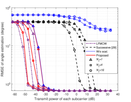
(a) Angle estimation performance

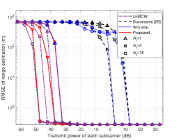
(b) Range estimation performance

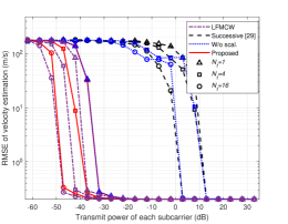
(c) Velocity estimation performance

Figure 3: Estimation performance versus transmit power with different transmit antennas, $N_{\mathrm{t}}=1,4,16$.

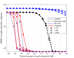
(a) Angle estimation performance

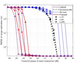
(b) Range estimation performance

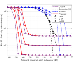
(c) Velocity estimation performance

Figure 4: Estimation performance versus transmit power with different CPI lengths, $L=16,64,256$.

In this section, we provide numerical experiments to verify the advantages of the proposed joint estimation method. It should be emphasized that the estimation method proposed in this paper is dedicated to processing the echoes of MIMO-OFDM waveforms utilized in general communication systems. Therefore, the processing at the communication end is the same as that of conventional communication systems and is ignored in the following simulations. We would also like to emphasize that the proposed estimation method will not cause any communication performance loss since it does not require any modification on the communication MIMO-OFDM waveforms. Unless otherwise specified, we use the settings based on the 3GPP 5G NR high-frequency standard [38], [39], as listed in Table I.

In simulations, we assume that the sensing area of interest is known at the BS. Particularly, potential targets are randomly located within the angle of $-30^{\circ}\sim 30^{\circ}$, the range of $40\mathrm{m}\sim 80\mathrm{m}$, and the velocity of $-50\mathrm{m/s}\sim 50\mathrm{m/s}$. The transmit beamforming matrix is then designed using the typical zero-forcing (ZF) scheme [40] to eliminate the multi-user interference and direct the beams toward both the users and potential targets. In addition to the proposed joint estimation algorithm (denoted as “Proposed”), we also include three counterparts for comparisons. Specifically, to show the significance of maintaining spatial characteristics by introducing the scaling factor $\alpha_{n_{\mathrm{a}}}$, we include the joint estimation algorithm without using scaling when removing the signal-dependent coefficients (denoted as “W/o scal.”). We also present the state-of-the-art algorithm proposed in [29] (denoted as “Successive [29]”), which successively estimates the angle, range, and velocity and only utilizes the echo signals during one OFDM symbol for angle/range estimation. Besides, the pure radar system using a typical LFMCW waveform with the same power budget and bandwidth (denoted as “LFMCW”) is chosen as the benchmark. Particularly, the LFMCW waveform emitted by $N_{\mathrm{t}}$ antennas within one CPI is given as [41]

$$\mathbf{x}_{\mathrm{LFMCW}}(t)\triangleq\mathbf{w}\sum_{l=0}^{L-1}e^{\jmath 2\pi(f_{\mathrm{c}}t+\frac{N_{\mathrm{s}}\Delta f(t-lT)^{2}}{T2})}\mathrm{rect}(\frac{t-lT}{T}),$$ (36)

where $\mathbf{w}\in\mathbb{C}^{N_{\text{t}}\times 1}$ is the precoded vector calculated by ZF scheme [40] with the known interested sensing area, to focus the signals toward interested targets. A typical LFMCW radar receiver with $N_{\mathrm{r}}$ receive antennas and classic 3-dimensional DFT estimation method is employed [41]-[43]. In addition, both the single-target and multi-target scenarios are considered to illustrate the parameter estimation performance. The estimation performance is evaluated in terms of the RMSE of the estimated angle/range/velocity, e.g., the RMSE of the angular estimation is defined as

$$\text{RMSE}\triangleq\sqrt{\mathbb{E}\Big{\{}\frac{1}{Q}\sum_{q=1}^{Q}(\theta_{q}-\widetilde{\theta}_{q})^{2}\Big{\}}},\vspace{-1ex}$$ (37)

where $\theta_{q}$ is the actual DoA and $\widetilde{\theta}_{q}$ is the estimated DoA of the $q$-th target.

V-A Single-Target Scenario

To clearly demonstrate the processing gains achieved by fully exploiting the echo signals during one CPI, in this subsection we consider the single-target scenario. We first show the RMSE of angle/range/velocity estimation versus the transmit power in Fig. 3, in which the schemes with a different number of transmit antennas are included. Not surprisingly, the estimation error of all schemes decreases as the transmit power or the number of transmit antennas increases, since more power or a larger transmit antenna array provides higher-strength echo signals. In addition, we observe that the RMSE of angle/range/velocity estimation tends to be the same constant value with the increasing of $N_{\text{t}}$ and transmit power. This is because the estimation error is lower bounded by the width of each angular/range/Doppler bin, which is irrelevant to the number of transmit antennas and the transmit power. Meanwhile, since the spatial characteristics of echo signals are destroyed when removing the signal-dependent coefficients, the RMSE of angular estimation achieved by the algorithm without scaling is significantly deteriorated in multiple transmit antenna scenarios. Moreover, our proposed joint estimation algorithm greatly outperforms the existing successive estimation algorithm [29], considering that the three-dimensional echo signals are fully exploited to improve the processing gains. Most importantly, by leveraging the proposed estimation algorithm, the sensing performance of using OFDM waveform can get very close to that of a pure radar system using LFMCW waveform without incurring any communication performance loss. This phenomenon confirms the advantages of our proposed joint estimation algorithm and also indicates that OFDM waveform is an attractive candidate for ISAC systems.

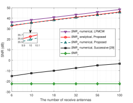
(a) The impact of receive antennas

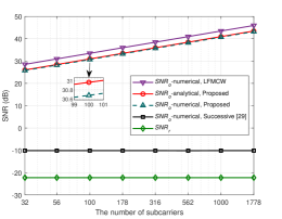
(b) The impact of subcarriers

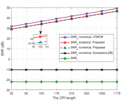
(c) The impact of CPI length

Figure 5: Received and output SNR versus the number of receive antennas, subcarriers, and CPI lengths, respectively.

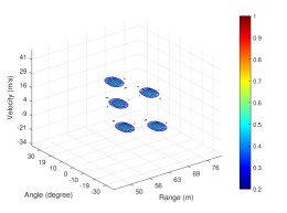
(a) “LFMCW”

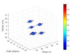
(b) “Proposed”

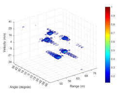
(c) “W/o scal.”

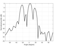
(d) “Successive [29]”

Figure 6: Radar images of different estimation algorithms.

Then, we show the RMSE performance for the schemes with different CPI lengths in Fig. 4. As already noted, by fully utilizing the received echo signals within one CPI and jointly estimating the parameters through three dimensions, the proposed algorithm achieves the lowest RMSE of angle/range/velocity with a given transmit power for tackling MIMO-OFDM waveform echoes and is very close to the LFMCW radar-only scheme. Moreover, compared with the successive estimation algorithm that only utilizes one OFDM symbol for angle/range estimation, the increase of $L$ brings notable performance improvements by using the proposed joint estimation algorithm. In addition, we observe that the RMSE floor of velocity estimation decreases with the increase of $N_{\mathrm{v}}=3L$, which is consistent with the expression of estimated velocity in (24c).

To further quantify the processing gains of the proposed algorithm, in Fig. 5 we illustrate the SNRs of the received echo signals and the output signals after echo signal processing, i.e., $\text{SNR}_{\text{r}}$ in (29) and $\text{SNR}_{\text{o}}$ in (34b), respectively. The SNRs versus the number of receive antennas, the number of subcarriers, and the CPI length, are shown in Figs. 5(a), (b), and (c), respectively. Both the analytical output SNR as expressed in (34b) and the numerical value, which is calculated as the ratio between the power of the peak in $Y(n_{\text{a}},n_{\text{d}},n_{\text{v}})$ and the noise power, are included. It is observed that the numerical results are almost the same as the theoretical values, which verifies the correctness of our theoretical analysis. Moreover, we see that the output SNR of our proposed algorithm linearly increases with the number of receive antennas, the number of subcarriers, and the CPI lengths. This is consistent with the expression of $\text{SNR}_{\text{o}}$ in (34b) and verifies that the proposed joint estimation algorithm can fully exploit the echo signals from three dimensions. In addition, since the performance of the successive estimation algorithm is determined by the angular estimation, we show the output SNR in extracting the angular information, which obviously only increases with the number of receive antennas. These results reveal that the proposed algorithm that fully utilizes the echo signals to jointly extract the angle-range-velocity has substantially higher processing gains compared with its counterpart and comparable to the radar-only LFMCW scheme, e.g., the proposed algorithm achieves a remarkable SNR processing gain of about $50\mathrm{dB}$ merely about $3\mathrm{dB}$ lower than the LFMCW radar, while its counterpart can only provide nearly $10\mathrm{dB}$.

V-B Multi-Target Scenario

In order to illustrate the estimation performance in terms of resolution, in this subsection we consider multi-target scenarios under the noise-free environment. We assume that there exist $Q=5$ point-like targets with the angle-range-velocity parameters listed in Table II.

To visually present the parameter estimation performance, we first show the radar images of different schemes in Fig. 6. We clearly see from Figs. 6(a) and (b) that there are five clusters in the radar image corresponding to the five targets by using the proposed estimation algorithm and the LFMCW radar-only scheme, while the algorithm without scaling in Fig. 6(c) will lead to many wrong peaks along the spatial dimension. Meanwhile, the angle estimation image 6(d) by using the successive estimation algorithm only exhibits three peaks, which indicates that several targets are so close along the spatial dimension that they cannot be distinguished from each other. Thus, there is no doubt that the proposed joint estimation algorithm has better parameter estimation performance. Based on these radar images, we can obtain the estimation results shown in Fig. 7, in which the true values are marked by black circles. Since the algorithm without scaling leads to many wrong peaks, we only show the results by using the proposed joint estimation algorithm, the counterpart of successive estimation, and the LFMCW radar-only strategy. It is obvious that the proposed algorithm provides more accurate estimation results than its counterpart.

TABLE II: Target parameters

Angle	Range	Velocity
$~{}~{}19^{\circ}$	$69\mathrm{m}$	$-30\mathrm{m/s}$
$~{}~{}~{}0^{\circ}$	$70\mathrm{m}$	$~{}~{}10\mathrm{m/s}$
$~{}~{}~{}5^{\circ}$	$60\mathrm{m}$	$~{}~{}25\mathrm{m/s}$
$-25^{\circ}$	$50\mathrm{m}$	$~{}~{}30\mathrm{m/s}$
$-20^{\circ}$	$65\mathrm{m}$	$-5\mathrm{m/s}$

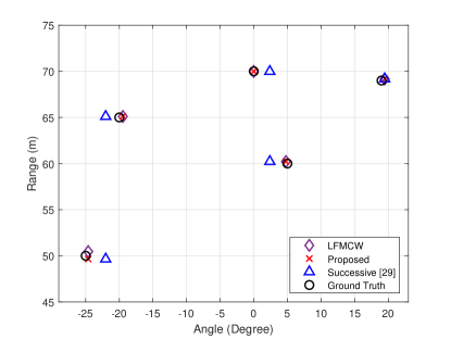
Figure 7: Target estimation results.

Finally, we present the RMSE of angle/range/velocity estimation versus the number of targets in Fig. 8. It is observed that the performance gap between the proposed joint estimation algorithm and the traditional successive estimation algorithm grows with the larger number of targets. This phenomenon indicates that by jointly estimating the angle-range-velocity information, the sensing resolution of targets can be improved and better parameter estimation performance is achieved, especially for scenarios with multiple targets. Moreover, our proposed joint estimation algorithm utilizing MIMO-OFDM communication waveform can achieve nearly the same performance as the LFMCW radar-only scheme.

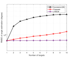
(a) Angle estimation performance

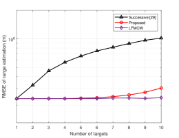
(b) Range estimation performance

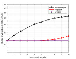
(c) Velocity estimation performance

Figure 8: Estimation performance versus the number of targets.

VI Conclusions

In this paper, we proposed a novel joint estimation algorithm for estimating the parameters of multiple targets based on the conventional MIMO-OFDM communication waveforms in ISAC systems. We jointly estimated the angle-range-velocity information of potential targets by fully exploiting the received echo signals in a coherent processing interval. Theoretical analysis for the maximum unambiguous range, resolution, and processing gain were provided to evaluate the performance of the proposed echo signal processing algorithm. Extensive simulation results verified that the proposed approach can achieve parameter estimation performance much better than the existing algorithm using MIMO-OFDM communication waveform and close to pure radar system using LFMCW waveform. Based on this initial work, we will further investigate transmit beamforming designs and more efficient echo signal processing algorithms for practical applications, in order to achieve a better performance trade-off between multiuser communications and radar target parameter estimation.

References

- [1] ITU-R, DRAFT NEW RECOMMENDATION, “Framework and overall objectives of the future development of IMT for 2030 and beyond,” Jun. 2023.
- [2] L. Zheng, M. Lops, Y. C. Eldar, and X. Wang, “Radar and communication coexistence: An overview: A review of recent methods,” IEEE Signal Process. Mag., vol. 36, no. 5, pp. 85-99, Sep. 2019.
- [3] J. A. Zhang, F. Liu, C. Masouros, R. W. Heath, Z. Feng, L. Zheng, and A. Petropulu, “An overview of signal processing techniques for joint communication and radar sensing,” IEEE J. Sel. Topics Signal Process., vol. 15, no. 6, pp. 1295-1315, Nov. 2021.
- [4] F. Liu, L. Zheng, Y. Cui, C. Masouros, A. Petropulu, H. Griffiths, and Y. C. Eldar, “Seventy years of radar and communications: The road from separation to integration,” IEEE Signal Process. Mag., vol. 40, no. 5, pp. 106-121, Jul. 2023.
- [5] Y. Zhang, Q. Li, L. Huang, and J. Song, “Waveform design for joint radar-communication system with multi-user based on MIMO radar,” in Proc. IEEE Radar Conf. (RadarConf), Seattle, WA, USA, May 2017, pp. 415-418.
- [6] K. Wu, J. A. Zhang, X. Huang, and Y. J. Guo, “Frequency-hopping MIMO radar-based communications: An overview,” IEEE Aerosp. Electron. Syst. Mag., vol. 37, no. 4, pp. 42-54, Apr. 2022.
- [7] G. Han, J. Choi, and R. W. Heath, “Radar imaging based on IEEE 802.11ad waveform in V2I communications,” IEEE Trans. Signal Process., vol. 70, pp. 4981-4996, Oct. 2022.
- [8] M. L. Rahman, J. A. Zhang, X. Huang, Y. J. Guo, and R. W. Heath, “Framework for a perceptive mobile network using joint communication and radar sensing,” IEEE Trans. Aerosp. Electron. Syst., vol. 56, no. 3, pp. 1926-1941, Jun. 2020.
- [9] J. A. Zhang, M. L. Rahman, X. Huang, Y. J. Guo, S. Chen, and R. W. Heath, “Perceptive mobile network: Cellular networks with radio vision via joint communication and radar sensing,” IEEE Veh. Technol. Mag., vol. 16, no. 2, pp. 20-30, Jun. 2021.
- [10] R. Liu, M. Li, Q. Liu, and A. L. Swindlehurst, “Joint waveform and filter designs for STAP-SLP-based MIMO-DFRC systems,” IEEE J. Sel. Areas Commun., vol. 40, no. 6, pp. 1918-1931, Jun. 2022.
- [11] R. Liu, M. Li, Y. Liu, Q. Wu, and Q. Liu, “Joint transmit waveform and passive beamforming design for RIS-aided DFRC systems,” IEEE J. Sel. Topics Signal Process., vol. 16, no. 5, pp. 995-1010, Aug. 2022.
- [12] S. Sen and A. Nehorai, “Adaptive OFDM radar for target detection in multipath scenarios,” IEEE Trans. Signal Process., vol. 59, no. 1, pp. 78-90, Jan. 2011
- [13] S. Sen, “OFDM radar space-time adaptive processing by exploiting spatio-temporal sparsity,” IEEE Trans. Signal Process., vol. 61, no. 1, pp. 118-130, Jan. 2013.
- [14] X. H. Wu, A. A. Kishk, and A. W. Glisson, “MIMO-OFDM radar for direction estimation,” IET Radar Sonar Navig., vol. 4, no. 1, pp. 28-36, Feb. 2010.
- [15] T. Zhang, X.-G. Xia and L. Kong, “IRCI free range reconstruction for SAR imaging with arbitrary length OFDM pulse,” IEEE Trans. Signal Process., vol. 62, no. 18, pp. 4748-4759, Sep. 2014.
- [16] Y.-H. Cao, X.-G. Xia, and S.-H. Wang, “IRCI free colocated MIMO radar based on sufficient cyclic prefix OFDM waveforms,” IEEE Trans. Aerosp. Electron. Syst., vol. 51, no. 3, pp. 2107-2120, Jul. 2015.
- [17] C. Sturm and W. Wiesbeck, “Waveform design and signal processing aspects for fusion of wireless communications and radar sensing,” IEEE Proc., vol. 99, no. 7, pp. 1236-1259, Jul. 2011.
- [18] L. Zheng and X. Wang, “Super-resolution delay-doppler estimation for OFDM passive radar,” IEEE Trans. Signal Process., vol. 65, no. 9, pp. 2197-2210, May 2017.
- [19] Y. Liu, G. Liao, Y. Chen, J. Xu, and Y. Yin, “Super-resolution range and velocity estimations with OFDM integrated radar and communications waveform,” IEEE Trans. Veh. Technol., vol. 69, no. 10, pp. 11659-11672, Oct. 2020.
- [20] J. B. Sanson, P. M. Tomé, D. Castanheira, A. Gameiro, and P. P. Monteiro, “High-resolution delay-doppler estimation using received communication signals for OFDM radar-communication system,” IEEE Trans. Veh. Technol., vol. 69, no. 11, pp. 13112-13123, Nov. 2020.
- [21] Y. Wu, F. Lemic, C. Han, and Z. Chen, “Sensing integrated DFT-Spread OFDM waveform and deep learning-powered receiver design for terahertz integrated sensing and communication systems,” IEEE Trans. Commun., vol. 71, no. 1, pp. 595-610, Jan. 2023.
- [22] Y. Liu, G. Liao, Z. Yang, and J. Xu, “Multiobjective optimal waveform design for OFDM integrated radar and communication systems,” Signal Process., vol. 141, pp. 331-342, Jun. 2017.
- [23] Y. Liu, G. Liao, J. Xu, Z. Yang, and Y. Zhang, “Adaptive OFDM integrated radar and communications waveform design based on information theory,” IEEE Commun. Lett., vol. 21, no. 10, pp. 2174-2177, Oct. 2017.
- [24] M. F. Keskin, V. Koivunen, and H. Wymeersch, “Limited feedforward waveform design for OFDM dual-functional radar-communications,” IEEE Trans. Signal Process., vol. 69, pp. 2955-2970, Apr. 2021.
- [25] J. Li and P. Stoica, “MIMO radar with colocated antennas,” IEEE Signal Process. Mag., vol. 24, no. 5, pp. 106-114, Sep. 2007.
- [26] E. Björnson, Y. C. Eldar, E. G. Larsson, A. Lozano, and H. V. Poor, “Twenty-five years of signal processing advances for multiantenna communications: From theory to mainstream technology,” IEEE Signal Process. Mag., vol. 40, no. 4, pp. 107-117, Jun. 2023.
- [27] Y. Liu, G. Liao, Z. Yang, and J. Xu, “Joint range and angle estimation for an integrated system combining MIMO radar with OFDM communication,” Multidimensional Syst. Signal Process., vol. 30, no. 2, pp. 661-687, 2019.
- [28] M. A. Islam, G. C. Alexandropoulos, and B. Smida, “Integrated sensing and communication with millimeter wave full duplex hybrid beamforming,” in Proc. IEEE Int. Conf. Commun. (ICC), Seoul, Korea, May 2022, pp. 4673-4678.
- [29] Z. Xu and A. Petropulu, “A bandwidth efficient dual-function radar communication system based on a MIMO radar using OFDM waveforms,” IEEE Trans. Signal Process., vol. 71, pp. 401-416, Feb. 2023.
- [30] M. Bernhardt, F. Gregorio, J. Cousseau, and T. Riihonen, “Self-interference cancelation through advanced sampling,” IEEE Trans. Signal Process., vol. 66, no. 7, pp. 1721-1733, Apr. 2018.
- [31] C. B. Barneto, S. D. Liyanaarachchi, M. Heino, T. Riihonen, and M. Valkama, “Full duplex radio/radar technology: The enabler for advanced joint communication and sensing,” IEEE Wireless Commun., vol. 28, no. 1, pp. 82-88, 2021.
- [32] G. C. Alexandropoulos, M. A. Islam, and B. Smida, “Full-duplex massive multiple-input, multiple-output architectures: Recent advances, applications, and future directions,” IEEE Veh. Technol. Mag., vol. 17, no. 4, pp. 83-91, Dec. 2022.
- [33] J. G. Proakis, “The discrete Fourier transform: Its properties and applications,” Digital Signal Processing: Principles, Algorithms and Applications, 4th ed. Upper Saddle River, N.J.: Pearson Education, 2007, pp. 449-502.
- [34] R. O. Schmidt, “Multiple emitter location and signal parameter estimation,” IEEE Trans. Antennas Propagat., vol. 34, pp. 276-280, Mar. 1986.
- [35] R. Roy and T. Kailath, “ESPRIT-estimation of signal parameters via rotational invariance techniques,” IEEE Trans. Acoust., Speech, Signal Process., vol. 37, no. 7, pp. 984-995, Jul. 1989.
- [36] M. Braun, C. Sturm, and F. K. Jondral, “On the single-target accuracy of OFDM radar algorithms,” in Proc. IEEE 22nd Int. Symp. Pers., Indoor Mobile Radio Commun., Toronto, Canada, 2011, pp. 794-798.
- [37] M. Braun, “OFDM radar algorithms in mobile communication networks,” Ph.D. dissertation, Dept. Inst. Commun. Eng., Karlsruher Instituts fur Technologie, Karlsruhe, Germany, 2014.
- [38] 3GPP, “3GPP TS 38.104 V17.8.0 (2022-12) 3rd Generation Partnership Project; Technical Specification Group Radio Access Network; NR; Base Station (BS) radio transmission and reception (Release 17),” 2022.
- [39] 3GPP, “3GPP TS 38.211 V17.4.0 (2022-12) 3rd Generation Partnership Project; Technical Specification Group Radio Access Network; NR; Physical channels and modulation (Release 17),” 2022.
- [40] Q. H. Spencer, A. L. Swindlehurst, and M. Haardt, “Zero-forcing methods for downlink spatial multiplexing in multiuser MIMO channels,” IEEE Trans. Signal Process., vol. 52, no. 2, pp. 461-471, Feb. 2004.
- [41] M. Jankiraman, FMCW Radar Design. Norwood, MA, USA: Artech House, 2008.
- [42] S. Saponara and B. Neri, “Radar sensor signal acquisition and multidimensional FFT processing for surveillance applications in transport systems,” IEEE Trans. Instrum. Meas., vol. 66, no. 4, pp. 604-615, Apr. 2017.
- [43] X. Li, X. Wang, Q. Yang, and S. Fu, “Signal processing for TDM MIMO FMCW millimeter-wave radar sensors,” IEEE Access, vol. 9, pp. 167959-167971, Dec. 2021.