Counterfactual Monotonic Knowledge Tracing for Assessing Students’ Dynamic Mastery of Knowledge Concepts

Abstract.

As the core of the Knowledge Tracking (KT) task, assessing students’ dynamic mastery of knowledge concepts is crucial for both offline teaching and online educational applications. Since students’ mastery of knowledge concepts is often unlabeled, existing KT methods rely on the implicit paradigm of historical practice $\rightarrow$ mastery of knowledge concepts $\rightarrow$ students’ responses to practices to address the challenge of unlabeled concept mastery. However, purely predicting student responses without imposing specific constraints on hidden concept mastery values does not guarantee the accuracy of these intermediate values as concept mastery values. To address this issue, we propose a principled approach called Counterfactual Monotonic Knowledge Tracing (CMKT), which builds on the implicit paradigm described above by using a counterfactual assumption to constrain the evolution of students’ mastery of knowledge concepts. Specifically, CMKT first assesses students’ knowledge concept mastery value based on their historical practice sequences. Then, CMKT sets the answer of the most recent practice as the opposite of the actual answer and, based on this counterfactual answer, assesses the student’s corresponding counterfactual knowledge mastery value. During the model training process, CMKT constrains the update of the student’s knowledge states by ensuring that the two types of knowledge mastery values of students satisfy a fundamental educational theory, the monotonicity theory, to provide specific semantics for the assessed mastery values by the model. Moreover, we predict the student’s responses to practices by directly measuring the difference between the student’s knowledge concept mastery value and the difficulty of the target question, using labels of students’ responses to assist model training. Finally, we conduct extensive experiments on five real-world datasets to demonstrate the superiority of CMKT over multiple baseline models. The code is available at https://github.com/zmy-9/CMKT.

1. Introduction

Currently, there are two essential research tasks in online education: the Cognitive Diagnosis (CD) task (cd_task1, ; cd_task2, ; irt, ) and the Knowledge Tracing (KT) task (kt_task, ; bkt1, ; bkt2, ; kt_survey2, ; kt_survey3, ). Although both tasks aim to track students’ knowledge states based on their historical practice behavior, there are some distinctions between them. The CD task assumes that students’ knowledge state is static and typically assesses their knowledge mastery in a testing environment (e.g., an exam), as depicted in Figure 1(a). In contrast, the KT task traces the dynamic changes in students’ knowledge level and is generally employed for long-term student learning assessment, as shown in Figure 1(b). Assessing students’ mastery of knowledge concepts in the KT task is more arduous than in the CD task because students’ knowledge mastery evolves dynamically (learning_efficiency1, ; learning_efficiency2, ). Nevertheless, we endeavor to improve existing KT methods in assessing students’ knowledge mastery, as evaluating students’ evolving mastery of knowledge concepts can be of significant practical value in aiding online platforms to furnish understandable feedback and suitable learning materials to students (kt_task, ; kt_survey, ; provide_materials, ). For instance, by utilizing the assessed mastery values of knowledge concepts, we can generate personalized learning paths for students based on the educational knowledge graph on the online learning platform (learn_path1, ; learn_path2, ; pre_relation1, ; pre_relation2, ).

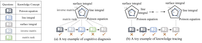
Figure 1. Examples of the cognitive diagnosis (CD) task and the knowledge tracing (KT) task.

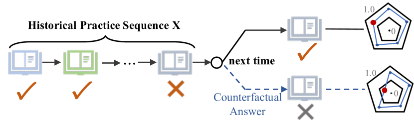
Figure 2. Illustration of the counterfactual assumption.

However, due to the lack of labels of students’ mastery of knowledge concepts, both CD and KT tasks adopt the implicit paradigm of historical practices $\rightarrow$ mastery of knowledge concepts $\rightarrow$ students’ responses to practices to optimize the model’s parameters, where the labels of students’ responses are binary values indicating whether the student answered the question correctly. The initial motivation for this paradigm is reasonable, as students who have a higher master level of knowledge concepts are more likely to correctly answer questions than those who have a lower mastery level. However, in recent years, deep neural networks have been increasingly employed in KT models to enhance the accuracy in predicting students’ responses (dkt, ; akt, ; sakt, ; mf_dakt, ), resulting in black-box properties of the models that make it challenging to ensure that the intermediate values in the model still reflect the students’ mastery of concepts, thereby lacking interpretability and semantic information.

To more accurately track students’ comprehension of concepts, Learning Process-consistent Knowledge Tracing (LPKT) (lpkt, ) proposes to maintain consistency in the learning process by measuring learning gains based on the difference between current and past practices. However, LPKT only focuses on the positivity of the learning gain for each practice and fails to explicitly model the relationship between the relative size of learning gains for different practices. Consequently, LPKT cannot guarantee that the assessed mastery value of knowledge concepts satisfies the monotonicity theory (monotonicity1, ), which presumes that a student’s mastery of a knowledge concept and the probability of incorrectly answering questions related to the concept is monotonous. There is a CD model called IRR (irr, ), proposes using a pairwise training method to directly incorporate this monotonicity during model training. However, the monotonicity design of IRR remains at the question granularity, rather than imposing monotonic constraints on the mastery of knowledge concepts. In fact, if we could directly constrain these mastery values to adhere to the monotonicity theory, we could give the assessed mastery values stronger interpretability and semantic information. However, applying the monotonicity theory directly to knowledge concept granularity is challenging, as we cannot be certain that a student who correctly answers a question involving multiple concepts has a higher mastery of each concept than a student who answers incorrectly, as the latter may only have a poor mastery level of a specific knowledge concept, not every concept. Consequently, imposing reasonable constraints on knowledge mastery values remains a significant challenge.

To address the above challenge, we propose a hypothesis: If a student’s answer to the question answered in the previous practice are opposite to the true answer, what would be the difference between his knowledge mastery value and the mastery value of the real situation? Leveraging this counterfactual hypothesis, we propose a new model named Counterfactual Monotonic Knowledge Tracing (CMKT) to enhance the interpretability and rationality of assessing students’ mastery of knowledge concepts.

Specifically, as previously mentioned, the KT task requires modeling the update of students’ knowledge state throughout the practice process, based on their historical practice sequences. Thus, CMKT devises a knowledge extraction module to model the student’s practice sequence as their knowledge state, which is then mapped to the student’s mastery value for each concept. Due to the lack of labels for students’ knowledge mastery values, we employ the aforementioned implicit KT paradigm to train model parameter by predicting students’ responses to practices. To ensure the knowledge mastery value’s interpretability, we predict the student’s response by directly comparing the relative size between the student’s knowledge mastery value and the difficulty of the question based on the traditional CD method named Item Response Theory (IRT) (irt, ; akt, ). However, this method still optimizes the model at the question level, which does not guarantee that the mastery value of the specific concept satisfies the monotonicity theory.

Considering that merely relying on predicting students’ responses to practices does not ensure that the intermediate values of the model represent knowledge mastery values, we further propose a counterfactual monotonicity constraint during model training, as depicted in Figure 2. Specifically, given a student’s historical practice sequence, we can assess his mastery of concepts using KT models. However, if we assume that his most recent practice answer was the opposite of the true answer, assessed knowledge mastery value by the model in this counterfactual situation should differ from that assessed in the actual situation. For example, if the student’s actual answer is correct, but we assume it is wrong, then based on the monotonicity theory, the mastery value of the relevant concepts in the counterfactual situation assessed by the model should not surpass the corresponding knowledge mastery value of the actual situation, and vice versa. Based on this counterfactual monotonicity assumption, CMKT constructs a counterfactual sample for each training sample during model training and generates sample pairs based on the counterfactual monotonicity for pairwise training, to constrain the concept mastery value in the model evaluation adhering to the monotonicity theory.

In addition, to evaluate the performance of KT methods in assessing students’ dynamic mastery value of concepts directly and effectively, we propose a new metric called Group AUC of Mastery (GAUCM) based on the monotonicity theory. Finally, we employ the GAUCM metric along with two commonly used metrics for predicting students’ responses to demonstrate the superior performance of CMKT compared to multiple baselines. In summary, the main contributions of this paper are as follows:

• To the best of our knowledge, we are the first KT study to propose counterfactual monotonicity. Our innovative approach combines counterfactual inferences with the monotonicity theory to explicitly constrain students’ knowledge mastery at the knowledge concept level, making the mastery value update process more semantically informative and interpretable.

• We define a structure to map students’ historical practice sequences to their mastery values for each knowledge concept, and explicitly model the relationship between students’ mastery values for knowledge concepts and their practice responses.

• We conduct extensive experiments on five real-world KT datasets to validate the superiority of CMKT over state-of-the-art methods in assessing the value of students’ mastery of knowledge concepts based on multiple metrics.

2. Related Work

Current knowledge tracing (KT) methods can be divided into traditional methods and deep learning-based methods, where traditional types include Bayesian methods and factors-based methods. The most representative Bayesian method is Bayesian Knowledge Tracing (BKT) (bkt1, ; bkt2, ), which describes the knowledge state with a binary variable based on the Hidden Markova Model (HMM). The other line is the factor analysis method, where Item Response Theory (IRT) (irt, ) is one of the most classical methods. IRT aims to model the relationship between students’ ability and responses by measuring the gap between their ability and question difficulty, which has been applied in lots of CD models (dirt, ; neuralcdm, ; cdmfkc, ; kscd, ), and KT models. Later, Multidimensional IRT (MIRT) (mirt, ) extends the parameters in IRT into multidimensional space. However, these methods ignore that the students’ learning process is dynamic. Later, many models extended IRT by introducing students’ practical behavior and many auxiliary information, such as AFM (afm, ) and PFA (pfa, ) record the number of students’ practice to introduce practice information, DAS3H (das3h, ) and Knowledge Tracing Machine (KTM) (ktm, ) model introduce Factorization Machine (FM) (fm, ) to construct a generalization framework that introduces richer features. MF-DAKT (mf_dakt, ) introduces the deep neural network to further enhance the modeling capabilities of traditional methods. However, while these methods improve the predictive performance of the model, the interpretability of the model is also gradually weakened.

In recent years, with the development of deep learning, most KT research mainly focuses on deep methods (sakt, ; akt, ). Deep Knowledge Tracing (DKT) (dkt, ) firstly applies the LSTM (lstm, ) into the KT task. Later, the Memory-Augmented Neural Network (MANN) (mann, ), the Transformer structure (transformer, ), the Convolutional Neural Network (CNN) (cnn, ), the Hawkes process (hawkes, ) and other advanced network structures were introduced into the KT task to enhance the ability to predict students’ responses to practices (dkvmn, ; sakt, ; akt, ; hawkeskt, ; ckt, ; iekt, ; dimkt, ; lfbkt, ). To obtain students’ concept mastery values, Dynamic Key-Value Memory model (DKVMN) (dkvmn, ) utilizes a matrix to store students’ dynamic mastery of concepts based on the MANN. Later, Graph-based KT method (GKT) (gkt, ) and Structure-based KT method (SKT) (skt, ) enhances DKT by exploiting the graph structure of concepts and directly models the students’ mastery of each concept. Convolutional Knowledge Tracing method (CKT) (ckt, ) applies the CNN to output a matrix representing students’ mastery of concepts. Learning Process-consistent method (LPKT) (lpkt, ) further proposes to focus on the evolution of students’ states during the learning process by maintaining consistency of students’ changing knowledge state. However, although these methods also try to obtain students’ concept mastery values, they generally represent the students’ mastery of a concept in the form of vectors, and do not generate a mastery value during model optimization, making it difficult to ensure that these values conform to the monotonicity theory. Therefore, in this paper, we propose the Counterfactual Monotonic Knowledge Tracing model to address the above issues.

3. Preliminary

In this section, we formally define the task of assessing students’ mastery of concepts and briefly introduce the terminologies and the counterfactual monotonicity constraints proposed in this paper.

3.1. Problem Statement

For student $s$ at time $t$, we can observe his time-ordered answer history behavior before time t, denoted as $X=\left\{(q_{1},a_{1}),...,(q_{t},a_{t})\right\}$, where $a_{t}\in\left\{0,1\right\}$ indicates whether $s$ answered question $q_{t}$ correctly. As a question may involve multiple knowledge concepts, we denote the concept set of $q_{t}$ as $K_{q_{t}}$. The embedding vectors for question $q_{t}$ and concept $k_{j}$ are denoted as $\boldsymbol{q}_{i}\in\mathbb{R}^{d_{q}}$ and $\boldsymbol{k}_{j}\in\mathbb{R}^{d_{k}}$, respectively, where $d_{q}$ and $d_{k}$ denote the dimensionality of vectors.

Previous studies have highlighted the impact of question difficulty on student learning since correctly answering more challenging questions may significantly impact their knowledge states (dimkt, ; mf_dakt, ). Thus, we incorporate difficulty information into our model to model the learning process of students. Typically, the lower the correct answer rate, the more difficult the question is perceived by students. Based on this, we define the difficulty of a question as the ratio of incorrect answers to that question in the dataset, denoted as $\theta_{q}\in[0,1]$. To create a sparse difficulty level feature, we multiply $\theta_{q}$ by a constant $C_{q}$ and round it, and then embed it as $\boldsymbol{\theta}_{q}\in\mathbb{R}^{d_{q{\theta}}}$ in a $d_{q{\theta}}$-dimensional vector. Similarly, we compute the average difficulty level for each knowledge concept across all questions, denoted as $\theta_{k}\in[0,1]$ and use the constant $C_{k}$ to embed $\theta_{k}$ as $\boldsymbol{\theta}_{k}\in\mathbb{R}^{d_{k{\theta}}}$, where $d_{k{\theta}}$ is the dimension of the vector.

In this way, the practice record occurring at time $t$ can be formed as $p_{t}=(a_{t},q_{t},\theta_{q_{t}},\left\{k_{i}\right\}_{k_{i}\in K_{q_{t}}},\left\{\theta_{k_{i}}\right\}_{k_{i}\in K_{q_{t}}})$. We characterize this practice behavior by combining the raw embedding vectors of the input features. The specific calculation formula is as follows:

(1) $$\boldsymbol{p}_{t}=\boldsymbol{W}_{1}^{T}[\boldsymbol{a_{t}}\oplus\boldsymbol{q_{t}}\oplus\boldsymbol{\theta}_{q_{t}}\oplus\sum_{k_{i}\in K_{q_{t}}}(\boldsymbol{W}_{0}^{T}(\boldsymbol{k}_{i}\oplus\boldsymbol{\theta}_{k_{i}})+\boldsymbol{b}_{0})]+\boldsymbol{b}_{1}^{T}$$

where $\boldsymbol{a_{t}}\in\mathbb{R}^{d_{a}}$ is the embedding of $a_{t}$. $\oplus$ is the concatenation operation. $\boldsymbol{W}_{0}^{T}(\boldsymbol{k}_{i}\oplus\boldsymbol{\theta}_{k_{i}})+\boldsymbol{b}_{0}$ denotes the combination of embedding of each concept in $K_{q_{t}}$ and corresponding concept difficulty. $\boldsymbol{W}_{0}\in\mathbb{R}^{(d_{k}+d_{k{\theta}})\times d}$, $\boldsymbol{W}_{1}\in\mathbb{R}^{(d_{a}+d_{q}+d_{q{\theta}}+d)\times d}$ are the weight matrices, $\boldsymbol{b}_{0}$, $\boldsymbol{b}_{1}\in\mathbb{R}^{d}$ are the bias terms. $d$ is the dimension of vectors.

Task Definition. Given a student’s historical practice sequence $X$ before time $t$, we aim to assess the student’s mastery value of knowledge concepts after this period of practice, denoted as $\boldsymbol{M}_{t}=\left\{m_{t1},...,m_{ti},...,m_{tN_{k}}\right\}$. $N_{k}$ denotes the total number of knowledge concepts in the dataset. Here, $m_{ti}$ represents the student’s mastery of knowledge concept $k_{i}$ at time t. As we cannot obtain labeled data on a student’s mastery of a concept, we introduce the label of the student’s responses to practices as a training objective and optimize the model parameters by predicting the student’s future performance at the next time step $t+1$. Meanwhile, in this process, we hope that the student’s knowledge mastery values of concepts, which are implicit intermediate values of the model, retain the property of knowledge mastery value.

3.2. Terminology Definition

To facilitate understanding of the process of assessing mastery of concepts in this paper, we first define the following terminologies:

Definition 3.1. (Students’ Knowledge States). As students practice over time, their knowledge state changes as they receive learning gains with each practice. The knowledge states not only reflect their mastery of knowledge concepts at each moment, but also affect their subsequent performance. By modeling a student’s historical practice sequence before time $t$ chronologically, we can obtain his knowledge state denoted as $\boldsymbol{h}_{t}=\boldsymbol{F}_{ke}(p_{1},p_{2},...,p_{t})$, where $\boldsymbol{h}_{t}\in\mathbb{R}^{d}$ and $d$ is the dimension of this hidden vector. $\boldsymbol{F}_{ke}$ represents a function that models knowledge state updates in a student’s practice sequence, e.g., $\boldsymbol{F}_{ke}$ is the LSTM in the DKT model (dkt, ).

Definition 3.2. (Students’ Mastery of Concepts). Typically, KT studies set a student’s mastery of a target concept on a scale of 0 to 1, where values closer to 1 denote greater levels of knowledge mastery (dkvmn, ; dkt, ; lpkt, ; dkt, ; ckt, ; akt, ). When a student attains a mastery value of 1 for a concept, he can be deemed to have fully mastered that concept. Assuming that a question pertains to only one knowledge concept, it can be inferred that students should be able to answer any related question correctly. And if a student can correctly answer the most challenging questions related to a particular concept, he can correctly answer all other related questions. Therefore, a student’s mastery of a concept can be considered as the probability of accurately answering the most difficult practices related to that concept. To represent practices that involve the highest difficulty level of the target concept, we combine the embedding of the concept with the embedding of the highest difficulty level. We then calculate a student’s mastery of concept $k_{i}$ at time $t$ as $m_{ti}=P(a=1|\boldsymbol{h}_{t},k_{i},C_{k})$, where $C_{k}$ denotes the highest difficulty level of concepts.

3.3. Counterfactual Monotonicity

As previously mentioned, KT methods assess students’ mastery of concepts by predicting their responses to practices, but these mastery values lack specific semantics due to the lack of direct constraints. We believe that the primary issue is the failure to make the mastery value conform to some fundamental educational theories, such as the monotonicity theory (monotonicity1, ). The theory asserts that students who answer a question correctly have a higher degree of mastery of concepts related to that question than students who answer incorrectly. Based on this, IRR (irr, ) employed pairwise training loss to introduce the monotonicity into model training. However, the above monotonicity theory only works at the granularity of the question. For questions involving multiple knowledge concepts, students who answer the question correctly may not necessarily have a higher degree of mastery of each knowledge concept related to the question than students who answer incorrectly. A student may not possess a high level of mastery of a particular knowledge concept, resulting in an incorrect answer, but still display a high degree of mastery of other knowledge concepts. Therefore, faced with this complex student learning situation, achieving monotonic constraints at the granularity of concepts poses a challenge for us.

Since there are no labels for students’ mastery of knowledge concept, it is challenging to verify whether concept-level mastery values vary monotonically based on existing samples. However, inspired by counterfactual learning (counterfactual1, ; counterfactual2, ), we propose that a monotonicity theory based on the counterfactual assumption. For instance, if a student answers a question $q$ related to two concepts $k_{1}$ and $k_{2}$ correctly, we denote that his mastery value for $k_{1}$ and $k_{2}$ after answering $q$ are $m_{1}$ and $m_{2}$, respectively. We then pose a counterfactual question: If he answers $q$ incorrectly, how would his mastery values for the two knowledge concepts change? Although we cannot determine the exact learning gain for answering $q$ correctly, we know that the state corresponding to a correct answer should have a higher mastery value than the value after an incorrect answer. Therefore, we assume that the mastery values after incorrect answers are $\overline{m}_{1}$ and $\overline{m}_{2}$, respectively. Instead of using uncertainty counterfactual inference, we can establish a simple and explicit counterfactual monotonic relationship: $m_{1}\geq\overline{m}_{1}$ and $m_{2}\geq\overline{m}_{2}$. Based on this counterfactual monotonic relationship, we can develop training objectives to help the model directly constrain the evolution of knowledge mastery during training, thereby obtaining more accurate and semantically meaningful mastery values.

4. Method

In this section, we provide details about the CMKT model. The primary structure of CMKT is shown in Figure 3. Specifically, CMKT employs a knowledge extraction module to model the evolution of students’ knowledge states during practice. Then, based on Definition 3.2, CMKT maps the hidden vectors that represent the knowledge states to their mastery values for each knowledge concept. We introduce a counterfactual monotonicity constrained regularization term to restrict the update process of students’ mastery values of knowledge concepts, providing rich semantic information and enhancing the accuracy of the assessed mastery values by ensuring that knowledge mastery values satisfy counterfactual monotonicity. Moreover, to improve interpretability, we predict students’ answers to questions based on the relative size between their knowledge mastery and the difficulty of the question, and then jointly optimize model parameters with a loss function for predicting student responses and the counterfactual monotonicity constraint term.

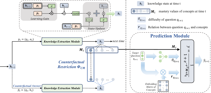
Figure 3. The architecture of the Counterfactual Monotonic Knowledge Tracing model (CMKT).

4.1. Knowledge Extraction

As a student’s knowledge state changes with practice, we must update their knowledge states according to the sequence of their practice behaviors. Since each practice covers different questions with varying difficulty levels, the learning gains also differ. Therefore, we model the learning gains brought by each practice and update the knowledge states accordingly. The process is as follows:

Learning Gain. Students possess varying prior knowledge states, which can be seen as their learning abilities (ckt, ). Consequently, even when practicing the same question, students may experience different learning gains based on different prior knowledge states. Similar to previous works DIMKT (dimkt, ) and LFBKT (lfbkt, ), we propose to model the learning gain of the practice $p_{t}$ using both the prior knowledge state and current practice-related features as:

(2) $$\boldsymbol{z}_{t}=\sigma(\boldsymbol{W}_{2}^{T}(\boldsymbol{h}_{t-1}\oplus\boldsymbol{p}_{t})+\boldsymbol{b}_{2})$$

(3) $$\boldsymbol{l}_{t}=\boldsymbol{z}_{t}\odot\boldsymbol{p}_{t}$$

(4) $$\boldsymbol{\widetilde{h}}_{t}=tanh(\boldsymbol{W}_{3}^{T}(\boldsymbol{h}_{t-1}\oplus\boldsymbol{l}_{t})+\boldsymbol{b}_{3})$$

where $\sigma$ denotes the sigmoid function. $\odot$ denotes the element-wise product. $\boldsymbol{z}_{t}\in\mathbb{R}^{d}$ is the student’s personalized perception of this practice under the prior knowledge state $\boldsymbol{h}_{t-1}$. $\boldsymbol{l}_{t}\in\mathbb{R}^{d}$ represents the unique learning gain brought by $p_{t}$ under the prior knowledge state. Learning gain representations. We then can obtain the student’s updated knowledge acquisition as $\boldsymbol{\widetilde{h}}_{t}\in\mathbb{R}^{d}$. $\boldsymbol{W}_{2}$, $\boldsymbol{W}_{3}\in\mathbb{R}^{2d\times d}$ are the weight matrices, and $\boldsymbol{b}_{2}$, $\boldsymbol{b}_{3}\in\mathbb{R}^{d}$ are the bias terms.

State Updating. As students learn from practices, they may forget knowledge from the previous knowledge state due to the forgetting behavior that is closely related to both their current exercises and prior knowledge state (dkt, ; das3h, ). Thus, we need to model the forgetting rate at this moment in order to update their knowledge state:

(5) $$\boldsymbol{f}_{t}=\sigma(\boldsymbol{W}_{4}^{T}(\boldsymbol{h}_{t-1}\oplus\boldsymbol{p}_{t})+\boldsymbol{b}_{4})$$

(6) $$\boldsymbol{h}_{t}=\boldsymbol{f}_{t}\odot\boldsymbol{h}_{t-1}+(\mathbf{1}-\boldsymbol{f}_{t})\odot\boldsymbol{\widetilde{h}}_{t}$$

where $\boldsymbol{h}_{t}$ denotes the updated knowledge state at time step $t$. $\boldsymbol{W}_{4}\in\mathbb{R}^{2d\times d}$ is the weight matrix, and $\boldsymbol{b}_{4}\in\mathbb{R}^{d}$ is the bias term.

4.2. Assess Students’ Mastery of Concepts

After obtaining a student’s knowledge state, CMKT needs to map this hidden vector $\boldsymbol{h}_{t}$ to the mastery values of each knowledge concept. Based on Definition 3.2, a student’s mastery of a target concept can be defined as the probability of correctly answering the question that involves that concept with the highest difficult level. Therefore, we propose to combine the target concept embedding with the embedding corresponding to the highest difficulty level of concepts to represent a virtual question, which can then be used to measure a student’s mastery of the concept, as follows:

(7) $$\boldsymbol{\widetilde{q}}_{k_{i}}=tanh(\boldsymbol{W}_{5}^{T}(\boldsymbol{k}_{i}\oplus\boldsymbol{\theta}_{C_{{\theta}k}})+\boldsymbol{b}_{5})$$

where $\widetilde{q}_{k_{i}}$ denotes the virtual question which involves $k_{i}$ with the highest difficult level. $\boldsymbol{W}_{5}\in\mathbb{R}^{(d_{k}+d_{{\theta}k})\times d}$ is the weight matrix, and $\boldsymbol{b}_{5}\in\mathbb{R}^{d}$ is the bias term. At this time, due to that $\boldsymbol{\widetilde{q}}_{k_{i}}$ contains the highest difficulty level of $k_{i}$, a student can be seen as a higher probability of fully master concept $k_{i}$ when he has a higher probability correctly answering $\boldsymbol{\widetilde{q}}_{k_{i}}$. Then, we can calculate the students’ mastery of concept $k_{i}$ based on $\boldsymbol{\widetilde{q}}_{k_{i}}$, i.e., $m_{ti}$, as follows:

(8) $$m_{ti}=\sigma(\boldsymbol{W}_{5}^{T}(\boldsymbol{\widetilde{q}}_{k_{i}}\oplus\boldsymbol{h}_{t}))$$

$\boldsymbol{W}_{5}\in\mathbb{R}^{2d\times 1}$ is the weight matrix used to predict the probability of correctly answering the virtual question based on the current knowledge state. In this way, we can obtain the student’s mastery values of $K$ concepts at time $t$ as $\boldsymbol{M}_{t}=\left\{m_{t1},...,m_{ti},...,m_{tK}\right\}$.

4.3. Counterfactual Monotonicity Restriction

Although there are some methods that have attempted to introduce monotonicity theory or impose constraints to regulate students’ knowledge mastery mastery (irr, ; lpkt, ), none of them can enforce monotonic constraints at the knowledge concept granularity level for students’ mastery of concepts. To bridge this gap, we use the counterfactual monotonicity theory proposed in Section 3.3 to directly constrain the mastery of each knowledge concept. Specifically, suppose a student’s knowledge mastery level at a certain point is $M$, and his most recent practice was to answer question $q$ with the answer $A$. In the KT task, we can observe only one of two potential knowledge mastery outcomes for each student practice, depending on the student’s response to question $q$ during that practice. If $A=a$, where $a$ denotes the real answer, we can observe a mastery level of $M=\boldsymbol{M}_{A=a}$. If $A=1-a$, we can infer a counterfactual result of $M=\boldsymbol{M}_{A=1-a}$. At this point, we need to learn the following functions:

(9) $$\begin{aligned} &\mathbb{E}[\boldsymbol{M}_{A=a}-\boldsymbol{M}_{A=1-a}|\boldsymbol{h},q,A]\\ =&\mathbb{E}[\boldsymbol{M}_{A=a}|\boldsymbol{h},q,A]-\mathbb{E}[\boldsymbol{M}_{A=1-a}|\boldsymbol{h},q,A]\end{aligned}$$

where $\boldsymbol{h}$ denote the student’s knowledge state before answering $q$. According to the counterfactual monotonicity, we can deduce that if $a=1$, then $\mathbb{E}[\boldsymbol{M}_{A=a}-\boldsymbol{M}_{A=1-a}|A,q]\geq 0$, otherwise $\leq 0$. The above formula can be interpreted as follows: Given a student’s previous knowledge state $\boldsymbol{h}$ indicating the ability to correctly answer the next question $q$, and assuming the true answer $a$ is also 1, the student’s knowledge level may remain the same or slightly improve. However, if we suppose that the student answered $q$ incorrectly, it can be inferred that the student has forgotten some knowledge, resulting in a decline in his mastery of concepts related to $q$. Thus, based on this counterfactual answer, the student’s knowledge mastery value of concepts related to $q$ should be lower than the mastery value from the true answer. By applying the counterfactual constraint, we can rationalize the process of updating students’ understanding of concepts. Specifically, for the practice $p_{t}$ that occurred at the previous time $t$, we can construct counterfactual samples as follows:

(10) $$\boldsymbol{\overline{p}}_{t}=\boldsymbol{W}_{1}^{T}[\boldsymbol{q_{t}}\oplus\theta_{q_{t}}\oplus\sum_{k_{i}\in K_{q_{t}}}(\boldsymbol{W}_{0}^{T}(\boldsymbol{k}_{i}\oplus\boldsymbol{\theta}_{k_{i}})+\boldsymbol{b}_{0})\oplus\boldsymbol{\overline{a}}_{t}]+\boldsymbol{b}_{1}^{T}$$

where $\boldsymbol{\overline{a}}_{t}$ denotes the embedding of the counterfactual answer $\overline{a}_{t}$, and $\overline{a}_{t}=1-a_{t}$. After that, we can obtain the student’s counterfactual mastery of concept $k_{i}$, i.e., $\overline{m}_{ti}$, as follows:

(11) $$\boldsymbol{\overline{h}}_{t}=\boldsymbol{F}_{ke}(\boldsymbol{h_{t-1}},\boldsymbol{\overline{p}}_{t})$$

(12) $$\overline{m}_{ti}=m_{ti,\,A=1-a_{t}}=\sigma(\boldsymbol{W}_{5}^{T}(\boldsymbol{\widetilde{q}}_{k_{i}}\oplus\boldsymbol{\overline{h}}_{t}))$$

where $\boldsymbol{F}_{ke}(\cdot)$ denotes the knowledge extraction module. We then set restrictions to regularize the evolution of mastery of concepts (hinge1, ; hinge2, ), as shown by the following formula:

(13) $$\begin{aligned} \Phi_{CM}&=\begin{cases}\mathbb{E}[\boldsymbol{M}_{A=a}-\boldsymbol{M}_{A=1-a}\,|\,A\,]\geq 0,\quad a=1\\ \mathbb{E}[\boldsymbol{M}_{A=a}-\boldsymbol{M}_{A=1-a}\,|\,A\,]\leq 0,\quad a=0\end{cases}\\ &=\sum_{t=1}^{T}\sum_{k_{i}\in K_{e_{t}}}(\frac{1}{\mu}\max[0,1-(m_{ti}-\overline{m}_{ti})(a_{t}-\overline{a}_{t})]^{2})\end{aligned}$$

where $\mu$ is a smoothing parameter which can be artificially adjusted. The square operation is designed to prevent non-differentiability.

4.4. Predict Students’ Responses

To incorporate students’ response labels into model training, we predict students’ responses based on the difference between their knowledge mastery values and the difficulty levels of the target questions based on MIRT (mirt, ). The process is illustrated below:

(14) $$\hat{y}=\frac{1}{1+e^{-\boldsymbol{r}_{q}{\boldsymbol{M}}+\theta_{q}}}$$

where $\boldsymbol{r}_{q}\in\mathbb{R}^{K}$ can be seen as the relationship between question $q$ and $K$ knowledge concepts. $\boldsymbol{M}$ denotes the student’s mastery values of $K$ concepts. $\theta_{q}$ denotes the difficulty of question $q$. However, considering that the question difficulty in Section 3.1 is obtained by statistics from the dataset, this method may introduce noise when the question occurs less frequently. Therefore, as previous studies did (mf_dakt, ), we introduce a fully-connected layer to map the embedding vector of the question to the difficulty value, making it immune to the noise of statistical features:

(15) $$\widetilde{\theta}_{q_{t+1}}=\sigma(\boldsymbol{W}_{6}^{T}\boldsymbol{q}_{t+1}+\boldsymbol{b}_{6})$$

where $\widetilde{\theta}_{q_{t+1}}$ denotes the estimated difficulty of question $q_{t+1}$ by our model. $\boldsymbol{W}_{6}\in\mathbb{R}^{d\times 1}$ and $\boldsymbol{b}_{6}\in\mathbb{R}^{1}$ are parameters to learn.

In reality, when answering a target question, students do not need to have high mastery of concepts that are unrelated to the question. Hence, it is necessary to consider the relationship between the target question and concepts. Since manually annotated relationships may miss related concepts (neuralcdm, ), CMKT further mines the hidden relationship between the question and concept as follows:

(16) $$r_{q_{t+1},k_{i}}=\frac{\sigma({\boldsymbol{q}_{t+1}}^{T}(\boldsymbol{W}_{r}^{T}\boldsymbol{k}_{i}))+\delta(k_{i}\in K_{q_{t+1}})}{\begin{matrix}\sum_{1\leq j\leq N_{k}}[\sigma({\boldsymbol{q}_{t+1}}^{T}(\boldsymbol{W}_{r}^{T}\boldsymbol{k}_{j}))+\delta(k_{i}\in K_{q_{t+1}})]\end{matrix}}$$

where $r_{q_{t+1},k_{i}}\in\mathbb{R}^{1}$ is the relation score between $q_{t+1}$ and $k_{i}$. $\boldsymbol{W}_{r}\in\mathbb{R}^{d_{k}\times d_{q}}$ is the parameter to learn. Considering that concepts labeled by experts should have higher confidence, we add a function $\delta(k_{i}\in K_{q_{t+1}})$ which will be 1 if $q_{t+1}$ involves $k_{i}$ labeled by experts, otherwise 0, to give labeled concepts higher relation scores. Finally, we can obtain relation scores between $q_{t+1}$ and $N_{k}$ concepts: $\boldsymbol{r}_{q_{t+1}}=\left\{r_{q_{t+1},k_{1}},...,r_{q_{t+1},k_{i}},...,\right\}$. After that, a binary cross-entropy loss is applied to directly optimize the assessed mastery of concepts:

(17) $$\hat{y}_{t+1}=\frac{1}{1+e^{-\boldsymbol{r}_{q_{t+1}}^{T}{\boldsymbol{M}_{t}}+\widetilde{\theta}_{q_{t+1}}}}$$

(18) $$\mathcal{L}=-\sum_{t=1}^{T}((y_{t}\log\hat{y}_{t}+(1-y_{t})\log(1-\hat{y}_{t})))$$

4.5. Model Training

In Section 4.4, we propose to use the question embedding vector to calculate the difficulty of the question. To expedite model convergence and ensure that the model learns the meaning of difficulty, we introduced an additional regularization term to constrain model learning. This regularization term, along with the prediction loss and the counterfactual monotonicity regularization term discussed earlier, constitutes the final objective function of the model:

(19) $$\Phi_{\theta}=\mathbb{E}[(\widetilde{\theta}_{q}-{\theta}_{q})^{2}]$$

(20) $$\mathcal{L}_{CMKT}:=\mathcal{L}+\Phi_{CM}+\Phi_{\theta}$$

5. Experiments

In this section, we conduct experiments with the aim of answering the following three research questions:
RQ1 How does CMKT perform compared to the existing KT or CD methods on assessing students’ dynamic mastery of concepts?
RQ2 How do different components affect the performance of CMKT? RQ3 How does counterfactual restriction improve KT baselines?

5.1. Datasets

ASSIST2009 is a popular public dataset collected from the ASSISTments platform (assist09, ), which contains 269,009 samples from 2,983 students, a total of 109 knowledge concepts and 16,847 questions. A question involves four concepts at most. ASSIST2012¹ also comes from the ASSISTments platform, but has 28,325 students and 2,710,820 practice records, involving 265 concepts and 53,079 questions, where each question is related to one concepts. ASSIST2017 comes from the 2017 ASSISTments data mining competition, with a total of 942,814 samples involving 1,709 students, 103 concepts, and 3,163 questions. Each question only involves one concept. EdNet is collected from the Santa platform (ednet, ). We use a preprocessed smaller dataset from previous studies containing 222,141 records from 5,002 students with 187 concepts and 10,779 questions (pebg, ). A question can involve six concepts at most. Algebra2005 stems from the KDD Cup 2010 EDM Challenge, with 567 students, 172,994 questions and 111 concepts, and 606,359 records (algebra05, ), where each question involves one to seven concepts. Following previous CD works, we can calculate the mean standard deviation of scores that the student got for questions related to concepts to analyze whether students have large changes in their knowledge states as follows:

(21) $${STD}_{\#log>1}={mean}{[{mean}{[{std}_{ij}]}_{1\leq j\leq N_{k},\#log(i,j)>1}]}_{1\leq i\leq S}$$

where $\#log(i,k)$ is the amount of practices of $s_{i}$ answered that involves concept $k_{j}$. $S$ denotes the total number of students.

Table 1. Statistics of five benchmark datasets.

Dataset	Students	Concepts	Questions	Records	${STD}_{\#log>1}$
ASSIST2009	2,983	109	16, 847	269,009	0.320
ASSIST2012	28,325	265	53,079	2,710,820	0.304
ASSIST2017	1,709	103	3,163	942,814	0.445
EdNet	5,002	187	10,779	222,141	0.350
Algebra2005	567	111	172,994	606,359	0.353

5.2. Baselines

We select the KT methods mentioned in their papers on how to obtain the knowledge mastery value as the baseline.
$\bullet$ DKVMN (dkvmn, ): It uses a key-value memory network to store and update students’ knowledge states and can assess the mastery of concepts by setting the correlation weight to be [0, .., $w_{i}$=1 , ..0].
$\bullet$ GKT (gkt, ): It is the first to introduce graph into KT by initializing a concept graph optimized by predicting responses. GKT maintains a matrix which stores the vectors denoting mastering each concept. We can apply the sigmoid function to the sum of elements of each row vector of the matrix as the mastery value of each concept.
$\bullet$ SKT (skt, ): It extends GKT by exploiting the multiple relations in knowledge structure to model the influence propagation among concepts. We can use the method similar to GKT to obtain the mastery values of knowledge concepts assessed by SKT.
$\bullet$ CKT (ckt, ): It uses hierarchical convolutional layers to extract personalized learning rates and outputs a matrix that represents the student’s mastery level of each concept. By applying the sigmoid function to the sum of the elements of each row vector of the output matrix, we can obtain the mastery value for each concept.
$\bullet$ LPKT (lpkt, ): It constrains a student’s state evolution by measuring his learning gains between the current and previous practices. LPKT updates a knowledge mastery matrix for each student. We use the same method as CKT to obtain the mastery value of concepts.

To validate the performance in assessing concept mastery with CD methods, we also select several CD method as baselines:
$\bullet$ NCDM (neuralcdm, ): It incorporates the deep neural network to model complex interactions of students for getting accurate and interpretable diagnosis results with traditional Q-matrix. Each student can be mapped to an $K$-dimensional vector, where each element denotes the student’s mastery of corresponding concept.
$\bullet$ IRR (irr, ): It incorporates monotonicity into the training process by creating sample pairs based on students’ responses. We obtain the mastery value from the knowledge mastery vectors.
$\bullet$ KSCD (kscd, ): It aims at learning intrinsic relations among knowledge concepts from student response logs to interpretably infer the student’s mastery over non-interactive concepts.

5.3. Experimental Setup

For all datasets, we performed standard 5-fold cross-validation on all models, that is, 80% of the students’ learning sequences were split into training and validation sets (their ratio was 8:2), and the remaining 20% students are used as the test set. We set the sizes of $d_{q}$, $d_{k}$, $d_{q{\theta}}$, $d_{k{\theta}}$ , $d_{a}$ are all 64 and all input sequences to a fixed length of 200. We excluded sequence of students whose history records are longer than 10 because history exercise records that are too short are meaningless to predict. The difficulty levels of question and concepts, i.e. $C_{q}$ and $C_{k}$, are both set as 100. $\mu$ in the counterfactual restriction term is 0.25, which is a common setting. The optimizer is Adam (adam, ) with a learning rate of 0.002.

Table 2. Results of models on five public datasets, where * indicates p-value <0.05 in the significance test over the best baseline.

Datasets	Metrics	DKVMN(dkvmn, )	GKT(gkt, )	SKT(skt, )	CKT(ckt, )	LPKT(lpkt, )	NCDM(neuralcdm, )	IRR(irr, )	KSCD(kscd, )	CMKT
ASSIST2009	ACC	0.7302	0.7238	0.7328	0.7353	0.7401	0.7149	0.7183	0.7237	0.7569*
	AUC	0.7481	0.7436	0.7516	0.7634	0.7748	0.7378	0.7402	0.7451	0.7808*
ASSIST2012	ACC	0.7359	0.7373	0.7472	0.7395	0.7592	0.7207	0.7325	0.7384	0.7656*
	AUC	0.7356	0.7293	0.7421	0.7344	0.7799	0.7123	0.7267	0.7316	0.7875*
	GAUCM	0.5432	0.5736	0.5653	0.5751	0.5862	0.5688	0.6291	0.5843	0.6948*
ASSIST2017	ACC	0.6881	0.6994	0.7133	0.7115	0.7184	0.6542	0.6591	0.6679	0.7239*
	AUC	0.7195	0.7293	0.7506	0.7412	0.7759	0.6878	0.6982	0.7012	0.7793*
	GAUCM	0.5753	0.5872	0.5814	0.5901	0.6094	0.6023	0.6382	0.6120	0.7126*
EdNet	ACC	0.6806	0.6812	0.6923	0.6823	0.6912	0.6554	0.6685	0.6697	0.7005*
	AUC	0.7214	0.7240	0.7343	0.7269	0.7331	0.6990	0.7195	0.7132	0.7418*
Algebra2005	ACC	0.8015	0.8092	0.8114	0.8113	0.8123	0.8017	0.8055	0.8032	0.8179*
	AUC	0.8028	0.8125	0.8161	0.8168	0.8201	0.7480	0.7609	0.7651	0.8263*

5.4. Evaluation Metric

Due to the lack of labels for students’ mastery of concepts, we adopt the accuracy (ACC) and area under the curve (AUC) as evaluation metrics. However, the black-box nature of deep networks and lack of explicit constraints on mastery values means that increased accuracy in predicting students’ exercise answers does not necessarily translate to higher accuracy in assessing knowledge concept mastery. Therefore, we design a metric in this paper to directly and effectively quantify the accuracy of assessing concept mastery.

Monotonicity theory states that students who answer questions correctly should have a higher mastery level of the related concepts than students who answer incorrectly. Inspired by GAUC (gauc, ), this paper designs a metric called Group AUC of Mastery (GAUCM) which measures a KT method’s ability to provide positive students (who answer the question correctly) with a higher level of concept mastery than negative students (who answer the question incorrectly) for each question. It’s important to note that if a question involves multiple concepts, we cannot compare students’ mastery of each concept based on their responses. This is because students who answered the questions incorrectly may not necessarily have a lower mastery value of each concept than the students who answered correctly. The wrong answer may simply indicate a poor mastery of a certain knowledge concept. Therefore, GAUCM will only be used in datasets where each question involves only one concept. The calculation process for GAUCM is to compute the AUC of the mastery values for the concept involved in each question for all students who answered the question as follows:

(22) GAUCM=∑qj∈QN(qj)×AUC[{mti,s}0≤t≤T,Kqj=kis∈Sqj]∑qj∈QN(qj)

where $m_{ti,s}$ denotes student $s$’s mastery of $k_{i}$. $K_{q_{j}}=k_{i}$ denotes $k_{i}$ is labeled related to $q_{j}$ by experts. $S_{q_{j}}$ denotes the set of students who ever answered $q_{j}$. $Q$ denotes the question pool in the dataset. $N(q_{j})$ is the number of $q_{j}$ answered and is utilized to average the AUC of different questions as GAUCM. A higher GAUCM denotes a stronger ability to give students more accurate mastery values.

5.5. Evaluation of Students’ Mastery (RQ1)

For all experiments, we deploy a t-test (t-test, ) under the ACC metric, and a Mann-Whitney U test (m-test, ) under AUC and GAUCM. Table 2 presents all methods’ performance, where the best results are bolded and the best baseline is underlined. Table 2 shows that our model, CMKT, outperforms the best baselines on the five datasets in terms of both ACC and AUC, demonstrating its reliability in predicting student responses to practices. Furthermore, since each question in the ASSIST2012 and ASSIST2017 datasets only relates to one concept, we can use the GAUCM metric to evaluate model performance in assessing the knowledge mastery. The results show that the CD methods perform worse than the KT methods in predicting student responses, likely due to the CD method’s inability to capture the dynamics of learning. As shown in Table 1, the ASSIST2017 dataset has the largest $STD_{\#log>1}$, indicating that students’ knowledge state changes faster, leading to the worst performance of CD models. Despite the interpretable structure of the CD methods, their GAUCM is higher than that of the KT methods, but overall, it is not very high. This is because NCDM and KSCD also use deep neural networks for prediction and cannot satisfy monotonicity if they retrieve only the mastery of the target concept. IRR uses MIRT to predict students’ responses, similar to our model, and outperforms the other two CD models. However, IRR is limited by the static knowledge state assumption and cannot dynamically trace students’ knowledge states. Additionally, IRR still applies monotonicity theory at the question level, making it challenging to deal with situations involving multiple knowledge concepts in a question. Therefore, this highlights the need for exploring KT model improvements to assess students’ mastery of concepts, rather than relying on the CD model for student concept mastery assessment. Moreover, compared to other KT baselines, LPKT enhances the ability to assess students’ mastery of concepts by measuring learning gain between practices in a fine-grained manner, resulting in a more reasonable evolution process of knowledge states. This underscores the importance of modeling the evolution process of students’ knowledge states. However, LPKT does not compare differences between learning gains generated by different answers. As a result, it falls short of satisfying the monotonicity of the evolution of concept mastery.

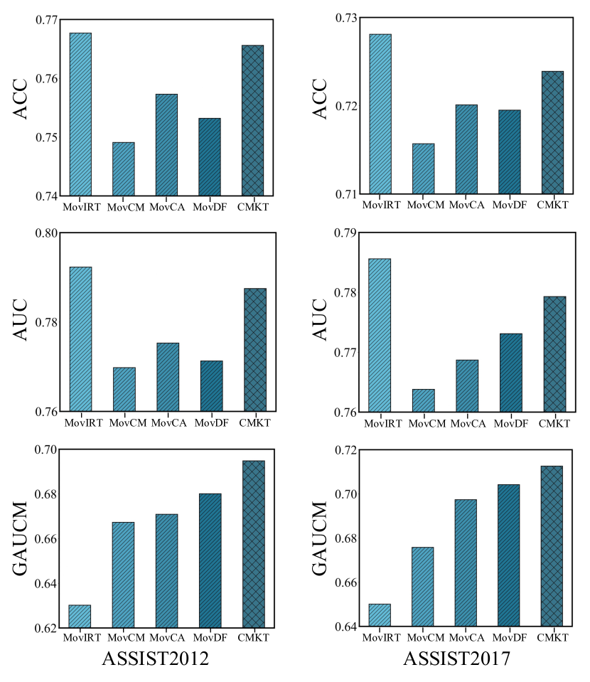
Figure 4. The experimental results of ablation study.

Table 3. The results of compatibility study, where * indicates p-value <0.05 in the significance test over the original model.

Model	ASSIST2009		ASSIST2012			ASSIST2017			EdNet		Algebra2005
	ACC	AUC	ACC	AUC	GAUCM	ACC	AUC	GAUCM	ACC	AUC	ACC	AUC
DKVMN	0.7302	0.7481	0.7359	0.7356	0.5432	0.6881	0.7195	0.5753	0.6806	0.7214	0.8015	0.8028
DKVMN + CM	0.7323*	0.7510*	0.7392*	0.7389*	0.5578*	0.6901*	0.7231*	0.5802*	0.6839*	0.7241*	0.8056*	0.8099*
GKT	0.7238	0.7436	0.7373	0.7293	0.5736	0.6994	0.7293	0.5872	0.6812	0.7240	0.8092	0.8125
GKT + CM	0.7249*	0.7448*	0.7399*	0.7357*	0.5792*	0.7013 *	0.7317*	0.5925*	0.6837*	0.7271*	0.8124*	0.8151*
SKT	0.7328	0.7516	0.7472	0.7421	0.5653	0.7133	0.7506	0.5814	0.6923	0.7343	0.8114	0.8161
SKT + CM	0.7335*	0.7529*	0.7491*	0.7450*	0.5728*	0.7167*	0.7542*	0.5896*	0.6941*	0.7355*	0.8142*	0.8189*
CKT	0.7353	0.7634	0.7395	0.7344	0.5751	0.7115	0.7412	0.5901	0.6823	0.7269	0.8113	0.8168
CKT + CM	0.7392*	0.7691*	0.7469*	0.7412*	0.5939*	0.7151*	0.7503*	0.6083*	0.6845*	0.7291*	0.8154*	0.8182*
LPKT	0.7401	0.7748	0.7592	0.7799	0.5862	0.7184	0.7759	0.6094	0.6912	0.7331	0.8123	0.8201
LPKT + CM	0.7421*	0.7762*	0.7623*	0.7841*	0.6343*	0.7201*	0.7773*	0.6416*	0.6928*	0.7351*	0.8134*	0.8229*

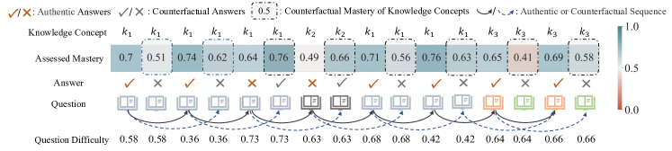
Figure 5. A case study of students’ mastery of knowledge concepts on the ASSIST2012 dataset. $k_{1}$ : Addition and Subtraction Positive Decimals. $k_{2}$: Ordering Positive Decimals. $k_{3}$: Multiplication and Division Positive Decimals.

5.6. Ablation Study (RQ2)

We conduct the ablation study with for comparative settings:
$\bullet$ MovCM removes the counterfactual restriction function.
$\bullet$ MovCA removes the virtual question constructed by concept difficulty (Eq. 7) and replace it with a randomly initialized vector.
$\bullet$ MovDF removes the regularization term of questions’ difficulty.
$\bullet$ MovIRT removes MIRT and replace it with a deep network.

Figure 4 shows the average results of five runs, indicating that all variants reduce CMKT’s performance in both datasets, with MovCM and MovIRT having the greatest impact on the GAUCM. The counterfactual constraint function (MovCM) can indicate the monotonicity of student learning progress, which is difficult to achieve with the prediction loss. By replacing MIRT with deep neural networks (MovIRT), the model’s predictive performance improves, but the interpretability of concept mastery evaluation suffers. Thus, it’s important to balance the predictive performance of the model with the reasonableness of the assess mastery value. Although removing MIRT improves the model’s prediction performance, it also decreases the GAUCM significantly. As such, we believe it’s worth sacrificing some predictability to obtain more reliable mastery results. MovCA causes more significant performance degradation of CMKT on ASSIST2012 than on ASSIST2017 due to the larger number of concepts in ASSIST2012. Eq. 7 connects the model’s input (i.e., representation of $p_{t}$) with the virtual question representation to expedite model convergence. Additionally, removing the difficulty regularization term of questions harms the model’s performance, but because ASSIST2017 has sufficient practice records per question, questions can still learn highly generalized representations, resulting in minor performance degradation.

5.7. Compatibility Study (RQ3)

Besides, we conduct compatibility study and present the results in Table 3, where +CM refers to the application of the counterfactual monotonicity constraints during the baseline models training. Table 3 shows that CM effectively improves GAUCM, as well as ACC and AUC metrics in the baselines, and LPKT shows greater performance improvement than other baselines. We believe that the reason is that the motivation of counterfactual monotonicity is similar to modeling the learning gain between two practices, and the CM loss complements LPKT’s design to achieve better performance. Additionally, we observe that all baselines still perform worse than CMKT after adding CM. We think this is because the prediction loss and structure of CMKT are specifically designed for monotonicity, enabling the CM to play a larger role. While the baselines use the deep network to predict responses, adding CM may lead to potential gradient conflicts. Therefore, it’s essential to design a reasonable structure for assessing students’ mastery of knowledge concepts, rather than merely introducing a specific training objective.

5.8. Visualization

To further comprehend students’ mastery of concepts, we randomly selected an 8-question, 3-concept student record from the ASSIST2012 dataset, as shown in Figure 5. We can find that the student’s mastery of $k_{1}$ is 0.7 when he correctly answer a question involving $k_{1}$ for the first time, which is higher than the mastery of counterfactual answers at 0.51. This phenomenon persists throughout the evolution process, verifying our model’s effectiveness in learning counterfactual monotonicity. Additionally, Figure 5 shows that a student’s mastery of the same concept varies when practicing different question involving that concept. This variation may be due to differences in question difficulty. If a student correctly answers more difficult questions, his learning gain should be greater than that of less difficult questions, resulting in a more significant improvement in concept mastery. That’s also why we should consider difficulty information in the knowledge extraction module.

6. Conclusions

In this paper, we propose a principled approach called Counterfactual Monotonic Knowledge Tracing (CMKT), which uses a type of counterfactual monotonicity to enhance the interpretability and semantic of assessed knowledge mastery values. Specifically, we first map students’ historical practice sequences to their concept mastery values. Then, by constructing counterfactual sample pairs and conducting pair-wise training, we can directly constrain the knowledge update process of students in the model at the concept level to ensure semantic information of the assessed knowledge mastery value. Meanwhile, to take full advantage of student response label information, we predict their responses by measuring the difference between their mastery value and the difficulty level of the question. A prediction loss of students’ responses is then used to facilitate model learning, together with the above counterfactual monotonic regularization term and a question difficulty regularization term. Finally, extensive experiments are conducted to verify the superiority of CMKT on five datasets based on a new metric called GAUCM and two commonly used ones.

- (1) Ashton Anderson, Daniel Huttenlocher, Jon Kleinberg, and Jure Leskovec. 2014. Engaging with massive online courses. In Proceedings of the 23rd international conference on World wide web (WWW). (Apr. 2014), 687–698.
- (2) Ghodai Abdelrahman, Qing Wang, and Bernardo Pereira Nunes. Knowledge Tracing: A Survey. 2023. ACM Computing Surveys. 55, 224 (2023), 1-37.
- (3) Bhaskar Bhattacharya and Desale Habtzghi. 2002. Median of the p value under the alternative hypothesis. The American Statistician 56, 3 (2002), 202–206.
- (4) Hugh Burns, Carol A Luckhardt, James W Parlett, and Carol L Redfield. 2014. Intelligent tutoring systems: Evolutions in design. Psychology Press.
- (5) Hao Cen, Kenneth Koedinger, and Brian Junker. 2006. Learning factors analysis – a general method for cognitive model evaluation and improvement. In International Conference on Intelligent Tutoring Systems. Springer, 164–175.
- (6) Song Cheng, Qi Liu, Enhong Chen, Zai Huang, Zhenya Huang, Yiying Chen, Haiping Ma, and Guoping Hu. DIRT: Deep Learning Enhanced Item Response Theory for Cognitive Diagnosis. In Proceedings of the 28th ACM International Conference on Information and Knowledge Management (CIKM). (Nov. 2019), 2397-2400.
- (7) Benoît Choffin, Fabrice Popineau, Yolaine Bourda and Jill-Jênn Vie. 2019. DAS3H: Modeling student learning and forgetting for Optimally scheduling distributed practice of skills. In Proceedings of the 12nd International Conference on Educational Data Mining (EDM). (Jul. 2019), 29-38.
- (8) Albert T Corbett and John R Anderson. 1994. Knowledge tracing: Modeling the acquisition of procedural knowledge. User Modeling and User-Adapted Interaction. 4, 4 (Dec. 1994), 253-278.
- (9) Mingzhi Chen, Quanlong Guan, Yizhou He, Zhenyu He, Liangda Fang, and Weiqi Luo. 2022. Knowledge Tracing Model with Learning and Forget- ting Behavior. In Proceedings of the 31st ACM International Conference on Information and Knowledge Management (CIKM). (Oct. 2022), 3863-3867.
- (10) Youngduck Choi, Youngnam Lee, Dongmin Shin, Junghyun Cho, Seoyon Park, Seewoo Lee, Jineon Baek, Chan Bae, Byungsoo Kim and Youngjun Jang. 2019. Ednet: A large-scale hierarchical dataset in education. In Proceedings of the 21th International Conference on Artificial Intelligence in Education (AIED). (2020), 69-73.
- (11) Mingyu Feng, Neil T. Heffernan and Kenneth R. Koedinger. 2009. Addressing the assessment challenge with an online system that tutors as it assesses. User Modeling and User-Adapted Interaction. 19, 3 (2009), 243-266.
- (12) Aritra Ghosh, Neil Heffernan and Andrew S. Lan. 2020. Context-Aware Attentive Knowledge Tracing. In Proceedings of the 26th ACM SIGKDD Conference on Knowledge Discovery and Data Mining (KDD). (Aug. 2020), 2330-2339.
- (13) Alan G Hawkes. 1971. Spectra of some self-exciting and mutually exciting point processes. Biometrika 58, 1 (1971), 83–90.
- (14) Edward H Haertel. 1989. Using Restricted Latent Class Models to Map The Skill Structure of Achievement Items. Journal of Educational Measurement 26, 4 (1989), 301–321.
- (15) Sepp Hochreiter and Jürgen Schmidhuber. 1997. Long short-term memory. Neural Computation 9, 8 (Nov. 1997), 1735–1780.
- (16) Diederik P. Kingma, Jimmy Ba. A method for stochastic optimization. In Proceedings of the 3rd International Conference on Learning Representations (ICLR Poster). 2014.
- (17) Andrew S. Lan and Richard G. Baraniuk. 2016. A Contextual Bandits Framework for Personalized Learning Action Selection. In Proceedings of the 9th International Conference on Educational Data Mining (ICDM). (Jul. 2016), 424–429.
- (18) Frederick Lord. 1980. Applications of Item Response Theory to Practical Testing Problems. Erlbaum Associates.
- (19) Qi Liu, Shuanghong Shen, Zhenya Huang and Enhong Chen. A Survey of Knowledge Tracing. arXiv preprint arXiv:2105.15106 (2021).
- (20) Ting Long, Yunfei Liu, Jian Shen, Weinan Zhang and Yong Yu. 2021. Tracing Knowledge State with Individual Cognition and Acquisition Estimation. In Proceedings of the 44th International ACM SIGIR Conference on Research and Development in Information Retrieval (SIGIR). (Jul. 2021), 173-182.
- (21) Yann LeCun, Léon Bottou, Yoshua Bengio, and Patrick Haffner. 1998. Gradient-based learning applied to document recognition. In Proceedings of the IEEE. 86, 11 (Nov. 1998), 2278–2324.
- (22) Sheng Li, Quanlong Guan, Liangda Fang, Fang Xiao, Zhenyu He, Yizhou He, and Weiqi Luo. 2022. Cognitive Diagnosis Focusing on Knowledge Concepts. In Proceedings of the 31st ACM International Conference on Information and Knowledge Management (CIKM). (Oct. 2022), 3272-3281.
- (23) Yunfei Liu, Yang Yang, Xianyu Chen, Jian Shen, Haifeng Zhang and Yong Yu. 2020. Improving Knowledge Tracing via Pre-training Question Embeddings. In Proceedings of the 29th International Joint Conference on Artificial Intelligence (IJCAI). (Jul. 2020), 1577-1583.
- (24) S-J. Mason, and N-E. Graham. Areas beneath the relative operating characteristics (ROC) and relative operating levels (ROL) curves: Statistical significance and interpretation. Quarterly Journal of the Royal Meteorological Society: A journal of the atmospheric sciences, applied meteorology and physical oceanography. 128(584): 2145–2166, 2002.
- (25) Haiping Ma, Manwei Li, Le Wu, Haifeng Zhang, Yunbo Cao, Xingyi Zhang, and Xuemin Zhao. 2022. Knowledge-Sensed Cognitive Diagnosis for Intel- ligent Education Platforms. In Proceedings of the 31st ACM International Conference on Information and Knowledge Management (CIKM). (Oct. 2022), 1451-1460.
- (26) Stephen L Morgan and Christopher Winship. 2015. Counterfactuals and causal inference. Cambridge University Press.
- (27) Hiromi Nakagawa, Yusuke Iwasawa and Yutaka Matsuo. 2019. Graph-based Knowledge Tracing: Modeling Student Proficiency Using Graph Neural Network. In IEEE/WIC/ACM International Conference on Web Intelligence (WI). (Oct. 2019), 156-163.
- (28) Amir Hossein Nabizadeh, Alípio Mário Jorge and José Paulo Leal. 2019. Estimating time and score uncertainty in generating successful learning paths under time constraints. Expert Systems-The Journal of Knowledge Engineering. (Feb. 2019).
- (29) Chris Piech, Jonathan Bassen, Jonathan Huang, Surya Ganguli, Mehran Sahami, Leonidas J Guibas and Jascha Sohl-Dickstein. 2015. Deep knowledge tracing. In Proceedings of Conference on Advances in Neural Information Processing Systems (NIPS). (Dec. 2015), 505–513.
- (30) Philip I. Pavlik, Hao Cen and Kenneth R. Koedinger. 2009. Performance Factors Analysis - A New Alternative to Knowledge Tracing. In Proceedings of the 14th International Conference on Artificial Intelligence in Education (AIED). (Jul. 2009), 531–538.
- (31) Shalini Pandey and George Karypis. 2019. A self attentive model for knowledge tracing. In Proceedings of the 12th International Conference on Educational Data Mining (EDM). (Jul. 2019), 384–389.
- (32) Zachary A. Pardos and Neil T. Heffernan. 2010. Modeling individualization in a Bayesian networks implementation of knowledge tracing. In Proceedings of the 18th International Conference on User Modeling, Adaptation and Personalization. (Jun. 2010), 255–266.
- (33) Judea Pearl. 2009. Causality. Cambridge University Press.
- (34) Mark D Reckase. 2009. Multidimensional item response theory models. In Multidimensional item response theory. 79–112.
- (35) Steffen Rendel. 2010. Factorization Machines. In Proceedings of 10th IEEE International Conference on Data Mining (EDM). (Dec. 2010), 995–1000.
- (36) Jason D. M. Rennie and Nathan Srebro. Loss Functions for Preference Levels: Regression with Discrete Ordered Labels. In Proceedings of the Nineteenth Inter- national Joint Conference on Artificial Intelligence (IJCAI). (Aug. 2005).
- (37) Paul R Rosenbaum. Testing the conditional independence and monotonicity assumptions of item response theory. Psychometrika. 1984, 49(3):425–435.
- (38) Adam Santoro, Sergey Bartunov, Matthew M. Botvinick, Daan Wierstra, Timothy P. Lillicrap. Meta-Learning with Memory-Augmented Neural Networks. In Proceedings of the 33nd International Conference on Machine Learning (ICLR). (Jun. 2016), 1842-1850.
- (39) Mohsen Sayyadiharikandeh, Jonathan Gordon, José Luis Ambite, and Kristina Lerman. 2019. Finding Prerequisite Relations using the Wikipedia Clickstream. In Companion Proceedings of the 2019 World Wide Web Conference (WWW Companion). (May. 2019), 1240-1247.
- (40) Xiangyu Song, Jianxin Li, Taotao Cai, Shuiqiao Yang, Tingting Yang, and Chengfei Liu. A survey on deep learning based knowledge tracing. Knowledge-Based Systems. 110036 (2022).
- (41) Shuanghong Shen, Zhenya Huang, Qi Liu, Yu Su, Shijin Wang, and Enhong Chen. 2022. Assessing Student’s Dynamic Knowledge State by Exploring the Question Difficulty Effect. In Proceedings of the 45th International ACM SIGIR Conference on Research and Development in Information Retrieval (SIGIR). (Jul. 2022), 427-437.
- (42) Shuanghong Shen, Qi Liu, Enhong Chen, Zhenya Huang, Wei Huang, Yu Yin, Yu Su and Shijin Wang. 2021. Learning Process-consistent Knowledge Tracing. In Proceedings of the 27th ACM SIGKDD Conference on Knowledge Discovery and Data Mining (KDD). (Aug. 2021), 1452-1460.
- (43) Shuanghong Shen, Qi Liu, Enhong Chen, Han Wu, Zhenya Huang, Weihao Zhao, Yu Su, Haiping Ma and Shijin Wang. 2020. Convolutional Knowledge Tracing: Modeling Individualization in Student Learning. In Proceedings of the 43rd International ACM SIGIR conference on research and development in Information Retrieval (SIGIR). (Jul. 2020), 1857–1860.
- (44) J. Stamper, A. Niculescu-Mizil, S. Ritter, G. Gordon and K. Koedinger. Algebra I 2005-2006 and Bridge to Algebra 2006-2007. Development data sets from KDD Cup 2010 Educational Data Mining Challenge. Find them at http://pslcdatashop.web.cmu.edu/KDDCup/downloads.jsp.
- (45) Shiwei Tong, Qi Liu, Wei Huang, Zhenya Huang, Enhong Chen, Chuanren Liu, Haiping Ma, and Shijin Wang. Structure-based Knowledge Tracing: An Influence Propagation View. In Proceedings of the 20th IEEE International Conference on Data Mining (ICDM). (Nov. 2020), 541–550.
- (46) Shiwei Tong, Qi Liu, Runlong Yu, Wei Huang, Zhenya Huang, Zachary A. Pardos, Weijie Jiang. Item Response Ranking for Cognitive Diagnosis. In Proceedings of the Thirtieth International Joint Conference on Artificial Intelligence (IJCAI). (Aug. 2021), 1750-1756.
- (47) Kurt VanLehn. 1988. Student modeling. Foundations of intelligent tutoring systems. 55 (1988), 78.
- (48) Ashish Vaswani, Noam Shazeer, Niki Parmar, Jakob Uszkoreit, Llion Jones, Aidan N Gomez, Łukasz Kaiser and Illia Polosukhin. 2017. Attention is All you Need. In Proceedings of 30th Conference on Advances in Neural Information Processing Systems (NIPS). (Dec. 2017), 5998–6008.
- (49) Jill-Jênn Vie and Hisashi Kashima. 2019. Knowledge Tracing Machines: Factorization Machines for Knowledge Tracing. In Proceedings of the 31th AAAI Conference on Artificial Intelligence (AAAI). 33, 01 (Jul. 2019), 750-757.
- (50) Fei Wang, Qi Liu, Enhong Chen, Zhenya Huang, Yuying Chen, Yu Yin, Zai Huang and Shijin Wang. 2020. Neural Cognitive Diagnosis for Intelligent Education Systems. In Proceedings of the 34th AAAI Conference on Artificial Intelligence (AAAI). (Feb.2020), 6153-6161.
- (51) Xin Wang, Wei Huang, Qi Liu, Yu Yin, Zhenya Huang, Le Wu, Jianhui Ma and Xue Wang. 2020. Fine-Grained Similarity Measurement between Educational Videos and Exercises. In Proceedings of the 28th ACM International Conference on Multimedia (MM). (Oct. 2020), 331–339.
- (52) Chenyang Wang, Weizhi Ma, Min Zhang, Chuancheng Lv, Fengyuan Wan, Huijie Lin, Taoran Tang, Yiqun Liu, Shaoping Ma. 2021. Temporal Cross- Effects in Knowledge Tracing. In Proceedings of the Fourteenth ACM Inter- national Conference on Web Search and Data Mining (WSDM). (Mar. 2021), 517-525.
- (53) Michael Yudelson, Kenneth R. Koedinger and Geoffrey J. Gordon. 2013. Individualized Bayesian knowledge tracing models. In Proceedings of 16th International Conference on Artificial Intelligence in Education (AIED). (Jul. 2013), 171–180.
- (54) Haiping Zhu, Feng Tian, Ke Wu, Nazaraf Shah, Yan Chen, Yifu Ni, Xinhui Zhang, Kuo-Ming Chao and Qinghua Zheng. 2018. A multi-constraint learning path recommendation algorithm based on knowledge map. Knowledge-Based Systems. (March. 2018), 102-114.
- (55) Han Zhu, Junqi Jin, Chang Tan, Fei Pan, Yifan Zeng, Han Li and Kun Gai. Optimized Cost per Click in Taobao Display Advertising. In 23th ACM international conference on Knowledge discovery and data mining (KDD). (Aug. 2017), 2191-2200.
- (56) Jiani Zhang, Xingjian Shi, Irwin King and Dit-Yan Yeung. 2017. Dynamic key-value memory networks for knowledge tracing. In Proceedings of the 26th International Conference on World Wide Web (WWW). (Apr. 2017), 765–774.
- (57) Juntao Zhang, Nanzhou Lin, Xuelong Zhang, Wei Song, Xiandi Yang, and Zhiyong Peng. 2022. Learning Concept Prerequisite Relations from Educational Data via Multi-Head Attention Variational Graph Auto-Encoders. In Proceedings of the 15th ACM International Conference on Web Search and Data Mining (WSDM). (Feb. 2022), 1377-1385.
- (58) Moyu Zhang, Xinning Zhu, Chunhong Zhang, Yang Ji, Feng Pan and Changchuan Yin. 2021. Multi-Factors Aware Dual-Attentional Knowledge Tracing. In Proceedings of the 30th ACM International Conference on Information and Knowledge Management (CIKM). (Oct. 2021), 2588-2597.
- (59) Tong Zhang. Solving large scale linear prediction problems using stochastic gradient descent algorithms. 2004. In Proceedings of the Twenty-first International Conference (ICML). (Jul. 2004).