POSIT: Promotion of Semantic Item Tail via Adversarial Learning

Abstract.

In many recommender problems, a handful of popular items (e.g. movies/TV shows, news etc.) can be dominant in recommendations for many users. However, we know that in a large catalog of items, users are likely interested in more than what is popular. The dominance of popular items may mean that users will not see items they would likely enjoy. In this paper, we propose a technique to overcome this problem using adversarial machine learning. We define a metric to translate user-level utility metric in terms of an advantage/disadvantage over items. We subsequently use that metric in an adversarial learning framework to systematically promote disadvantaged items. The resulting algorithm identifies semantically meaningful items that get promoted in the learning algorithm. In the empirical study, we evaluate the proposed technique on three publicly available datasets and four competitive baselines. The result shows that our proposed method not only improves the coverage, but also, surprisingly, improves the overall performance.

1. Introduction

Recommender systems are used extensively in many consumer web applications such as streaming services (Gomez-Uribe2015, ), video recommendations (youtube, ), news feed recommendations (10.1145/2835776.2835848, ; Agarwal2014, ) etc. The primary goal of recommender systems is to recommend appropriate items such that users are engaged, entertained or feel connected. The catalog of items can be movies, TV shows, news articles, videos, merchandise etc. Depending on how the training data is collected and how a model training is done many different types of biases can exist in a recommender system (10.1007/s10791-017-9312-z, ; chen2021bias, ; 10.1145/3109859.3109912, ); overcoming such biases is an important research direction in the field of recommender systems and many approaches have been proposed to go beyond accuracy and address some of these biases (e.g., (10.1145/2926720, ; 10.1145/1864708.1864761, )).

In this paper, we mainly focus on the so-called popularity bias (popularity-bias, ; popularity-bias-reranking, ) which is a particular type of bias where a recommender system recommends many popular items at a possible disadvantage to many other relevant items. The unpopular items, while have less user interaction, constitute the majority of the catalog and are typically referred to as the long tail of the catalog. Promoting such infrequent items from the long tail is potentially crucial to users’ satisfaction and a higher chance of success to every item. Different from the popular items, these infrequent items can coincide with the personalized taste, they can provide unexpected experience other than the mainstream popularity, motivate users to explore deeper into the catalog and evoke a sense of freshness (unexpected, ). On the supply side of items, many more items get a chance to succeed on the platform such that a handful of minority items do not suppress the chance of a vast majority of items.

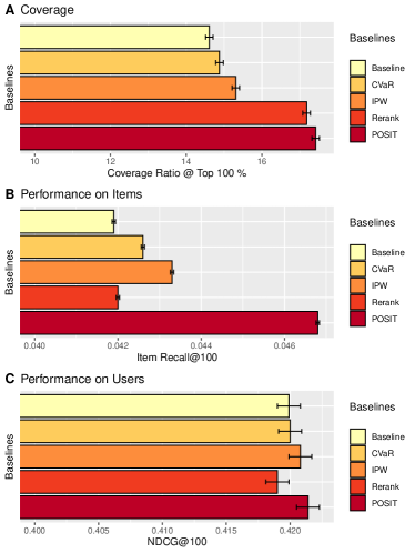
Figure 1. In figure (A), we compare the coverage ratio of unique recommended items divided by the upper-bound (see Equation 3). It reflects the coverage of unique and rare items, as well as inter-user diversity. In figure (B), we measure the performance of the recommendation on the item side (see Equation 9). In figure (C), we measure the performance on the user side. The experiments are conducting on the MovieLens 20 million dataset.

Figure 1(A) illustrates the concentration phenomenon of popular items on the MovieLens (movielens, ) dataset. We measure how many unique items are recommended at the top compared to the upper-limit of how many items can be recommended. A rigorous definition can be found in eq.(3). It shows that a strong baseline only covers about 15% items while our proposed technique can significantly improve coverage while not reducing the overall performance.

To alleviate this problem of a few items being concentrated at the top of the recommendation, an intuitive solution is to adjust the weight of items during learning. The weights are adjusted in a way that the more frequent items get down-weighted while the rare ones get up-weighted during training. While such a practice may alleviate the problem to some extent, there are many challenges associated with it. First, we need to clearly define an appropriate weight for each item while controlling how much we weigh one over the other. Second, it is unclear whether the frequency of the item alone should play such a big role in up-weighing an item or whether other factors should be considered.

Any technique that reduces the popularity bias and increases the coverage of items has the risk of reducing the overall performance of the recommender system. By promoting many more less frequent items, it is possible that the users would get even less utility compared to the more popular counterparts that could have been recommended. Figure 1(C) illustrates this trade-off. Observe that the performance of some baselines are quite affected with increasing coverage. In this paper, we propose a method to decrease the popularity bias, increase the coverage, while surprisingly, also improving the overall performance of recommender systems. Rather than directly optimizing over the tail of the catalog, our technique focuses on “semantically meaningful” tail via the use of an adversarial model. Figure 1(B) shows the large increase of performance on the tail by focusing on “semantically meaningful” tail.

The main contributions of our work are as follows. First, we identify that typically in a recommender system we care about user level ranking metrics, but for increasing item coverage we need to bridge the gap and make sense at an item level. We thus start with a user level metric and show how we can identify which items are at an advantage/disadvantage. Second, we use the defined metric in an adversarial model learning setting such that items at a disadvantage are promoted. Because of the smoothness of the adversarial model, much more semantically meaningful items are promoted rather than extreme outliers. Third, we show how the proposed objectives can be optimized. Finally, we show empirical results where we compare the proposed approach with several other baselines. The experiments show that while we significantly increase the coverage of items, we also improve the overall performance of recommendations. Finally, we show a number of empirical observations to shed light on how the proposed technique is able to achieve both accuracy and coverage.

The rest of the paper is organized as follows. We review other related work in Section 2. We define the problem setting and introduce the notations in 3. We define a metric to define the advantage of a item and further use it in an adversarial learning setting to optimize it in Section 4. We briefly introduce those compared baselines in Section 5. We show our empirical results on three publicly available datasets in Section 6. Finally, we conclude in Section 7.

2. Related Work

Adversarial machine learning has recently been gaining popularity (biggio2018wild, ; 2022_CVPR, ; DBLP:journals/corr/abs-1812-04948, ) in the literature. More recently, an instance level weight based adversary was proposed in (arl, ) the context of supervised learning and was further studied in the context of recommender systems (adv_friend, ). The work in (adv_friend, ) improves the model performance on users where baseline models had difficulty. Further, there have been other robust optimization approaches (10.1145/3485447.3512255, ) to improve the recommender system from a user performance perspective. However, to the best of our knowledge, our work constitutes a first attempt to study adversarial machine learning problem from an item side on recommender system.

Popularity bias is a popular topic in the recommender systems literature. There have been previous works on handling popularity bias (IPW, ; adomavicius2009toward, ; rockafellar2000optimization, ). Many of these approaches require identifying apriori which items are in the “long tail” and which ones are in the short-tail of recommendation. Their manual design process is difficult to address the popularity bias problem in a systematic manner. Compared to those approaches, we do not need to apriori identify which items are in the long tail versus short tail. We compare two competitive baselines in this category including IPW (IPW, ) and CVaR (rockafellar2000optimization, ) in Figure 3 and experiments. The results show our significant improvement in addressing the popularity bias problem.

Some of the proposed approaches  (adomavicius2009toward, ; 10.1145/3109859.3109912, ; popularity-bias-reranking, ; singh2018fairness, ; 10.1145/3471158.3472260, ) for handling popularity bias or ensuring some kind of fairness among items are based on post-processing rather than changing the learning algorithm itself. During post-processing, they re-rank the recommendations based on additional factors like frequency, exposure, merit etc. However, these methods involves a direct trade-off between performance and coverage while our method is focused on improving the underling model itself. Our method is able to alleviate popularity bias without sacrificing the performance. Moreover, the post-processing methods are complimentary to ours in the sense that they can be applied on top of any learned model. In our experiments, we include the Rerank (popularity-bias-reranking, ) baseline for comparison.

There is also work directly addressing producer-side fairness  (10.1145/3471158.3472260, ) in two sided market places. However, their framework requires additional information about the producers for item modeling. Differently, we leverage the user-side utility and convert that into an item side score and use it in an adversarial learning framework. This practice eliminates the need for extra producer information.

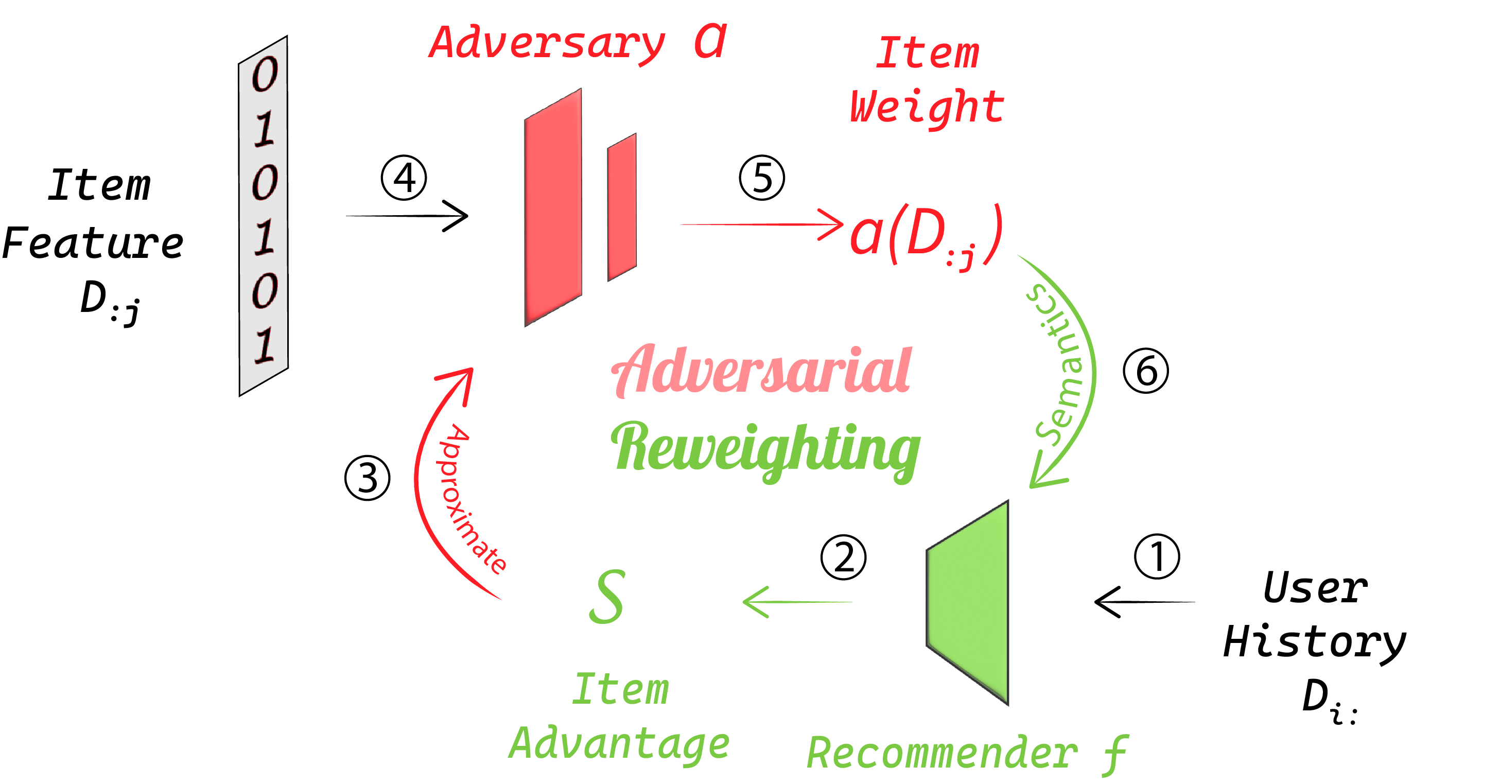
Figure 2. In this figure, we present the workflow of POSIT . Overall, it is an adversarial reweighting game consists of two parts. The green color indicates the recommendation learning part. And the red one indicates the adversarial learning part. In step \raisebox{-.9pt} {1}⃝, we first train the recommender system through user history. In step \raisebox{-.9pt} {2}⃝, we evaluate the advantage of each item based on the current recommendation results. In steps \raisebox{-.9pt} {3}⃝ and \raisebox{-.9pt} {4}⃝, we use the item advantage and item feature as the inputs to the adversary. In \raisebox{-.9pt} {5}⃝, we optimize the weights of each item generated from the adversary. Such optimized weight will emphasize those disadvantaged items. In \raisebox{-.9pt} {6}⃝, we use the optimized weights in training the recommender system. And repeat the previous procedures again until convergence.

3. Problem Setting and Preliminaries

In this paper, we focus on recommendation in an implicit-feedback setting. In this setting, we collect users’ interactions with a catalog of items. As a common assumption, the interaction of users indicates their preference. Unlike the explicit setting, the users will not directly express their preferences like a rating or score. The less strict assumption of implicit setting makes it important and popular as it closely aligns with many real world applications, where a majority of users do not give explicit feedback.

Consider a training dataset consisting of $|{\mathcal{I}}|$ items and $|{\mathcal{U}}|$ users, a user-item interaction matrix ${\bm{D}}\in\mathbf{R}^{|{\mathcal{U}}|\times|{\mathcal{I}}|}$. User $i$ has the interaction history ${\bm{D}}_{i}\in\{0,1\}^{|{\mathcal{I}}|}$, which means that the user $i$ has interacted with the items that are set to 1. When $D_{ij}=0$, it indicates the user $i$ didn’t interact with the item $j$. Such interactions can include a click, a buy or watching a movie. The goal is to learn a recommendation model $f:\{0,1\}^{|{\mathcal{I}}|}\rightarrow\mathbb{R}^{|{\mathcal{I}}|}$. The model gives a score to every item that can be used for item ranking. A higher score means it is more likely that a user would interact with it. Given a trained model, the goal then is to take a test user’s historically interacted items and rank the non-interacted items that are relevant to the user.

To evaluate the performance of recommendation system $f$ , we adopt a widely used ”Recall@k” as the metric. We also consider widely-used metrics like Normalized Discounted Cumulative Gain (NDCG) (Manning_etal_2008, ). Since these two metrics are heavily correlated with each other, we mainly focus on recall. Consider the preference over item $j$ for user $i$ as $D_{ij}$. The recommendation system scores each item via $f$ and ranks them by their scores for a particular user in the descendent order. Let the rank of item $j$ for user $i$ be $r_{ij}$. The Recall@K is defined as

(1) $$\mathrm{Recall@}k=\frac{1}{|{\mathcal{U}}|}\sum_{i\in{\mathcal{U}}}\frac{\sum_{j\in{\mathcal{I}}}\mathbbm{1}\left[D_{ij}=1\land r_{ij}\leq k\right]}{\min(k,\sum_{j\in{\mathcal{I}}}D_{ij})}\,.$$

Intuitively, it calculates the fraction of items within the top $k$ ranked items that are actually relevant for user $i$.

In addition to recall, we use coverage to measure how well the recommendation system can cover the entire catalog of items. Consider a batch of 100 randomly selected users ${\mathcal{U}}$. The coverage is defined as the unique numbers of items included in the top $k$ recommendations for these 100 users. Note that we fix the batch size 100 for fair comparisons. Choosing a larger batch size results in a similar observation, as shown in Section 6.1.

(2) $$\textrm{Coverage@}k=\left|\bigcup_{i\in{\mathcal{U}}}\left\{j\in{\mathcal{I}}|r_{ij}<k\right\}\right|$$

We report this number averaged among batches of 100 users. A higher coverage number indicates the system can cover diversified items for different users. We also report the ratio of converge against the possible upper-bound. The upper-bound is when each user is recommended with completely disjoint items. We defined the coverage ratio as follows:

(3) $$\textrm{Coverage Ratio@}k=\frac{\mathrm{Coverage@}k}{\min(k|{\mathcal{U}}|,|{\mathcal{I}}|)}$$

Loss. Before delving into the details, consider a recommendation system $f$ parameterized by ${\bm{W}}$, and a training loss for user $i$ and item $j$ as ${\mathcal{L}}(D_{i};{\bm{W}})_{j}$. The training objective can be described as

(4) $$\begin{split}\min_{{\bm{W}}}\sum_{ij}{\mathcal{L}}(D_{i};{\bm{W}})_{j}\end{split}$$

EASE. We consider a particular choice of loss function that was used in EASE (EASE, ) which is a strong baseline for recommender tasks. Different from common matrix factorization approaches, EASE leverages an item-similarity matrix ${\bm{W}}$ which captures the similarity between different items. However, to avoid learning the trivial solution of the identity matrix, EASE enforces the diagonal of the learned matrix to be $0$. The optimization can be written as

$$\min_{{\bm{W}}}\|D{\bm{W}}-D\|^{2}_{2}+\lambda\|{\bm{W}}\|^{2}_{2}$$

(5) $$s.t.,\text{diag}({\bm{W}})=0$$

We adopt EASE as the base recommender because its results on the implicit-feedback setting are very competitive. We will evaluate the performance of different methods applied on EASE. While mainly evaluating based on EASE, our method is general and can be applied to other base recommenders as well. Although at the time of training, a model like EASE (or Matrix Factorization) uses a squared loss, the loss is only a proxy at the time of optimization. The ultimate goal of the model trained is to still perform well on a ranking metric such as NDCG or Recall that we discussed above.

4. Adversarial Learning Approach

In this section, we first propose a way to identify items that are at a disadvantage and then propose a technique to promote such items. A workflow of our approach can be found in Figure (2).

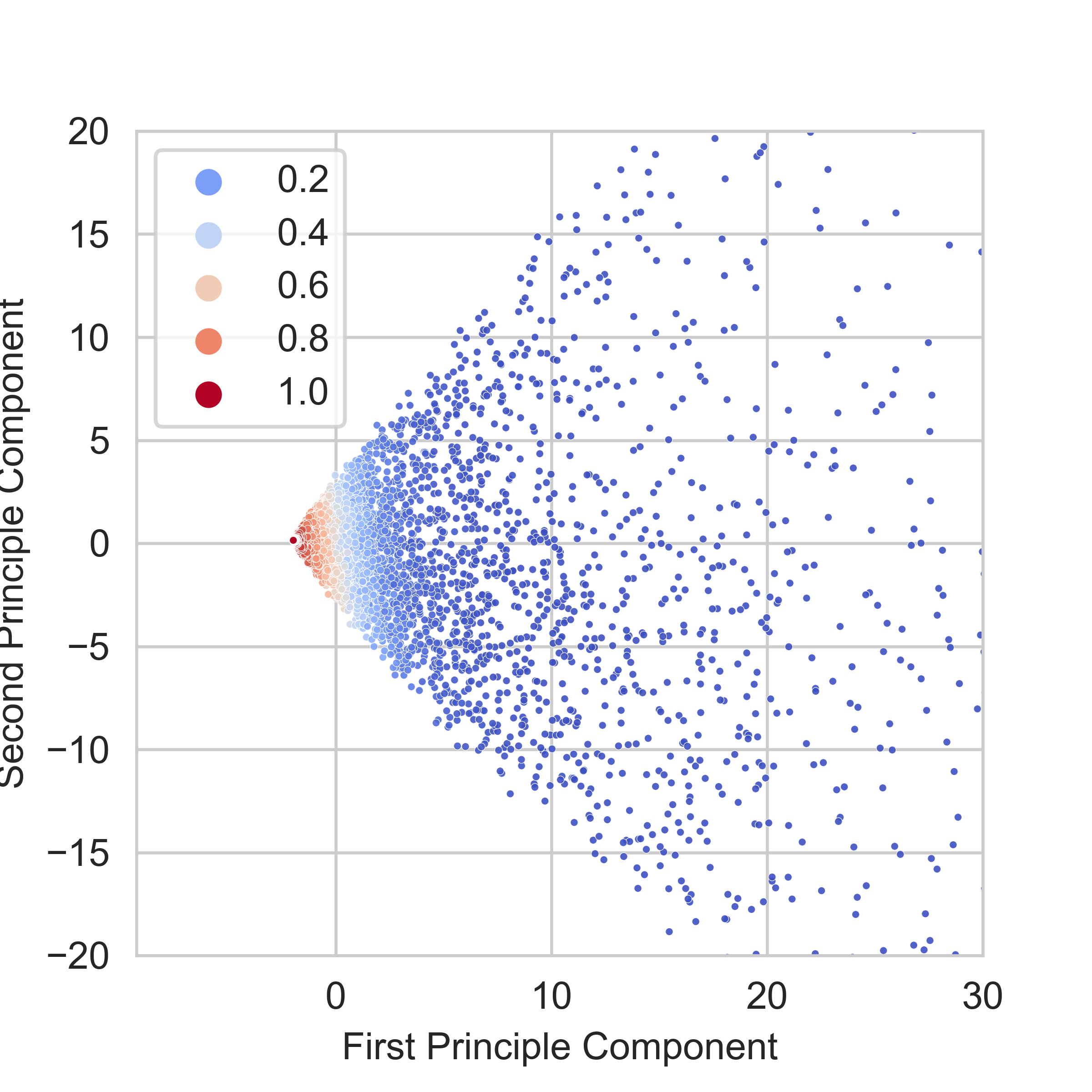
(a) Weight from POSIT

(b) Normalized Negative Advantage Score

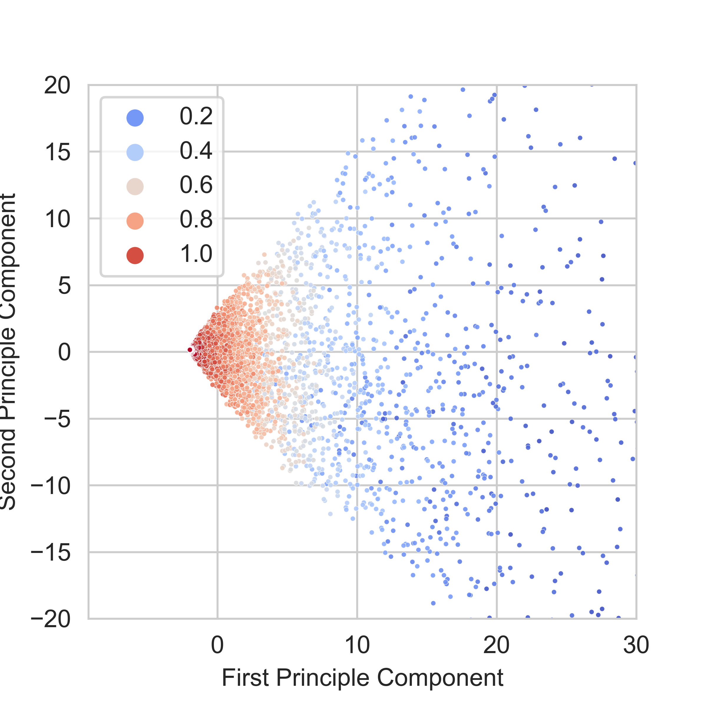
(c) Weight from the Best IPW model

Figure 3. Semantically Meaningful Weight. In this figure, we visualize the movies and their corresponding weights on the dataset MovieLens-20M obtained from different baselines. We visualize the movies by conducting Primary Component Analysis (PCA) on features of the movies. Each movie is represented as an point. The x-axis and y-axis are their first and second principle component. Close distance between points indicates the represented movies are similar. We color each point based on their assigned weight. A warm color represents a larger weight and a cold one indicates a smaller weight. Overall, we can observe that the points on the right part of each figure are scattered. The low density indicates outliers. In Figure (a), we show the weights from our method. Notice that our weights focus on semantically close points but much less on the outliers. Figure(b) shows the case where we directly use item advantage score to define the weight without an adversary. We can observe different colors are mixed everywhere. Compared with Figure (b), our adversary in Figure (a) effectively approximate an semantic tail from advantage score, and displays contrasting but progressive colors. In Figure (c), we demonstrate the weight obtained from best IPW model. Although it exhibits progressive colors, it doesn’t effectively capture the semantic tails as ours.

4.1. Identifying Items at a Disadvantage

As we discussed in the Introduction, a typical recommender system may bias towards certain types of items, like popular items. In this paper, we take an agnostic approach to such issues and adversarially remedy the problem by identifying items potentially at a disadvantage and promoting them. We will formally measure the disadvantage of an item by a score whose magnitude indicates the magnitude of the disadvantage. A proper choice of the advantage score is critical for the final results.

A major challenge to design an advantage score is the mismatch between training and evaluation metric. Usually, the training loss function, like $\ell_{2}$ loss (e.g. in eq. 5), is not directly used in evaluating a recommender system, although it may serve as a good proxy at training time. During evaluation, the performance of the recommender system is computed by ranking items at a user level. Thus, directly using training loss as the advantage score is not a good choice. Moreover, we empirically find that the disadvantaged items tend to have a small training loss compared to an average item due to the sparsity of the training data. This is however the opposite of what an advantage score should indicate. Due to sparse nature of the dataset, items with fewer interactions will tend to get smaller training losses . We therefore, focus on taking a user level ranking metric such as recall and attribute it to item level such that we can easily identify which items are at a disadvantage. This way, the item level metric will be directly related to the ultimate metric we care about in the system.

We use a metric derived from Recall@k as an example which we refer to as “Item Recall@k”. First, we generate a score matrix $R$ of the same size of $D$ by following the rules of Recall where $r_{ij}$ is the rank of item $j$ for user $i$:

(6) $$R_{ij}=\mathbbm{1}\left[D_{ij}=1\land r_{ij}\leq k\right]\,.$$

Next, we take the average of the score for each item. To decide the denominator for the average, we can either count the number of all users or the number of users with interactions to that item. The difference between these two options is whether the advantage score should consider the popularity bias or not. When using the size of whole users as the denominator, we essentially reflect the popularity bias in the advantage score. Since the denominator is the same for all items, the items that would end up in the top $k$ for more users would end up having a higher score. The other option removes the popularity bias normalizing by the number of interactions for that item. Therefore Item Recall@$k$ for item $j$ can be written as $S_{j}$ in two versions,

(7) $$S_{j}=\frac{1}{|{\mathcal{U}}|}\sum_{i\in{\mathcal{U}}}R_{ij}\quad$$ (Reflects popularity bias)

(8) $$S_{j}=\frac{1}{\sum_{i\in{\mathcal{U}}}D_{ij}}\sum_{i\in{\mathcal{U}}}R_{ij}\quad$$ (Without popularity bias)

When $S_{j}$ is high in equation (7), that means item $j$ is relevant and would end up in the top $k$ more often showing that the item being at an advantage given a ranking.

In Figure 7, we compare these two options and another metric frequency. The results shows that using item recall with popularity bias can empirically have a better performance. Thus, we will use eq.(7) which reflects popularity bias for optimization. During evaluation, since different items may have very different sizes of interactions, the metric with popularity bias cannot reflect the performance of the rare items. Thus we use eq.(8) for evaluation and define Item Recall@$k$ by aggregating over all items as the follows,

(9) $$\mathrm{Item\,Recall@}k=\frac{1}{|{\mathcal{I}}|}\sum_{j\in{\mathcal{I}}}\frac{\sum_{i\in{\mathcal{U}}}\mathbbm{1}\left[D_{ij}=1\land r_{ij}\leq k\right]}{\sum_{i\in{\mathcal{U}}}D_{ij}}\,.$$

Input : Interaction Matrix $D$, training epochs $T$, number of batches each epoch $L$, $\ell_{2}$-regularizer $\lambda$, top $k$ recommendation, Exponentially Moving Average(EMA) of advantage score $\hat{S}_{j}$ for each item $j$ using momentum $m$ and a SGD optimizer with learning rate $lr$

Output : A recommender $f$ and an adversary model $a$

1 Initialize $\hat{S}_{j}\leftarrow 0$, ${\bm{W}}\leftarrow 0$, parts of $\phi\leftarrow 0$

2 for $t\leftarrow 1$ to $T$ do

3       for $b\leftarrow 1$ to $L$ do

             $\hat{U}\subset{\mathcal{U}}$ // Sample a batch of users

             $\hat{S}_{j}\leftarrow(1-m)\hat{S}_{j}+mS_{j}$// Estimate $S_{j}$ from a batch

             $\bar{\alpha}_{j}=\frac{|{\mathcal{I}}|a(D_{:j};\psi)}{\sum_{j}a(D_{:j};\psi)}$ // Normalized weights

4             Optimize  $\min_{{\bm{W}}}\sum_{j\in{\mathcal{I}}}\bar{\alpha}_{j}\sum_{i\in\hat{U}}(D_{i:}{\bm{W}}-D_{i:})_{j}^{2}$ $+\lambda\|{\bm{W}}\|^{2}_{2}$

             $\textrm{diag}({\bm{W}})\leftarrow 0$ // Constraints of EASE

5             Optimize  $\max_{\psi}\sum_{j\in{\mathcal{I}}}\bar{a}_{j}(-\hat{S}_{j})$

6       end for

7      Evaluate on validation set and save the best model.

8       Update learning rate by a scheduler.

9 end for

Algorithm 1 The Procedure of POSIT

4.2. Adversarial Models

Once we have a score for each item $j$ defined above, we consider the following adversarially re-weighted learning formulation. Formally speaking, let us denotes the adversary model $a:\{0,1\}^{|{\mathcal{U}}|}\rightarrow\mathbb{R}$ parameterized by $\psi$, the feature of item $j$ as $D_{:j}$ and the item advantage score of item $j$ defined in eq.(7) as $S_{j}$, then we have the following formulation:

$$\textrm{Learner}: \min_{{\bm{W}}}\sum_{ij}a(D_{:j};\psi){\mathcal{L}}(D_{i};{\bm{W}})_{j}$$

(10) $$\textrm{Adversary}: \max_{\psi}\sum_{j\in{\mathcal{I}}}a(D_{:j};\psi)(-S_{j})\,.$$

The learner’s goal is to optimize the adversarially re-weighted loss. The adversary’s goal is to estimate a score for items at a disadvantage. In addition, the adversary model creates semantic weights based on the advantage scores, where semantic groups of disadvantaged items are implicitly identified and similar items will receive similar weights through the adversary model $a(D_{:j};\psi)$ parameterized by $\psi$. The semantic weight is important for alleviating the effects of outliers during re-weighting. Across different datasets in our evaluation, we find many outliers have a low item advantage score. By intuition, these outliers are at disadvantages and we need to increase the weight for those outliers in learning. However, increasing importance of such outliers during training without similarity between them will greatly reduce the performance of the recommender system. The reason is that the system is not able to generalize to those outliers without significantly impacting the majority. With a semantically meaningful adversarial score, we enforce smoothness and give similar scores to similar items. In figure 3, we visualize the phenomenon. The results show our adversary can indeed focus on the majority of disadvantaged items rather than a handful of outliers. We also typically regularize the adversarial model to limit its capacity.

It is worth noting that the advantage score $S_{j}$ is not a fixed value and are computed against the current model during the optimization. In formulation (10) we proposed a general form the learner and adversary that can be specialized to different recommender base models. In the following, we further rewrite the training paradigm under the baseline EASE by combining eq.(5) and eq.(10):

(11) $$\textrm{Learner}: \min_{{\bm{W}}}\sum_{i\in{\mathcal{U}},j\in{\mathcal{I}}}a(D_{:j};\psi)(D_{i:}{\bm{W}}-D_{i:})_{j}^{2}+\lambda\|{\bm{W}}\|^{2}_{2}$$

$$\text{s.t.,}\,\textrm{diag}({\bm{W}})=0$$

$$\textrm{Adversary}: \max_{\psi}\sum_{j\in{\mathcal{I}}}a(D_{:j};\psi)(-S_{j}),\quad$$

where $D_{i:}$ is the user $i$’s interaction history and ${\bm{W}}$ is the item similarity matrix learned by the EASE model. Note that in the summation and $S_{j}$ in eq.(11), we simultaneously optimize for each user and each item. This dependency on both dimensions makes it inappropriate for optimization in batches. To accommodate the batch optimization, we further maintain an Exponentially Moving Average (EMA) for values like advantage score $S_{j}$. These approximated values are updated gradually during iterations.

4.3. Implementation details

To limit the representation power and stabilize the training, we propose to build a small-capacity adversarial model and combine certain operators that tends to naturally filter out outliers.

Specifically, we combine normalization and bounded activation functions (e.g. Sigmoid) for filtering outliers. The idea of applying normalization before activations is to tune the value range of the inputs. Functions like Sigmoid will bound the output range and cap extremely large inputs, but less affect the values close to the average. Such large values usually indicates outliers. Denote the normalization operator as $n(x)=\tau\frac{x-\mu(x)}{\sigma(x)}$ where $\mu$ and $\sigma$ represents mean and standard deviation and $\tau$ an hyper-parameter, Hyperbolic Tangent function as $t(x)$, Sigmoid function as $s(x)$ and Fully Connected Layer as $H(x)$. Such operator combinations can be $t\circ n(x)$ or $s\circ n(x)$ depending on the desired output range. Note that we use an hyper-parameter $\tau$ to further control the degree of deviation of inputs. A larger $\tau$ filter more outliers. For the adversary, we choose $a(x)=t\circ n\circ H_{2}\circ s\circ n\circ H_{1}(x)$, we also compare different choices of structures in Figure 5.

In algorithm 1, we show the details of the algorithm. We sample a batch of users in line 4 and estimate the advantage score in Line 5. Line 6 normalizes the weights for stable optimization. In lines 7-9, we follow the optimization as described in eq.(11). We will update the learning rate and save the best model after each epoch.

Dataset	Number of			Interaction Ratio
	Users	Items	Interactions
Movie Lens	136k	20k	10M	3.6e-3
Netflix Prize	463k	17k	57M	7.2e-3
Million Song	571k	41k	34M	1.4e-3

Table 1. Characteristics of Datasets

Dataset	Method	Coverage@k
		Top 100	Top 50	Top 20
Movie Lens	POSIT	1793	1052	530
	IPW	1531	972	519
	CVar	1488	940	502
	Rerank	1718	948	490
	EASE	1461	922	489
	MP	100	50	20
Standard Deviation		$\pm 10$	$\pm 5$	$\pm 2$
Netflix Prize	POSIT	1968	1256	694
	IPW	1802	1179	670
	CVar	1795	1177	667
	Rerank	1950	1190	655
	EASE	1762	1153	654
	MP	100	50	20
Standard Deviation		$\pm 6$	$\pm 4$	$\pm 2$
Million Song	POSIT	6569	3692	1625
	IPW	6466	3673	1626
	CVar	6337	3556	1567
	Rerank	6368	3624	1609
	EASE	6304	3623	1609
	MP	100	50	20
Standard Deviation		$\pm 9$	$\pm 5$	$\pm 2$

Table 2. We report the coverage for five different methods in this Table. Here, $\pm$ represents the standard deviation of the coverage number of 100 users. For example, on Movie Lens, there are 10000 users in the test set. We fixed the order of user list for all the method. We split them as chunks of 100 users. We report the mean coverage and the standard deviation for each dataset excluding baseline MP. Best results within one standard deviation are highlighted.

Dataset	Method	Metric
		NDCG@K	Recall@K
		Top100	Top100	Top50	Top20
Movie Lens	POSIT	0.4214	0.6369	0.5244	0.3928
	IPW	0.4209	0.6364	0.5226	0.3926
	CVar	0.4200	0.6353	0.5210	0.3911
	Rerank	0.4190	0.6300	0.5199	0.3906
	EASE	0.4199	0.6356	0.5209	0.3906
	MP	0.1905	0.3300	0.2351	0.1617
Standard Deviation		$\pm 0.001$
Netflix Prize	POSIT	0.3953	0.5565	0.4472	0.3633
	IPW	0.3942	0.5560	0.4464	0.3625
	CVar	0.3933	0.5537	0.4449	0.3617
	Rerank	0.3919	0.5478	0.4435	0.3612
	EASE	0.3930	0.5541	0.4448	0.3613
	MP	0.1587	0.2743	0.1749	0.1161
Standard Deviation		$\pm 0.001$
Million Songs	POSIT	0.3915	0.5116	0.4290	0.3341
	IPW	0.3909	0.5099	0.4290	0.3340
	CVar	0.3839	0.5070	0.4240	0.3268
	Rerank	0.3896	0.5062	0.4278	0.3339
	EASE	0.3898	0.5084	0.4279	0.3339
	MP	0.0582	0.0986	0.0680	0.0427
Standard Deviation		$\pm 0.001$

Table 3. We report the performance comparison between five different methods here. In the table, $\pm$ represents the std. deviation of the 10 repeated runs on separate test sets.

5. Baselines

In this section, we introduce four other baselines IPW (IPW, ), CVar (rockafellar2000optimization, ), Rerank (adomavicius2009toward, ) and MP that we compare against in this paper.

IPW. Inverse Propensity Weighting (IPW) (IPW, ) assigns a weight inverse proportional to an item’s interaction probability. In this way, an infrequent item will receive a larger weight. To make this method more competitive, we further apply a power $\beta$ to the number and a normalization. We search and report the best $\beta$. Formally, the probability of interactions for item $j$ can be counted as $\frac{1}{|{\mathcal{U}}|}\sum_{i\in{\mathcal{I}}}D_{ij}$. The following weight $\bar{w}_{j}$ is applied for each item $j$ during training:

(12) $$w_{j}=\left(\frac{1}{|{\mathcal{U}}|}\sum_{i\in{\mathcal{I}}}D_{ij}\right)^{\beta},\quad\bar{w}_{j}=|{\mathcal{I}}|w_{j}\mathbin{/}(\sum_{j\in{\mathcal{I}}}w_{j})\,.$$

CVaR. Condition value at risk(CVaR) (rockafellar2000optimization, ) optimizes over only the tail of items. A tail contains the worst $\alpha$ percent performed items, which are measured by the training loss function. Furthermore, those out-of-tail items are replaced by an upper-bound value. Formally, consider the loss function $\sum_{i}{\mathcal{L}}(D_{i};{\bm{W}})_{j}$ as in eq.(4), a positive indicator $[x]_{+}=\max(0,x)$ and an additional variable $\beta_{1}$, we have the optimization goal

(13) $$\min_{{\bm{W}},\beta_{1}}\sum_{j\in{\mathcal{I}}}\left\{\beta_{1}+\frac{1}{\alpha}\left[\sum_{i\in gU}{\mathcal{L}}(D_{i};{\bm{W}})_{j}-\beta_{1}\right]_{+}\right\}\,.$$

An optimal solution will ensures that $\beta_{1}$ is the threshold of training loss that just separates the tail part and only the tail part of the loss is optimized.

Rerank. Rerank (adomavicius2009toward, ) promote items in the tail by post-processing during evaluation. Suppose a recommender ranks all the items into a list for some user based on the relevance $[i_{1},i_{2},...,i_{n}]$. Each item is associated with a relevance score $s$ such that $s_{1}\geq s_{2}...\geq s_{n}$. It partitions this recommendation results by two thresholds $T_{h}$ and $T_{l}$. The top recommendations are items with relevance $s_{j}\geq T_{h}$. The method will keep their order same as before. The tail recommendations are items with relevance $T_{h}\geq s_{j}\geq T_{l}$. They are re-sorted according to frequency of the item’s occurrence. Infrequent items will rank higher than before, but still rank lower than the top recommendations. Other recommendations with even less relevance are simply ignored as they represents irrelevant items. We fine-tune the two thresholds during evaluation and report the best result.

MP. The Most-Popularity (MP) algorithm ranks items solely based on their popularity, with more popular items receiving a higher rank. This baseline is included to provide an intuitive demonstration of the metrics on vanilla baselines.

Dataset	Method	Item Recall@k			Improve(%)
		100	50	20
Movie Lens	POSIT	0.0465	0.0294	0.0146	13.3%
	IPW	0.0433	0.0270	0.0131	4.4%
	CVaR	0.0426	0.0262	0.0127	2.0%
	Rerank	0.0419	0.0257	0.0123	0.0%
	EASE	0.0419	0.0257	0.0123	-
	MP	0.0067	0.0035	0.0016	-
Netflix Prize	POSIT	0.0958	0.0631	0.0342	23.9%
	IPW	0.0833	0.0526	0.0269	4.5%
	CVaR	0.0842	0.0532	0.0271	5.6%
	Rerank	0.0802	0.0502	0.0252	-0.1%
	EASE	0.0804	0.0502	0.0252	-
	MP	0.0083	0.0044	0.0019	-
Million Song	POSIT	0.248	0.203	0.143	1.2%
	IPW	0.246	0.202	0.142	0.4%
	CVaR	0.240	0.192	0.131	-0.4%
	Rerank	0.244	0.201	0.141	-0.2%
	EASE	0.245	0.201	0.141	-
	MP	0.003	0.002	0.001	-
Standard Deviation		$\pm 0.0004$

Table 4. In this table, we report the performance by Item Recall@k. This metric excludes the popularity bias and better reflects the effectiveness of different methods. We also report the average improvement of each method compared to the base recommender EASE.

6. Experiments

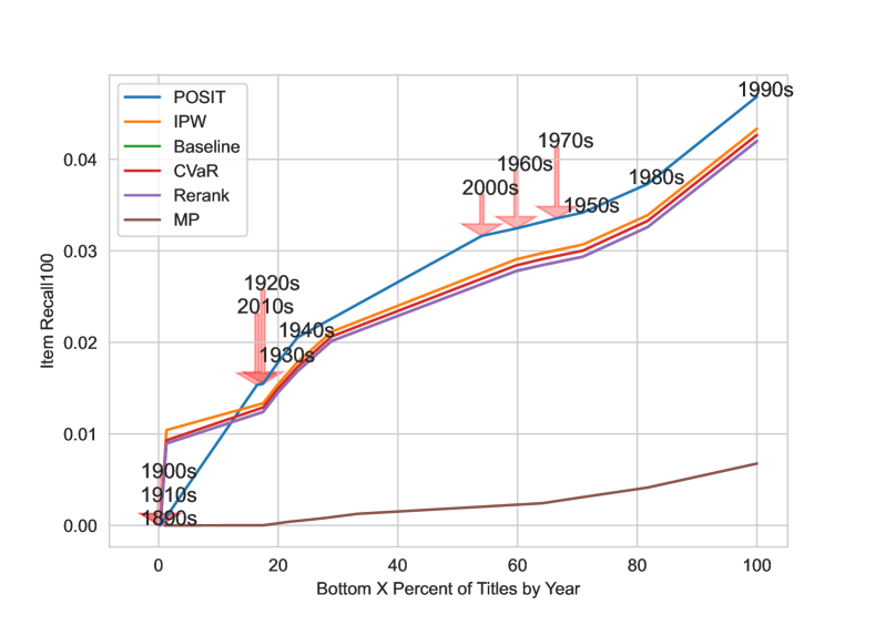
(a) Performance of Different Years

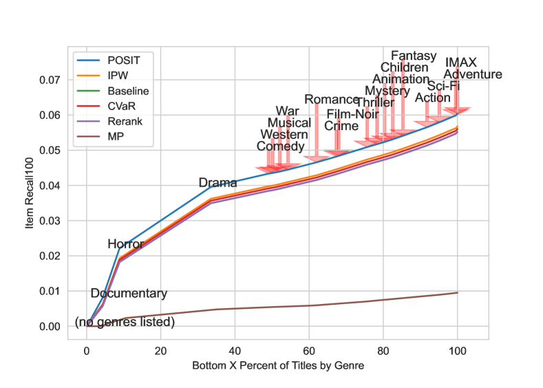
(b) Performance of Different Genres

Figure 4. In this figure, we report the Item Recall@100 for movies of different categories. We compare different methods on MovieLens. The performance is averaged for each category and sorted from the worst category to the best one. A low performance on specific categories, such as movies before 1910s and after 2010s, is due to limited data points in the dataset.

In this section, we report experiments on three large-scale datasets (summarized in Table 1), namely, MovieLens-20M (movielens, ), Netflix Prize (netflixprize, ) and the Million Song Dataset (millionsong, ) on the baselines introduced in Section 5. In the comparison, we conduct parameter sweeps for each baseline and report test metrics results for the best model on validation set. We follow the same procedures for all baselines except CVaR and Rerank. They have direct trade-offs between the performance and coverage. Reporting the model with the best performance will only fall back to the baseline EASE. Instead we report a representative model that has a comparative performance.

Specifically, we initialize the parameters ${\bm{W}}$ of EASE and the first layer of the adversary model as $0$. The reason is that those parameters directly take sparse inputs. Randomly initialized parameters will prevent a stable convergence as some of these values may hardly get chance to update themselves. We use SGD optimizer for our approach. For all baselines, we fine-tune the hyper-parameters including learning rate and $\ell_{2}$-regularizer $\lambda$. For POSIT , we also tune the learning rate of adversarial model and model structure (see Figure 5). For IPW, we tune the parameter $\beta$. We tune the parameter $\alpha$ for CVaR and $T_{h}$ and $T_{l}$ for Rerank.

Coverage. In Table 2 we report the coverage@k from different methods on the three datasets. We report coverage@k when $k=20,50,100$ for thorough evaluation. The calculation of coverage can be found in eq.(2). The result shows that our proposed method achieves competitive coverage number compared to other baselines consistently on three datasets. Specifically, our method improve nearly 20% on Coverage@100 compared to that of EASE on MovieLens dataset.While Rerank has a coverage that is close to POSIT when $k=100$, its trade-off towards coverage significantly impacts its performance. By comparing the results, we observe that the proposed method is much more effective under the scenarios when k is large or when the baseline has poor coverage. For example, the Coverage@100 of EASE on MovieLens is one fourth of that number on Million Song dataset. Correspondingly, the increase of coverage@100 on MovieLens is larger than that on Million Song. The benefits of promoting tails increase as the a natural baseline becomes more concentrated due to the training data.

Similarly, the improvement of Coverage@100 is larger than that of Coverage@20 on these three datasets. It is because the recommender seldom ranks the items from the tail to the very top places. Therefore, the benefits of promoting items from the tail will gradually add up to a larger $k$ value for some metric@k. And the metric with larger $k$ is quite important for users who explore deep into the catalog, such as frequent users or users with many interests.

Performance. Note that it is commonly assumed there is a trade-off between coverage and accuracy metric Recall@k. However, we surprisingly find POSIT achieves the best of the both worlds. Table 3 reports the performance metrics including Recall@K and NDCG@k. Note that our method achieves slightly better performance than all the other baselines on all three datasets. We observe a similar trend as in the case of coverage, where the improvement is larger given a large $k$. The improvement of POSIT is statistically significant (two standard deviation) on Netflix Prize, but not necessarily on the other two datasets. The reason is because popular items consists of the majority of interactions. Consequently, although our method has greatly improved the tail, the improvement is not necessarily reflected on the metric after averaging over the whole dataset. To overcome this issue, we further report the Item Recall@k (see eq.(9)) which focuses on the tail in Table 4. Unlike the Recall, this metric reflects the performance of the recommender on the tail. This is a more suitable metric as the all baselines aim at improving the tail. The result shows our method greatly outperforms the other baselines. Specifically, we improve the performance at most 23.9% compared to EASE, while the other methods don’t have a comparable result.

Semantic Group. In Figure 4, we report the performance over different categories of items on MovieLens. This dataset provides additional attributes associated with each movie including released years and genres. Since they constitute some kind of semantic information, we look at the performance over titles grouped by different years/genre. It is worth noting the semantic information like year and genre are not used by POSIT during learning. The result shows that semantically meaningful weights help improving the performance of different semantic groups without explicit labels while the baseline methods do not show any improvement for most of these groups.

Frequency Diversity. In table 5, we report the relative Gini Index of recommenders (gini_index, ; mcauley2022, ). It is the Gini Index on recommendations divided by the same index on training data. It represents the popularity-bias increase for a recommender system. A smaller value is better. A value greater than 1 indicates the learning algorithm increase the popularity bias. We can observe that our algorithm tends to have a smaller number compared to other baselines.

Method	Gini Ratio
	Movie Lens	Netflix Prize	Million Songs
POSIT	1.033	1.077	0.941
IPW	1.041	1.087	0.958
CVaR	1.042	1.089	0.995
Rerank	1.039	1.088	0.971
EASE	1.043	1.088	0.977
MP	1.089	1.146	1.662
Standard Deviation	$\pm 0.001$	$\pm 0.002$	$\pm 0.002$

Table 5. In this table, we show the Gini ratio between original dataset and the prediction from the model.

6.1. Ablation Study

In this section, we conduct ablation studies on various research questions(RQ) impacting the POSIT . We study one factor at a time, conduct parameter sweeps for other factors and report the best result. We will draw the Pareto frontier (pareto, ) between coverage and performance. A curve in the upper-right corner is better.

RQ1: How to design a good adversarial model for POSIT ?

We evaluated different adversarial model structures in Figure 5 and found that combining bounded activation and normalization leads to improved performance. This suggests that these operators effectively filter out outliers. Observe the large differences between the 2-layer models with or without such operators in Figure 5. Additionally our results also showed that the number of layers, or model capacity, is a crucial factor for the best performance. Specifically, a 2-layer MLP provides the best results. Furthermore, we found that a small model with only 10 hidden units performs well, as seen in Figure 6. The small size of the adversary, approximately $1\textrm{e-}3$ the size of the recommender, results in low computational overhead for POSIT .

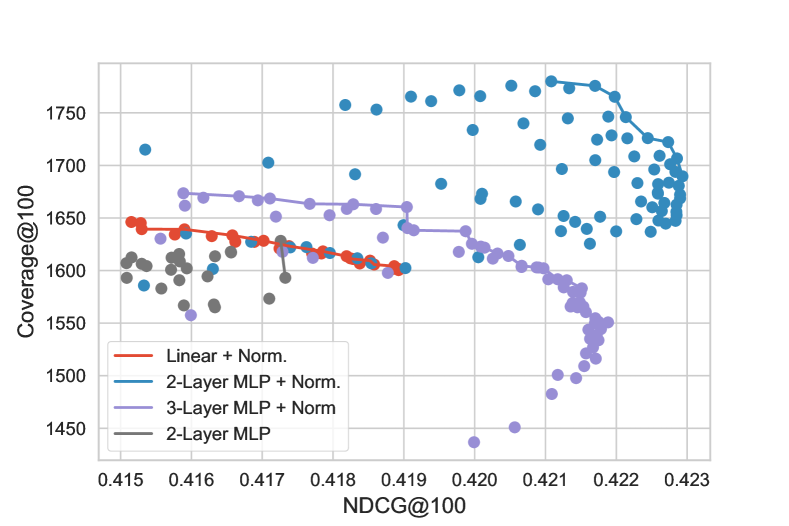
Figure 5. Comparison of Model Architecture. ”Norm” indicates an $\ell_{2}$ standardization applied before nonlinearity activation. ”MLP” indicates multi-layer perceptron. We use the tan-hyperbolic activation for intermediate layers and Sigmoid for the final output.

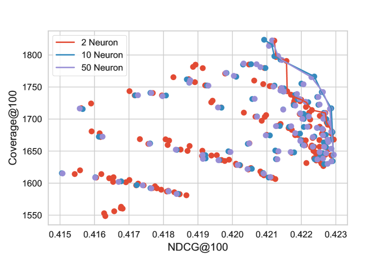
Figure 6. Comparison of Model Capacity. The label shows the number of hidden units on a 2-layer fully connected neural network for the adversary.

RQ2: Does the adversarial model require popularity bias to determine the weight?

We compare three candidates of advantage score using the same model in Figure 7. After conducting hyperparameter tuning, the results show that the advantage score without popularity bias performs similarly to the frequency score. Note that the frequency score is a key indicator of popularity bias. This supports that the score derived from user-level performance without popularity bias can effectively separate advantaged items and the disadvantaged ones. Furthermore, by combining popularity bias in eq.(7), we achieve better results than relying solely on popularity bias.

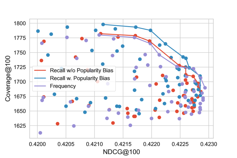
Figure 7. Comparison of Advantage Score

RQ3: How will batch size ($|{\mathcal{U}}|$) impact the results of Coverage@k in its definition (eq. 2)?
The batch size ($|{\mathcal{U}}|$ in (eq. 2)) used for calculating Coverage@k is fixed at 100 for fair comparisons. However, different batch sizes may emphasize different aspects of the coverage. When the batch size is small, such as 2, the metric focuses more on inter-user diversity. As the batch size increases larger, such as 100, the metric focuses on coverage of rare items. To gain a better understanding of POSIT ’s induction bias, we compare the Coverage@k under different user batch sizes, as shown in Table 6. The results shows that POSIT consistently produces competitive results across different batch sizes. This suggests that using batch size 100 strikes a good balance between dissimilarity and rare item coverage. Furthermore, we observe 60% improvement on POSIT compared with EASE when the batch size is 100. This highlights POSIT ’s ability to better promote rare items.

Method	User Batch Size in Coverage@100
	10	50	100	500	1000
POSIT	560	1309	1793	3386	4245
IPW	549	1190	1531	2431	2863
CVaR	543	1163	1488	2330	2734
Rerank	562	1284	1718	3108	3896
EASE	540	1147	1462	2260	2635
Standard Deviation	$\pm 2$	$\pm 5$	$\pm 10$	$\pm 18$	$\pm 40$

Table 6. In this table, we evaluate the Coverage@100 by varying user batch sizes on the MovieLens-20M dataset.

7. Conclusions

We proposed an adversarial learning approach called POSIT to reduce popularity bias through identifying semantic items forming tails. A key challenge was to take a user level metric and convert it to an item level score that could be exploited in an adversarial training. We analyzed how our method works through visualization studying many different aspects of the problem. POSIT was shown to achieve significantly better coverage and even an improvement in the overall performance on three large scale publicly available datasets.

Appendix A Experiment Details

We set training epochs $T=50$, $m=0.9$ in algorithm 1. We use a batch size of 1024 for MovieLens and 8192 for Million Song and Netflix Prize. We set the momentum of SGD optimizer as 0.9. We use 10k users for validation and another 10k users for testing on Movie Lens. We increase this number 10k to 40k on Netflix Prize and 50k on Million Song dataset respectively. Some datasets provide explicit preference information like Movie Lens. We follow the literature (EASE, ) and convert them into implicit settings through a preference threshold. Preference score greater than this threshold is set to 1 and otherwise it is set to 0.

We conduct the experiments on machines with 64G memory and 64 CPUs without GPU. This choice is due to budget concerns. We can finish the training on CPU as our model is relative small and reasonably fast enough on CPU. It typically takes 8 hours to train POSIT on MovieLens, 1.5 days on Netflix Prize and 1 day on Million Song. The major overhead is due to gradient optimization on these very large datasets. Speed can be potentially improved vastsly with GPU based training.

We conduct hyper-parameter search. Figure 8 is an example of the parameter search for baseline IPW on MovieLens. Note that we may fine-tune multiple factors and the results won’t necessarily be presented as a 2-dimensional figure. Table 7 lists all the hyper-parameters that is needed to exactly reproduce our results. We will also release our codes upon acceptance.

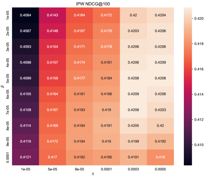
Figure 8. Example of Hyper-parameter Search for IPW on MovieLens

	Movie Lens	Netflix Prize	Million Song
Learning Rate(LR)	2.0	1.0	40.0
Adversarial LR	1.0	1.0	1.0
$\lambda$	8e-6	5e-5	1e-5
Advantage Score	As in Eq.(7)	As in Eq.(7)	As in Eq.(7)
$\tau$	1.5	1.0	0.5
Adversarial Model	2 Layer MLP	2 Layer MLP	2 Layer MLP

Table 7. Parameters used in our evaluation.

References

- [1] Himan Abdollahpouri, Robin Burke, and Bamshad Mobasher. Controlling popularity bias in learning-to-rank recommendation. In Proceedings of the Eleventh ACM Conference on Recommender Systems, RecSys ’17, page 42–46, New York, NY, USA, 2017. Association for Computing Machinery.
- [2] Panagiotis Adamopoulos and Alexander Tuzhilin. On unexpectedness in recommender systems: Or how to better expect the unexpected. ACM Trans. Intell. Syst. Technol., 5(4), dec 2014.
- [3] Gediminas Adomavicius and YoungOk Kwon. Toward more diverse recommendations: Item re-ranking methods for recommender systems. In Workshop on Information Technologies and Systems. Citeseer, 2009.
- [4] Deepak Agarwal, Bee-Chung Chen, Rupesh Gupta, Joshua Hartman, Qi He, Anand Iyer, Sumanth Kolar, Yiming Ma, Pannagadatta Shivaswamy, Ajit Singh, and Liang Zhang. Activity ranking in linkedin feed. In Proceedings of the 20th ACM SIGKDD International Conference on Knowledge Discovery and Data Mining, KDD ’14, pages 1603–1612, New York, NY, USA, 2014. ACM.
- [5] Lars Backstrom. Serving a billion personalized news feeds. In Proceedings of the Ninth ACM International Conference on Web Search and Data Mining, WSDM ’16, page 469, New York, NY, USA, 2016. Association for Computing Machinery.
- [6] Alejandro Bellogín, Pablo Castells, and Iván Cantador. Statistical biases in information retrieval metrics for recommender systems. Inf. Retr., 20(6):606–634, dec 2017.
- [7] James Bennett, Stan Lanning, et al. The netflix prize. In Proceedings of KDD cup and workshop, volume 2007, page 35. Citeseer, 2007.
- [8] Thierry Bertin-Mahieux, Daniel PW Ellis, Brian Whitman, and Paul Lamere. The million song dataset. 2011.
- [9] Battista Biggio and Fabio Roli. Wild patterns: Ten years after the rise of adversarial machine learning. Pattern Recognition, 84:317–331, 2018.
- [10] Jiawei Chen, Hande Dong, Xiang Wang, Fuli Feng, Meng Wang, and Xiangnan He. Bias and debias in recommender system: A survey and future directions, 2021.
- [11] Paul Covington, Jay Adams, and Emre Sargin. Deep neural networks for youtube recommendations. In Proceedings of the 10th ACM Conference on Recommender Systems, RecSys ’16, page 191–198, New York, NY, USA, 2016. Association for Computing Machinery.
- [12] Gerard Debreu. Valuation equilibrium and pareto optimum. Proceedings of the National Academy of Sciences of the United States of America, 40(7):588–592, 1954.
- [13] Frank A. Farris. The gini index and measures of inequality. The American Mathematical Monthly, 117(10):851–864, 2010.
- [14] Mouzhi Ge, Carla Delgado-Battenfeld, and Dietmar Jannach. Beyond accuracy: Evaluating recommender systems by coverage and serendipity. In Proceedings of the Fourth ACM Conference on Recommender Systems, RecSys ’10, page 257–260, New York, NY, USA, 2010. Association for Computing Machinery.
- [15] Carlos A. Gomez-Uribe and Neil Hunt. The netflix recommender system: Algorithms, business value, and innovation. ACM Trans. Manage. Inf. Syst., 6(4):13:1–13:19, December 2015.
- [16] F. Maxwell Harper and Joseph A. Konstan. The movielens datasets: History and context. ACM Trans. Interact. Intell. Syst., 5(4), dec 2015.
- [17] Bamshad Mobasher Himan Abdollahpouri, Robin Burke. Managing popularity bias in recommender systems with personalized re-ranking. In In Proceedings of The Thirty-Second International Flairs Conference, 2019.
- [18] Guido W. Imbens and Donald B. Rubin. Causal Inference for Statistics, Social, and Biomedical Sciences: An Introduction. Cambridge University Press, 2015.
- [19] Marius Kaminskas and Derek Bridge. Diversity, serendipity, novelty, and coverage: A survey and empirical analysis of beyond-accuracy objectives in recommender systems. ACM Trans. Interact. Intell. Syst., 7(1), dec 2016.
- [20] Tero Karras, Samuli Laine, and Timo Aila. A style-based generator architecture for generative adversarial networks. CoRR, abs/1812.04948, 2018.
- [21] Preethi Lahoti, Alex Beutel, Jilin Chen, Kang Lee, Flavien Prost, Nithum Thain, Xuezhi Wang, and Ed H. Chi. Fairness without demographics through adversarially reweighted learning. In Proceedings of the 34th International Conference on Neural Information Processing Systems, NIPS’20, Red Hook, NY, USA, 2020. Curran Associates Inc.
- [22] Christopher D. Manning, Prabhakar Raghavan, and Hinrich Schütze. An Introduction to Information Retrieval. Cambridge University Press, Cambridge, England, 2008.
- [23] Julian McAuley. Personalized Machine Learning. Cambridge University Press, in press.
- [24] R Tyrrell Rockafellar, Stanislav Uryasev, et al. Optimization of conditional value-at-risk. Journal of risk, 2:21–42, 2000.
- [25] Pannaga Shivaswamy and Dario Garcia-Garcia. Adversary or friend? an adversarial approach to improving recommender systems. In Proceedings of the 16th ACM Conference on Recommender Systems, RecSys ’22, page 369–377, New York, NY, USA, 2022. Association for Computing Machinery.
- [26] Ashudeep Singh and Thorsten Joachims. Fairness of exposure in rankings. In Proceedings of the 24th ACM SIGKDD International Conference on Knowledge Discovery & Data Mining, pages 2219–2228, 2018.
- [27] Harald Steck. Embarrassingly shallow autoencoders for sparse data. CoRR, abs/1905.03375, 2019.
- [28] Lequn Wang and Thorsten Joachims. User fairness, item fairness, and diversity for rankings in two-sided markets. In Proceedings of the 2021 ACM SIGIR International Conference on Theory of Information Retrieval, ICTIR ’21, page 23–41, New York, NY, USA, 2021. Association for Computing Machinery.
- [29] Hongyi Wen, Xinyang Yi, Tiansheng Yao, Jiaxi Tang, Lichan Hong, and Ed H. Chi. Distributionally-robust recommendations for improving worst-case user experience. In Proceedings of the ACM Web Conference 2022, WWW ’22, page 3606–3610, New York, NY, USA, 2022. Association for Computing Machinery.
- [30] Qiuling Xu, Guanhong Tao, and Xiangyu Zhang. Bounded adversarial attack on deep content features. In Proceedings of the IEEE/CVF Conference on Computer Vision and Pattern Recognition (CVPR), pages 15203–15212, June 2022.
- [31] Ziwei Zhu, Yun He, Xing Zhao, and James Caverlee. Popularity bias in dynamic recommendation. In Proceedings of the 27th ACM SIGKDD Conference on Knowledge Discovery ; Data Mining, KDD ’21, page 2439–2449, New York, NY, USA, 2021. Association for Computing Machinery.