Nonparametric Bayes multiresolution testing for high-dimensional rare events

Abstract

In a variety of application areas, there is interest in assessing evidence of differences in the intensity of event realizations between groups. For example, in cancer genomic studies collecting data on rare variants, the focus is on assessing whether and how the variant profile changes with the disease subtype. Motivated by this application, we develop multiresolution nonparametric Bayes tests for differential mutation rates across groups. The multiresolution approach yields fast and accurate detection of spatial clusters of rare variants, and our nonparametric Bayes framework provides great flexibility for modeling the intensities of rare variants. Some theoretical properties are also assessed, including weak consistency of our Dirichlet Process-Poisson-Gamma mixture over multiple resolutions. Simulation studies illustrate excellent small sample properties relative to competitors, and we apply the method to detect rare variants related to common variable immunodeficiency from whole exome sequencing data on 215 patients and over 60,027 control subjects.

1 Introduction

Rare variants, defined as ‘alternative forms of a gene that are present with a minor allele frequency (MAF) of less than 1%’, play a critical role in explaining the genetic contribution to complex diseases by accounting for disease risk and trait variability, previously unexplained by large genome-wide association studies focused on common variants (Pritchard,, 2001). In spite of the advent of low-cost parallel sequencing approaches and the resultant development of statistical and machine learning methods for rare variants (see Nicolae, (2016), Meng et al., (2020) and references therein), very few previous works fully characterize the spatial nature of the rare mutations while retaining robustness, power, and scalability to massive dimensions. In this paper, we develop a flexible, multi-scale method for assessing differences in rare mutation rates between groups by probabilistically modeling them as rare events across the whole genome.

Motivation The failure of single variant tests for whole-genome sequencing data has motivated a variety of rare variant association tests, ranging from burden tests (Morgenthaler and Thilly,, 2007; Li and Leal,, 2008) and adaptive burden tests (Lin and Tang,, 2011) to variance component tests, e.g. SKAT (sequence kernel association test) (Wu et al.,, 2011). Unfortunately, these approaches are computationally intractable for ultra-high dimensional problems, and they ignore the physical locations on the genome. An example of strong spatial clustering of mutations is shown in Fig. 1, taken from the tumor portal, on a known oncogene PIK3CA (Shayesteh et al.,, 1999). To address the localization of mutations within small genomic windows, Fier et al., (2012) used an adaptive weighting scheme, and Ionita-Laza et al., (2012) used scan-statistics (Kulldorff,, 1997) to find the maximum density region (MDR) for rare variants. Although scan-statistics incorporate spatial information, the fixed rate assumption is restrictive, and it allows for a single MDR, losing power in the absence of strong clustering and becoming computationally expensive. The computational complexity is $O(N\log N)$ for $N$ locations (assuming fixed cost for density evaluation of intervals), which is intractable for whole genome or whole exome data sets, worsened by the additional computational burden of permutation P-values.

Computational costs are a crucial consideration for analyzing these massive datasets. There are $35,192,888$ possible locations on a single chromosome 22 where a rare variant could be present, out of which 312,010 positions exhibit $\mbox{mean allelic frequency}\leq 5\%$ which is by far the smallest data set available on the 1000 Genomes Project. Even the whole-exome sequencing data, representing less than 2% of the genome, is too huge for a linear-time algorithm to handle. For example, the whole-exome sequencing data from Exome Aggregation Consortium that forms our control group in Section 5 has $6,053,186$ amino acid positions on $18,774$ different genes that could harbor a rare variant. There is a pressing need for scalable methods that incorporate spatial information, exploit sparsity to scale to huge dimensions (computationally and statistically), and appropriately characterize uncertainty in mutation rates.

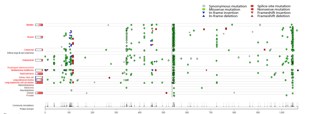
Figure 1: Spatial Clustering on PIK3CA

These considerations have led us to model the rare variants as realizations of a multiscale sparse point process that achieves a) computational speed by exploiting the sparsity, b) clustering of rare variants in smaller windows of a larger genomic region, and c) flexibility in modeling the unknown rate function. The sparsity and the clustering phenomenon of mutations imply that the intensity function will be effectively zero on a large majority of its domain and moderately higher in a few ‘hot spots’. We achieve computational efficiency by targeting the search to avoid genomic deserts containing no variants. We propose a binary tree-based, top-down multiresolution approach, in which we traverse from the coarsest resolution (whole genome) to finer resolutions, pruning irrelevant segments. The huge computational advantage stems from the fact that the number of expansion levels the tree must have to detect all clusters is on the order $O(\log N)$ (assuming fixed cost for density evaluation of intervals), which leads to a huge gain for very large $N$. Alternative multiresolution approaches have been used to detect high-density regions in applications including epidemiology (Neill et al.,, 2004), astronomy (van Dokkum et al.,, 2020), and medical imaging (Neill and Moore,, 2004), having better performance than scan statistics (Kulldorff,, 1997) or grid-based hierarchical clustering (Agrawal et al.,, 1998).

Building a flexible model for the intensity function is another key consideration as current parametric approaches for modeling sparse count data across different conditions, primarily based on zero-inflated Poisson (see Nie et al., (2006); Dhavala et al., (2010)) or zero-inflated negative binomial models (see Robinson et al., (2010); Hardcastle and Kelly, (2010); Anders and Huber, (2010)), do not offer sufficient flexibility in modeling the unknown mutation rate profile. The method proposed by Robinson et al., (2010), who model the variance as a function of both the mean and an additional component for incorporating the over-dispersion common to genomic data, is implemented in the popular R-package EdgeR. Other approaches involve Poisson-lognormal model (Sepúlveda et al.,, 2010; Rempala et al.,, 2011), truncated Poisson-Gamma model (Thygesen and Zwinderman,, 2006), and finite mixture of Poissons with a known number of components (Zuyderduyn,, 2007). Despite their popularity and success in genomic applications of relatively smaller scale, the Poisson model does not offer sufficient flexibility to model the number of variants in a given segment of the genome, in the sense that the Poisson mean also determines the rate and probability of zero variants. Instead, we propose a flexible nonparametric model that assumes that the variant frequencies are sampled from an infinite mixture of Poisson distributions that also allows for over-dispersion. Such mixture models naturally introduce latent parameters $\lambda_{i}$ that can be regarded as the true intensity at the $i^{th}$ location. Related non-parametric Poisson mixtures have been used in many different contexts (Trippa and Parmigiani,, 2011).

Our nonparametric Bayes modeling through a Dirichlet process prior on the Poisson rate parameters allows for great flexibility in modeling and performs well in estimating any true process $P_{0}$ in simulation studies (vide Section 4) and in practice identifies ‘differentially mutated’ regions from whole-exome sequencing data for $270$ patients with common-variable immunodeficiency symptom where the background mutation rate is obtained from a publicly available ExAC database on 60,276 individuals (vide Section 5). Theoretically, our DPM-Poisson-Gamma model leads to posterior consistency in estimating the marginal probability mass function of the rare variants, and intuitively, the consistency will continue to hold even after combining the estimates over multiple intervals (vide Section 3).

2 Modeling Framework

Our strategy is to partition the chromosome and prune ‘uninteresting’ intervals recursively. The key insight is that whole genome data admit a natural multiscale representation from the coarsest level (whole genome) to the finest level (individual variants). There is a rich literature on multiresolution methods that provide algorithms for multiscale decomposition of observed processes and have led to excellent tools for image denoising, classification, and data compression but have been under-explored in Genomics.

We employ a nonparametric approach of modeling the number of rare variants in each sub-interval of the genome induced by a space-partitioning balanced binary tree. The nonparametric model yields great flexibility and increasing power even in the case of weak clustering of variants. The multiresolution approach also allows for multiple clusters and speeds up the computation by a top-down pruning algorithm, as we describe below.

We can imagine the mutations as outcomes of a sparse point process across the genome, with the rate function potentially varying across groups. The baseline intensity rate is zero or extremely close to zero in an overwhelming majority of the locations on the genome (‘cold spots’) and substantially higher in biologically interesting segments of the genome (‘hot spots’). The differences between the groups manifest as shifts in the baseline rate functions that would be zero or very close to zero at the vast majority of the locations. Our goal is to calculate the posterior probability that the shift is everywhere zero (global null hypothesis) and the posterior probabilities for a sequence of increasingly local null hypotheses specific to genes or regions.

Formally, let $\mathit{T}$ be the entire region of interest, which in our case would be the whole genome or whole exome sequence under consideration. Let $\mathit{T}_{p}^{(l)}$, for all $p=1,\ldots,2^{l}$, for all $l=1,\ldots,L$ denote the partition of $\mathit{T}$ at resolution $l$, where $L$ denotes the total number of resolutions. Let $S_{p}^{(l)}=\{i:t_{i}\in\mathit{T}_{p}^{(l)}\}$ denote the indices of the events in the interval $\mathit{T}_{p}^{(l)}$, and let $n_{p}^{(l)}=|S_{p}^{(l)}|$ denote the cardinality of $S_{p}^{(l)}$. Let $\hat{\mathit{T}}_{p}^{(l)}$ denote $K$ equispaced points in the interval $\mathit{T}_{p}^{(l)}$, and let $y_{p,i}^{(l,1)}$ and $y_{p,i}^{(l,2)}$ denote the number of events for the two groups in the $i^{th}$ sub-interval induced by $\hat{\mathit{T}}_{p}^{(l)},\,i=1,\ldots,K+1$. Our goal is to test the differences in the underlying rates for the two sequences ${\bf y}_{p}^{(l,1)}$ and ${\bf y}_{p}^{(l,2)}$ for each $p$ and $l$.

We use the following semi-parametric model proposed by Guindani et al., (2014) for analyzing sequence count data on T-cell diversity for testing differential abundance (without the multi-resolution screening). Ignoring the resolution-specific subscripts $p$ and $l$ for the sake of notational clarity for the moment, let the true abundance rates for the two groups be $\lambda_{i}^{(1)}$ and $\lambda_{i}^{(2)}$. Then, the model for differential abundance is:

$$y_{i}^{(1)}\sim\mathrm{Poi}(\lambda_{i}^{(1)})\mbox{ and }y_{i}^{(2)}\sim\mathrm{Poi}(\lambda_{i}^{(2)})$$

$$[\lambda_{i}^{(1)}\mid P]\stackrel{{\scriptstyle iid}}{{\sim}}P$$

$$[\lambda_{i}^{(2)}\mid\lambda_{i}^{(1)},P]\stackrel{{\scriptstyle iid}}{{\sim}}\pi I(\lambda_{i}^{(1)}=\lambda_{i}^{(2)})+(1-\pi)P\;P\sim DP(M,P_{0}),$$ (1)

where $M=M^{(l)}$ is the precision parameter of the Dirichlet process $P=P^{(l)}$, and $P_{0}=P_{0,p}^{(l)}$ is the base measure, which is taken to be $P_{0,p}^{(l)}=\mathrm{Gam}(\alpha_{p}^{(l)},\beta_{p}^{(l)})$. Here $\alpha_{p}^{(l)},\beta_{p}^{(l)}$ respectively denote the resolution-specific shape and rate parameter of the Gamma distribution, which can be estimated from the data using an Empirical Bayes approach following the sequential approach of McAuliffe et al., (2006). The unique draws from the posterior in the inference phase are used to estimate the hyper-parameters of the Gamma base measure for the DP mixture model. A schematic diagram of the model is given in Figure 1. To facilitate posterior computation, we introduce a latent indicator variable $\mathbf{\gamma}$ such that

$$\gamma_{i}=\begin{cases}0&\mbox{if }\lambda_{i}^{(1)}=\lambda_{i}^{(2)}\\ 1&\mbox{ otherwise, }\end{cases}$$

where $\gamma_{i}\sim\mbox{Bern}(\pi)$. The posterior probability of differential abundance is given by:

$$\omega_{p,i}^{(l)}=P\left(\lambda_{p,i}^{(l,2)}\neq\lambda_{i}^{(l,1)}\mid y_{i}^{(1)},y_{i}^{(2)}\right).$$ (2)

To implement the Gibbs sampler, we can integrate out the base distribution $P_{0}$ and write the marginal likelihood of ${\bf y}$ as a negative binomial likelihood given the cluster configuration indices $s_{i,j}$ such that $s_{i,j}=k$ if $\lambda_{i,j}=\lambda_{j}^{*}$ as:

$$p({\bf y}\mid{\bf s})=\frac{1}{\prod_{i=1}^{K+1}y_{i,j}!}\frac{\beta^{\alpha J}}{\Gamma(\alpha)^{J}}\prod_{j=1}^{J}\frac{\Gamma(\alpha+\tilde{y_{j}})}{(\beta+N_{j})^{\alpha+\tilde{y_{j}}}},$$ (3)

where $\tilde{y_{j}}$ and $N_{j}$ denotes the sum of $y_{i,j}$’s belonging to $j^{th}$ cluster and its cardinality with $J$ being the total number of clusters. To update the cluster configurations $s_{i,j}$s, we first note that $s_{i,2}=s_{i,1}$ if $\gamma_{i}=0$, and $s_{i,j}$ follows a multinomial distribution with the probability vector given by:

$$P(s_{i,j}=k\mid\gamma_{i}=1,\mbox{rest})=\begin{cases}\frac{M}{M+\sum\gamma_{i}}p({\bf y}\mid{\bf s})\mbox{ for }k=J^{-i}+1\\ \frac{M}{M+\sum^{\sim k}\gamma_{i}}p({\bf y}\mid{\bf s})\mbox{ for }k\leq J^{-i},\end{cases}$$

where $`\mbox{rest}$’ denotes the remaining parameters $[\gamma_{-i},s_{-i,j},{\bf y}$], the symbol $\sum^{\sim k}$ denotes summation over all $s_{i,j}=k$. Furthermore, $p({\bf y}|{\bf s})$ is given by (3), with $\tilde{y_{j}}$ and $N_{j}$ replaced by $\tilde{y_{j}}^{-}$ and $N_{j}^{-}$, the sum of counts and size of the $j^{th}$ cluster with the $i^{th}$ observation deleted, and $J^{-i}$ denotes the maximum of $\{s_{-i,-j}\}$. On the other hand, the full conditional distribution for the differential abundance $\gamma_{i}$ can be derived as follows: $\gamma_{i}$ will be $1$ if $s_{i,2}\neq s_{i,1}$, and will follow a Bernoulli distribution with probability: $p(\gamma_{i}\mid s_{i,1}=s_{i,2},\mbox{rest})=p(s_{i,2}\mid\gamma_{i},s_{i,1}=s_{i,2},\mbox{rest})\times p(\gamma_{i})$.

We can carry out a multiple testing procedure for the $K+1$ paired observations in the $(p,l)^{th}$ sub-interval with a thresholding rule on $\omega_{p,i}^{(l)}$ as follows:

$$\mbox{Reject }H_{0,p}^{(i,l)}:\{\lambda_{p,i}^{(l,2)}=\lambda_{i}^{(l,1)}\}\mbox{ if }\omega_{p,i}^{(l)}>\xi,$$ (4)

for some suitable threshold $\xi$. For analyzing sequence count data on T-cell diversity, Guindani et al., (2014) proposed a related nonparametric method for testing differential abundance (without the multi-resolution screening), that was shown to be more powerful than existing parametric procedures.

This gives us a way of pruning intervals that cannot possibly contain any differentially mutated sub-regions since the shift in the mutation rate across the groups would be essentially zero at the vast majority of the locations. We do this by calculating the probability of a ‘global null’ hypothesis $H_{0,p}^{(l)}$ restricted to each partition $\mathit{T}_{p}^{(l)}$, $p=1,\ldots,2^{l}$ and pruning the interval if it exceeds a predetermined threshold.

In particular, we test the following ‘global’ hypothesis within each partition:

• $H_{0,p}^{(l)}$: there is no difference in mutation rates in the two groups on the partition $\mathit{T}_{p}^{(l)}$.

• $H_{A,p}^{(l)}$: at least one of the $K+1$ sub-interval of $\mathit{T}_{p}^{(l)}$ has a difference in the mutation rates across the groups.

The posterior probabilities for the global null can be obtained as a function of the marginal likelihoods obtained from the hierarchical model above, e.g., the posterior probability of global association is the sum of the posterior probabilities of all non-null models. For the present case, we assume independence across different sub-regions and simply reject the global null if $\prod_{i=1}^{K+1}(1-\omega_{p,i}^{(l)})<(1-\xi)^{K+1}$. The steps of the method are outlined in Algorithm 1.

Figure 2: Bayesian Nonparametric Model for Testing Differences

Algorithm 1: Multiscale NP-BayesTest

1:  Input: Count vectors ${\bf y}_{1},{\bf y}_{2}$, positions $J$, domain-set $\mathit{T}$, depth of the binary tree $L$, threshold $\xi$.

2:  for $l$ = 1 to $L$ do

3:     Sort all domains $T\in\mathit{T}^{l}$ by positions $J$.

4:     for all intervals $T\in\mathit{T}^{l}$ do

5:        Let ${\bf y}_{j}^{T};j=1,2$ and $J^{T}$ be the counts and the position-vector restricted to $T$.

6:        Calculate $\omega_{i}^{T}=P(\lambda_{i,1}\neq\lambda_{i,2}|{\bf y}_{1},{\bf y}_{2}),\;i=1,\ldots,|J^{T}|$.

7:        Calculate probability of global association $P_{H_{0}}(T)=\prod(1-\omega_{i}^{T})$.

8:        if $p_{H_{0}}^{T}>\xi^{|{\bf J}^{T}|}(\mbox{global threshold})$ then

9:           Prune interval $T$.

10:           Update $\mathit{T}\Leftarrow\mathit{T}\setminus T$, $J\Leftarrow J\setminus\{J\in T\}$.

11:        end if

12:     end for

13:  end for

A crucial issue is the choice of partitions and the depth of resolution. In the absence of any prior information about the location of the hot and cold spots, one would partition the genome using a balanced binary tree with partitioning informed by the posterior probabilities.

3 Theoretical Properties: Weak Consistency

We show that our proposed Dirichlet process mixture leads to posterior consistency in estimating the marginal probability mass function $P_{0}$ of the rare variants, and the consistency will continue to hold even after combining the estimates over multiple intervals. It will be interesting to settle theoretically if a multiresolution DPM model will put most of its posterior mass on a class of sparse density functions for the rate parameters. Although a thorough investigation of the properties of the induced multiple testing procedure for comparing the true abundances across groups is beyond the scope of the current article, we conjecture that the multiple testing rule in (4) will enjoy asymptotic optimality properties similar to Bogdan et al., (2011).

3.1 Dirichlet mixture of Poisson

Let $p_{\lambda}$ denote the Poisson probability mass function with mean $\lambda$. Let $\bm{\Theta}=\mathbb{R}^{+}$, and $\mathcal{M}$ be the set of probability measures on $\mathbb{R}^{+}$. For $P\in\mathcal{M}$, $f_{P}$ denotes the density:

$$f_{P}(i)=\int_{0}^{\infty}p_{\lambda}(i)dP(\lambda),i\in\mathbb{N}$$

Let $\mathcal{F}_{\mathbb{N}}$ be the set of all probability mass functions in $\mathbb{N}$. Then the prior $\Pi$ on $\mathcal{M}$ induces a prior on $\mathcal{F}_{\mathbb{N}}$ through the map $f_{P}=\int p_{\lambda}dP(\lambda)$, which we continue to denote by $\Pi$. Our model can be written as $P\sim\Pi$ and given $P$, $X_{1},\ldots,X_{n}\sim f_{P}$. Theorem 1 gives conditions for a class of densities to be in the K-L support of $\Pi$ and hence weakly consistent. The proof is similar to Theorem 3 in Ghosal et al., (1999) where they prove weak consistency for location mixtures of Gaussians for density estimation.

Theorem 1.

Let the true density $f_{0}\equiv f_{P_{0}}$ be of the form $f_{P_{0}}(j)=\int p_{\lambda}(j)dP_{0}(\lambda)$ for $j=1,2,\ldots$ and let $K_{\epsilon}(f_{0})$ be the $\epsilon$-weak neighborhood of $f_{0}$. If $P_{0}$ is compactly supported and belongs to the support of $\Pi$ , then $\Pi(K_{\epsilon}(f_{0}))>0$ for all $\epsilon>0$.

This proves the weak consistency for the case where the true mass function is a Poisson or a mixture of Poissons over a compact set. We present the proof below.

Proof.

Suppose $P_{0}[l,u]=1$ for some $u>l>0$. This implies, $\Pi\{P:P[l,u]>\frac{1}{2}\}>0,$ since $P_{0}$ is in the weak support of $\Pi$. For $\eta>0$, choose $k$ such that $\sum_{j>k}\mathrm{max}(1,j)f_{0}(j)<\eta$. We write:

$$\sum_{j=0}^{\infty}f_{P_{0}}(j)\log\left(\frac{f_{P_{0}}(j)}{f_{P}(j)}\right)=\sum_{j\leq k}f_{0}\log\frac{f_{P_{0}}}{f_{P}}+\sum_{j>k}f_{0}\log\frac{f_{P_{0}}}{f_{P}}.$$

Consider the second term:

$$\sum_{j>k}f_{0}\log\frac{f_{P_{0}}}{f_{P}} \leq\sum_{j>k}f_{0}(j)\log\left(\frac{\int_{l}^{u}p_{\lambda}(j)dP_{0}(\lambda)}{\int_{l}^{u}p_{\lambda}(j)dP(\lambda)}\right)$$

$$\leq\sum_{j>k}f_{0}(j)\log\left(\frac{\int_{l}^{u}\lambda^{j}e^{-\lambda}dP_{0}(\lambda)}{\int_{l}^{u}\lambda^{j}e^{-\lambda}dP(\lambda)}\right)\leq\sum_{j>k}f_{0}(j)\log\left(\frac{u^{j}e^{-l}}{l^{j}e^{-u}\frac{1}{2}}\right)$$

$$=\sum_{j>k}f_{0}(j)\{j\log(u/l)+(u-l)+\log 2\}\leq\eta\{\log(u/l)+(u-l)+\log 2\}.$$

Now consider the first term $\sum_{j\leq k}f_{0}\log\frac{f_{P_{0}}}{f_{P}}.$ Note that $\inf_{0\leq j\leq k}\inf_{l\leq\lambda\leq u}p_{\lambda}(j)=c>0$. Let

$$E =\left\{P:\left|\int p_{\lambda}(j)dP(\lambda)-\int p_{\lambda}(j)dP_{0}(\lambda)\right|<c\delta,\;j\leq k\right\}.$$

Since $E$ is a weak neighbourhood of $P_{0}$, $\Pi(E)>0$. Take $P\in E$. For such a P,

$$\left|\int p_{\lambda}(j)dP(\lambda)-\int p_{\lambda}(j)dP_{0}(\lambda)\right|<c\delta,$$

and hence,

$$\left|\frac{\int p_{\lambda}(j)dP(\lambda)}{\int p_{\lambda}(j)dP_{0}(\lambda)}-1\right|<\delta\Rightarrow\left|\frac{\int p_{\lambda}(j)dP_{0}(\lambda)}{\int p_{\lambda}(j)dP(\lambda)}-1\right|<\frac{\delta}{1-\delta}.$$

Thus, we have proved that for $P$ in a set of positive $\Pi$-probability,

$$\sum_{j=0}^{\infty}f_{P_{0}}(j)\log\left(\frac{f_{P}(0)(j)}{f_{P}(j)}\right) \leq\frac{\delta}{1-\delta}+\eta\{\log(u/l)+(u-l)+\log 2\}.$$

One can choose $\eta$ and $\delta$ so that for any $u>l>0$ the RHS is less than $\epsilon$. This completes the proof. ∎

Consistency over multiple resolutions Consider the balanced binary tree in Algorithm 1, where at level $l$ we partition the interval $\mathit{T}$ in $2^{l}$ intervals, denoted by $\mathit{T}_{p}^{(l)}$. We model the counts $y_{p}^{(l)}$ belonging to the interval ${\mathit{T}}_{p}^{(l)}$ as a Dirichlet Mixture of Poisson which possess weak consistency, and now we show that the weak consistency holds even when we combine estimates of probability mass functions (PMF) across partition to obtain an estimate of the true PMF for the entire interval $T$, for any resolution $l$. To see this, denote the aggregated PMFs as $f_{0}^{(l)}=\sum_{p}f_{0,p}^{(l)}$ and $f^{(l)}=\sum_{p}f_{p}^{(l)}$. By the weak consistency of DPM-Poisson, for any $\epsilon>0$,

$$\sum_{j}f_{0,p}^{(l)}(j)\log\frac{f_{0,p}^{(l)}(j)}{f_{p}^{(l)}(j)}<\epsilon,\;\mathrm{for\,all}\;l=1,\ldots,L\mbox{ and }p=1,\ldots,2^{l}.$$

We want to show that the weak consistency holds even when we aggregate over the partitions, that is, for all $l=1,\ldots,L,$ and for all $\epsilon>0$,

$$\sum_{j}f_{0}^{(l)}(j)\log\frac{f_{0}^{(l)}(j)}{f^{(l)}(j)} =\sum_{j}\sum_{p=1}^{2^{l}}f_{0,p}^{(l)}(j)\log\frac{\sum_{p=1}^{2^{l}}f_{0,p}^{(l)}(j)}{\sum_{p=1}^{2^{l}}f_{p}^{(l)}(j)}<\epsilon.$$

We first state the following lemma: a well known result about convexity of K-L divergence:

Lemma 2.

The K-L distance $D(f||g)$ is convex in the pair $(f,g)$, i.e. if $(f_{1},g_{1})$ and $(f_{2},g_{2})$ are two pairs of PMFs,

$$D \left(\alpha f_{1}+(1-\alpha)f_{2}||\alpha g_{1}+(1-\alpha)g_{2}\right)\leq\alpha D\left(f_{1}||g_{1}\right)+(1-\alpha)D\left(f_{2}||g_{2}\right).$$

This property can be generalized to $P$ pairs $(f_{p},g_{p}),\,p=1,\ldots,P$ and weights $\omega_{p}\geq 0,p=1,\ldots,P$, $\sum\omega_{p}=1$, i.e.,

$$D\left(\sum\omega_{p}f_{p}||\sum\omega_{p}g_{p}\right)\leq\sum\omega_{p}D(f_{p}||g_{p})$$

Taking $f_{p}=f_{0,p}^{(l)},g_{p}=f_{p}^{(l)}$ and $\omega_{p}=2^{-l}$ for $p=1,\ldots,2^{l}$, it follows from the above lemma that:

$$D(\sum_{p=1}^{2^{l}}f_{0,p}^{(l)}||\sum_{p=1}^{2^{l}}f_{p}^{(l)})\leq\sum_{p=1}^{2^{l}}D(f_{0,p}^{(l)}||f_{p}^{(l)})$$

The result follows by noting that with positive $\Pi$-probability, $D(f_{0,p}^{(l)}||f_{p}^{(l)})<\epsilon/2^{l}$ for all $p=1,\ldots,2^{l}$.

4 Numerical Experiments

To illustrate the performance of the induced decision rule (4), we consider the problem of testing for differences between realizations of two inhomogeneous Poisson processes having intensity functions:

$$\lambda_{1}(x) =2\exp\left(-\{(x-50)/10\}^{2}\right)+20\exp\left(-\{(x-10)/10\}^{2}\right);x\in\mathbb{R}^{+}$$

$$\lambda_{2}(x) =20\exp\left(-\{(x-50)/10\}^{2}\right)+2\exp\left(-\{(x-10)/10\}^{2}\right);x\in\mathbb{R}^{+},$$

designed to have peaks at different locations $x=10$ and $x=50$ of different heights. We generate the count datasets $Y_{j}=\{y_{i,j};i=1,\ldots,m=100\},j=1,2$ as the number of events in a regular grid with $K$ equispaced points on $[0,70]$, with different resolutions $K=35$, $K=50$ and $K=100$ to illustrate the performance at different scales.

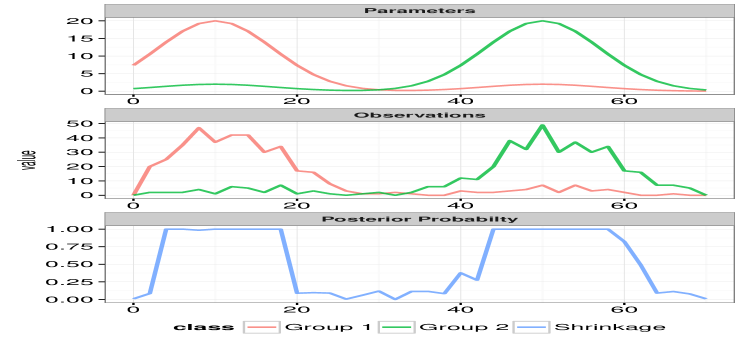
(a) $35$ equispaced points.

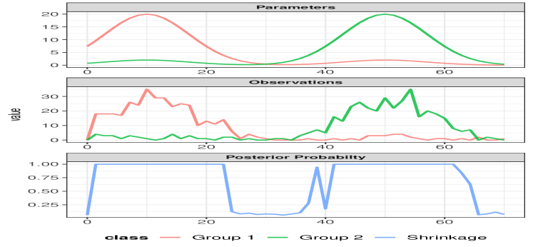
(b) $50$ equispaced points.

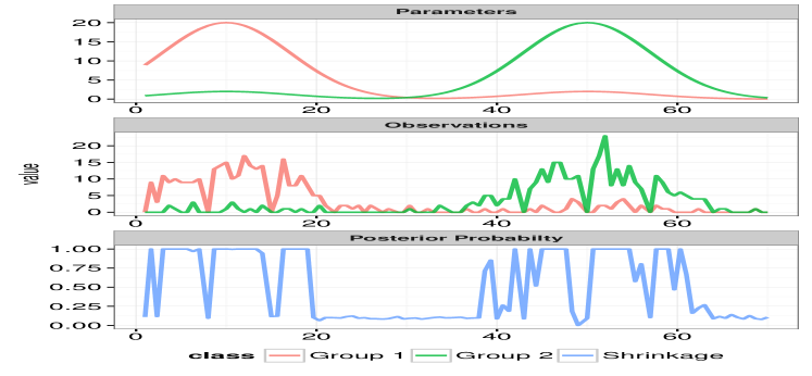
(c) $100$ equispaced points.

Figure 2: The posterior probabilities of difference in Poisson rate parameters $\omega_{i}=P(\lambda_{i,1}\neq\lambda_{i,2}|\mbox{data})$ along with true intensity functions and the observations generated.

Fig. 2(a) – 2(c) show the posterior probabilities of differential abundance $\omega_{i}$ along with the true intensity functions $\lambda_{1}(\cdot),\lambda_{2}(\cdot)$ and the counts ${\bf y}_{j}$s for the two partitions considered. The figures suggest that the posterior probabilities for differential abundance are close to $1$ near both the peaks where the intensity functions differ significantly, i.e. both between $[0,20]$ and $[40,60]$. Fig. 2(b) and Fig. 2(c) illustrate the behavior at finer scales by recovering sub-intervals of differential intensity at the cost of increased computation time. To gain efficiency, we can safely prune the region where the intensity functions are similar, making the posterior probability close to $0$, e.g. the interval $[20,35]$ as it cannot contain a differential sub-region at a finer scale. The CPU time (elapsed time in R) for the three resolutions were 26.47, 27.03, and 40.56 seconds, respectively, on a Dell Latitude 5310 with an Intel(R) Core(TM) i7-10810U CPU @ 1.10GHz. The R codes for replicating this simulation experiment can be found at https://github.com/DattaHub/twosampleDPM.

Although there does not exist a method that can be compared directly with our multiresolution-DPM model–either because they lack the multiresolution framework or the flexible nonparametric modeling part– it is possible to compare the DPM-Poisson model with a standard likelihood-ratio based test after suitable adjustment. To compare, we apply the poisson.test in R to the two count series obtained at $K=50$ resolutions and apply the Benjamini–Hochberg false discovery rate (FDR) control (Benjamini and Hochberg,, 1995), and apply the usual $FDR\leq 0.05$ cut-off for to the adjusted p-values. The positions of differential abundance thus identified are then compared with the posterior inclusion probabilities (PIP) along with a $0.5$ cut-off, corresponding to the median probability model (Barbieri and Berger,, 2004; Barbieri et al.,, 2021). Figure 3 shows the PIP versus p-values with FDR adjustment with overlaid binary series with the respective cut-offs: the methods agree on most parts, but the p-value based procedure leads to a missed discovery in the position $62.86$, with an adjusted p-value $0.0178$ and PIP of $0.794$. The results seem to suggest that the posterior inclusion probabilities $P(\lambda_{i,1}\neq\lambda_{i,2}|{\bf y}_{1},{\bf y}_{2})$ can be used for effectively controlling false discoveries without any further post hoc adjustment like the p-value based procedures, and the DPM-Poisson model is expected to be robust to the data-generating mechanism unlike the likelihood-ratio based tests. We would also like to note here that an analogous frequentist test, parametric or nonparametric, with such a multi-resolution structure could be developed that has such desirable properties.

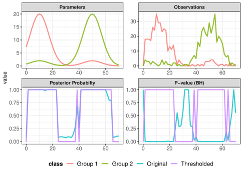
Figure 3: Comparison of pointwise exact test for two Poisson rates with the Benjamini–Hochberg FDR adjustment and the posterior inclusion probability obtained from the DPM-Poisson model in Fig. 1.

5 Application to Rare Variants Data

We apply our method to assess differences between the mutation rates for cases and controls based on rare variants data associated with common variable immunodeficiency (CVID). The background mutation rate for the control group is obtained from the Exome aggregation consortium (ExAC) that reports the total number of mutated alleles along the whole exome for 60,076 individuals. The observations represent rare variants ordered by their amino acid positions. We apply our method to the whole dataset and prune branches at each level based on the threshold for the probability of global null hypothesis restricted to each branch, and retain those that are likely to have at least one differentially mutated position. The successive levels are induced by the genes, the known protein domains within genes, and the amino acid positions within protein domains. If protein domain information is unavailable, one can grow the tree until sufficient data reduction has been achieved while keeping in mind that the probability of pruning a region with significant difference decreases with the number of levels of the tree.

We show the performance of our method with two protein-coding genes RAG2 and SNCAIP. RAG2 is involved in the development of B and T cells, and hyper-mutations on it have been associated with Omenn syndrome (Corneo et al.,, 2001). The exome sequencing data for $n=215$ CVID patients were collected in Dr. Sandeep Dave’s lab at Duke Medicine. We consider the publicly available ExAC database as a control for detecting regions on the gene where the mutation rates are different. The ExAC database reports the total number of mutated alleles or variants along the whole exome for $60,076$ healthy individuals, and provides information about genetic variation in the human population, and acts as a reliable source of background mutation rate. The number of mutated alleles for the CVID and the ExAC control group at the $i^{th}$ position are denoted by $Y_{i,1}$ and $Y_{i,2}$ respectively. We model $Y_{i,1}\sim\mbox{Poi}(N_{i1}\lambda_{i,1})$ and $Y_{i,2}\sim\mbox{Poi}(N_{i2}\lambda_{i,2})$ independently, where $\bm{\lambda}_{1}$, $\bm{\lambda}_{2}$ are the background mutation rates and $N_{i1},N_{i2}$ are the total number of alleles at position $i$ for the cases and controls respectively. We can fix these as $N_{i1}=N=2\times 60,076=120,152$, and $N_{i2}=N=2\times 215=430$ for our problem, but in general, the number of total alleles varies depending on a lot of factors, including sequencing depth. The mutation frequencies and the probabilities for differential abundance are plotted in Fig. 4(a) and Fig. 4(b).

Although it is difficult to assess whether the detected regions of hyper-mutation are truly associated with CVID without further study, the results concur with our expectations: 1) the multi-resolution tree prunes regions where the mutation rate in CVID cases is not higher than the background, as well as 2) the detected differential regions on RAG2 and SNCAIP fall in the known protein domain in the interval for amino acid positions. Our method also outperforms the scan-statistics approach by Ionita-Laza et al., (2012) on the same data set for detecting rare variants associated with CVID: the scan-statistics approach yields permutation P-values of $0.089$ and $0.034$ (based on $1,000$ permutations) for genes RAG2 and SNCAIP respectively for testing association of variants residing in the known protein domain, leading to ambiguity in inference. The scan statistics take longer time as expected, registering 131.01 and 164.37 seconds for the two genes RAG2 and SNCAIP for 1000 permutations, using the same computing resources as described in Section 4. In comparison, for our method, the CPU times recorded for the two genes RAG2 and SNCAIP were 63.52 and 95.68 seconds, respectively.

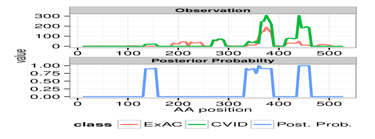
(a) RAG2

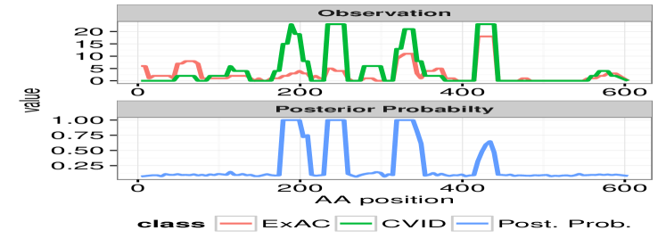
(b) SNCAIP

Figure 4: The performance of our method for detecting differences rare mutation rates between CVID cases and healthy controls on RAG2 and SNCAIP gene. The top and bottom pane shows the observed mutation data and the posterior probability of differential abundance respectively.

6 Conclusive remarks

We introduce a new multi-scale test of the difference between the rate of incidences between two groups, motivated by the problem of comparing rare variants profiles across two disease subtypes. The multi-resolution framework helps us substantially reduce the computational burden by focusing the search away from regions of no difference, informed by testing a composite null hypothesis. We use a Dirichlet process mixture of Poisson with Gamma base measure for modeling the intensity of each process with a spike-and-slab prior on differences. There are several future directions for this methodology and theory. Firstly, in many application areas such as environmental criminology, spatial data are aggregated to a pre-determined grid-level resolution for both response and predictor variables (Ek et al.,, 2023). A common feature in many of the models is that they combine geographic features such as built environments and socioeconomic variables at a chosen grid level over a geography. For example, the popular risk terrain modeling (RTM) (Caplan et al.,, 2011, 2015) creates a separate map layer for each predictor using a lattice grid of polygons, that are then combined to produce a composite map where the contribution or importance of each factor can be evaluated in a model-based way. Extending the multi-resolution Poisson-Gamma DPM for spatial data would be useful in such settings where spatial clustering or concentration of crime could aid in efficiency by the multi-resolution trimming approach. A second possible extension could be the use of shrinkage priors that could adapt to a broader range of sparsity, e.g., global-local priors for count data with quasi-sparsity such as the Gauss-hypergeometric (Datta and Dunson,, 2016) or extremely-heavy-tailed prior (Hamura et al.,, 2022). Finally, it would be interesting (from a purely theoretical viewpoint) to derive posterior contraction rates for the DPM-Poisson-Gamma model endowed with the two-groups test, similar to Ghosal et al., (1999). Finally, as pointed out by a referee, we believe that an extension to more than two groups is plausible within this framework, perhaps using a recursive scheme, depending on the context. For example, in genomics application, one could think of a baseline group and multiple disease sub-types and extend our DPM-Poisson model accordingly. Such an extension would be interesting to build but is currently out of scope for this manuscript.

Data Availability Statement

The exome sequencing data for CVID patients were collected in Dr. Sandeep Dave’s lab at Duke Medicine. The data are secondary, retrospective, and completely de-identified and are available from the authors on request.

References

- Agrawal et al., (1998) Agrawal, R., Gehrke, J., Gunopulos, D., and Raghavan, P. (1998). Automatic subspace clustering of high dimensional data for data mining applications.
- Anders and Huber, (2010) Anders, S. and Huber, W. (2010). Differential expression analysis for sequence count data. Genome biol, 11(10):R106.
- Barbieri and Berger, (2004) Barbieri, M. M. and Berger, J. O. (2004). Optimal predictive model selection. Annals of Statistics, pages 870–897.
- Barbieri et al., (2021) Barbieri, M. M., Berger, J. O., George, E. I., and Rovcková, V. (2021). The median probability model and correlated variables. Bayesian Analysis, 16(4):1085–1112.
- Benjamini and Hochberg, (1995) Benjamini, Y. and Hochberg, Y. (1995). Controlling the false discovery rate: a practical and powerful approach to multiple testing. Journal of the Royal statistical society: series B (Methodological), 57(1):289–300.
- Bogdan et al., (2011) Bogdan, M., Chakrabarti, A., Frommlet, F., and Ghosh, J. K. (2011). Asymptotic Bayes-optimality under sparsity of some multiple testing procedures. The Annals of Statistics, 39(3):1551–1579.
- Caplan et al., (2015) Caplan, J. M., Kennedy, L. W., Barnum, J. D., and Piza, E. L. (2015). Risk terrain modeling for spatial risk assessment. Cityscape, 17(1):7–16.
- Caplan et al., (2011) Caplan, J. M., Kennedy, L. W., and Miller, J. (2011). Risk terrain modeling: Brokering criminological theory and gis methods for crime forecasting. Justice Quarterly, 28(2):360–381.
- Corneo et al., (2001) Corneo, B., Moshous, D., Güngör, T., Wulffraat, N., Philippet, P., Le Deist, F., Fischer, A., and de Villartay, J.-P. (2001). Identical mutations in rag1 or rag2 genes leading to defective v (d) j recombinase activity can cause either tb–severe combined immune deficiency or omenn syndrome. Blood, 97(9):2772–2776.
- Datta and Dunson, (2016) Datta, J. and Dunson, D. B. (2016). Bayesian inference on quasi-sparse count data. Biometrika, 103(4):971–983.
- Dhavala et al., (2010) Dhavala, S. S., Datta, S., Mallick, B. K., Carroll, R. J., Khare, S., Lawhon, S. D., and Adams, L. G. (2010). Bayesian modeling of mpss data: gene expression analysis of bovine salmonella infection. Journal of the American Statistical Association, 105(491):956–967.
- Ek et al., (2023) Ek, A., Drawve, G., Robinson, S., and Datta, J. (2023). Quantifying the effect of socio-economic predictors and the built environment on mental health events in Little Rock, AR. ISPRS International Journal of Geo-Information, 12(5):205.
- Fier et al., (2012) Fier, H., Won, S., Prokopenko, D., AlChawa, T., Ludwig, K. U., Fimmers, R., Silverman, E. K., Pagano, M., Mangold, E., and Lange, C. (2012). ‘Location, Location, Location’: a spatial approach for rare variant analysis and an application to a study on non-syndromic cleft lip with or without cleft palate. Bioinformatics, 28(23):3027–3033.
- Ghosal et al., (1999) Ghosal, S., Ghosh, J. K., and Ramamoorthi, R. (1999). Posterior consistency of Dirichlet mixtures in density estimation. The Annals of Statistics, 27(1):143–158.
- Guindani et al., (2014) Guindani, M., Sepúlveda, N., Paulino, C. D., and Müller, P. (2014). A Bayesian semiparametric approach for the differential analysis of sequence counts data. Journal of the Royal Statistical Society: Series C (Applied Statistics), 63(3):385–404.
- Hamura et al., (2022) Hamura, Y., Irie, K., and Sugasawa, S. (2022). On global-local shrinkage priors for count data. Bayesian Analysis, 17(2):545–564.
- Hardcastle and Kelly, (2010) Hardcastle, T. J. and Kelly, K. A. (2010). bayseq: empirical bayesian methods for identifying differential expression in sequence count data. BMC bioinformatics, 11:1–14.
- Ionita-Laza et al., (2012) Ionita-Laza, I., Makarov, V., Buxbaum, J. D., Consortium, A. A. S., et al. (2012). Scan-statistic approach identifies clusters of rare disease variants in LRP2, a gene linked and associated with autism spectrum disorders, in three datasets. The American Journal of Human Genetics, 90(6):1002–1013.
- Kulldorff, (1997) Kulldorff, M. (1997). A spatial scan statistic. Communications in Statistics-Theory and methods, 26(6):1481–1496.
- Li and Leal, (2008) Li, B. and Leal, S. M. (2008). Methods for detecting associations with rare variants for common diseases: application to analysis of sequence data. The American Journal of Human Genetics, 83(3):311–321.
- Lin and Tang, (2011) Lin, D.-Y. and Tang, Z.-Z. (2011). A general framework for detecting disease associations with rare variants in sequencing studies. The American Journal of Human Genetics, 89(3):354–367.
- McAuliffe et al., (2006) McAuliffe, J. D., Blei, D. M., and Jordan, M. I. (2006). Nonparametric empirical Bayes for the Dirichlet process mixture model. Statistics and Computing, 16(1):5–14.
- Meng et al., (2020) Meng, J., Zhu, W., Li, C., and Jon, K. (2020). A novel association test for rare variants based on algebraic statistics. Journal of Theoretical Biology, 493:110228.
- Morgenthaler and Thilly, (2007) Morgenthaler, S. and Thilly, W. G. (2007). A strategy to discover genes that carry multi-allelic or mono-allelic risk for common diseases: a cohort allelic sums test (cast). Mutation Research/Fundamental and Molecular Mechanisms of Mutagenesis, 615(1):28–56.
- Neill et al., (2004) Neill, D., Moore, A., Pereira, F., and Mitchell, T. M. (2004). Detecting significant multidimensional spatial clusters. Advances in Neural Information Processing Systems, 17.
- Neill and Moore, (2004) Neill, D. B. and Moore, A. W. (2004). A fast multi-resolution method for detection of significant spatial disease clusters. In Advances in Neural Information Processing Systems, pages 651–658.
- Nicolae, (2016) Nicolae, D. L. (2016). Association tests for rare variants. Annual review of genomics and human genetics, 17:117–130.
- Nie et al., (2006) Nie, L., Wu, G., Brockman, F. J., and Zhang, W. (2006). Integrated analysis of transcriptomic and proteomic data of desulfovibrio vulgaris: zero-inflated poisson regression models to predict abundance of undetected proteins. Bioinformatics, 22(13):1641–1647.
- Pritchard, (2001) Pritchard, J. K. (2001). Are rare variants responsible for susceptibility to complex diseases? The American Journal of Human Genetics, 69(1):124–137.
- Rempala et al., (2011) Rempala, G. A., Seweryn, M., and Ignatowicz, L. (2011). Model for comparative analysis of antigen receptor repertoires. Journal of theoretical biology, 269(1):1–15.
- Robinson et al., (2010) Robinson, M. D., McCarthy, D. J., and Smyth, G. K. (2010). edgeR: a Bioconductor package for differential expression analysis of digital gene expression data. BMC Bioinformatics, 26(1):139–140.
- Sepúlveda et al., (2010) Sepúlveda, N., Paulino, C. D., and Carneiro, J. (2010). Estimation of t-cell repertoire diversity and clonal size distribution by poisson abundance models. Journal of immunological methods, 353(1-2):124–137.
- Shayesteh et al., (1999) Shayesteh, L., Lu, Y., Kuo, W.-L., Baldocchi, R., Godfrey, T., Collins, C., Pinkel, D., Powell, B., Mills, G. B., and Gray, J. W. (1999). PIK3CA is implicated as an oncogene in ovarian cancer. Nature Genetics, 21(1):99–102.
- Thygesen and Zwinderman, (2006) Thygesen, H. H. and Zwinderman, A. H. (2006). Modeling sage data with a truncated gamma-poisson model. BMC bioinformatics, 7:1–9.
- Trippa and Parmigiani, (2011) Trippa, L. and Parmigiani, G. (2011). False discovery rates in somatic mutation studies of cancer. The Annals of Applied Statistics, pages 1360–1378.
- van Dokkum et al., (2020) van Dokkum, P., Lokhorst, D., Danieli, S., Li, J., Merritt, A., Abraham, R., Gilhuly, C., Greco, J. P., and Liu, Q. (2020). Multi-resolution filtering. Publications of the Astronomical Society of the Pacific, 132(1013):1–17.
- Wu et al., (2011) Wu, M. C., Lee, S., Cai, T., Li, Y., Boehnke, M., and Lin, X. (2011). Rare-variant association testing for sequencing data with the sequence kernel association test. The American Journal of Human Genetics, 89(1):82–93.
- Zuyderduyn, (2007) Zuyderduyn, S. D. (2007). Statistical analysis and significance testing of serial analysis of gene expression data using a Poisson mixture model. BMC Bioinformatics, 8(1):1.