Interpretation of near-threshold peaks using the method of independent S-matrix poles

Abstract

We propose a model-independent analysis of near-threshold enhancements using independent S-matrix poles. In this formulation, we constructed a Jost function with controllable zeros to ensure that no poles are generated on the physical Riemann sheet. We show that there is a possibility of misinterpreting the observed near-threshold signals if one utilized a limited parametrization and restrict the analysis to only one element of the S-matrix. Specifically, there is a possibility of the emergence of ambiguous pair of poles which are singularities of the full S-matrix but may not manifest in one of its elements. For a more concrete discussion, we focused on an effective two-channel scattering where the full S-matrix is a $2\times 2$ matrix. We apply our method to the coupled two-channel analysis of the $P_{\psi}^{N}(4312)^{+}$ and found that the compact pentaquark interpretation cannot be ruled out yet.

I Introduction

One of the active areas of investigation in hadron spectroscopy is the interpretation of near-threshold phenomena Olsen et al. (2018); Guo et al. (2018); Oller (2020); Guo et al. (2020); Mai et al. (2023); Albaladejo et al. (2022). In 2019, an updated analysis of the $\Lambda^{0}_{b}\to J/\psi pK^{-}$ decays based on Runs 1 and 2 of the LHCb collaboration was presented in Ref. Aaij et al. (2019). They observed the narrow pentaquark state $P_{\psi}^{N}(4312)^{+}$ (then called the $P_{c}(4312)^{+}$) together with the two-peak structure of the $P_{c}(4450)^{+}$ resonance which was not present in their initial analysis in Ref. Aaij et al. (2015). These newly observed resonances have narrow decay widths and are below the $\Sigma_{c}\bar{D}$ or $\Sigma_{c}\bar{D}^{*}$, a typical signature of molecules. Ref. Aaij et al. (2019) had concluded that $P_{\psi}^{N}(4312)^{+}$ is a virtual state with the $\Sigma^{+}_{c}\bar{D}^{0}$ threshold being within its extent. A similar parametrization study Ref. Fernández-Ramírez et al. (2019) and a deep learning approach Ref. Ng et al. (2022) had the same conclusion for the $P_{\psi}^{N}(4312)^{+}$ signal.

Other interpretations are possible and were done in different studies. For example, in Ref. Chen et al. (2019) the $P_{\psi}^{N}(4312)^{+}$ resonance is favored to have a molecular structure using the QCD sum rules formalism. It was found to be the $[\Sigma_{c}^{++}\bar{D}^{-}]$ bound state with $J^{P}=1/2^{-}$. The molecular picture and same quantum number is favored as well in Ref. Cheng and Liu (2019) where they studied the mass and decay properties of $P_{\psi}^{N}(4312)^{+}$ using isospin breaking effects and rearrangement decay properties. Ref. Du et al. (2020) used a coupled-channel formalism and ends up with the same conclusion.

In Ref. Matuschek et al. (2021), it was argued that if range corrections can be neglected, virtual states are molecular in nature and hence the studies cited above poses no contradiction. As can be observed, the molecular picture is favored by most studies. However, we still cannot dismiss the compact pentaquark picture since information about quantum numbers and decay properties is lacking experimentally. In fact a model based approach in Ref. Ali and Parkhomenko (2019), the resonance was studied under the compact diquark model as a hidden-charm diquark-diquark-antiquark baryon with $J^{P}=3/2^{+}$.

Until we settle the quantum numbers and decay properties of the $P_{c}$ resonances of the $\Lambda_{b}^{0}\to J/\psi pK^{-}$, we cannot completely rule out the compact nature of the $P_{\psi}^{N}(4312)^{+}$. A good way to investigate this resonance with some of its properties still ambiguous is by using a minimally biased bottom-up approach study Albaladejo et al. (2022). The $S$-matrix is a good tool to use in a bottom-up approach study as it can be constructed without any details of the interacting potential. We only need to impose analyticity, and hermiticity and unitarity below the first threshold. Given these three mathematical restrictions, we can reproduce the scattering amplitude from experiment by identifying the optimal placement and number of poles in the scattering process. Finally, we can look for a theoretical model that can reproduce the same analytic properties of the constructed $S$-matrix.

In this paper, we show that some arrangements of poles may not be accommodated by the usual amplitude parametrizations such as the effective range expansion. Specifically, there are combinations of poles which will not manifest in the line shape of the elastic scattering amplitude. This, in turn, opens up the possibility of having a pole structure that caters the compact nature of $P_{\psi}^{N}(4312)^{+}$. The difficulty of capturing these subtle pole configurations may arise due to the contamination of coupled channel effects. For example, a weakly interacting final state hadrons (higher mass channel) may have a virtual state pole that can be displaced away from the real energy axis due to coupling with the lower mass channel. If there is a resonance that is strongly coupled to the lower mass channel, then the displaced virtual state pole and the shadow pole of the resonance may have a cancellation effect in the elastic transition amplitude. One can invoke the pole-counting method to interpret a near-threshold pole with an accompanying shadow pole as non-molecular Morgan (1992); Morgan and Pennington (1991, 1993). In this work, we propose to use the independent S-matrix poles to accommodate all possible interpretations of the observed near-threshold enhancements.

The content of this paper is organized as follows: In section II, we review the formalism of the $S$-matrix and show how one can construct an S-matrix using independent poles via the uniformization scheme introduced in Refs. Newton (1982); Kato (1965); Yamada and Morimatsu (2020, 2021); Yamada et al. (2022). In section III, we discuss how identical line shapes arises. We show that the ambiguity can be resolved by adding the contribution of the off diagonal $T_{21}$ channel. As an application, we investigate the $P_{\psi}^{N}(4312)^{+}$ signal and show that its $T_{11}$ line shape can take a $1$-pole configuration or $3$-pole configuration. In section IV, we give our conclusion and outlook for future works.

II Formalism

The $S$-matrix is an operator that describes the interaction of a scattering process. In momentum space, one could decompose the $S$-matrix in terms of the non-interacting terms and interacting terms as Taylor (1972)

$$\bra{\mathbf{p^{\prime}}}S\ket{\mathbf{p}}=\delta^{3}(\mathbf{p^{\prime}}-\mathbf{p})+\frac{i}{2\pi m}\delta(E_{p^{\prime}}-E_{p})f(\mathbf{p^{\prime}}\leftarrow\mathbf{p})$$ (1)

where $f(\mathbf{p^{\prime}}\leftarrow\mathbf{p})$ is the scattering amplitude from momentum $\mathbf{p}$ to $\mathbf{p^{\prime}}$ and the factors of the interacting term may vary depending on the literature. The scattering amplitude $f(\mathbf{p^{\prime}}\leftarrow\mathbf{p})$ is related to the cross section via

$$\frac{\mathrm{d}\sigma}{\mathrm{d}\Omega}(\mathbf{p}\leftarrow\mathbf{p_{0}})=|f(\mathbf{p}\leftarrow\mathbf{p_{0}})|^{2}.$$ (2)

In principle, we could use equations (1) and (2) to construct a parametrized $S$-matrix to fit it in the measured cross section data from experiments. The peaks from such data are characterized by the pole singularities of the $S$-matrix and it is indicative of the nature of the intermediate particles.

In practice, the usual treatment of peaks in the scattering cross section is to utilize the Breit-Wigner parametrization to extract the mass and width of the resonance. This approach works very well if the peaks are far from any threshold and the widths are narrow. However, most of the recently observed peaks occur very close to some two-hadron threshold, where the peaks are no longer a reliable information to quote the mass of the observed state. Moreover, coupled-channel effects can no longer be ignored if the peaks are close to the thresholds. Unlike the complex energy plane of a single-channel system, one has to probe deeper into the multiple Riemann sheets of the energy complex plane of a multi-channel scattering. Specifically, the peaks observed may correspond to different pole arrangements in different Riemann sheets.

In a one-channel scattering, we are interested in singularities of the complex momentum $p$ - plane. The poles on its positive imaginary axis correspond to bound states and the poles below its real axis may correspond to resonances. With the relativistic energy-momentum relation $p^{\mu}p_{\mu}=E^{2}-\vec{p}\cdot\vec{p}=m^{2}$, the complex momentum $p$-plane transforms into two Riemann sheets of the complex energy $E$. The first Riemann sheet (top sheet) of $E$, which we call the physical sheet, corresponds to the upper half plane of $p$. The importance of physical sheet is that the scattering region lies on this complex energy plane. The scattering region corresponds to the energy axis used in plotting scattering observables. The second Riemann sheet (bottom sheet) of $E$, which we call the unphysical sheet, corresponds to the lower half plane of $p$. Due to causality, no other singularities should be present in the physical energy sheet aside from bound state poles and a branch point at the threshold van Kampen (1953a, b).

Accordingly, in a two-channel scattering, we get four Riemann sheets (see Rakityansky (2022) for an in-depth discussion). Only poles closest to the scattering region are relevant in the description of scattering data. In this paper, we used the notation of Pearce and Gibson in Pearce and Gibson (1989) in labeling our Riemann sheets. We label the sheets as $[XY]$ where the string can be $t$ or $b$ to denote a top sheet or bottom sheet and the order of character denotes the channel. For example. the sheet $[bt]$ corresponds to the bottom sheet of the first channel and top sheet of the second channel. The correspondence of Pearce and Gibson’s notation with the more commonly used notation of Frazer and Hendry Frazer and Hendry (1964) is listed in Table 1.

Frazer and Hendry	Pearce and Gibson	Topology in complex $E$
I	$[tt]$	$\theta_{1}\in(0,2\pi)$; $\theta_{2}\in(0,2\pi)$
II	$[bt]$	$\theta_{1}\in(2\pi,4\pi)$; $\theta_{2}\in(0,2\pi)$
III	$[bb]$	$\theta_{1}\in(2\pi,4\pi)$; $\theta_{2}\in(2\pi,4\pi)$
IV	$[tb]$	$\theta_{1}\in(0,2\pi)$; $\theta_{2}\in(2\pi,4\pi)$

Table 1: Riemann sheet notation. In this work, we will follow Pearce and Gibson’s notation. The index correspond to the channel number and $t(b)$ denotes top(bottom) sheet.

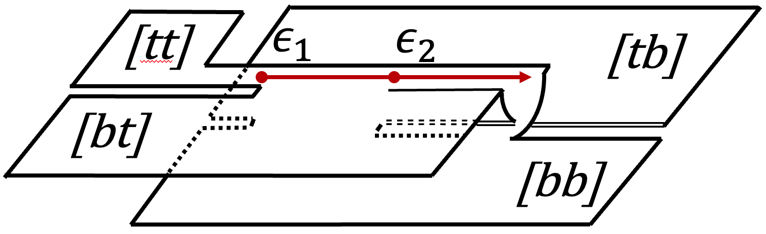
(a)

(b)

Figure 1: The relevant regions of the four Riemann sheets in a two-channel scattering. (a) The energy complex plane. (b) The uniformized variable $\omega$ plane mapped from the complex energy $E$-plane using uniformization.

We show in Figure 1(a) an illustration of the four Riemann sheets in a two-channel scattering. The scattering region is represented by the red ray with two dots (branch points) lying on the physical sheet $[tt]$. It is directly connected with the lower halves of the $[bt]$ and $[bb]$ sheets. Crossing the branch cut between the first energy threshold $\epsilon_{1}$ and second energy threshold $\epsilon_{2}$, will send us to the $[bt]$ sheet. On the other hand, if we cross the branch cut above $\epsilon_{2}$, we end up in the $[bb]$ sheet. Energy poles found on these two sheets are quoted with negative imaginary parts. Consequently, these poles fit the description of unstable quantum states since their negative imaginary parts can reproduce the expected exponential decay of unstable states. On the other hand, energy poles on the $[tb]$ sheet are quoted with positive imaginary parts since only the upper half plane of the $[tb]$ sheet affect the scattering region. This gives rise to an exponential increase in time which does not correspond to any quantum state.

II.1 Analytic Structure of a two-channel S-matrix

Without loss of generality, we can focus on an effective two-channel scattering. The full two-channel transition is described by a $2\times 2$ $S$-matrix whose elements are given by

$$S_{11}(p_{1},p_{2}) =\dfrac{D(-p_{1},p_{2})}{D(p_{1},p_{2})};\quad S_{22}(p_{1},p_{2})=\dfrac{D(p_{1},-p_{2})}{D(p_{1},p_{2})}$$ (3)

and

$$S_{12}^{2}=S_{11}S_{22}-\text{det}S$$ (4)

where $D(p_{1},p_{2})$ is the Jost function Couteur (1960); Newton (1961, 1962). The subscripts correspond to the channel index with $1$ representing the lower mass channel, and $2$ for the higher mass. Causality requires that the $S$-matrix be analytic up to the branch points and poles van Kampen (1953b, a). These singularities are related to the details of scattering. Branch cuts are dictated by kinematics while the poles are dynamical in nature. Depending on the location of the pole on the Riemann sheet, it may in general correspond to a bound state, virtual state or resonance Badalyan et al. (1982). The zeros of the Jost function $D(p_{1},p_{2})$ correspond to the poles of the S-matrix. Analyticity is imposed on (3) by requiring $\lim_{|p_{1}|,|p_{2}|\to\infty}D(p_{1},p_{2})=1$ for $\text{Im}\ p_{n}\geq 0$ Newton (1982, 1961). The Schwarz reflection principle and the hermiticity of the S-matrix below the lowest threshold ensures that for every momentum pole $\bar{p_{i}}$, there is another pole given by $-\bar{p_{i}}^{*}$. All of these must be considered in the construction of the Jost function.

From equation (3), we see that the $S$-matrix is a ratio of two Jost functions. One of the most straightforward ways to construct an analytic, unitary, and symmetric $S$-matrix is by using a Jost function, of the form $D\propto p^{-N}\sum_{n}^{N}\alpha_{n}p^{n}$ where $p=\{p_{1},p_{2}\}$. The extra factor $p^{-N}$ is needed to ensure that as $|p|\rightarrow\infty$ we get $D\rightarrow 1$. The polynomial part, when written in factored form, allows us to form a set of independent zeros of $D(p_{1},p_{2})$.

II.2 Independent poles via uniformization scheme

We propose the use of independent poles in the analysis of near-threshold signals for two reasons. First, this is to ensure that the treatment is model-independent. In other parametrizations, such as the Flatté or effective range expansion, fixing one of the poles will necessarily alter the position of the other pole. These parametrizations may be constructed without reference to any models but one can always find an effective coupled-channel potential that can reproduce such pole trajectory Pearce and Gibson (1989); Frazer and Hendry (1964); Hanhart et al. (2014); Hyodo (2014). Second, a parametrization that allows independence of poles can cover a wider model space without violating the expected properties of the S-matrix unlike in other parametrization. This limitation is observed in Frazer and Hendry (1964) where a specific coupled-channel effective range approximation can only produce poles in either $[bt]$ or $[tb]$ sheet but not in $[bb]$. An S-matrix with independent poles can cover a wider model space without compromising any of the expected properties of S-matrix.

It is also important that the amplitude model to be used gives the correct threshold behavior associated with branch point singularity of the two-hadron scattering. The uniformization method introduced in Kato (1965); Newton (1982) and utilized in Yamada and Morimatsu (2021, 2020) is an appropriate scheme for our present objective. The $k$th channel’s momentum in the two-hadron center of mass frame is given by

$$p_{k}^{2}=\dfrac{(s-\epsilon_{k}^{2})\left[s-\epsilon_{k}(\epsilon_{k}-4\mu_{k})\right]}{4s}$$ (5)

where $\epsilon_{k}$ is the threshold energy and $\mu_{k}$ is the reduced mass of the system. The invariant Mandelstam variable $s$ is can be written as

$$s=\epsilon_{k}^{2}+\dfrac{\epsilon_{k}}{\mu_{k}}|\vec{p}_{k}|^{2}\left[1+\mathcal{O}\left(\dfrac{|\vec{p}_{k}|^{2}}{\epsilon_{k}^{2}}\right)\right]=\epsilon_{k}^{2}+q_{k}^{2}.$$ (6)

where we introduced the new momentum variable $q_{k}$ for convenience of scaling.

Instead of constructing the $S$-matrix using the momenta $q_{1}$ and $q_{2}$, we introduce the uniformized variable $\omega$ defined by the transformation

$$\omega=\dfrac{q_{1}+q_{2}}{\sqrt{\epsilon_{2}^{2}-\epsilon_{1}^{2}}};\quad\quad\dfrac{1}{\omega}=\dfrac{q_{1}-q_{2}}{\sqrt{\epsilon_{2}^{2}-\epsilon_{1}^{2}}}.$$ (7)

The linear dependence of the $\omega$ with $(q_{1},q_{2})$ removes the issue of branch point singularity associated with the threshold. In other words, uniformization reduces the number of complex planes from four energy planes to only one $\omega$ plane. Figure 1(b) shows the $\omega$ - plane and a detailed description of such mapping can be seen in Kato (1965); Yamada et al. (2022). All the relevant halves of the complex energy planes in Fig. 1(a) are on the 1st and 4th quadrants of the $\omega$ plane in Fig. 1(b).

Referring to equations (3) and (4), we can use a rational Jost function $D(\omega)$ such that the pole of the $S$-matrix is easily determined by its zeros. The simplest Jost function takes the form

$$D(\omega)=\dfrac{1}{\omega^{2}}(\omega-\omega_{\text{pole}})(\omega+\omega_{\text{pole}}^{*})(\omega-\omega_{\text{reg}})(\omega+\omega_{\text{reg}}^{*})$$ (8)

where we had introduced several factors. The negative conjugate terms are a consequence of the hermiticity of the $S$-matrix below the lowest threshold Yamada and Morimatsu (2020); Taylor (1972). The extra pole $\omega_{\text{reg}}$, called the regulator, is added to ensure that the $k$th diagonal elements of the S-matrix behave as $S_{kk}(\omega)\rightarrow 1$ as $\omega\rightarrow\infty$ Kato (1965); Newton (1982). In the short-ranged potential scattering theory, we expect the phase shift to vanish at large energies to be consistent with the Levinson’s theorem. This expectation can be met when we impose $|\omega_{reg}\omega_{\text{pole}}|=1$. This means that we have another pole which depend on $\omega_{\text{pole}}$. To ensure that $\omega_{\text{pole}}$ is the only relevant pole that can affect the interpretation of enhancement, we set the regulator to be far from the scattering region. Referring to the uniformized $\omega$ plane in Fig. 1(b), one can minimize the influence of the regulator by placing it either on the $[bb]$ or the $[tb]$ sheet. Note that a regulator pole on the $[bt]$ sheet will result into a structure between the two thresholds, which significantly affects the interpretation of the line shape, hence it is in our best interest to avoid putting a regulator in this region. The simplest regulator we could use following these requirements is $\omega_{\text{reg}}=e^{-i\pi/2}/|\omega_{\text{pole}}|$, where the phase factor ensures that the regulator falls on either the $[tb]$ or $[bb]$ sheet below the lowest threshold.

We reiterate the importance of regulator not affecting the physics of the $S$-matrix. In Yamada and Morimatsu (2020), the uniformized truncated Mittag-Leffler parametrization neglected the $\omega_{\text{reg}}$ regulator. Such formulation assumes that the conjugate pole $\omega_{\text{pole}}^{*}$ is much closer to the scattering region than the $\omega_{\text{reg}}$. The absence of other background poles, especially $\omega_{\text{reg}}$, makes the contribution of $\omega_{\text{pole}}^{*}$ relevant in the interpretation of the $\Lambda(1405)$, which resulted into a broad line shape in the $\pi\Sigma$ mass distribution. This is the reason why the authors of Yamada and Morimatsu (2020) concluded that the $\Lambda(1405)$ requires only one pole in the second Riemann sheet in contrast with the current consensus of two-pole structure interpretation Workman et al. (2022); Wang et al. (2021); Meißner (2020); Hyodo and Jido (2012). Care must be taken in the construction of amplitudes. Removing the contribution of $\omega_{\text{reg}}$, or any possible background poles, as emphasized in Kato (1965) might lead into misinterpretation of line shapes.

In other parametrizations, such as the K-matrix model (see for example Kuang et al. (2020)), the equation for the poles are typically quartic in the channel momenta. One may set the Riemann sheet of the desired relevant pole by adjusting the coupling parameters but there is always a tendency that a shadow pole will appear on the physical sheet Sombillo et al. (2021a); Eden and Taylor (1964). The linear dependence of the uniformized variable $\omega$ on the channel momenta in Eq.(7) guarantees that no shadow pole is produced using the Jost function in (8). The regulator pole, which can be controlled in our formulation, ensured that the S-matrix will not violate causality. In situation where there is an actual shadow pole, an independent pole can be added to the Jost function with no direct relation to the main pole. That is, one can freely place the pole and its shadow in any position without being restricted by some coupling parameter. With all of these considerations, the full Jost function with different combinations of $N$ independent poles takes the form:

$$D(\omega)=\dfrac{1}{\omega^{2N}}\prod_{\{\text{pole, reg}\}}^{N}(\omega-\omega_{\text{pole}})(\omega+\omega_{\text{pole}}^{*})(\omega-\omega_{\text{reg}})(\omega+\omega_{\text{reg}}^{*}).$$ (9)

Using the independent-pole form of the Jost function in Eq.(9), the two-channel S-matrix elements satisfying unitarity, analyticity, and hermiticity below the lowest threshold takes the form

$$S_{11}(\omega)=\dfrac{D(-1/\omega)}{D(\omega)};\quad S_{22}(\omega)=\dfrac{D(1/\omega)}{D(\omega)};\quad\text{det}(S)=\dfrac{D(-\omega)}{D(\omega)}.$$ (10)

The scattering amplitude $T_{j,k}(\omega)$ can be obtained from the relation $S_{j,k}=\delta_{j,k}-2iT_{j,k}$ where $\delta_{j,k}$ is the Kronecker delta.

III Ambiguous line shapes

The independent poles of the full S-matrix are determined by the zeros of the $D(\omega)$. It is possible that the zero of denominator cancels the zero of the numerator for one of the S-matrix element, say $S_{11}$. This means that such pole will not manifest in the line shape as if it did not exist at all. This subtle features of the S-matrix is important as we can potentially miss out other possible pole configurations if we probe only one element of the full $S$-matrix. In this section, we first present on how this ambiguity arises. We emphasize that this ambiguity is dependent on the parametrization of the $S$-matrix. In particular, the ambiguity of the formalism we use arises from the parametrization of the regulator. As an application, we discuss the implication of the ambiguous line shapes in the context of the $P_{\psi}^{N}(4312)^{+}$ signal. We propose that such ambiguity can be removed by probing the off diagonal term of the $S$-matrix. We close the section by discussing the importance of probing the off diagonal $S$-matrix terms and the limitation of the effective range expansion.

III.1 Emergence of ambiguity

Here, we point out that there exists a pole configuration that has no effect on one of the elements of the full S-matrix. We start by looking at the pole configuration of one of the $S$-matrix element that is equal to unity. We focus on the ambiguity of the $S_{11}$ channel. Recall that we construct the $S_{11}(\omega)$ element as

$$\begin{split}S_{11}(\omega)&=\frac{D(-1/\omega)}{D(\omega)}\\ &=\omega^{4N}\frac{\prod_{\{\text{zero,reg}\}}^{N}(-1/\omega-\omega_{\text{zero}})(-1/\omega-\omega_{\text{reg}})(-1/\omega+\omega_{\text{zero}}^{*})(-1/\omega+\omega_{\text{reg}}^{*})}{\prod_{\{\text{pole,reg}\}}^{N}(\omega-\omega_{\text{pole}})(\omega-\omega_{\text{reg}})(\omega+\omega_{\text{pole}}^{*})(\omega+\omega_{\text{reg}}^{*})}\\ &=\omega^{4N}\frac{\prod_{\{\text{zero,reg}\}}^{N}(-1/\omega-\omega_{\text{zero}})\times(\text{reg.})\times(-\text{c.c})}{\prod_{\{\text{pole,reg}\}}^{N}(\omega-\omega_{\text{pole}})\times(\text{reg.})\times(-\text{c.c})}\end{split}$$ (11)

where the notation in the last line is introduced for convenience. The terms reg. and c.c. denote the regulator and complex conjugate of the zeros (or poles) of the preceding terms, respectively. With some foresight, we consider the pair of poles $\omega_{\text{pole 1}}=a$ and $\omega_{\text{pole 2}}=-1/a$. From (11), the $S_{11}(\omega)$ matrix element reads as

$$\begin{split}S_{11}(\omega)&=\omega^{8}\times\frac{(-1/\omega-a)}{(\omega-a)}\cdot\frac{(-1/\omega+1/a)}{(\omega+1/a)}\times(\text{reg})\times(-\text{c.c.})\\ &=\omega^{8}\times\left(-\frac{1}{\omega^{2}}\right)\times\left(-\frac{1}{\omega^{2}}\right)\times\left(\frac{1}{\omega^{4}}\right)\\ &=1\end{split}$$ (12)

The pair of poles $\omega_{\text{pole 1}}=a$ and $\omega_{\text{pole 2}}=-1/a$ entails a unitary $S$-matrix. We will call such combination of poles that lead to a unitary $S$-matrix element as “ambiguous pair poles.” In terms of momentum, recalling equation (7), the pair poles $\omega_{\text{pole 1}}=a$ and $\omega_{\text{pole 2}}=-1/a$ translates into

$$\frac{q_{1}^{(2)}+q_{2}^{(2)}}{\sqrt{\epsilon_{2}^{2}-\epsilon_{1}^{2}}}=\frac{q_{2}^{(1)}-q_{1}^{(1)}}{\sqrt{\epsilon_{2}^{2}-\epsilon_{1}^{2}}}$$ (13)

where $q_{n}^{(m)}$ denotes the momentum of the $n$th channel of the $m$th pole. It follows from (13) that $q_{1}^{(2)}+q_{1}^{(1)}=0$ for the equation to hold; the takeaway is that the imaginary part of the $q_{1}$ pair must be opposite. This implies that the pair poles should either be found separately on the $[tt]$ and $[bt]$ sheet or on the $[bb]$ and $[tb]$ sheets. The former instance is prohibited since it will violate analyticity and causality. Hence, we consider two poles in which one is located at the $[tb]$ sheet and the other at the $[bb]$ sheet an ambiguous pair pole if $\omega_{\text{pole}[tb]}\omega_{\text{pole}[bb]}=-1$. Moreover, their regulators are given by $\omega_{\text{reg of $[bb]$ pole}}=-ia$ and $\omega_{\text{reg of $[tb]$ pole}}=i/a$, located on the $[tb]$ and $[bb]$ sheets, respectively.

The condition for the ambiguous pair poles states no specific magnitude for it to occur, only that they must depend on each other as $\omega_{\text{pole}[tb]}\omega_{\text{pole}[bb]}=-1$. Despite that these ambiguous pair poles have no effective contribution in the $T_{11}$ line shape, they cannot be ignored especially when they are near the threshold. If we probe either the $T_{12}$ or $T_{22}$ channel, we will observe a difference between the two configurations. We then assert that one must be rigorous in using certain approximations. For example, without proper justification, the prescription $\mathrm{d}N/\mathrm{d}\sqrt{s}\propto|T_{11}|^{2}$ might potentially miss out pole configurations with ambiguous pair poles.

Through a similar argument, we could assert that the same conclusion holds for the $S_{22}$ channel. The ambiguous pair for the $S_{22}$ channel should lie on the $[bb]$ and $[bt]$ sheet and satisfies $\omega_{\text{pole}[bt]}\omega_{\text{pole}[bb]}=1$. However, this will only be possible if we reassign the regulator of the pole at the $[bt]$ sheet as $\omega_{\text{reg of $[bt]$}}=e^{i\pi/2}/|\omega_{\text{pole in $[bt]$}}|$, i.e., the regulator should be placed on the $[tt]$ sheet instead of the $[bb]$ sheet. We consider for a moment this pole on the $[bt]$ sheet and its regulator. Recalling equations (9) and (10), we have

$$S_{22}=\omega^{4}\frac{(1/\omega-\omega_{[bt]})(1/\omega+\omega_{[bt]}^{*})}{(\omega-\omega_{[bt]})(\omega+\omega_{[bt]}^{*})}\cdot\frac{(1/\omega-\omega_{[tt]})(1/\omega+\omega_{[tt]}^{*})}{(\omega-\omega_{[tt]})(\omega+\omega_{[tt]}^{*})}$$ (14)

where the second fraction are the regulator terms and its complex conjugates. Since $\omega_{tt}$ is located at the imaginary axis, the denominator of the second fraction is equal to $(\omega-\omega_{[tt]})^{2}$, which makes the singularity a double pole. We have to recall that state correspondence is always a simple pole Newton (1982); Taylor (1972) and hence, our regulator assignment on the $[tt]$ sheet does not invalidate causality. Moreover, this 2nd order $[tt]$ pole is faraway from the threshold, and hence its presence is not relevant in the interpretation of amplitude line shape.

III.2 Implication of the ambiguous line shapes

To demonstrate the ambiguous line shape and its consequences, we look into the LHCb $P^{N}_{\psi}(4312)^{+}$ signal. We reconstruct its scattering amplitude using the data and best fit found in Fernández-Ramírez et al. (2019). To facilitate the discussion of this section, we will be using the pole counting method by Morgan Morgan (1992) to analyze the resulting scattering amplitudes. The idea hinges on the fact that non-potential resonances occurring very close to an $s$-wave threshold is associated with poles on the $[bt]$ and $[bb]$ sheets of the energy plane Morgan and Pennington (1991, 1993). Simply put, the pole counting method states that a single pole on the $[bt]$ sheet indicates a predominantly molecular bound state whereas poles appearing on the $[bt]$ and $[bb]$ sheets both close to the threshold indicates a state dominated by its compact component.

First, we consider a $1$-pole configuration with a background pole. We placed the main pole on the $[bt]$ with real part $m=4319.8$ MeV and width $\Gamma=9.2$ MeV. The background pole is added on the $[tb]$ sheet, below the first channel threshold $3184.9$ MeV with width $\Gamma=1000$ MeV. Figure 2 shows the $T$-matrix elements of this $1$-pole configuration.

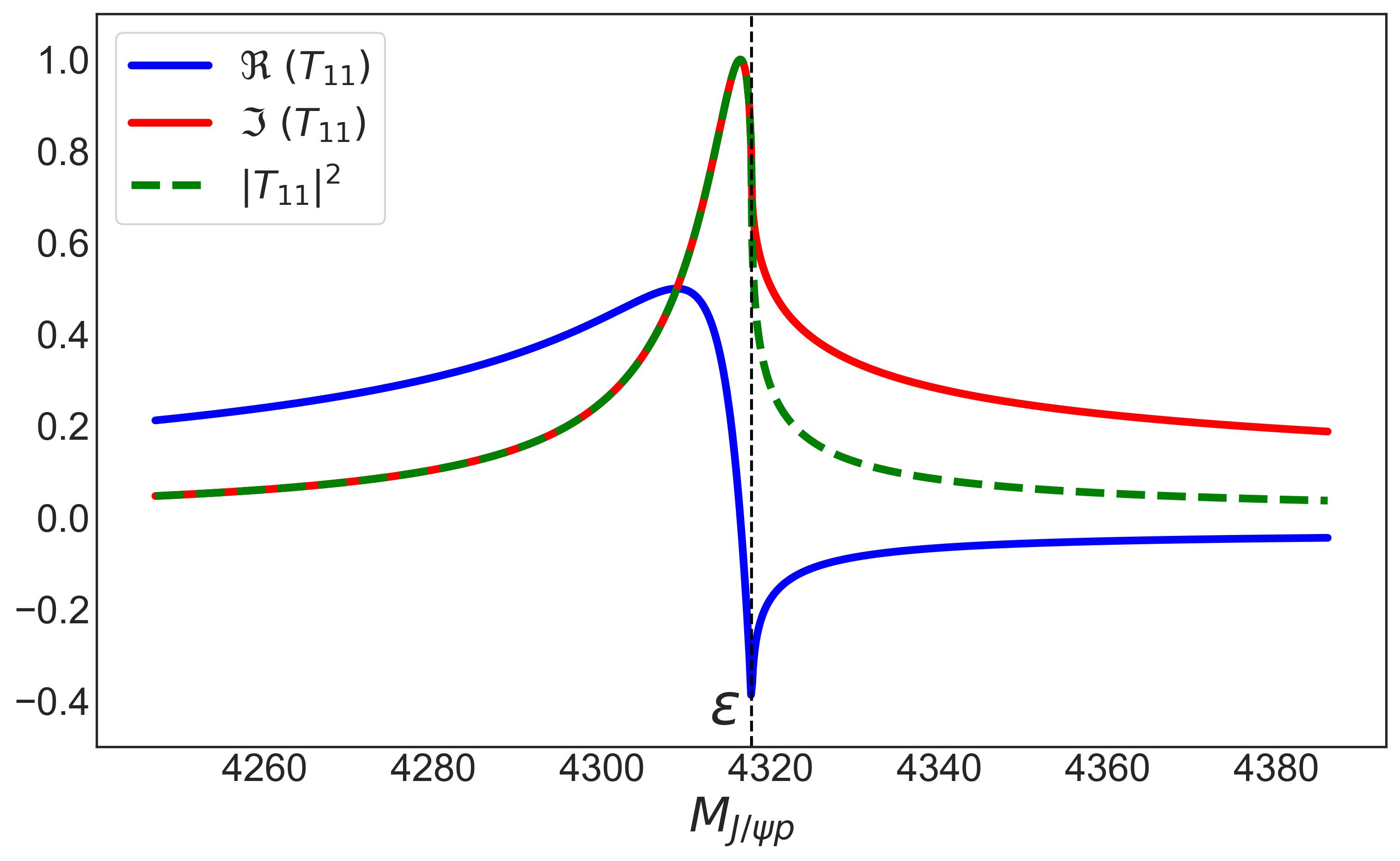
(a)

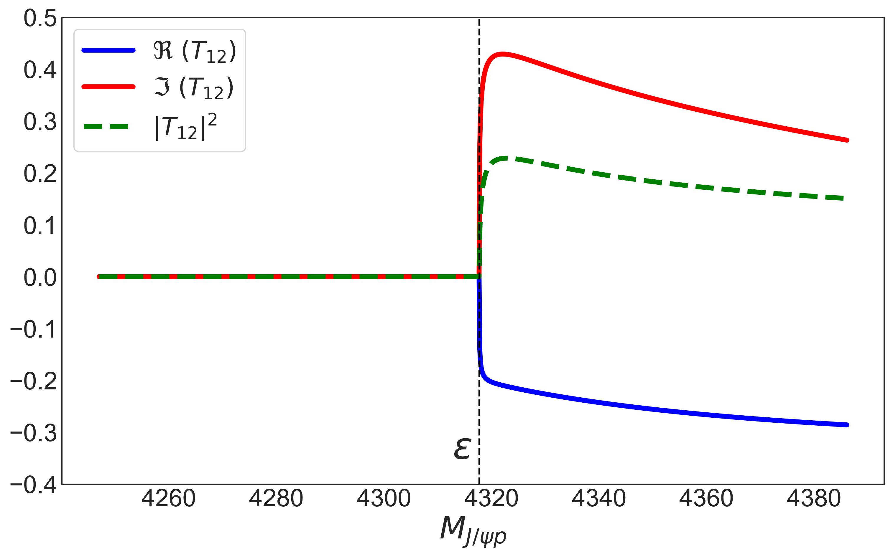
(b)

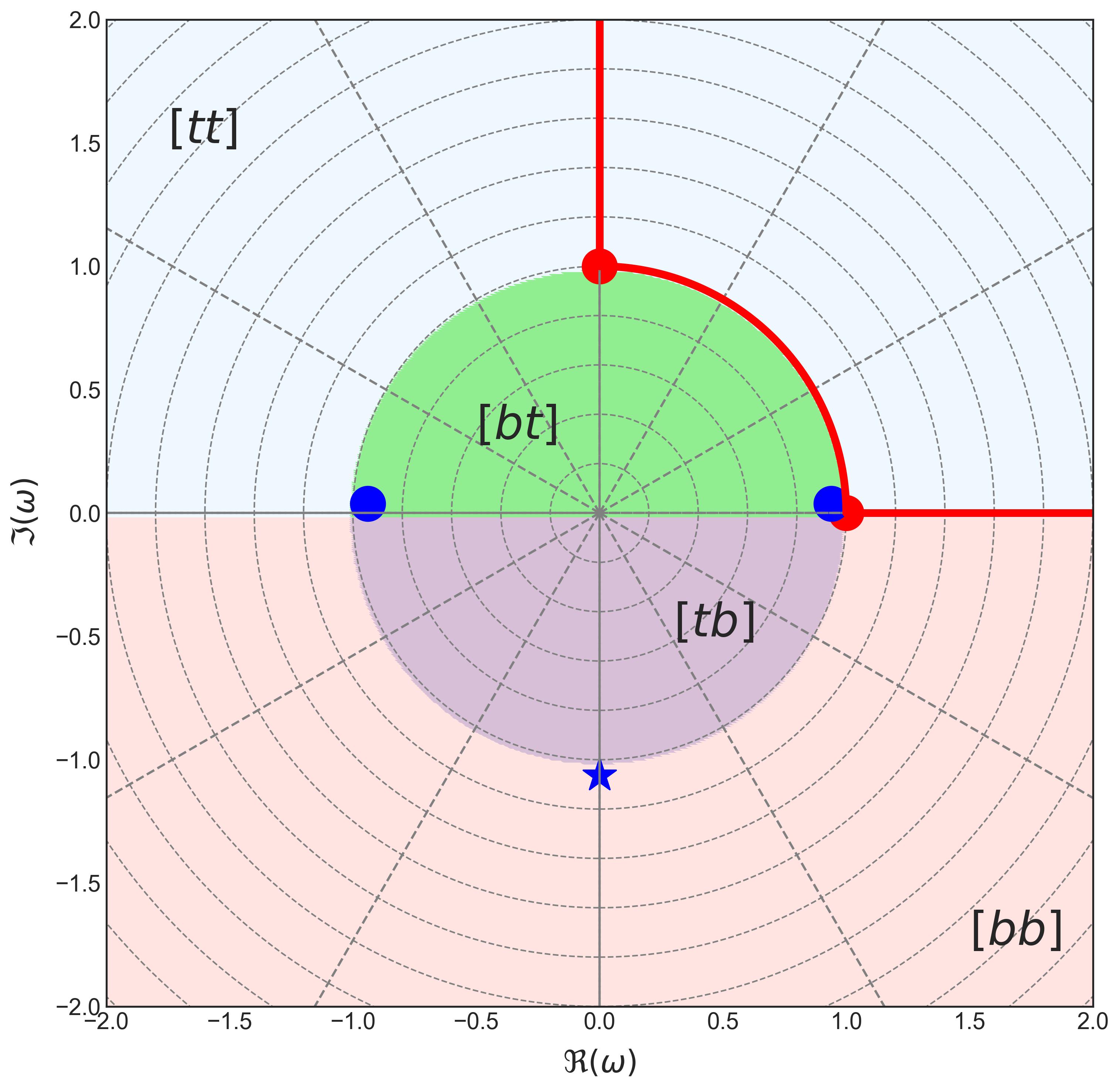
(c)

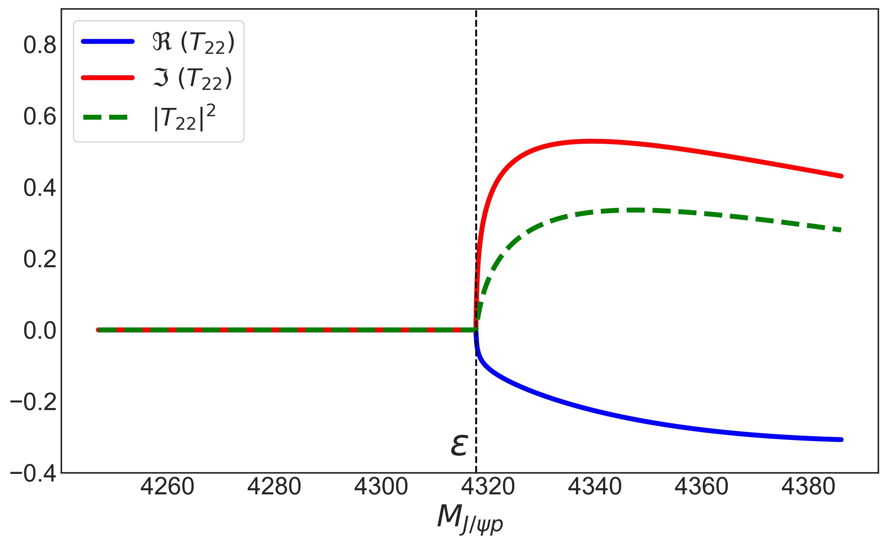
(d)

Figure 2: Elements of the $T$-matrix with a pole on the $[bt]$ sheet, signifying a molecular nature based on pole counting method.

By looking only at the $T_{11}$ matrix element, its sharp peak near the $\Sigma_{c}\bar{D}$ threshold hints a signature of a molecular state. We can back this up by appealing to the pole counting method which, for an isolated pole in $[bt]$ sheet, suggests a molecular nature of the observed signal. On the other hand, both the bottom-top approach done in Fernández-Ramírez et al. (2019) and Ng et al. (2022) which utilized the form

$$\frac{\mathrm{d}N}{\mathrm{d}\sqrt{s}}=\rho(s)\left[|P(s)T(s)|^{2}+B(s)\right]$$ (15)

where $P(s)$ and $B(s)$ are smooth functions, $\rho(s)$ the three-body phase space and $T(s)$ being the $T_{11}$ matrix element had concluded that the signal is likely due to a virtual state. As mentioned earlier, near-threshold virtual states are molecular in nature as long as range corrections can be neglected Matuschek et al. (2021), and hence the agreement with the pole couting method and the conclusions in Fernández-Ramírez et al. (2019) and Ng et al. (2022). However, it is noteworthy to mention that the recent investigation of the same signal using deep learning in Zhang et al. (2023) favors the compact interpretation.

We move on to the next configuration. We use the same isolated pole in $[bt]$ sheet from the previous configuration plus an additional ambiguous pair poles on the $[bb]$ and $[tb]$ sheets. The values of the added poles are set to produce an ambiguous pair of poles as described in the previous subsection. Specifically, we set the pair poles such that their real parts are $4317.73$ MeV and $12.5$ MeV for its widths. The three-pole configuration and its $T$-matrix elements are shown in Fig. 3.

(a)

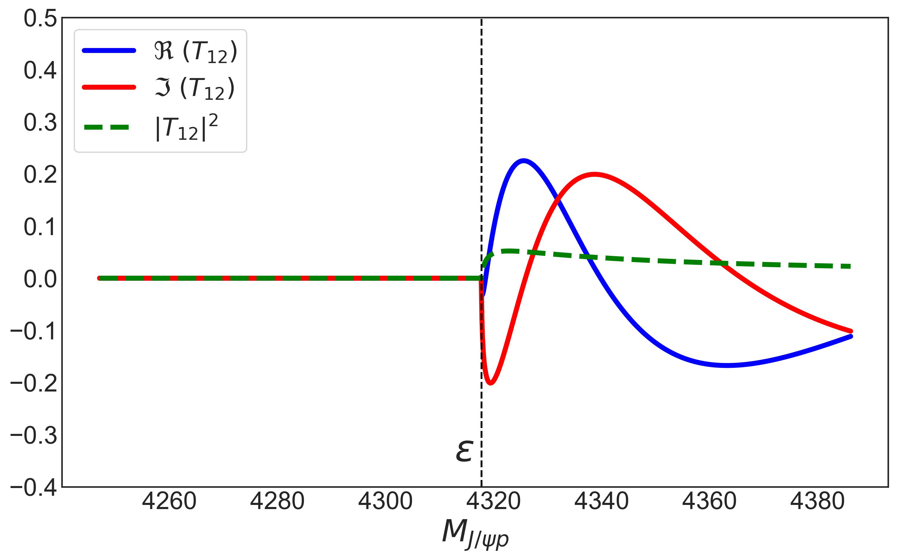
(b)

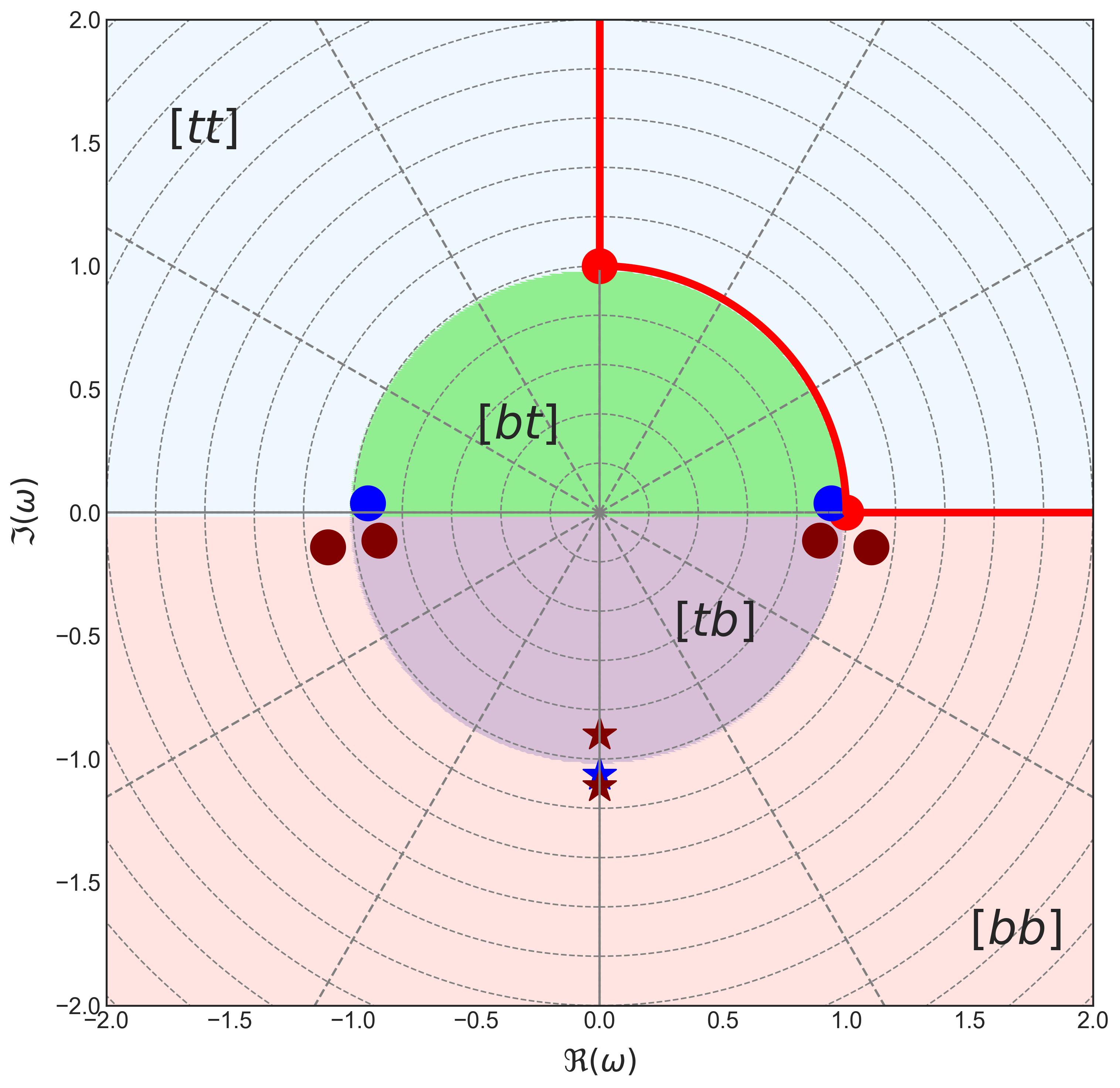
(c)

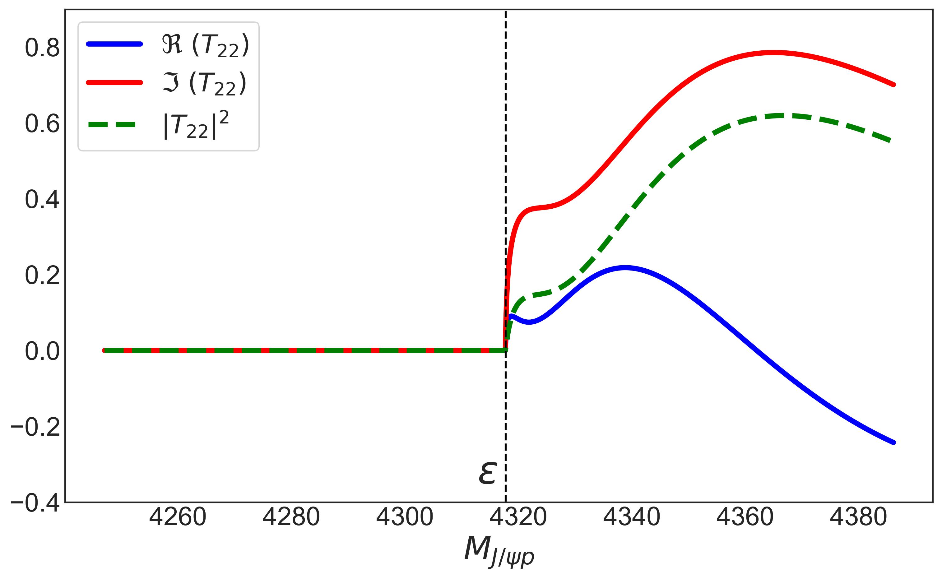
(d)

Figure 3: Elements of the $T$-matrix with an isolated pole on the $[bt]$, $[bb]$, and $[tb]$ sheets. Can be interpreted having a non-molecular nature based on pole counting method.

The interpretation of 3-pole configuration is now outside the direct applicability of the pole counting argument. We are confronted with different possible scenarios for the occurrences of such pole structures. One naive interpretation is that the $[bt]$ sheet pole is a molecular state of the $\Sigma_{c}\bar{D}$ channel with the added $[bb]$ and $[tb]$ poles as some non-molecular state that is strongly coupled to $\Sigma_{c}\bar{D}$ channel. However, such interpretation is unlikely since the real parts of the $[bb]$ and $[tb]$ poles are exactly placed at the second threshold. This means that there is no available phase space for the unstable state to decay into the second channel.

A more plausible interpretation is that the $[tb]$ sheet pole is a virtual state of the $\Sigma_{c}\bar{D}$ channel and the remaining $[bt]$ and $[bb]$ poles correspond to a compact state that is strongly coupled to the $J/\psi p$ channel. Unlike the first interpretation, there is enough phase space for such a compact resonance to decay into $J/\psi p$ channel. Interestingly, this scenario matches the hybrid model proposed in Yamaguchi et al. (2017, 2020). Comparing the $T_{11}$ line shape in Fig. 2, which admits a purely molecular interpretation, and $T_{11}$ in Fig. 3, one can interpret that a compact state combined with a virtual state can lead to a purely molecular-like interpretation. That is, the compact state enhances the attraction of the hadrons in the higher mass channel.

Certainly, there is an obvious ambiguity in the interpretation of $T_{11}$ line shape with the 1-pole and the 3-pole structures. Their distinction will only become evident when we probe either the off-diagonal $T_{21}$ element or the elastic $T_{22}$ amplitude. Considering that the available data came from the decay $\Lambda_{b}\rightarrow K^{-}J/\psi p$, it is appropriate to include the contribution of $T_{21}$ transition when computing for the invariant mass distribution of $J/\psi p$ to determine the presence of ambiguous pair of poles.

III.3 On the necessity of probing the $T_{12}$ amplitude

The condition for the existence of ambiguous pair poles, i.e. poles in different Riemann sheets but with exactly the same position, is highly fine tuned. More realistic situation may have poles in different Riemann sheets but not necessarily with the same position due to possible contamination of coupled channel effects. That is, there maybe a slight difference in the line shape of $T_{11}$ for different pole structures. However, when the error bars of the experimental data are large then any distinction among the $T_{11}$s with different pole structures will no longer be useful. The inclusion of $|T_{21}|^{2}$ might help since the 1-pole structure has slightly larger $|T_{21}|^{2}$ in comparison with the 3-pole structure.

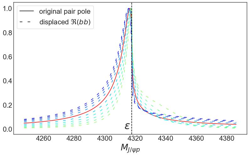
(a)

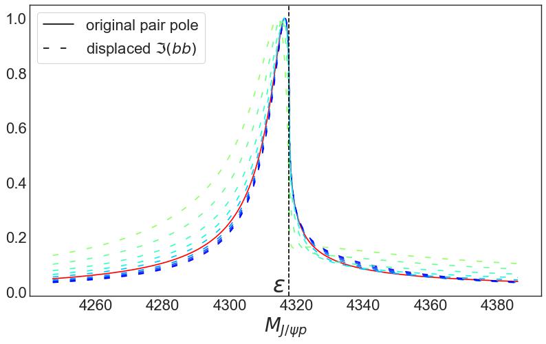
(b)

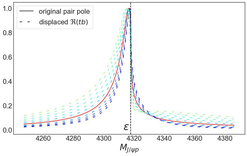
(c)

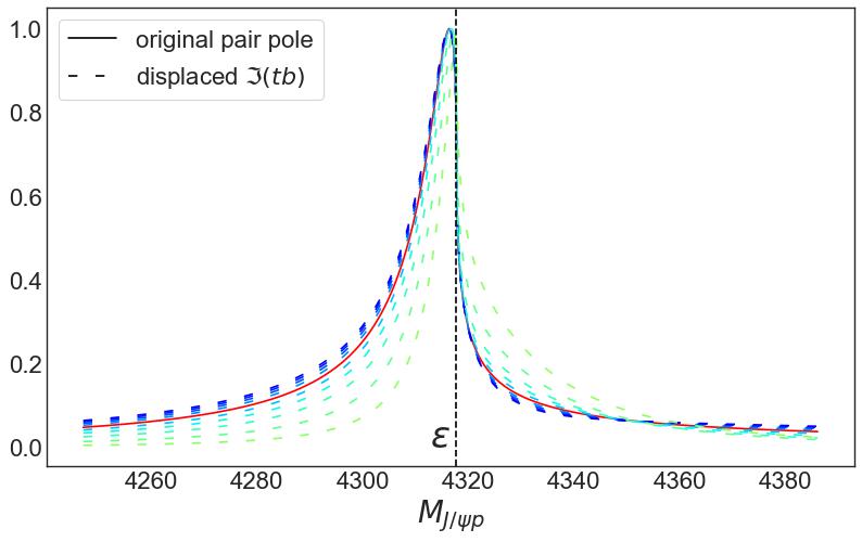
(d)

Figure 4: Displacing one of the pair poles and fixing the other. The darker color hues represent the displacement below the original $\real$ ($\imaginary$) and the lighter hues represent the displacement above the original $\real$ ($\imaginary$) values. Quantitatively, there is little to no difference near the threshold.

To further demonstrate the importance of $|T_{21}|^{2}$, we consider the $P^{N}_{\psi}(4312)^{+}$ in the invariant mass spectrum of $J/\psi p$. We construct an $S$-matrix similar to that of the 3-pole configuration example above. Afterwards, we displace either the real or the imaginary part of one of the pair poles while fixing in place the other. In this way, the ambiguous pair poles are less fine tuned. The respective $T_{11}$ amplitude line shapes are then plotted in figure 4. Notice that the tail of line shape is sensitive to the presence of ambiguous poles. However, the peak structure for all cases are almost similar despite their differences in their tail. This might entail a problem if the error bars obscured the distinction of ambiguous line shapes near the threshold. It is also possible that the line shape of the slightly displaced ambiguous pair poles might be absorbed by the background parametrizations if the amplitude ansatz is limited to produce one isolated pole near the threshold. It was shown in Frazer and Hendry (1964) that the effective range expansion cannot produce a pole on the $[bb]$ sheet due to the impossibility of making the real and imaginary parts of the amplitude’s denominator simultaneously equal to zero. Such restriction limits the model space of a given line shape to molecular-like bound or virtual states and immediately rules out compact state interpretation.

IV Conclusion and outlook

The method of independent S-matrix poles is a useful tool in analyzing near-threshold phenomena in a model-independent way. We have shown that in our formulation, it is possible that some of the commonly used analyses missed out important physics in probing the nature of near-threshold enhancements. The parametrized background may absorb the relevant physics if the parametrization used can only cover a limited model space. Other elements of the full S-matrix can be useful in providing a more rigorous interpretations of the observed signals.

We used the independent S-matrix poles formulation to study the $P_{\psi}^{N}(4312)^{+}$ in the invariant mass spectrum of $J/\psi p$. It turned out that, by focusing only on the contribution of $T_{11}$ in the overall line shape of the distribution, one cannot rule out yet the compact pentaquark interpretation. Our result gives credence to the deep learning analysis made in Zhang et al. (2023) and the improved data in Adhikari et al. (2023) together with its corresponding analysis in Strakovsky et al. (2023). It is also worth noting that a three-channel analysis upholding the principles of S-matrix in Winney et al. (2023) shows evidence of poles near the scattering region, emphasizing the importance of strong coupling with higher channels. Indeed, sophisticated methods catering all possibilities must be considered to obtain a definitive interpretation of the pentaquark signals.

Moving forward, we plan to use the present formalism to improve the deep learning extraction of pole configurations started in Sombillo et al. (2020, 2021b, 2021a). The independence of the poles used in generating the line shape ensures that no specific trajectory is preferred to reach a particular pole configuration. Together with the vast parameters that a deep neural network can provide and its ability to generalize beyond the training dataset, one can then extract a non-biased interpretation of near-threshold enhancements.

References

- Olsen et al. (2018) S. L. Olsen, T. Skwarnicki, and D. Zieminska, Rev. Mod. Phys. 90, 015003 (2018), arXiv:1708.04012 [hep-ph] .
- Guo et al. (2018) F.-K. Guo, C. Hanhart, U.-G. Meißner, Q. Wang, Q. Zhao, and B.-S. Zou, Rev. Mod. Phys. 90, 015004 (2018), arXiv:1705.00141 [hep-ph] .
- Oller (2020) J. A. Oller, Prog. Part. Nucl. Phys. 110, 103728 (2020), arXiv:1909.00370 [hep-ph] .
- Guo et al. (2020) F.-K. Guo, X.-H. Liu, and S. Sakai, Prog. Part. Nucl. Phys. 112, 103757 (2020), arXiv:1912.07030 [hep-ph] .
- Mai et al. (2023) M. Mai, U.-G. Meißner, and C. Urbach, Phys. Rept. 1001, 1 (2023), arXiv:2206.01477 [hep-ph] .
- Albaladejo et al. (2022) M. Albaladejo et al., Progress in Particle and Nuclear Physics 127, 103981 (2022).
- Aaij et al. (2019) R. Aaij et al. (LHCb Collaboration), Phys. Rev. Lett. 122, 222001 (2019).
- Aaij et al. (2015) R. Aaij et al. (LHCb Collaboration), Phys. Rev. Lett. 115, 072001 (2015).
- Fernández-Ramírez et al. (2019) C. Fernández-Ramírez, A. Pilloni, M. Albaladejo, A. Jackura, V. Mathieu, M. Mikhasenko, J. A. Silva-Castro, and A. P. Szczepaniak (JPAC), Phys. Rev. Lett. 123, 092001 (2019), arXiv:1904.10021 [hep-ph] .
- Ng et al. (2022) L. Ng, L. Bibrzycki, J. Nys, C. Fernández-Ramírez, A. Pilloni, V. Mathieu, A. J. Rasmusson, and A. P. Szczepaniak (Joint Physics Analysis Center), Phys. Rev. D 105, L091501 (2022).
- Chen et al. (2019) H.-X. Chen, W. Chen, and S.-L. Zhu, Phys. Rev. D 100, 051501 (2019).
- Cheng and Liu (2019) J.-B. Cheng and Y.-R. Liu, Phys. Rev. D 100, 054002 (2019).
- Du et al. (2020) M.-L. Du, V. Baru, F.-K. Guo, C. Hanhart, U.-G. Meißner, J. A. Oller, and Q. Wang, Phys. Rev. Lett. 124, 072001 (2020).
- Matuschek et al. (2021) I. Matuschek, V. Baru, F.-K. Guo, and C. Hanhart, The European Physical Journal A 57, 101 (2021).
- Ali and Parkhomenko (2019) A. Ali and A. Y. Parkhomenko, Physics Letters B 793, 365 (2019).
- Morgan (1992) D. Morgan, Nucl. Phys. A 543, 632 (1992).
- Morgan and Pennington (1991) D. Morgan and M. Pennington, Phys. Lett. B 258, 444 (1991).
- Morgan and Pennington (1993) D. Morgan and M. R. Pennington, Phys. Rev. D 48, 5422 (1993).
- Newton (1982) R. G. Newton, Scattering Theory of Waves and Particles, Theoretical and Mathematical Physics (Springer-Verlag Berlin Heidelberg, 1982).
- Kato (1965) M. Kato, Annals of Physics 31, 130 (1965).
- Yamada and Morimatsu (2020) W. Yamada and O. Morimatsu, Phys. Rev. C 102, 055201 (2020).
- Yamada and Morimatsu (2021) W. A. Yamada and O. Morimatsu, Phys. Rev. C 103, 045201 (2021).
- Yamada et al. (2022) W. A. Yamada, O. Morimatsu, T. Sato, and K. Yazaki, Phys. Rev. D 105, 014034 (2022).
- Taylor (1972) J. Taylor, Scattering Theory: Quantum Theory on Nonrelativistic Collisions (Wiley, 1972).
- van Kampen (1953a) N. G. van Kampen, Phys. Rev. 91, 1267 (1953a).
- van Kampen (1953b) N. G. van Kampen, Phys. Rev. 89, 1072 (1953b).
- Rakityansky (2022) S. A. Rakityansky, “Riemann surfaces for multi-channel systems,” in Jost Functions in Quantum Mechanics: A Unified Approach to Scattering, Bound, and Resonant State Problems (Springer International Publishing, Cham, 2022) pp. 407–423.
- Pearce and Gibson (1989) B. C. Pearce and B. F. Gibson, Phys. Rev. C 40, 902 (1989).
- Frazer and Hendry (1964) W. R. Frazer and A. W. Hendry, Phys. Rev. 134, B1307 (1964).
- Couteur (1960) K. J. L. Couteur, Proc. R. Soc. Lon. A. 256, 115 (1960).
- Newton (1961) R. G. Newton, J. Math. Phys. 2, 188 (1961).
- Newton (1962) R. G. Newton, J. Math. Phys. 3, 75 (1962).
- Badalyan et al. (1982) A. M. Badalyan, L. P. Kok, M. I. Polikarpov, and Y. A. Simonov, Phys. Rep. 82, 31 (1982).
- Hanhart et al. (2014) C. Hanhart, J. R. Pelaez, and G. Rios, Phys. Lett. B 739, 375 (2014), arXiv:1407.7452 [hep-ph] .
- Hyodo (2014) T. Hyodo, Phys. Rev. C 90, 055208 (2014), arXiv:1407.2372 [hep-ph] .
- Workman et al. (2022) R. L. Workman et al. (Particle Data Group), PTEP 2022, 083C01 (2022).
- Wang et al. (2021) Z.-Y. Wang, H. A. Ahmed, and C. W. Xiao, Eur. Phys. J. C 81, 833 (2021), arXiv:2106.10511 [hep-ph] .
- Meißner (2020) U.-G. Meißner, Symmetry 12, 981 (2020), arXiv:2005.06909 [hep-ph] .
- Hyodo and Jido (2012) T. Hyodo and D. Jido, Prog. Part. Nucl. Phys. 67, 55 (2012), arXiv:1104.4474 [nucl-th] .
- Kuang et al. (2020) S.-Q. Kuang, X.-W. Dai, Ling-Yun andKang, and D.-L. Yao, The European Physical Journal C 80, 11 (2020).
- Sombillo et al. (2021a) D. L. B. Sombillo, Y. Ikeda, T. Sato, and A. Hosaka, Phys. Rev. D 104, 036001 (2021a).
- Eden and Taylor (1964) R. J. Eden and J. R. Taylor, Phys. Rev. 133, B1575 (1964).
- Zhang et al. (2023) Z. Zhang, J. Liu, J. Hu, Q. Wang, and U.-G. Meißner, Science Bulletin 68, 981 (2023).
- Yamaguchi et al. (2017) Y. Yamaguchi, A. Giachino, A. Hosaka, E. Santopinto, S. Takeuchi, and M. Takizawa, Phys. Rev. D 96, 114031 (2017), arXiv:1709.00819 [hep-ph] .
- Yamaguchi et al. (2020) Y. Yamaguchi, A. Hosaka, S. Takeuchi, and M. Takizawa, J. Phys. G 47, 053001 (2020), arXiv:1908.08790 [hep-ph] .
- Adhikari et al. (2023) S. Adhikari et al. (GlueX), Phys. Rev. C 108, 025201 (2023), arXiv:2304.03845 [nucl-ex] .
- Strakovsky et al. (2023) I. Strakovsky, W. J. Briscoe, E. Chudakov, I. Larin, L. Pentchev, A. Schmidt, and R. L. Workman, Phys. Rev. C 108, 015202 (2023), arXiv:2304.04924 [hep-ph] .
- Winney et al. (2023) D. Winney et al., (2023), arXiv:2305.01449 [hep-ph] .
- Sombillo et al. (2020) D. L. B. Sombillo, Y. Ikeda, T. Sato, and A. Hosaka, Phys. Rev. D 102, 016024 (2020).
- Sombillo et al. (2021b) D. L. B. Sombillo, Y. Ikeda, T. Sato, and A. Hosaka, Few-Body Systems 62, 52 (2021b).