Symmetry-Preserving Program Representations for Learning Code Semantics

Abstract

Large Language Models (LLMs) have shown promise in automated program reasoning, a crucial aspect of many security tasks. However, existing LLM architectures for code are often borrowed from other domains like natural language processing, raising concerns about their generalization and robustness to unseen code. A key generalization challenge is to incorporate the knowledge of code semantics, including control and data flow, into the LLM architectures.

Drawing inspiration from examples of convolution layers exploiting translation symmetry, we explore how code symmetries can enhance LLM architectures for program analysis and modeling. We present a rigorous group-theoretic framework that formally defines code symmetries as semantics-preserving transformations and provides techniques for precisely reasoning about symmetry preservation within LLM architectures. Using this framework, we introduce a novel variant of self-attention that preserves program symmetries, demonstrating its effectiveness in generalization and robustness through detailed experimental evaluations across different binary and source code analysis tasks. Overall, our code symmetry framework offers rigorous and powerful reasoning techniques that can guide the future development of specialized LLMs for code and advance LLM-guided program reasoning tasks.

1 Introduction

Automated program analysis is vital for security tasks such as vulnerability investigation [69, 74, 68, 39], malware analysis [23, 55, 83], and reverse engineering [70, 72]. Deep learning, especially with large language models (LLMs), has shown promise in various code modeling tasks for security applications [46, 80, 79, 49, 58, 47, 76, 36, 9, 38, 13]. However, generalizability and robustness to unseen code continue to raise significant concerns [34, 65, 28, 82, 12, 84].

Current LLM architectures for code are often borrowed from other domains like vision and natural language processing. The challenge is to incorporate the knowledge of program semantics, including control/data flow, into LLM architectures by design without explicit enumeration in training samples. In this paper, we address this challenge by establishing foundational symmetries for code. Inspired by translation symmetry in vision, which led to the design of convolution layers, we explore how incorporating similar symmetry-preserving considerations (e.g., permutation symmetry) can improve code analysis and modeling.

Code symmetry. Intuitively, symmetry of code refers to any transformation applied to a code block that preserves the semantics (i.e., input-output behavior) of the original code (see §4.2 for a more formal definition). For example, these transformations may include operations such as code reordering, variable renaming, or loop unrolling. Consider a (sequential) code fragment x=2;y=4. Reordering the instructions to y=4;x=2 does not change the semantics (i.e., the input-output behavior). Of course, any code analysis task that depends solely on the semantics of the code (e.g., vulnerability discovery and malware analysis) needs to preserve these symmetries by remaining invariant to the transformations, i.e., an ideal, generalized LLM $m$ should have the same output for all semantics-preserving variants. Formally, given a code block $c$ and a set of symmetries $G$, $\forall g\in G,m(g(c))=m(c)$.

Limitations of existing approaches. A popular way to indirectly teach an LLM to preserve the symmetries of code is data augmentation and pre-training [47, 76, 20, 9]. This involves applying different semantics-preserving transformations from the set $G$ to an existing code block $c$, thereby generating a large number of additional training/pre-training examples. However, this approach has two major limitations. First, it is often prohibitively expensive to exhaustively train an LLM on all augmented samples generated from even a single code block and a given transformation. For instance, the number of ways to reorder instructions within a code block while still preserving its input-output behavior can grow factorially with the number of instructions in the code block [71]. Second, even if the model can be trained on all these enumerations, there is no guarantee that the model will learn to be invariant to these transformations in $G$.

Our approach. We propose a group-theoretic approach that provides the theoretical foundation to design new LLM architectures guaranteed to preserve code symmetries by construction and achieve the desired invariance as long as the set of symmetries forms a group. Informally, a group of symmetries is a set of symmetries that has an additional composition operation allowing any two symmetries to be composed into potentially new symmetries while following certain algebraic axioms (see §3 for a formal definition). We define a code symmetry group as a group of symmetries that preserve code semantics. For example, all permutations (i.e., reorderings) of the instructions of a code block that preserve code semantics form a code symmetry group.

Our key insight behind using a group structure is that a symmetry group has a (often small) set of generators and a composition operation from which all symmetries in the group can be generated. Therefore, for an LLM, as long as we can prove that the desired invariant properties hold for all of the generator transformations and the composition operation, we automatically guarantee the invariants to hold for all possible transformations in the entire group without having to individually reason about different possible compositions. We further introduce a mechanism for identifying a semantics-preserving group of permutation symmetries of a code block based on detecting graph automorphisms of the interpretation graph (see §4.3 for a formal definition) of the code block.

In this paper, we present SymC, a new LLM architecture for code based on a novel variant of self-attention that can provably preserve a given semantics-preserving code symmetry group and achieve the desired invariance. Our model, by construction, is guaranteed to be robust to semantics-preserving instruction/statement permutations. Empirically, our approach generalizes effectively to many other types of program transformations beyond permutations (§6.4).

To understand how we enforce the desired invariance in SymC, we need to understand some details about the internal computations of the model. LLMs primarily consist of two high-level components: representation learning and predictive learning [17, 35]. As part of representation learning, the early layers of LLMs aim to encode input programs (either in source or binary form) into a high-dimensional real vector space, preserving relevant program features, patterns, and relationships. Formally, a representation function $r$ maps code block $c$ containing $n$ instructions/statements from instruction set $I$ to a point in a $d$-dimensional real vector space $\mathbb{R}^{d\times n}$, $r:I^{n}\rightarrow\mathbb{R}^{d\times n}$. Subsequently, these learned representations or embeddings are used for the downstream predictive tasks. Formally, the predictive task is represented by a function $p:\mathbb{R}^{d\times n}\rightarrow\mathbb{R}^{L}$ where ${R}^{L}$ is the label-space specific to the task. Therefore, the entire LLM can be thought of as a composition of $p$ and $r$, i.e., $p\circ r$.

Equivariance of representations. We achieve the desired invariance property of an LLM’s output wrt. a given semantics-preserving code symmetry group in two steps: (1) enforcing that the learned representations preserve the symmetry group structure in a certain way called equivariance (formally defined in §4.1). Intuitively, equivariance means the results of applying any transformation from the symmetry group on the representation of a code block is the same as applying the transformation first on the code block and then learning the representation of the transformed code. Formally, $\forall c$ in training data, $\forall g\in G,r(g(c))=g(r(c))$. (2) making the prediction function to be invariant. We prove that their composition is guaranteed to achieve the desired invariance properties, i.e., $\forall c$ in training data, $\forall g\in G,p\circ r(g(c))=p\circ r(c)$.

An astute reader might at this point wonder, why we are not enforcing invariance on the representations themselves, i.e., ensuring all the semantically-equivalent code blocks be mapped to the same point in the real vector space. As LLMs are expected to generalize both in terms of code blocks and unseen transformations based on the training samples and their symmetry groups, such invariant representations are not very useful as they discard all information about the applied transformations. By contrast, equivariant representation learning is better suited for generalization by preserving the structure of semantics-preserving transformations and their influence on the input [35, 52]. We empirically demonstrate this effect in §7.3 that the earlier invariant layers in the representation learning, the worse the performance we obtain (e.g., dropped by 60.7%).

Result summary. We extensively evaluate SymC on four program analysis tasks, covering both source code and binary. These tasks involve predicting function name and signature, detecting function similarity, and memory region prediction. We compare SymC against various semantics-preserving program transformations, including those introduced by different compilers, optimizations, obfuscations, and source-level program rewriting. The results show that SymC outperforms the state-of-the-art baselines, even those requiring significant pre-training effort, by an average of 36.8%. Furthermore, in resource-constrained settings, SymC reaches the comparable performance to pre-trained baselines while estimated to cost 1,281$\times$ less power and emitted carbon dioxide, making it an efficient and eco-friendly solution.

Overall, this paper makes the following contributions:

• We establish a foundational framework based on semantics-preserving code symmetry groups, allowing for provable generalization to new samples generated by compositions of symmetries.

• We provide formal definitions and theoretical insights essential for effective reasoning of semantics-preserving symmetries in programs.

• We introduce a mechanism for identifying a group of symmetries for a given program using graph automorphism of the interpretation graph of the program.

• We present a novel LLM architecture incorporating a new type of self-attention mechanism that is equivariant to a program’s symmetry groups.

• Through extensive experimental evaluation on a diverse set of source and binary analysis tasks, we demonstrate the effectiveness of our approach in terms of both generalization and robustness.

2 Motivating Example

(a) $G$-invariant code analysis

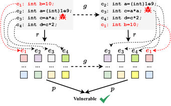
(b) $G$-invariant vulnerability detector

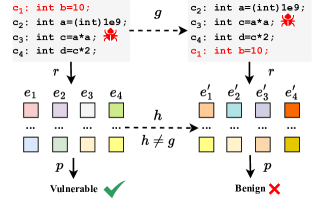
(c) Symmetry-breaking vulnerability detector

Figure 1: (a) High-level summary of $G$-equivariant code representation learning (Definition 4.4) and $G$-invariant predictive learning (Definition 4.5). (b) An $G$-invariant, i.e., the representation does not change (in color), vulnerability detector, e.g., based on matching semantically similar vulnerable code (see §6.1 for task description) where $G$ is a group of semantics-preserving statement permutations $g$. (c) A vulnerability predictor, e.g., regular Transformer, that does not preserve the symmetries in $G$, i.e., the learned representation of each statement completely changes when the statements are permuted (in color), and thus incorrectly predicts a vulnerable code as benign even when the transformed code is semantically equivalent to the original.

Before formally defining semantics-preserving symmetries and their significance in generalizability, we present an intuitive example to illustrate our symmetry-preserving construction. Figure 1a depicts the conceptual design of the representation learning $r:I^{n}\rightarrow\mathbb{R}^{d\times n}$ and predictive learning $p:\mathbb{R}^{d\times n}\rightarrow\mathbb{R}^{L}$ components in LLMs. (§4.1 includes the formal definitions of $p$ and $r$.) We design representation learning $r$ to be equivariant and predictive learning $p$ to be invariant to the symmetry group.

Figure 1b demonstrates a vulnerability predictor ($p\circ r$) satisfying $G$-invariance with respect to a permutation group $G$. The code snippets with an integer overflow vulnerability illustrate a semantics-preserving statement reordering. Such permutations should not change the final prediction (i.e., vulnerable), as $c_{1}$ has no data/control dependency with the other lines. This intuition is enforced through $G$-invariance, ensuring the final vulnerability prediction remains unchanged (i.e., vulnerable), and $G$-equivariance, where the code representation $(e_{1},...,e_{4})$ is transformed into $(e_{2},...,e_{4},e_{1})$, preserving equivariance to the permutations in $G$.

By contrast, Figure 1c provides an example where a vulnerability predictor has a representation $r$ that does not preserve permutation symmetry of reordering $c_{1}$ (i.e., a regular transformer model). In this case, the code representation $(e_{1},...,e_{4})$ is transformed into a different set of vectors $(e^{\prime}_{1},...,e^{\prime}_{4})$. Consequently, this inaccurate representation leads to incorrectly predicting the code snippet to be benign.

3 Preliminaries

This section formally defines the symmetry group and the invariance and equivariance properties against the symmetry group. The later description of our symmetry-preserving code analysis models (§4) builds on these concepts.

Symmetry group. Intuitively, a symmetry is a transformation or operation on an object that preserves certain properties of the object. For example, in the context of image classification, a rotation operation acting on an image of a ball, which does not change the label of the ball, can be considered a symmetry. A symmetry group is a set of such symmetries with some additional properties. An arbitrary set of symmetries does not always form a symmetry group. To form a symmetry group, a set of operations must possess certain additional properties as described below.

Definition 3.1.

A symmetry group $(G,\circ)$ consists of a non-empty set $G$ of transformations and a binary operator $\circ:G\times G\rightarrow G$, where $\circ$ operates on two elements (i.e., transformations) in $G$, e.g., $x,y\in G$, and produces a new transformation $z=x\circ y$. $(G,\circ)$ should satisfy four axioms:

• Associativity: $\forall x,y,z\in G,x\circ(y\circ z)=(x\circ y)\circ z$

• Identity: $\exists\mathbf{1}\in G,\forall x\in G,x\circ\mathbf{1}=\mathbf{1}\circ x$

• Inverse: $\forall x\in G,\exists x^{-1}\in G,x\circ x^{-1}=\mathbf{1}$

• Closure: $\forall x,y\in G,x\circ y\in G$

Action of a symmetry group. As defined above, the elements of a $G$ are abstract transformations that become concrete when they act on some set $X$, i.e., they transform some object $x\in X$ into another object $x^{\prime}\in X$ while keeping some properties of the object invariant. Formally, an action of a symmetry group $G$ is defined as follows:

Definition 3.2.

An action $\bullet$ of a symmetry group $(G,\circ)$ is a binary operation defined on a set of objects $X$, i.e., $\bullet:G\times X\rightarrow X$, where

• Identitiy: $\forall x\in X,\mathbf{1}\bullet x=x$

• Compatibility: $\forall g,h\in G,x\in X,(g\circ h)\bullet x=g\bullet(h\bullet x)$

As a concrete example, $X$ can be a set of programs and $G$ can be all possible instruction permutations that preserve the input-output behavior of the programs in $X$. It might seem unclear at this point how these permutations form a group (satisfying group axioms). We will formalize the notion of permutations and their actions on programs in §4.3.

Notation. It is common in the group theory literature to use $\circ$ to denote both action and composition, when it is clear from the context which operation is being used [35]. For example, $(g\circ h)\circ x$ denotes composing the two transformations $g$ and $h$ and then letting the composite transformation act on an object $x$. It is also customary to interchange $g(x)$ and $g\circ x$ where both denote applying a function/action on $x$. Therefore, we treat $g\bullet(h\bullet x)$, $g\circ(h\circ x)$, and $g(h(x))$ as the same and follow this convention in the rest of this paper.

Invariance and equivariance. A symmetry group comes with two properties, namely invariance and equivariance, that formalize the concept of preservation of some properties when a set $X$ is acted upon by the symmetry group $G$. Invariance refers to the property that remains unchanged under the action of the symmetry group. Equivariance, on the other hand, expresses the compatibility between the action of the symmetry group and the property.

To define this more precisely, we need to introduce a function $f:X\rightarrow Y$, where $X$ is the set under consideration and $Y$ is the co-domain representing the range of possible values associated with the property of interest. The function $f$ maps each element $x\in X$ to a corresponding element $y$ in the set $Y$, indicating the property’s value for that particular element. We now define the equivariance and invariance of $f$ operating on $X$ against the group operations in $G$.

Definition 3.3.

Let $f:X\rightarrow Y$ be a function where $X$ and $Y$ are two sets and $G$ be the symmetry group that acts on both sets $X$ and $Y$.

• Invariant: $f$ is called $G$-invariant if $\forall g\in G,\forall x\in X,f(g\circ x)=f(x)$.

• Equivariant: $f$ is called $G$-equivariant if $\forall g\in G,\forall x\in X,f(g\circ x)=g\circ f(x)$.

Given the definition of $G$-equivariant function, we have the following lemmas (we leave their proofs in Appendix B as they are straightforward):

Lemma 1 (The composition of two $G$-equivariant functions is also $G$-equivariant).

Let $f_{1}$ and $f_{2}$ be two functions that are both $G$-equivariant and $h=f_{1}\circ f_{2}$ be the new function composed by $f_{1}$ and $f_{2}$. $h$ is also $G$-equivariant.

Lemma 2 (The composition of a $G$-equivariant function and $G$-invariant function is $G$-invariant).

Let $f_{1}$ and $f_{2}$ be two functions where $f_{1}$ is $G$-equivariant $f_{2}$ is $G$-invariant, and $h=f_{2}\circ f_{1}$ be the new function composed by applying $f_{1}$ and then $f_{2}$. $h$ is $G$-invariant.

We will use Lemma 1 and Lemma 2 extensively in §4 to show how SymC, composed by multiple neural modules including $G$-equivariant embedding layers, $G$-equivariant self-attention layers, and $G$-invariant prediction heads lead to $G$-invariant code analysis models.

4 Methodology

In this section, we start from describing the significance of staying invariant and equivariant to symmetries (input transformations) in the context of code models. We then formalize the desired properties of these program symmetries as being semantics-preserving. We then describe a subset of the program symmetries that forms a program symmetry group, based on the automorphism group of a program interpretation graph, and how we can leverage the group structure to guide the development of group-equivariant self-attention layers. Finally, we describe typical group-invariant predictors so that stacking them on top of group-equivariant self-attention layers leads us to a group-invariant code analysis model (Lemma 2).

4.1 Invariance & Equivariance for Code Models

In the context of learning code representations for program analysis, we have two main steps:

1. Representation learning: A machine learning model encodes input programs into a high-dimensional vector space, preserving its important features and relationships.

2. Predictive learning: The model uses the acquired program representation to perform downstream tasks.

In practice, representation learning can be implicit, where the model does not explicitly produce vector representations but encode the learned representation internally as part of the model and is used directly for predictive learning. In this paper, we focus on neural network architectures, i.e., LLMs based on Transformers [75], which utilize explicit learned representations (embeddings) to achieve superior performance compared to implicit representations in various code modeling tasks [41, 26, 47, 3, 60].

Code representation units. We establish formal definitions of the code space as a collection of code blocks, which serves as the input space for representation learning. We then proceed to define representation learning and predictive learning in the code space.

Definition 4.1.

A code representation unit (e.g., procedure) $c$ consists of a total of $n$ instructions from an instruction set $I$, i.e., $c\in I^{n}$. The code space $I^{n}$ is the set of all code representation units of interest.

A typical Code Representation Unit (CRU) is a method with well-defined interfaces, ensuring controlled interaction with other methods, without arbitrary control transfers. Below, we provide formal definitions for learning program representation and predictive learning.

Definition 4.2.

Representation learning for code involves learning a function $r$ that maps a CRU $c\in I^{n}$ to a point in the code representation space $\mathbb{R}^{d\times n}$, $r:I^{n}\rightarrow\mathbb{R}^{d\times n}$, where $\mathbb{R}$ denotes the set of real numbers, and $d$ denotes the dimension of the vector to which each instruction is mapped.

Definition 4.3.

Predictive learning for code entails learning a function $p:\mathbb{R}^{d\times n}\rightarrow\mathbb{R}^{L}$ that maps the code representation produced by the representation learning function $r$ to a label space $\mathbb{R}^{L}$, where $L$ represents the number of possible labels. We concretize $\mathbb{R}^{L}$ in the descriptions of the downstream analyses in §6.1.

In this framework, the earlier layers of the neural network serve as the representation learning function $r$, learning program representations. The subsequent layers serve as the predictive learning function $p$, making predictions based on analysis-specific labels, such as function names [38]. Therefore, the whole network computation can be thought of as a composition of $r$ and $p$, i.e., $p\circ r$.

$G$-invariant code analysis. We establish formal properties for code analysis models with explicit representation learning $r$ and predictive learning $p$ based on $G$-equivariance/invariance. Our objective is to describe the desired properties of a code analysis model concerning a given symmetry group $G$, representing semantics-preserving transformations (defined in §4.2). Ideally, code modeling tasks relying solely on code semantics should yield identical results for code pieces with the same semantics or input-output behavior. Thus, the code analysis model ($p\circ r$) should remain invariant under the symmetry group $G$ composed of semantics-preserving program transformations, allowing effective generalization across this group.

Why not $G$-invariant representations? To achieve $G$-invariant code modeling, we can make both the representation and predictive learning $G$-invariant. However, precisely capturing all symmetry-preserving transformations with a group $G$ can be computationally challenging. Therefore, to enable generalization to unseen code and transformations, the model needs to predict accurately on new test data.

A $G$-equivariant, as opposed to G-invariant, representation preserves the structure of semantics-preserving transformations and their influence on the input, allowing the representation learning function $r$ to capture relevant information from both the code and the transformations. We experimentally demonstrate this effect in §7.3. To achieve end-to-end $G$-invariance for code modeling tasks, we use a $G$-invariant predictive learning function $p$ stacked on top of the $G$-equivariant representation $r$. We formally define $G$-equivariant code representation learning and $G$-invariant predictive learning below.

Definition 4.4 ($G$-equivariant code representation learning).

Let $G$ be a symmetry group consisting of semantics-preserving transformations applied to a CRU $c\in I^{n}$. A representation function $r:I^{n}\rightarrow\mathbb{R}^{d\times n}$ is $G$-equivariant if for every $g\in G$ and $c\in I^{n}$, we have $g\circ r(c)=r(g\circ c)$.

Note that here the input space of $r$ ($I^{n}$) and its output space ($\mathbb{R}^{d\times n}$) are both sets of size $n$, where each instruction $I$ is mapped to a $R^{d}$ vector by the representation function. This consideration is necessary to ensure the symmetry group can act on both sets appropriately.

Definition 4.5 ($G$-invariant code predictive learning).

Let $G$ be a symmetry group consisting of semantics-preserving transformations applied to program representation vector $c\in I^{n}$. A predictive learning function $p:\mathbb{R}^{d\times n}\rightarrow\mathbb{R}^{L}$ is $G$-invariant if for every $g\in G$ and $e\in\mathbb{R}^{d\times n}$, we have $p(g\circ e)=p(e)$.

Stacking $p$ on top of $r$, $p\circ r$, leads to a $G$-invariant model according to Lemma 2.

4.2 Semantics-Preserving Program Symmetries

This section formally defines semantics-preserving program symmetries, which are transformations applied to CRUs. A semantics-preserving program symmetry preserves the input and output behavior of the programs when interpreted by the program interpretation function $f$. The program interpretation function takes a CRU $c\in I^{n}$ as input, where $I$ represents the set of possible input values to execute CRU, and produces output values represented by the set $\mathcal{O}$.

A semantics-preserving program symmetry ensures the program’s input-output behavior remains unchanged under the applied transformation. In other words, the intended program semantics and its execution behavior are preserved, even when the program is transformed using the semantics-preserving symmetry. We formalize this concept as follows:

Definition 4.6.

A semantics-preserving program symmetry $g$ is a transformation acting on $c\in I^{n}$ ($g:I^{n}\rightarrow I^{n}$) such that $\forall in\in\mathcal{I},\forall out\in\mathcal{O},f(g\circ c,in)=f(c,in)=out$.

Definition 4.7.

A semantics-preserving program symmetry group $G$ is a set of semantics-preserving program symmetries that also satisfy the group axioms in Definition 3.1.

Local and global program symmetry. We call $g$ defined above local program symmetry because it acts on a single CRU $c\in I^{n}$. In this paper, we do not consider global program symmetry defined over the entire program space $I^{n}$. This is because we consider each CRU $c$ as an independent data sample in the training and testing. Therefore, each sample $c$ will have its own symmetries corresponding to its semantics-preserving transformations, and we develop model architectures that preserve the program symmetry group for each individual sample (§5).

4.3 $Aut(\mathcal{IG})$: A Program Symmetry Group

We form a group from a set of program symmetries by requiring a binary operation and satisfying the group axioms (Definition 3.1). In this paper, we focus on a specific symmetry group that maintains the structural integrity of CRUs by utilizing their inherent compositional structure. This group employs the composition operation and preserves the semantics of the original code by preserving the CRUs’ structure. However, it is essential to note that this approach is not the only way to form code symmetry groups and does not encompass all possible code symmetries. Further exploration in these directions is left for future research.

Next, we describe the compositional structure of the program interpreter $f$ operating on a CRU, enabling us to define the program interpretation graph that links CRUs to their input-output behavior. We then explain the specific symmetries considered in this paper, called the automorphisms of the interpretation graph. These symmetries form a group while preserving the structural integrity of the graph and, consequently, the semantics of CRUs.

Compositional structure of program interpreter $f$. The interpreter function $f$ (defined in §4.2) can be represented as a composition of individual per-instruction interpreter functions, denoted as $\{f_{1},...,f_{n}\}$ for each instruction in the set of instructions $I$. Each $f_{i}:\mathcal{I}_{i}\rightarrow\mathcal{O}_{i}$ interprets a single instruction $c_{i}$ from the instruction set $I$ (Definition 4.1), takes the input values $in_{i}\in\mathcal{I}_{i}$, and produce the output values $out_{i}\in\mathcal{O}_{i}$. It is important to note that the output of $f_{i}$ can include both data flow elements (e.g., variables or memory locations with values assigned by $f_{i}$) and control flow elements (e.g., addresses of next interpreter functions $f_{j}\in f$ assigned by $f_{i}$).

Consequently, we can express $f$ as the composition of different individual interpreters, i.e., $f_{n}\circ...\circ f_{1}$, where later instructions act on the output of previous instructions. However, unlike mathematical functions, programs contain different control flow paths, and therefore the composition structure does not follow a straight line structure but rather a graph structure as described below.

Program interpretation graph ($\mathcal{IG}$). Programs often involve different control flow paths, such as if-else statements, resulting in compositions between individual interpreter functions that form a directed graph instead of a linear sequence. This graph is referred to as the program interpretation graph. For a given CRU $c$, there can be multiple execution paths, each exercising different subsets of $\{f_{1},...,f_{n}\}$.

To construct the interpretation graph $\mathcal{IG}=(V,E)$, we consider all feasible execution paths of $c$. In $\mathcal{IG}$, each node $V_{i}\in V$ corresponds to the individual interpreter function $f_{i}$, and each directed edge $E_{i,j}\in E$ (connecting $V_{i}$ to $V_{j}$) represents at least one execution path where $f_{j}$ takes the output of $f_{i}$ as input, i.e., $E_{i,j}=(out_{i},in_{j})$. It is worth noting that we do not consider the number of times an edge is visited in the execution path, such as iterations in loops.

Automorphism group of interpretation graph. Our objective is to find a group of symmetries that act on $c$ while preserving its input and output behavior as interpreted by $f$ in terms of $\mathcal{I}$ and $\mathcal{O}$ (Definition 4.6). Intuitively, as $\mathcal{IG}$ represents all execution paths of $c$, any transformations that preserve $\mathcal{IG}$ should also preserve the execution behavior of $c$ in terms of its input and output. Therefore, we aim to uncover a group of symmetries that preserve $\mathcal{IG}$ (Theorem 1), and such a group can guide us to construct code analysis model that can stay invariant to all symmetries of the group (§4.4).

To achieve this, we consider a specific set of symmetries called the automorphisms of $\mathcal{IG}$, denoted as $Aut(\mathcal{IG})$. An automorphism is a group of symmetries $\sigma\in Aut(\mathcal{IG})$ that act on the interpretation graph $\mathcal{IG}=(V,E)$. Intuitively, graph automorphisms can be thought of as permutations of nodes that do not change the connectivity of the graph. $Aut(\mathcal{IG})$ is formally defined as follows:

Definition 4.8 ($\mathcal{IG}$ Automorphism).

$\mathcal{IG}$ automorphism is a group of symmetries $\sigma\in Aut(\mathcal{IG})$ acting on an interpretation graph $\mathcal{IG}=(V,E)$, where $\sigma$ is a bijective mapping: $\sigma:V\rightarrow V$, such that for every edge $E_{i,j}\in E$, i.e., connecting $f_{i}$ and $f_{j}$, there is a corresponding edge $(\sigma(f_{i}),\sigma(f_{j}))\in E$.

We now show how the automorphism $\sigma\in Aut(\mathcal{IG})$ preserves all input and output behavior of $\{f_{1},...,f_{n}\}$ in the space of $\mathcal{I}$ and $\mathcal{O}$. As mentioned earlier, graph automorphism is a permutation on the set of nodes in $\mathcal{IG}$ such that the edges $E_{i,j}=(out_{i},in_{j})$ are preserved in the transformed $\mathcal{IG}^{\prime}$. As each $f_{i}\in\{f_{1},..,f_{n}\}$ operates on $c_{i}\in c$, we can prove the following:

Theorem 1.

The set of automorphisms $\sigma\in Aut(\mathcal{IG})$ forms a program symmetry group.

• The main idea of the proof is to demonstrate the automorphism that preserves $\mathcal{IG}$ will also preserve the input and output for each interpreter function: $f_{i}(\sigma\circ c_{i},in_{i})=out_{i}=f_{i}(c_{i},in_{i}),\forall\sigma\in Aut(\mathcal{IG})$, and thus all $\sigma\in Aut(\mathcal{IG})$ are semantics-preserving program symmetries, according to Definition 4.6. Combined with the fact that the graph automorphisms form a group, we can thus prove that $Aut(\mathcal{IG})$ is a program symmetry group. See Appendix B for the proof detail.

In the following, we describe how we build the $Aut(\mathcal{IG})$-equivariant neural architecture for learning program representations that preserve program symmetry.

4.4 $Aut(\mathcal{IG})$-Equivariant Code Representation

As described in §1, in this paper, we focus on utilizing the Transformer architecture with self-attention layers to improve learned code models. This choice is motivated by the fact that such models, powering code LLMs, have demonstrated state-of-the-art performance in code-related tasks.

Existing approaches for code analysis using Transformer typically involve an embedding layer followed by multiple self-attention layers [26, 47, 58]. The embedding layer, denoted as $Emb:I^{n}\rightarrow\mathbb{R}^{d\times n}$, maps discrete code tokens to high-dimensional vectors in a one-to-one manner. Then, $l$ self-attention layers, represented as $A^{l}:\mathbb{R}^{d\times n}\rightarrow\mathbb{R}^{d\times n}$, are stacked together by applying the self-attention operation $l$ times (i.e., $A^{l}=A\circ...\circ A$). To predict task-specific analysis labels, a prediction head, denoted as $F:\mathbb{R}^{d\times n}\rightarrow\mathbb{R}^{L}$, is placed on top of the stacked layers [26, 47, 58]. We can thus consider the representation learning $r$ of the Transformer as the composition of $A^{l}$ and $Emb$, while the prediction head $F$ as the predictive learning $p$ (§4.1).

In the subsequent sections, we present the development of a new type of biased self-attention layer that is $Aut(\mathcal{IG})$-equivariant. We begin by demonstrating that the embedding layer $Emb$ naturally exhibits $Aut(\mathcal{IG})$-equivariance. We then introduce our modified self-attention layer, denoted as $GA$, which also achieves $Aut(\mathcal{IG})$-equivariance. Consequently, composing the $Aut(\mathcal{IG})$-equivariant embedding layer $Emb$ with $l$ layers of $GA$ (i.e., $GA^{l}\circ Emb$), the resulting representation learning component $r$ maintains $Aut(\mathcal{IG})$-equivariance as well (as stated in Lemma 1).

Lemma 3.

Embedding layer $Emb$ is $Aut(\mathcal{IG})$-equivariant.

• The key idea of the proof is to demonstrate the embedding layer operates independently on each node in $\mathcal{IG}$, and thus agnostic to $\sigma\in Aut(\mathcal{IG})$ as it only permutes the nodes. See Appendix B for the proof.

Self-attention. The standard self-attention computation can be succinctly represented as $w_{v}\cdot s(w_{k}^{T}\cdot w_{q})$, where $w_{v}$, $w_{k}$, and $w_{q}$ are learnable parameters representing the weight matrices of the value, key, and query transformations, respectively, and $s(\cdot)$ represents scaling the attention scores by $\sqrt{d}$ and applying the softmax function. We refer the readers to Appendix A for a more detailed explanation of the computation performed by the self-attention layers. Note that the discussion here is for a single head of self-attention. Transformer typically uses multi-head self-attention (MHA) with independent attention heads, described in §5.2.

Permutation matrix. Before presenting the proofs, We demonstrate how a permutation operation on input embeddings can be represented using a permutation matrix. This aligns with self-attention layers and helps prove our biased self-attention is $Aut(\mathcal{IG})$-equivariant.

Let $\pi$ be a symmetry in the permutation group that permutes input to the self-attention layer. Applying $\pi$ to embeddings $e\in\mathbb{R}^{d\times n}$ is done by right-multiplying $e$ with a permutation matrix $p_{\pi}\in\{0,1\}^{n\times n}$ [43]. $p_{\pi}$ is an orthogonal binary matrix with a single 1 in each column and row, and 0s elsewhere. Right-multiplying $e$ with $p_{\pi}$ permutes columns, and left-multiplying $e^{T}$ with $p_{\pi}^{T}$ permutes rows.

It is easy to show that the existing self-attention layer is equivariant to the group of all permutations of input sequences based on the permutation matrix $p_{\pi}$ (Appendix B). However, we want to make the self-attention layers equivariant only to $Aut(\mathcal{IG})$, not all permutations. In the following, we describe how to build $Aut(\mathcal{IG})$-equivariant self-attention.

Biasing self-attention with a distance matrix. To build $Aut(\mathcal{IG})$-equivariant self-attention layers, denoted as $GA$, we add a customized distance matrix of $\mathcal{IG}$: $d_{\mathcal{IG}}$, $GA(e)=w_{v}e\cdot(s(w_{k}e^{T}\circ w_{q}e)+d_{\mathcal{IG}})$. Such a distance matrix is a superset of the adjacency matrix of $\mathcal{IG}$, encoding a richer topology structure of the graph. Importantly, $d_{\mathcal{IG}}$ should have the following two properties.

1. $d_{\mathcal{IG}}$ stays invariant when $\sigma\in Aut(\mathcal{IG})$ acts on $\mathcal{IG}$: $d_{\mathcal{IG}}=\sigma(d_{\mathcal{IG}})$ (see §5.2).

2. $d_{\mathcal{IG}}$ commutes with permutation matrix $p_{\sigma}$ of the automorphism $\sigma\in Aut(\mathcal{IG})$.

We will describe a concrete instantiation of $d_{\mathcal{IG}}$ in §5.2. In the following, we prove the biased self-attention is $Aut(\mathcal{IG})$-equivariant, assuming the two properties hold.

Theorem 2.

The biased self-attention layer, $GA(e)=w_{v}e\cdot(s(w_{k}e^{T}\circ w_{q}e)+d_{\mathcal{IG}})$, is $Aut(\mathcal{IG})$-equivariant.

$$GA(\sigma\cdot e)$$

$$=w_{v}\sigma(e)\cdot(s(w_{k}\sigma(e)^{T}\cdot w_{q}\sigma(e))+\sigma(d_{\mathcal{IG}}))$$

$$\sigma(\cdot) p_{\sigma} \sigma(d_{\mathcal{IG}})=d_{\mathcal{IG}} d_{\mathcal{IG}}$$ denotes applying the permutation matrix . As we have (the first property of ):

$$=w_{v}ep_{\sigma}\cdot(s((w_{k}ep_{\sigma})^{T}\cdot w_{q}ep_{\sigma})+d_{\mathcal{IG}})$$

$$=w_{v}ep_{\sigma}\cdot s(p_{\sigma}^{T}(w_{k}e)^{T}\cdot w_{q}ep_{\sigma})+w_{v}ep_{\sigma}\cdot d_{\mathcal{IG}}$$

Softmax $$s d_{\mathcal{IG}}\cdot p_{\sigma}=p_{\sigma}\cdot d_{\mathcal{IG}} d_{\mathcal{IG}}$$ is permutation equivariant, and (the second property of ):

$$=w_{v}e(p_{\sigma}p_{\sigma}^{T})\cdot s((w_{k}e)^{T}\cdot w_{q}e)\cdot p_{\sigma}+w_{v}e\cdot d_{\mathcal{IG}}\cdot p_{\sigma}$$

$$=w_{v}e\cdot((s(w_{k}e)^{T}\cdot w_{q}e)+d_{\mathcal{IG}})\cdot p_{\sigma}$$

$$=\sigma(GA(e))$$

As a result, composing the $Aut(\mathcal{IG})$-equivariant self-attention layers (Theorem 2) with an $Aut(\mathcal{IG})$-equivariant embedding layer (Lemma 3) leads to $Aut(\mathcal{IG})$-equivariant code representation learning (Lemma 1).

4.5 $Aut(\mathcal{IG})$-Invariant Predictor

We describe two prediction modules that are inherently $G$-invariant, so stacking them on top of the $Aut(\mathcal{IG})$-equivariant module leads to an $Aut(\mathcal{IG})$-invariant code model (Lemma 2). In §6.1, we will elaborate on how each code analysis task employs a specific prediction module based on the nature of each task.

Token-level. While Theorem 2 has demonstrated that the embedding sequence produced by our biased self-attention is $Aut(\mathcal{IG})$-equivariant, we show each token embedding is $Aut(\mathcal{IG})$-invariant. The key idea here is that the automorphism acts on the embedding sequence $e$ but not individual embedding tokens, i.e., the value of the embedding vectors. Therefore, when considering how an embedding $e_{i}\in e$ updates itself to $e^{\prime}_{i}$ by attending to all other embeddings in $e$: $\{e_{j}|e_{j}\in e,e_{j}\neq e_{i}\}$, automorphism $\sigma$ does not apply to the query vector $q_{i}$ (§4.4).

Lemma 4.

The biased self-attention layer computing the embedding $e^{\prime}_{i}=GA(e_{i})$ is $Aut(\mathcal{IG})$-invariant.

As we consider the attention of a single $e_{i}$ to all other embeddings in $e$, only the $i$-th column of $d_{\mathcal{IG}}$ is added to the self-attention between $e_{i}$ and other embeddings in $e$. Moreover, as $d_{i}$ is a column vector, so permuting the row of $d_{i}$ is achieved by $p^{T}_{\sigma}d_{i}$ (see §4.4). So we have $GA(\sigma\circ e_{i})=w_{v}ep_{\sigma}\cdot(s((w_{k}ep_{\sigma})^{T}\cdot w_{q}e_{i})+p^{T}_{\sigma}d_{i})$. The rest of the proof follows in similar flavor to the proof to Theorem 2. See Appendix B for complete proof.

As a result, a prediction module stacked on top of $e^{\prime}_{i}$ is also $Aut(\mathcal{IG})$-invariant. Token-level predictor is often employed when we aim to predict for each input tokens, e.g., predicting memory region per instruction (§6.1).

Pooling-based. Another popular $Aut(\mathcal{IG})$-invariant predictor involves aggregating the embedding sequence $e^{\prime}=GA(e)$ with some pooling functions, such as the max or mean pooling. It is easy to prove that they are invariant to arbitrary permutations, thus to $Aut(\mathcal{IG})$. For example, the mean pooling $\mu(e^{\prime})=(\Sigma^{n}_{i=1}e^{\prime}_{i})/n$ is not sensitive to the order of $(e^{\prime}_{1},...,e^{\prime}_{n})$. Pooling-based predictor is often employed when we aim to predict the property for the entire input sequence, e.g., predicting the signature of a CRU $c$.

5 SymC Implementation

This section elaborates on the design choices to implement $Aut(\mathcal{IG})$-invariant code analysis. We start by describing how we can efficiently construct a program dependence graph (PDG) to approximate $\mathcal{IG}$ such that we can reduce the discovery of automorphism group $Aut(\mathcal{IG})$ into discovering $Aut(PDG)$. We then describe how to encode PDG into the multi-head self-attention layers, based on a distance matrix that preserves the two properties to prove Theorem 2, and other graph properties such as the node degrees.

5.1 Relaxing $\mathcal{IG}$ to Program Dependence Graph

In §4.4, we demonstrated how to build $Aut(\mathcal{IG})$-equivariant self-attention layers. However, directly constructing $\mathcal{IG}$ is computationally impractical, i.e., we need to iterate all possible execution paths. To address this, we consider program dependence graph (PDG), a sound over-approximation to $\mathcal{IG}$ that explicitly captures the control and data dependencies between instructions and can be computed statically and efficiently.

PDG ($V_{PDG},E_{PDG}$) is a super graph of $\mathcal{IG}$, sharing the same vertices but having a superset of edges ($E_{PDG}\supseteq E_{\mathcal{IG}}$), because we consider all memory accesses as aliasing, making PDG a conservative construction that may include infeasible execution paths not present in $\mathcal{IG}$. Enforcing PDG to be a super graph of $\mathcal{IG}$ is crucial because the automorphism group of a subgraph (i.e., $\mathcal{IG}$) is a subgroup of the automorphism group of the super graph (i.e., PDG) ($Aut(PDG)\supseteq Aut(\mathcal{IG})$). Thus, if a code analysis model $f$, such as self-attention layers, is $Aut(PDG)$-equivariant, it is guaranteed to be $Aut(\mathcal{IG})$-equivariant, preserving the program’s input-output behavior (Definition 4.6).

PDG construction. We construct PDG edges based on data and control dependencies between instructions. Three types of data dependencies (read-after-write, write-after-read, and write-after-write) are considered, indicating the presence of data flow during execution. Control dependencies are included to determine the execution order. These dependencies establish a partial ordering of instructions in PDG, preventing permutations that violate edge directions that might alter the input-output behavior of the program (see §4.3).

5.2 Encoding Graph Structure

We encode the Program Dependence Graph (PDG) into self-attention layers, ensuring the layers are $Aut(PDG)$-equivariant. This section presents a concrete instance of the distance matrix defined on PDG, satisfying the properties defined in §4.4, which enables us to prove $Aut(PDG)$-equivariance for the resulting self-attention layers.

Distance matrix. Let $d$ denote the distance matrix of PDG where $d_{ij}$ represents the distance between nodes $V_{i}$ and $V_{j}$. Each entry $d_{ij}$ is a 2-value tuple $(p_{ij},n_{ij})$, indicating the shortest path from the lowest common ancestor of $V_{i}$ and $V_{j}$, denoted as $T_{ij}$, to $V_{i}$ and $V_{j}$, i.e., the positive and negative distance between $V_{i}$ and $V_{j}$, respectively.

We incorporate $d$ into the multi-head self-attention (MHA), ensuring $Aut(PDG)$-equivariance, and define specific modifications to the attention heads to handle positive and negative distances. Specifically, the first half of the attention heads $MHA^{i}(e)$, for $i\in[1,h/2]$, are combined with the matrix $dp$ formed by the positive distances in $d$ (denoted as $dp_{ij}=p_{ij}$). The second half of the attention heads $MHA^{i}(e)$, for $i\in[h/2+1,h]$, are combined with the matrix $dn$ formed by the negative distances in $d$ (denoted as $dn_{ij}=n_{ij}$). The modified attention heads are defined as:

• $MHA^{i}(e)=w_{v}e\cdot(s(w_{k}e^{T}\circ w_{q}e)+dp),i\in[1,h/2]$

• $MHA^{i}(e)=w_{v}e\cdot(s(w_{k}e^{T}\circ w_{q}e)+dn),i\in[h/2+1,h]$

We now include brief proof sketches to show $d$ satisfies the two properties defined in §4.4. Based on that, we can prove each head in MHA is $Aut(PDG)$-equivariant, following the same proof steps to Theorem 2. Therefore, according to Lemma 1, MHA composed by multiple $Aut(PDG)$-equivariant heads is also $Aut(PDG)$-equivariant.

Lemma 5.

The distance matrix $d$ of PDG remains invariant under the action of $\sigma\in Aut(PDG)$.

• We can prove this by assuming the corresponding path, i.e., the entry in $\sigma(d)$, is shorter or longer than that in $d$, and use the group axiom $\sigma^{-1}\in Aut(PDG)$ (Definition 3.1) to derive a shorter path to contradict the shortest path assumption. See Appendix B for the complete proof.

Lemma 6.

The distance matrix $d$ of $PDG$ commutes with permutation matrix $p_{\sigma}$ of the automorphism $\sigma\in Aut(PDG)$: $d\cdot p_{\sigma}=p_{\sigma}\cdot d$.

• According to Lemma 5, we have $p^{T}_{\sigma}\cdot d\cdot p_{\sigma}=d$. Applying $p_{\sigma}$ on both side lead to $d\cdot p_{\sigma}=p_{\sigma}\cdot d$, as $p_{\sigma}$ is an orthogonal matrix. See Appendix B for the complete proof.

Input sequences to self-attention. The Transformer self-attention layer takes an input sequence of embeddings $e$ generated by the embedding layer $Emb$. It consists of four input sequences: the instruction sequence $c$, node degrees, per-instruction positional embeddings, and node centrality, denoted as $x_{c}$, $x_{pos}$, $x_{ind}$, and $x_{outd}$, respectively. For example, given the instruction sequence a=a+1;b=a, $x_{c}$ represents the tokenized sequence as $(\texttt{\color[rgb]{0.3984375,0,0.3984375}{a,=,a,+,1,b,=,a}})$. $x_{pos}$ assigns positions such that each new instruction/statement begins with position 1 of its first token and increases by 1 for each subsequent token within the instruction.

The centrality of each instruction is encoded by the in-degree and out-degree of the corresponding node in PDG. For each token in $c_{i}$, we annotate it with its in-degree (number of incoming edges) and out-degree (number of outgoing edges). For instance, in the case of a=a+1;b=a, the in-degree sequence $x_{ind}$ is $(0,0,0,0,0,1,1,1)$, and the out-degree sequence $x_{outd}$ is $(1,1,1,1,1,0,0,0)$.

We embed the four sequences independently using the embedding layers $Emb_{c}$, $Emb_{pos}$, $Emb_{ind}$, and $Emb_{outd}$. The final input embedding sequences $Emb(x)$ are obtained by summing the embedded sequences for each token: $Emb(x)=Emb_{c}(x_{c})+Emb_{pos}(x_{pos})+Emb_{ind}(x_{ind})+Emb_{outd}(x_{outd})$. We have the following lemma (see Appendix B for the proof):

Lemma 7.

The sum of the input embedding tokens sequences is $Aut(PDG)$-equivariant: $Emb(\sigma\circ x)=\sigma\circ Emb(x)$.

Lemma 1 specifies that composing the $Aut(PDG)$-equivariant embedding layers with $Aut(PDG)$-equivariant MHA layers results in an $Aut(PDG)$-equivariant representation learning component $r$ in our implementation.

6 Experimental Setup

SymC is implemented in 40,162 lines of code using PyTorch [56]. For binary analysis tasks, we utilize Ghidra as the disassembler, lifting the binary into P-Code for computing control and data dependencies. For source analysis, we employ JavaParser on Java ASTs to analyze control and data dependencies. Experiments and baselines are conducted on three Linux servers with Ubuntu 20.04 LTS, each featuring an AMD EPYC 7502 processor, 128 virtual cores, and 256GB RAM, with 12 Nvidia RTX 3090 GPUs in total.

6.1 Program Analysis Tasks

We evaluate the learned program representations by adapting them for both binary and source analysis tasks. As discussed in §4, we consider only analyses expected to stay invariant to program symmetries, i.e., semantics-preserving transformations. Specifically, we append an $Aut(PDG)$-invariant prediction head tailored for each analysis (§4.5) on top of the $Aut(PDG)$-equivariant self-attention layers.

Binary analysis tasks. We consider three binary analysis tasks commonly used to evaluate ML-based approaches to security applications [47]. The first task is function similarity detection. It aims to detect semantically similar functions, e.g., those compiled by different compiler transformations (§6.4). This task is often used to detect vulnerabilities, i.e., by searching similar vulnerable functions in firmware, or malware analysis, i.e., by searching similar malicious functions to identify the malware family [53, 81]. We leverage the pooling-based predictor (§4.5) by taking the mean of the embeddings $e$ produced by the last self-attention layer and feed that to a 2-layer fully-connected neural network $F:\mathbb{R}^{d}\rightarrow\mathbb{R}^{d}$. We then leverage the cosine distance between the output of $F$ for a pair of function embeddings, i.e., $e^{1},e^{2}$, to compute their similarity: $cos(F(\mu(e^{1})),F(\mu(e^{2})))$.

The second task is function signature prediction [14]. It aims to predict the number of arguments and their source-level types given the function in stripped binaries. Similar to function similarity detection, we stack a 2-layer fully-connected network $F:\mathbb{R}^{d}\rightarrow L$ on top of mean-pooled embeddings from self-attention layers, which outputs the function signature label, e.g., $L=\{\texttt{int},\texttt{float},...\}$.

The third task is memory region prediction [32], which aims to predict the type of memory region, i.e., stack, heap, global, etc., that each memory-accessing instruction can access in a stripped binary. As the prediction happens for each instruction, we employ the token-level predictor (§4.5) $F:\mathbb{R}^{d}\rightarrow L$, where $L=\{$stack, heap, global, other$\}$.

Source analysis tasks. To demonstrate the generality of SymC to learning program representations, we also consider source code analysis tasks. We focus specifically on the method name prediction, which aims to predict the function name (in natural language) given the body of the method. This task has been extensively evaluated by prior works to test the generalizability of code models [65]. Following the strategies adopted in SymLM [38], we tokenize the function names and formulate the function name prediction as a multi-label classification problem, i.e., multiple binary classification that predicts the presence of a specific token in the vocabulary. We then match the predicted tokens with the tokenized ground truth tokens to compute the F1 score. Therefore, similar to function signature prediction, we employ a 2-layer fully-connected network $F:\mathbb{R}^{d}\rightarrow\{0,1\}^{L}$ on top of a mean-pooled embedding from self-attention layers to ensure $Aut(PDG)$-invariance (§4.5), where $L$ is the vocabulary of all function name tokens in our dataset.

6.2 Baselines

Binary analysis baselines. We choose PalmTree [47] as our baseline, the only model evaluated on all binary analysis tasks from §6.1 and outperforming prior approaches [45, 18, 32, 81, 14]. Moreover, PalmTree teaches the model program semantics by pre-training Transformer, similar in spirit to recent code representation works [60, 76]. Importantly, PalmTree pre-trains a Transformer with positional embeddings that encode the absolute position of each input token. This Transformer is thus non-permutation-equivariant and not $Aut(PDG)$-equivariant. PalmTree is not alone: positional embeddings are used universally in all code LLMs [26, 47, 16, 8, 60, 38, 30, 31]. Therefore, comparing training SymC (from scratch, without pre-training) to fine-tuning pre-trained PalmTree allows us to scientifically compare two distinct approaches to encoding program semantics: the existing data-driven pre-training with data augmentation (PalmTree) versus our symmetry-preserving model architecture with a provable guarantee by construction (SymC).

To ensure a fair comparison, we include three PalmTree versions: PalmTree, PalmTree-O, and PalmTree-N. PalmTree is pre-trained on 2.25 billion instructions. PalmTree-O is pre-trained on 137.6 million instructions from our dataset, with complete access to fine-tuning and evaluation data, which is not allowed for SymC. This showcases SymC’s effectiveness in strict generalizability even in this disadvantaged setting. PalmTree-N is a dummy model without pre-training, used for comparison with SymC’s baseline Transformer encoder with default self-attention layers.

Source analysis baselines. We consider three baselines for source code analysis: code2vec [6], code2seq [5], and GGNN [27, 48, 3] following Rabin et al. [65]. These baselines are all setup as predicting Java method names under different types of code transformations (§6.4).

6.3 Datasets

Binary code. We obtain 27 open-source projects, including those widely used in prior works [38, 60, 47] such as Binutils and OpenSSL. In total, our dataset contains approximately 1.13M procedures and 137.6M instructions. We also adopt the dataset from EKLAVYA [14] and DeepVSA [32] to evaluate function signature prediction and memory region prediction, respectively.

Source code. We use the Java dataset collected by Allamanis et al. [4] to evaluate the source analysis task. The dataset includes 11 Java projects, such as hadoop, gradle, cassandra, etc., totalling 707K methods and 5.6M statements.

6.4 Transformations

We consider a set of semantics-preserving transformations beyond PDG automorphisms to evaluate how preserving $Aut(PDG)$-equivariant improves SymC’s generalizability. Notably, some of these program transformations (described below) have enabled instruction reordering, which inherently performs instruction permutations.

Binary code transformations. We consider three categories of binary code transformations: (1) compiler-specific transformations, which result from using different compilers like GCC and Clang, introducing inherent code changes due to varied backends and optimization options tailored for specific architectures; (2) compiler optimizations, where we examine 4 optimization levels (O0-O3) from GCC-7.5 and Clang-8, some of which involve instruction permutations, like reordering for scheduling purposes (-fdelayed-branch, -fschedule-insns); and (3) compiler-based obfuscations, where we follow SymLM [38] by using 5 obfuscations written in LLVM, i.e., control flow flattening (cff), instruction substitution (sub), indirect branching (ind), basic block split (spl), and bogus control flow (bcf), which inherently include reordering instructions, e.g., adding a trampoline.

Source code transformations. We consider four types of source code transformations by adapting those studied in Rabin et al. [65] for testing the generalizability of code models: variable renaming; statement permutation, which we extend Rabin et al. [65] beyond only two-instruction permutation to all possible PDG automorphisms; loop exchange, which transforms for from/to while loops; and boolean exchange, which flips the truth values of the boolean variables and negates all the following uses of the variables by tracking their def-use chain.

6.5 Experiment Configurations

Hyperparameters. We use SymC with eight attention layers, 12 attention heads, and a maximum input length of 512. For training, we use 10 epochs, a batch size of 64, and 14K/6K training/testing samples (strictly non-overlapping) unless stated otherwise. We employ 16-bit weight parameters for SymC to optimize for memory efficiency.

Evaluation metrics. For most analysis tasks (§6.1), we use F1 score, the harmonic mean of precision and recall. For function similarity detection, we use Area Under Curve (AUC) of ROC curve, as it handles continuous similarity scores and varying thresholds for determining function similarity. We note that AUC-ROC might not be the most reliable metric [7], but we choose it primarily for comparing to the baselines whose results are measured in AUC-ROC [47].

7 Evaluation

This work aims to demonstrate the quality of the learned code representations, not to obtain the best end-to-end performance on the downstream analysis tasks. However, since the direct evaluation of learned representations’ quality is challenging, we follow the standard practice of assessing their performance in downstream analysis tasks as a proxy for capturing their quality (§6.1), e.g., by stacking simple prediction heads on the learned representation (§4.5), and leave the study of other complementary approaches to improving the end performance, e.g., pre-training, employing more expressive prediction heads, etc. (see §7.1 and §7.3 for details), as our future work. Therefore, we aim to answer the following research questions in the evaluation.

1. Generalization: How does SymC generalize to out-of-distribution programs induced by unseen transformations?

2. Efficiency: How efficient is SymC in terms of consumed resources, i.e., training data, model size, runtime overhead, and the resulting power usage and emitted carbon dioxide?

3. Ablations: How do the design choices in symmetry-preserving architecture compare to the alternatives?

7.1 RQ1: Generalization

In this section, we evaluate SymC’s generalization to samples introduced by unseen code transformations (§6.4). We show that $Aut(PDG)$-invariance spares the model’s learning efforts, allowing it to generalize better to other semantics-preserving transformations beyond permutations.

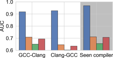
(a) Function Similarity

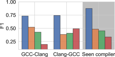
(b) Function Signature

Figure 2: Comparing SymC and baselines on samples compiled by different compilers across different binary analysis tasks (§6.4).

Unseen compilers. We conduct two sets of experiments: training on GCC-compiled binaries and evaluating on Clang-compiled binaries (GCC-Clang), and vice versa (Clang-GCC). Additionally, we include the experiment with the same compiler for both training and testing, i.e., Clang-Clang and GCC-GCC, as the reference. Memory region prediction is not included due to missing compiler information in the dataset from DeepVSA [32].

Figure 2 shows that SymC consistently outperforms PalmTree on unseen compilers (e.g., 38.6% on function signature prediction). On seen compilers (marked in gray), SymC achieves even better performance with a larger margin (at least 44.6% higher). Note that all the results obtained from SymC do not require any pre-training effort.

Unseen optimizations. We vary the compiler optimizations in training and evaluation and include reference experiments where the training and evaluation share the same optimization options (marked in gray). For function similarity detection, training on O0-O1 means the function pair has one function compiled with O0 and the other with O1. In the case of evaluating on unseen optimizations, the corresponding testing set has to come from those compiled with O2-O3 to ensure the optimizations are unseen.

Figure 3 shows that SymC outperforms PalmTree by 31% when evaluated on unseen optimizations. SymC experiences a performance drop (e.g., by 28.6%) when not trained on O0 but tested on those compiled with O0. We believe this drop is caused by the extensive optimizations already enabled at the O1 (e.g., GCC employs 47 optimizations to aggressively reduce execution time and code size). The shift in distribution between O1 and O0 is much more pronounced than between O2 and O1, indicated by a KL divergence of 1.56 from O1 to O0 compared to 0.06 (96.2% lower) from O3 to O2. Nevertheless, when evaluated on seen optimizations, SymC outperforms PalmTree by 28.1% on average.

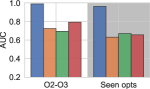
(a) Train on O0-O1

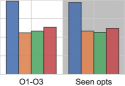
(b) Train on O0-O2

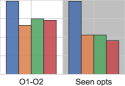
(c) Train on O0-O3

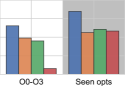
(d) Train on O1-O2

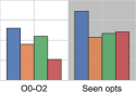
(e) Train on O1-O3

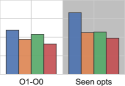
(f) Train on O2-O3

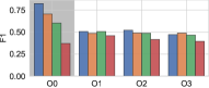
(g) Train on O0

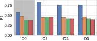
(h) Train on O1

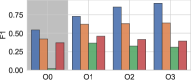
(i) Train on O2

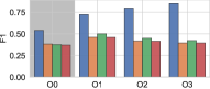
(j) Train on O3

Figure 3: Unseen optimization evaluation. The upper row, i.e., (a)-(f), shows the results on function similarity detection. The lower row, i.e., (g)-(j), are results on function signature prediction. We also include the evaluation on seen optimizations (marked in gray).

Unseen obfuscations. We compare SymC to baselines on generalization to unseen obfuscations. Figure 4 shows that SymC outperforms PalmTree (on average) on unseen and seen obfuscations by 33.3% and 36.6%, respectively. Similar to the observations in evaluating unseen optimizations, while the obfuscations are not directly related to instruction permutations (i.e., automorphisms in $Aut(PDG)$), SymC maintains its superior performance.

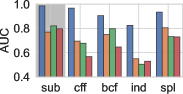
(a) Train on sub

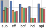
(b) Train on cff

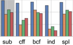
(c) Train on bcf

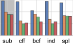
(d) Train on ind

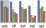
(e) Train on spl

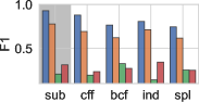
(f) Train on sub

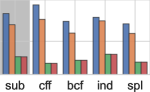
(g) Train on cff

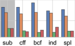
(h) Train on bcf

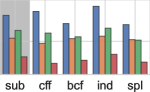
(i) Train on ind

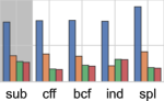
(j) Train on spl

Figure 4: Unseen obfuscations evaluation. Similar to Figure 3, the upper row, i.e., (a)-(e), shows the results on function similarity detection. The lower row, i.e., (f)-(j), are results on function signature prediction. We also include the evaluation on seen optimizations (marked in gray).

Unseen permutations. We evaluate SymC and baselines on permuted testing samples that respect $Aut(PDG)$. Using a topological sorting [40], we group permutable instructions while preserving their relative order based on PDG edges. Varying the number of groups controls the percentage of permutations. Table I shows that SymC outperforms all baselines at all permutation percentages, e.g., beat PalmTree by 40.5%. Moreover, SymC remains stable across all percentages of the permutations, while the baselines suffer from nontrivial performance drops, e.g., by 26.6% for PalmTree.

TABLE I: Evaluation on unseen permutations. We include the evaluation on original samples (0%) for comparison.

		0%	25%	50%	75%	100%	Avg.
Function Similarity	SymC	0.96	0.96	0.96	0.96	0.96	0.96
	PalmTree	0.57	0.45	0.45	0.48	0.43	0.48
	PalmTree-O	0.57	0.42	0.45	0.47	0.44	0.47
	PalmTree-N	0.32	0.22	0.29	0.17	0.2	0.24
Function Signature	SymC	0.88	0.88	0.88	0.88	0.88	0.88
	PalmTree	0.59	0.55	0.49	0.42	0.41	0.49
	PalmTree-O	0.49	0.48	0.45	0.41	0.41	0.45
	PalmTree-N	0.19	0.41	0.41	0.41	0.41	0.37
Memory Region	SymC	0.86	0.86	0.86	0.86	0.86	0.86
	PalmTree	0.57	0.45	0.45	0.48	0.43	0.48
	PalmTree-O	0.57	0.42	0.45	0.47	0.44	0.47
	PalmTree-N	0.32	0.22	0.29	0.17	0.2	0.24
Function Name	SymC	0.57	0.56∗	0.57	0.57	0.57	0.57
	code2seq	0.33	0.33	0.33	0.33	0.33	0.33
	code2vec	0.33	0.32	0.33	0.32	0.32	0.32
	GGNN	0.41	0.41	0.41	0.41	0.42	0.41
∗We observe a slight value change due to the floating point precision error resulting from limited model weight precision (16-bit) as mentioned in §6.5.

Unseen lengths. We assess SymC’s generalizability on longer sequences than those seen in training, a common task for evaluating model generalizability [29]. We divide samples into four length bins (bin1 to bin4) based on their distribution in the dataset (§6.3). The bins are non-overlapping and increase in length. For example, we used bins [0-10], [1-20], [21-50], and [51-500] for function similarity detection. Figure 5 demonstrates that SymC is 41.8% better than PalmTree in generalizing to longer lengths.

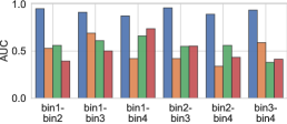
(a) Function similarity

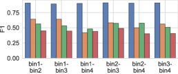
(b) Function signature

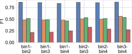
(c) Memory region

Figure 5: Evaluation on unseen longer lengths, where bin1-bin4 denote training on samples with lengths in bin1 and testing on those in bin4.

Unseen source code transformations. We evaluate SymC against the source code baselines (§6.2) on different unseen source code transformations (§6.4). We control the percentage of the transformations following the similar practice in statement permutations. Table II shows that SymC outperforms code2seq, code2vec and GGNN, by 48.9%, 53.6%, and 36.7%, respectively, across all percentages of transformations applied. We observe that the F1 scores of the baselines across different transformation percentages do not vary much. We thus check the prediction of these baselines before and after the transformation and notice the predicted labels change significantly, e.g., on average 49.9% of the predicted labels change. However, as the changes are mainly from one incorrectly predicted label to another incorrect prediction, this does not lead to the significant change in F1, e.g., code2seq remains at 0.33 (with $\pm 0.005$) across all permutation percentages. By contrast, SymC remains invariant in both predicted labels and F1 scores.

TABLE II: Evaluation on unseen source code transformations varied by how much percentage of transformations.

		0%	25%	50%	75%	100%	Avg.
Variable Renaming	SymC	0.57	0.59	0.59	0.58	0.59	0.58
	code2seq	0.34	0.31	0.33	0.3	0.3	0.32
	code2vec	0.29	0.31	0.32	0.28	0.29	0.3
	GGNN	0.37	0.36	0.38	0.36	0.38	0.37
Statement Permutation	SymC	0.57	0.56	0.57	0.57	0.57	0.57
	code2seq	0.33	0.33	0.33	0.33	0.33	0.33
	code2vec	0.33	0.32	0.33	0.32	0.32	0.32
	GGNN	0.41	0.41	0.41	0.41	0.42	0.41
Loop Exchange	SymC	0.62	0.6	0.61	0.6	0.61	0.61
	code2seq	0.27	0.3	0.27	0.3	0.27	0.28
	code2vec	0.27	0.24	0.27	0.24	0.27	0.26
	GGNN	0.34	0.32	0.34	0.32	0.34	0.33
Boolean Exchange	SymC	0.62	0.59	0.62	0.59	0.62	0.61
	code2seq	0.31	0.25	0.31	0.25	0.3	0.28
	code2vec	0.25	0.19	0.24	0.18	0.22	0.22
	GGNN	0.47	0.31	0.44	0.31	0.43	0.39

7.2 RQ2: Efficiency

Besides improved generalization to unseen transformed samples, the symmetry-preserving design of SymC significantly improves training efficiency by avoiding expensive pre-training efforts, e.g., some may take up to 10 days [38, 60]. As shown in §7.1, SymC, without any pre-training, outperforms the pre-trained baselines.

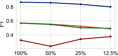
(a) Reduce model size

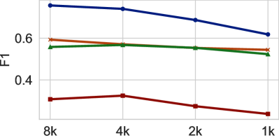
(b) Reduce training iterations

Figure 6: Comparing SymC and baselines on constrained resources, where we (a) reduce the model weights, and (b) reduce the number of training iterations, and observe how that affects the performance.

In this section, we focus on evaluating the training efficiency of SymC. We first assess SymC’s performance against the baselines under limited training resources, where we reduce the model sizes and training iterations, with the hypothesis that SymC requires less training effort for similar testing performance due to its improved training efficiency. Figure 6 shows that SymC’s memory region prediction performance remains the highest in both reduced size and training iterations, e.g., by 36.9% and 21.4% better than PalmTree on average. Even in the most strict scenario, SymC remains 38.2% and 15.3% better in both settings.

TABLE III: The resource consumed by training SymC and other baselines to reach 0.5 F1 score in memory region prediction.

	GPU Time (Hours)	Power Usage (kWh)	Carbon Emitted (CO2eq)
SymC	0.07	0.025	0.009
PalmTree-O∗	89.67	31.38	11.64
∗ PalmTree did not disclose its hours for pre-training, so we include the pre- training time (in 10 epochs) based on our own pre-trained PalmTree.

Besides the constrained resource, we evaluate the training effort of SymC and PalmTree (including both pre-training and fine-tuning). Table III shows their GPU hours, power, and emitted carbon dioxide estimation when they reach 0.5 F1 score in memory region prediction. We assume the GPU always reaches its power cap (350W for GTX 3090) to estimate an upper bound of the power usage. CO₂eq stands for the carbon dioxide equivalent, a unit for measuring carbon footprints, and the current emission factor is 0.371 CO₂eq per kWh [24]. By being more training efficient, SymC incurs 1,281$\times$ less total GPU time, power, and emitted carbon dioxide than PalmTree in obtaining the same performance.

7.3 RQ3: Ablations

In this section, we aim to study how several design choices made in SymC compare to the potential alternatives.

Equivariance vs. Invariance. We compare the $Aut(PDG)$-equivariant self-attention layers in SymC to the $Aut(PDG)$-invariant ones. Specifically, we investigate the impact of making self-attention invariant in the early layers, i.e., 2nd, 4th, or 6th layer. We omit considering the other layers as we observe small performance discrepancies between neighboring layers. Figure 7a shows that setting layers invariant early hinders analysis performance, i.e., SymC with equivariant layers has 0.73 F1 score on average across all training iterations, and outperforms the setting of invariant from 6th layer by 60.7%.

Pre-training benefit. We explore the impact of pre-training SymC with masked language modeling [50, 17] on downstream tasks. Figure 7b compares SymC without pre-training to pre-trained versions with varying iterations for memory region prediction. Pre-training with even one epoch results in a significantly improved F1 score, e.g., by 10.8%, with much faster convergence. However, additional pre-training epochs show diminishing returns, likely due to the limited training samples, e.g., the F1 score only improves by 3.2% with pre-training five epochs compared to 1 epoch.

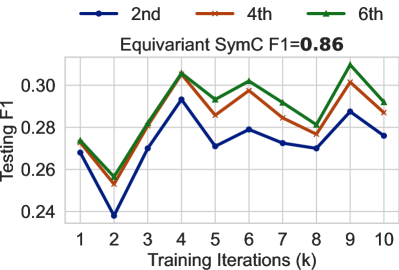
(a) Equivariance vs. Invariance

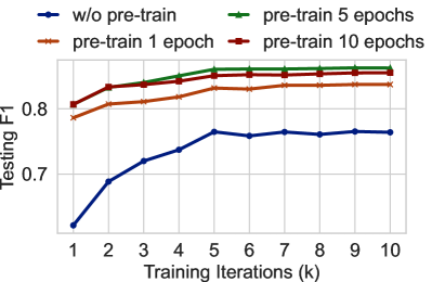
(b) Pre-training SymC

Figure 7: (a) Comparing SymC’s equivariant self-attention layers with setting its layers invariant starting at earlier layer. (b) Comparing SymC (not pre-trained) to pre-trained SymC with various pre-training epochs.

8 Limitations & Future Work

SymC can be further improved in several directions. First, by exploring symmetry-aware pre-training, we can identify semantically equivalent symmetry-transformed samples [77], reducing the number of required pre-training samples and potentially improving the model’s efficiency.

Second, considering various symmetries beyond automorphisms, such as permutations at the whole x64 assembly instruction set level, allows SymC to support instruction addition, deletion, and replacement. This capability is beneficial in malware analysis, where code is often transformed using obfuscations involving these types of substitutions.

Finally, expanding SymC to other architectures, such as convolutional networks and graph neural networks, or developing new architectures better suited for specific program symmetry groups, can also present exciting opportunities.

9 Related Work

Code representation learning. Previous research aims to automate software development tasks through code representation learning [51]. Recent works focus on generalizable program representations for various code reasoning tasks [19, 21, 2, 57, 47, 59, 41, 26, 54, 22, 30, 1, 31], employing new architectures and pre-training objectives [33, 3, 27, 73, 61, 42, 62, 31]. However, these approaches rely solely on empirical evidence for semantic encoding. By contrast, this paper introduces a formal group-theoretic framework to quantify learned program semantics through invariance/equivariance against symmetry groups.

Symmetry in machine learning. Symmetry plays a crucial role in creating efficient neural architectures across various domains [66, 11, 63, 64, 15, 29]. Different architectures, such as CNNs, graph neural nets, and Transformers, leverage symmetry to handle translations, rotations, and permutations [44, 15, 25, 29, 67]. However, SymC is the first to formalize code semantics learning using semantics-preserving symmetry groups.

10 Conclusion

We studied code symmetries’ impact on code LLM architectures for program reasoning tasks, introducing a novel self-attention variant that brought significant gains in generalization and robustness across a variety of program analysis tasks, providing valuable insights for specialized LLM development in reasoning and analyzing programs.

Appendix A Self-Attention Background

Given the embeddings of all vertices $f_{i}$ from $\mathcal{IG}$, we consider a sequence of embeddings by flattening $\mathcal{IG}$ following the order of instructions in $c$. Let this sequence of embeddings be denoted as $e=(e_{1},...,e_{n})$. The self-attention computation, denoted as $A$, takes $e$ as input and produces another sequence of embeddings, denoted as $(e^{\prime}_{1},...,e^{\prime}_{n})$.

The core operations in self-attention $A$ involve updating each embedding $e_{i}$ through the following steps:

1. First, it maps each embedding $e_{i}$ to three embeddings (query, key, and value): $q_{i}=f_{q}(e_{i})$, $k_{i}=f_{k}(e_{i})$, $v_{i}=f_{v}(e_{i})$, where $f_{q}$, $f_{k}$, and $f_{v}$ are affine transformations (i.e., fully-connected linear layers) parameterized by $w_{q}$, $w_{k}$, and $w_{v}$, respectively.

2. Next, it computes the attention score $a_{ij}$ between every pair of embeddings $e_{i}$ and $e_{j}$ by taking the dot product between the query $q_{i}$ of $e_{i}$ and the key $k_{j}$ of $e_{j}$: $a_{ij}=q_{i}\cdot k_{j}$. The attention scores form a square matrix, where each cell $a_{ij}$ indicates the attention that $e_{i}$ should pay to $e_{j}$. The attention scores are then divided by $\sqrt{d}$ (the dimension of the embedding vectors), scaled using the softmax function to ensure they sum up to 1: $\hat{a}_{ij}=\frac{\exp(a{ij})}{\sum^{n}_{j=1}\exp(a_{ij})}$. These two operations are denoted by $s$.

3. Finally, the scaled attention score $\hat{a}_{ij}$ is multiplied by $v_{j}$, and a vector sum is computed: $e^{\prime}_{i}=\sum^{n}_{j=1}\hat{a}_{ij}v_{ij}$.

Appendix B Proofs

Lemma 1. Let $f_{1}$ and $f_{2}$ be two functions that are both $G$-equivariant and $h=f_{1}\circ f_{2}$ be the new function composed by $f_{1}$ and $f_{2}$. $h$ is also $G$-equivariant.

• For all $g\in G$ and any input $x$, we have

  $$h(g\circ x) =(f_{1}\circ f_{2})(g\circ x)$$

  $$=f_{1}(f_{2}(g\circ x)) \triangleright$$ Associativity

  $$=f_{1}(g\circ f_{2}(x)) \triangleright f_{2} g$$ is equivariant to

  $$=g\circ f_{1}(f_{2}(x)) \triangleright f_{1} g$$ is equivariant to

  $$=g\circ(f_{1}\circ f_{2})(x) \triangleright$$ Associativity

  $$=g\circ h(x)$$

  Therefore, $h(g\circ x)=g\circ h(x)$, so $h$ is $G$-equivariant.

Lemma 2. Let $f_{1}$ and $f_{2}$ be two functions where $f_{1}$ is $G$-equivariant $f_{2}$ is $G$-invariant, and $h=f_{2}\circ f_{1}$ be the new function composed by applying $f_{1}$ and then $f_{2}$. $h$ is $G$-invariant.

For all $g\in G$ and any input $x$, we have

$$h(g\circ x) =(f_{2}\circ f_{1})(g\circ x)$$

$$=f_{2}(f_{1}(g\circ x)) \triangleright$$ Associativity

$$=f_{2}(g\circ f_{1}(x)) \triangleright f_{1} g$$ is equivariant to

$$=f_{2}(f_{1}(x)) \triangleright f_{2} g$$ is invariant to

$$=(f_{2}\circ f_{1})(x) \triangleright$$ Associativity

$$=h(x)$$

Theorem 1. The set of automorphisms $\sigma\in Aut(\mathcal{IG})$ forms a program symmetry group.

• Consider an arbitrary $\sigma\in Aut(\mathcal{IG})$. Definition 4.8 states that for all $f_{i}\in\{f_{1},...,f_{n}\}$, $\sigma(f_{i})$ have the same edges as $\mathcal{IG}$ before $\sigma$ was applied. As $\sigma$ is a permutation and there is also a bijective mapping between $f_{i}$ and $c_{i}$, i.e., $f_{i}$ always interprets $c_{i}$, we have $\sigma(f_{i})=f_{i}(\sigma\circ c_{i},in_{i})$. Definition 4.8 also states that $\sigma(f_{i})$ is connected with the same edges. Therefore, the output of $\sigma(f_{i})=out_{i}$. We thus have $f_{i}(\sigma\circ c_{i},in_{i})=out_{i}=f_{i}(c_{i},in_{i}),\forall\sigma\in Aut(\mathcal{IG})$ and $\forall f_{i}\in\{f_{1},...,f_{n}\}$. Therefore, all $\sigma\in Aut(\mathcal{IG})$ are semantics-preserving program symmetries, according to Definition 4.6. Moreover, it is well known in the literature that the automorphisms of any graph form a group by satisfying group axioms (Definition 3.1) [10, 78]. Therefore, $Aut(\mathcal{IG})$ forms a group of program symmetries, according to Definition 4.7: $Aut(\mathcal{IG})\in G$.

Lemma 3. Embedding layer $Emb$ is $Aut(\mathcal{IG})$-equivariant.

• Let us formally define the embedding layer $Emb$. It maps each vertex $f_{i}$ in the graph $\mathcal{IG}$ to an embedding vector $e_{i}\in\mathbb{R}^{d}$. Given the set of vertices $V_{\mathcal{IG}}={f_{1},...,f_{n}}$, the embedded vertices are denoted as $Emb(V_{\mathcal{IG}})={Emb(f_{1}),...,Emb(f_{n})}$.

  Now, let $\sigma$ be an automorphism, which is a bijective function from ${f_{1},...,f_{n}}$ to itself. When $\sigma$ acts on the set of vertices ${f_{1},...,f_{n}}$, we define the permuted vertices as ${f_{\sigma(1)},f_{\sigma(2)},...,f_{\sigma(n)}}$.

  To prove $Emb$ is $Aut(\mathcal{IG})$-equivariant, we need to show that $Emb(\sigma(V_{\mathcal{IG}}))=\sigma(Emb(V_{\mathcal{IG}}))$.

  When applying $\sigma$ to the set of vertices, we have $\sigma(V_{\mathcal{IG}})={f_{\sigma(1)},...,f_{\sigma(n)}}$. Applying $Emb$ to this permuted set of vertices, we obtain $Emb(\sigma(V_{\mathcal{IG}}))={Emb(f_{\sigma(1)}),...,Emb(f_{\sigma(n)})}$. On the other hand, applying $\sigma$ to the set of embedded vertices, we have $\sigma(Emb(V_{\mathcal{IG}}))={\sigma(Emb(f_{1})),...,\sigma(Emb(f_{n}))}$.

  Since $\sigma$ is an automorphism, it preserves the ordering of the embedded vertices. Therefore, $\sigma(Emb(f_{i}))=Emb(f_{\sigma(i)})$ for each $i$. Thus, we have $\sigma(Emb(V_{\mathcal{IG}}))={Emb(f_{\sigma(1)}),...,Emb(f_{\sigma(n)})}$. Therefore, we can conclude that $Emb(\sigma(V_{\mathcal{IG}}))=\sigma(Emb(V_{\mathcal{IG}}))$. Hence, the embedding layer $Emb$ is $Aut(\mathcal{IG})$-equivariant.

Lemma 4. The biased self-attention layer computing the embedding $e^{\prime}_{i}=GA(e_{i})$ is $Aut(\mathcal{IG})$-invariant.

$$e^{\prime}_{i} =GA(\sigma\cdot e_{i})$$

$$=w_{v}\sigma(e)\cdot(s(w_{k}\sigma(e)^{T}\cdot w_{q}e_{i})+\sigma(d_{i}))$$

$$d_{i} d_{i} p^{T}_{\sigma}d_{i}$$ is a column vector, so permuting the row of is achieved by (see §4.4):

$$=w_{v}ep_{\sigma}\cdot(s((w_{k}ep_{\sigma})^{T}\cdot w_{q}e_{i})+p^{T}_{\sigma}d_{i})$$

$$=w_{v}ep_{\sigma}\cdot s(p_{\sigma}^{T}(w_{k}e)^{T}\cdot w_{q}e_{i})+w_{v}ep_{\sigma}\cdot p^{T}_{\sigma}d_{i}$$

$$=w_{v}e(p_{\sigma}p_{\sigma}^{T})\cdot s((w_{k}e)^{T}\cdot w_{q}e_{i})+w_{v}e\cdot(p_{\sigma}p^{T}_{\sigma})\cdot d_{i}$$

$$p_{\sigma}$$ is an orthogonal matrix (see §4.4):

$$=w_{v}e\cdot((s(w_{k}e)^{T}\cdot w_{q}e_{i})+d_{i})$$

$$=GA(e_{i})$$

Lemma 5. The distance matrix $d$ of PDG remains invariant under the action of $\sigma\in Aut(PDG)$.

• We need to show that the shortest path $p_{\sigma(i)\sigma(j)}$ from $\sigma(T_{ij})$ to $\sigma(V_{i})$ remains the same as $p_{ij}$ (the same applies to $n_{\sigma(i)\sigma(j)}$). Without loss of generality, we focus on proving $p_{\sigma(i)\sigma(j)}=p_{ij}$.

  Assume there exists a shortest path $P=(T_{ij},...,V_{i})$. Let $P^{\prime}=(\sigma(T_{ij}),...,\sigma(V_{i}))$ be the corresponding shortest path in $\sigma(PDG)$ under the automorphism $\sigma$. We need to demonstrate two properties.

  First, $P^{\prime}$ is a valid path from $\sigma(T_{ij})$ to $\sigma(V_{i})$. Since $P$ is a valid path, $T_{ij}$ is adjacent to its next node in $P$ (denoted as $V_{m}$), and this holds for every pair of neighboring nodes until $V_{i}$. As $\sigma$ is an automorphism, the same adjacency relationship holds for $P^{\prime}$, where $\sigma(T_{ij})$ is adjacent to $\sigma(V_{m})$ and so on, until $\sigma(V_{i})$. Hence, $P^{\prime}$ is a valid path from $\sigma(T_{ij})$ to $\sigma(V_{i})$ in PDG.

  Second, we aim to show that $|P|=|P^{\prime}|$, meaning $p_{\sigma(i)\sigma(j)}=p_{ij}$. Suppose, for contradiction, that $p_{\sigma(i)\sigma(j)}\neq p_{ij}$. Let’s consider the case where $p_{\sigma(i)\sigma(j)}<p_{ij}$. This implies that the length of the path $P^{\prime}=(\sigma(T_{ij}),\sigma(V_{m}),...,\sigma(V_{n}),\sigma(V_{i}))$ is shorter than $p_{ij}$.

  Now, let’s apply $\sigma^{-1}$ to each node in $P^{\prime}$, resulting in $\sigma^{-1}(P^{\prime})$. Since $\sigma^{-1}$ is also in $Aut(PDG)$ and $\sigma^{-1}(\sigma(V))=V$ (Definition 3.1), each pair of adjacent nodes in $P^{\prime}$, after applying $\sigma^{-1}$, remains adjacent. Furthermore, the path formed by these adjacent nodes has a length of $p_{\sigma(i)\sigma(j)}$, connecting $T_{ij}$ and $V_{i}$ in the original PDG.

  Therefore, we obtain a path in PDG connecting $T_{ij}$ and $V_{i}$ that is shorter than $p_{ij}$, contradicting the fact that $p_{ij}$ is the shortest path in PDG between $T_{ij}$ and $V_{i}$. Thus, we reject the assumption that $p_{\sigma(i)\sigma(j)}<p_{ij}$.

  Similarly, we can prove that $p_{\sigma(i)\sigma(j)}>p_{ij}$ is also false by demonstrating its contradiction with the fact that $p_{\sigma(i)\sigma(j)}$ is the shortest path in $\sigma(PDG)$.

  Hence, we conclude that $p_{\sigma(i)\sigma(j)}=p_{ij}$, and as a result, the positive distance matrix $dp$ remains invariant under the action of $\sigma\in Aut(PDG)$.

  By following the same steps, we can prove that $n_{\sigma(i)\sigma(j)}=n_{ij}$, demonstrating the invariance of the negative distance matrix $dn$ under the action of $\sigma\in Aut(PDG)$.

  Therefore, the distance matrix $d$ remains invariant.

Lemma 6. The distance matrix $d$ of $PDG$ commutes with permutation matrix $p_{\sigma}$ of the automorphism $\sigma\in Aut(PDG)$: $d\cdot p_{\sigma}=p_{\sigma}\cdot d$.

• According to Lemma 5, we have:

  $$p^{T}_{\sigma}\cdot d\cdot p_{\sigma} =d$$

  $$p_{\sigma}\cdot p^{T}_{\sigma}\cdot d\cdot p_{\sigma} =p_{\sigma}\cdot d \triangleright p_{\sigma}$$ Apply on both side

  $$d\cdot p_{\sigma} =p_{\sigma}\cdot d \triangleright p_{\sigma}$$ is orthogonal matrix

Lemma 7. The sum of the input embedding tokens sequences is $Aut(PDG)$-equivariant: $Emb(\sigma\circ x)=\sigma\circ Emb(x)$.

• According to Lemma 3, we can prove that each of these four embeddings is $Aut(PDG)$-equivariant. Therefore, we have $Emb(x)=Emb_{c}(\sigma\circ x_{c})+Emb_{pos}(\sigma\circ x_{pos})+Emb_{ind}(\sigma\circ x_{ind})+Emb_{outd}(\sigma\circ x_{outd})=\sigma\circ Emb_{c}(x_{c})+\sigma\circ Emb_{pos}(x_{pos})+\sigma\circ Emb_{ind}(x_{ind})+\sigma\circ Emb_{outd}(x_{outd})$. Similar to the idea that multi-head self-attention layer operates on the per embedding level regardless of the position of each token’s position in the sequence, here the sum is a linear operation that also performs per embedding sum across the 4 embedding sequences. Therefore, we have $Emb(\sigma\circ x)=\sigma\circ Emb_{c}(x_{c})+\sigma\circ Emb_{pos}(x_{pos})+\sigma\circ Emb_{ind}(x_{ind})+\sigma\circ Emb_{outd}(x_{outd})=\sigma\circ(Emb_{c}(x_{c})+Emb_{pos}(x_{pos})+Emb_{ind}(x_{ind})+Emb_{outd}(x_{outd}))=\sigma\circ Emb(x)$.

Lemma 8.

Standard self-attention layer $A$ is equivariant to the group of all permutations of input sequences.

Based on the operations performed by the self-attention layer and the permutation matrix, we can show the equivariance property as follows [37]:

$$A (\pi\cdot e)$$

$$=w_{v}\pi(e)\cdot s(w_{k}\pi(e)^{T}\cdot w_{q}\pi(e))$$

$$=w_{v}ep_{\pi}\cdot s((w_{k}ep_{\pi})^{T}\cdot w_{q}ep_{\pi}) \triangleright p_{\pi}$$ Applying

$$=w_{v}ep_{\pi}\cdot s(p_{\pi}^{T}(w_{k}e)^{T}\cdot w_{q}ep_{\pi}) \triangleright$$ Transpose of a product

$$=w_{v}e(p_{\pi}p_{\pi}^{T})\cdot s((w_{k}e)^{T}\cdot w_{q}e)p_{\pi}$$

$$=w_{v}e\cdot s((w_{k}e)^{T}\cdot w_{q}e)p_{\pi} \triangleright p_{\pi}$$ is orthogonal matrix

$$=\pi(A(e))$$

References

- [1] W. U. Ahmad, S. Chakraborty, B. Ray, and K.-W. Chang, “Unified pre-training for program understanding and generation,” arXiv preprint arXiv:2103.06333, 2021.
- [2] M. Allamanis, E. T. Barr, P. Devanbu, and C. Sutton, “A survey of machine learning for big code and naturalness,” ACM Computing Surveys (CSUR), vol. 51, no. 4, pp. 1–37, 2018.
- [3] M. Allamanis, M. Brockschmidt, and M. Khademi, “Learning to represent programs with graphs,” arXiv preprint arXiv:1711.00740, 2017.
- [4] M. Allamanis, H. Peng, and C. Sutton, “A convolutional attention network for extreme summarization of source code,” in International conference on machine learning. PMLR, 2016, pp. 2091–2100.
- [5] U. Alon, S. Brody, O. Levy, and E. Yahav, “code2seq: Generating sequences from structured representations of code,” arXiv preprint arXiv:1808.01400, 2018.
- [6] U. Alon, M. Zilberstein, O. Levy, and E. Yahav, “code2vec: Learning distributed representations of code,” Proceedings of the ACM on Programming Languages, vol. 3, no. POPL, pp. 1–29, 2019.
- [7] D. Arp, E. Quiring, F. Pendlebury, A. Warnecke, F. Pierazzi, C. Wressnegger, L. Cavallaro, and K. Rieck, “Dos and don’ts of machine learning in computer security,” in 31st USENIX Security Symposium (USENIX Security 22), 2022, pp. 3971–3988.
- [8] F. Artuso, M. Mormando, G. A. Di Luna, and L. Querzoni, “Binbert: Binary code understanding with a fine-tunable and execution-aware transformer,” arXiv preprint arXiv:2208.06692, 2022.
- [9] P. Banerjee, K. K. Pal, F. Wang, and C. Baral, “Variable name recovery in decompiled binary code using constrained masked language modeling,” arXiv preprint arXiv:2103.12801, 2021.
- [10] N. Biggs, N. L. Biggs, and B. Norman, Algebraic graph theory. Cambridge university press, 1993, no. 67.
- [11] A. Bogatskiy, B. Anderson, J. Offermann, M. Roussi, D. Miller, and R. Kondor, “Lorentz group equivariant neural network for particle physics,” in International Conference on Machine Learning. PMLR, 2020, pp. 992–1002.
- [12] J. Bundt, M. Davinroy, I. Agadakos, A. Oprea, and W. Robertson, “Black-box attacks against neural binary function detection,” arXiv preprint arXiv:2208.11667, 2022.
- [13] Q. Chen, J. Lacomis, E. J. Schwartz, C. Le Goues, G. Neubig, and B. Vasilescu, “Augmenting decompiler output with learned variable names and types,” in 31st USENIX Security Symposium (USENIX Security 22), 2022, pp. 4327–4343.
- [14] Z. L. Chua, S. Shen, P. Saxena, and Z. Liang, “Neural nets can learn function type signatures from binaries,” in 26th USENIX Security Symposium, 2017.
- [15] T. Cohen and M. Welling, “Group equivariant convolutional networks,” in International conference on machine learning. PMLR, 2016, pp. 2990–2999.
- [16] C. Deshpande, D. Gens, and M. Franz, “Stackbert: Machine learning assisted static stack frame size recovery on stripped and optimized binaries,” in Proceedings of the 14th ACM Workshop on Artificial Intelligence and Security, 2021, pp. 85–95.
- [17] J. Devlin, M.-W. Chang, K. Lee, and K. Toutanova, “Bert: Pre-training of deep bidirectional transformers for language understanding,” arXiv preprint arXiv:1810.04805, 2018.
- [18] S. H. Ding, B. C. Fung, and P. Charland, “Asm2vec: Boosting static representation robustness for binary clone search against code obfuscation and compiler optimization,” in 2019 IEEE Symposium on Security and Privacy (SP). IEEE, 2019, pp. 472–489.
- [19] Y. Ding, S. Chakraborty, L. Buratti, S. Pujar, A. Morari, G. Kaiser, and B. Ray, “Concord: Clone-aware contrastive learning for source code,” arXiv preprint arXiv:2306.03234, 2023.
- [20] Y. Ding, B. Steenhoek, K. Pei, G. Kaiser, W. Le, and B. Ray, “Traced: Execution-aware pre-training for source code,” arXiv preprint arXiv:2306.07487, 2023.
- [21] Y. Ding, Z. Wang, W. U. Ahmad, M. K. Ramanathan, R. Nallapati, P. Bhatia, D. Roth, and B. Xiang, “Cocomic: Code completion by jointly modeling in-file and cross-file context,” arXiv preprint arXiv:2212.10007, 2022.
- [22] E. Downing, Y. Mirsky, K. Park, and W. Lee, “DeepReflect: Discovering malicious functionality through binary reconstruction,” in 30th USENIX Security Symposium (USENIX Security 21), 2021, pp. 3469–3486.
- [23] M. Egele, T. Scholte, E. Kirda, and C. Kruegel, “A survey on automated dynamic malware-analysis techniques and tools,” ACM computing surveys (CSUR), vol. 44, no. 2, pp. 1–42, 2008.
- [24] EPA, “Emission Factors for Greenhouse Gas Inventories,” https://www.epa.gov/system/files/documents/2022-04/ghg_emission_factors_hub.pdf, 2022.
- [25] C. Esteves, C. Allen-Blanchette, A. Makadia, and K. Daniilidis, “Learning so (3) equivariant representations with spherical cnns,” in Proceedings of the European Conference on Computer Vision (ECCV), 2018, pp. 52–68.
- [26] Z. Feng, D. Guo, D. Tang, N. Duan, X. Feng, M. Gong, L. Shou, B. Qin, T. Liu, D. Jiang et al., “Codebert: A pre-trained model for programming and natural languages,” arXiv preprint arXiv:2002.08155, 2020.
- [27] P. Fernandes, M. Allamanis, and M. Brockschmidt, “Structured neural summarization,” arXiv preprint arXiv:1811.01824, 2018.
- [28] F. Gao, Y. Wang, and K. Wang, “Discrete adversarial attack to models of code,” Proceedings of the ACM on Programming Languages, vol. 7, no. PLDI, pp. 172–195, 2023.
- [29] J. Gordon, D. Lopez-Paz, M. Baroni, and D. Bouchacourt, “Permutation equivariant models for compositional generalization in language,” in International Conference on Learning Representations, 2019.
- [30] D. Guo, S. Lu, N. Duan, Y. Wang, M. Zhou, and J. Yin, “Unixcoder: Unified cross-modal pre-training for code representation,” arXiv preprint arXiv:2203.03850, 2022.
- [31] D. Guo, S. Ren, S. Lu, Z. Feng, D. Tang, S. Liu, L. Zhou, N. Duan, A. Svyatkovskiy, S. Fu et al., “Graphcodebert: Pre-training code representations with data flow,” arXiv preprint arXiv:2009.08366, 2020.
- [32] W. Guo, D. Mu, X. Xing, M. Du, and D. Song, “DEEPVSA: Facilitating value-set analysis with deep learning for postmortem program analysis,” in 28th USENIX Security Symposium (USENIX Security 19), 2019.
- [33] V. J. Hellendoorn, C. Sutton, R. Singh, P. Maniatis, and D. Bieber, “Global relational models of source code,” in International conference on learning representations, 2019.
- [34] J. Henke, G. Ramakrishnan, Z. Wang, A. Albarghouth, S. Jha, and T. Reps, “Semantic robustness of models of source code,” in 2022 IEEE International Conference on Software Analysis, Evolution and Reengineering (SANER). IEEE, 2022, pp. 526–537.
- [35] I. Higgins, D. Amos, D. Pfau, S. Racaniere, L. Matthey, D. Rezende, and A. Lerchner, “Towards a definition of disentangled representations,” arXiv preprint arXiv:1812.02230, 2018.
- [36] J. Hu, Q. Zhang, and H. Yin, “Augmenting greybox fuzzing with generative ai,” arXiv preprint arXiv:2306.06782, 2023.
- [37] S. Ji, Y. Xie, and H. Gao, “A mathematical view of attention models in deep learning,” Texas A&M University: College Station, TX, USA, 2019.
- [38] X. Jin, K. Pei, J. Y. Won, and Z. Lin, “Symlm: Predicting function names in stripped binaries via context-sensitive execution-aware code embeddings,” in Proceedings of the 2022 ACM SIGSAC Conference on Computer and Communications Security, 2022, pp. 1631–1645.
- [39] N. Jovanovic, C. Kruegel, and E. Kirda, “Pixy: A static analysis tool for detecting web application vulnerabilities,” in 2006 IEEE Symposium on Security and Privacy (S&P’06). IEEE, 2006, pp. 6–pp.
- [40] A. B. Kahn, “Topological sorting of large networks,” Communications of the ACM, vol. 5, no. 11, pp. 558–562, 1962.
- [41] H. Kim, J. Bak, K. Cho, and H. Koo, “A transformer-based function symbol name inference model from an assembly language for binary reversing,” in Proceedings of the 2023 ACM Asia Conference on Computer and Communications Security, 2023, pp. 951–965.
- [42] S. Kim, J. Zhao, Y. Tian, and S. Chandra, “Code prediction by feeding trees to transformers,” in 2021 IEEE/ACM 43rd International Conference on Software Engineering (ICSE). IEEE, 2021, pp. 150–162.
- [43] D. Knuth, “Permutations, matrices, and generalized young tableaux,” Pacific journal of mathematics, vol. 34, no. 3, pp. 709–727, 1970.
- [44] Y. LeCun, Y. Bengio, and G. Hinton, “Deep learning,” nature, vol. 521, no. 7553, pp. 436–444, 2015.
- [45] Y. J. Lee, S.-H. Choi, C. Kim, S.-H. Lim, and K.-W. Park, “Learning binary code with deep learning to detect software weakness,” in KSII the 9th international conference on internet (ICONI) 2017 symposium, 2017.
- [46] H. Li, Y. Hao, Y. Zhai, and Z. Qian, “The hitchhiker’s guide to program analysis: A journey with large language models,” arXiv preprint arXiv:2308.00245, 2023.
- [47] X. Li, Q. Yu, and H. Yin, “Palmtree: Learning an assembly language model for instruction embedding,” in 2021 ACM SIGSAC Conference on Computer and Communications Security, 2021.
- [48] Y. Li, D. Tarlow, M. Brockschmidt, and R. Zemel, “Gated graph sequence neural networks,” arXiv preprint arXiv:1511.05493, 2015.
- [49] D. Liu, J. Metzman, and O. Chang, “AI-Powered Fuzzing: Breaking the Bug Hunting Barrier,” https://security.googleblog.com/2023/08/ai-powered-fuzzing-breaking-bug-hunting.html, 2023.
- [50] Y. Liu, M. Ott, N. Goyal, J. Du, M. Joshi, D. Chen, O. Levy, M. Lewis, L. Zettlemoyer, and V. Stoyanov, “Roberta: A robustly optimized bert pretraining approach,” arXiv preprint arXiv:1907.11692, 2019.
- [51] P. Maniatis and D. Tarlow, “Large sequence models for software development activities,” https://ai.googleblog.com/2023/05/large-sequence-models-for-software.html?m=1, 2023.
- [52] C. Mao, L. Zhang, A. Joshi, J. Yang, H. Wang, and C. Vondrick, “Robust perception through equivariance,” arXiv preprint arXiv:2212.06079, 2022.
- [53] A. Marcelli, M. Graziano, X. Ugarte-Pedrero, Y. Fratantonio, M. Mansouri, and D. Balzarotti, “How machine learning is solving the binary function similarity problem,” in 31st USENIX Security Symposium (USENIX Security 22), 2022, pp. 2099–2116.
- [54] Y. Mirsky, G. Macon, M. Brown, C. Yagemann, M. Pruett, E. Downing, S. Mertoguno, and W. Lee, “Vulchecker: Graph-based vulnerability localization in source code,” in 31st USENIX Security Symposium, Security 2022, 2023.
- [55] A. Moser, C. Kruegel, and E. Kirda, “Limits of static analysis for malware detection,” in Twenty-third annual computer security applications conference (ACSAC 2007). IEEE, 2007, pp. 421–430.
- [56] A. Paszke, S. Gross, F. Massa, A. Lerer, J. Bradbury, G. Chanan, T. Killeen, Z. Lin, N. Gimelshein, L. Antiga et al., “Pytorch: An imperative style, high-performance deep learning library,” Advances in neural information processing systems, vol. 32, 2019.
- [57] J. Patrick-Evans, M. Dannehl, and J. Kinder, “XFL: naming functions in binaries with extreme multi-label learning,” in 44th IEEE Symposium on Security and Privacy, SP 2023, San Francisco, CA, USA, May 21-25, 2023. IEEE, 2023, pp. 2375–2390. [Online]. Available: https://doi.org/10.1109/SP46215.2023.10179439
- [58] K. Pei, J. Guan, D. Williams-King, J. Yang, and S. Jana, “XDA: Accurate, Robust Disassembly with Transfer Learning,” in 2021 Network and Distributed System Security Symposium, 2021.
- [59] K. Pei, D. She, M. Wang, S. Geng, Z. Xuan, Y. David, J. Yang, S. Jana, and B. Ray, “Neudep: Neural binary memory dependence analysis,” in Proceedings of the 30th ACM Joint Meeting on European Software Engineering Conference and Symposium on the Foundations of Software Engineering, 2022.
- [60] K. Pei, Z. Xuan, J. Yang, S. Jana, and B. Ray, “Trex: Learning execution semantics from micro-traces for binary similarity,” IEEE Transactions on Software Engineering, 2022.
- [61] H. Peng, G. Li, W. Wang, Y. Zhao, and Z. Jin, “Integrating tree path in transformer for code representation,” Advances in Neural Information Processing Systems, vol. 34, pp. 9343–9354, 2021.
- [62] H. Peng, G. Li, Y. Zhao, and Z. Jin, “Rethinking positional encoding in tree transformer for code representation,” in Proceedings of the 2022 Conference on Empirical Methods in Natural Language Processing, 2022, pp. 3204–3214.
- [63] X. Peng, S. Luo, J. Guan, Q. Xie, J. Peng, and J. Ma, “Pocket2mol: Efficient molecular sampling based on 3d protein pockets,” in International Conference on Machine Learning. PMLR, 2022, pp. 17 644–17 655.
- [64] N. Perraudin, M. Defferrard, T. Kacprzak, and R. Sgier, “Deepsphere: Efficient spherical convolutional neural network with healpix sampling for cosmological applications,” Astronomy and Computing, vol. 27, pp. 130–146, 2019.
- [65] M. R. I. Rabin, N. D. Bui, K. Wang, Y. Yu, L. Jiang, and M. A. Alipour, “On the generalizability of neural program models with respect to semantic-preserving program transformations,” Information and Software Technology, vol. 135, p. 106552, 2021.
- [66] P. Reiser, M. Neubert, A. Eberhard, L. Torresi, C. Zhou, C. Shao, H. Metni, C. van Hoesel, H. Schopmans, T. Sommer et al., “Graph neural networks for materials science and chemistry,” Communications Materials, vol. 3, no. 1, p. 93, 2022.
- [67] D. W. Romero and J.-B. Cordonnier, “Group equivariant stand-alone self-attention for vision,” arXiv preprint arXiv:2010.00977, 2020.
- [68] N. Ruaro, K. Zeng, L. Dresel, M. Polino, T. Bao, A. Continella, S. Zanero, C. Kruegel, and G. Vigna, “Syml: Guiding symbolic execution toward vulnerable states through pattern learning,” in Proceedings of the 24th International Symposium on Research in Attacks, Intrusions and Defenses, 2021, pp. 456–468.
- [69] E. J. Schwartz, T. Avgerinos, and D. Brumley, “All you ever wanted to know about dynamic taint analysis and forward symbolic execution (but might have been afraid to ask),” in 2010 IEEE symposium on Security and privacy. IEEE, 2010, pp. 317–331.
- [70] Y. Shoshitaishvili, R. Wang, C. Salls, N. Stephens, M. Polino, A. Dutcher, J. Grosen, S. Feng, C. Hauser, C. Kruegel et al., “Sok:(state of) the art of war: Offensive techniques in binary analysis,” in 2016 IEEE symposium on security and privacy (SP). IEEE, 2016, pp. 138–157.
- [71] M. Smotherman, S. Krishnamurthy, P. Aravind, and D. Hunnicutt, “Efficient dag construction and heuristic calculation for instruction scheduling,” in Proceedings of the 24th annual international symposium on Microarchitecture, 1991, pp. 93–102.
- [72] D. Song, D. Brumley, H. Yin, J. Caballero, I. Jager, M. G. Kang, Z. Liang, J. Newsome, P. Poosankam, and P. Saxena, “Bitblaze: A new approach to computer security via binary analysis,” in Information Systems Security: 4th International Conference, ICISS 2008, Hyderabad, India, December 16-20, 2008. Proceedings 4. Springer, 2008, pp. 1–25.
- [73] Z. Sun, Q. Zhu, Y. Xiong, Y. Sun, L. Mou, and L. Zhang, “Treegen: A tree-based transformer architecture for code generation,” in Proceedings of the AAAI Conference on Artificial Intelligence, vol. 34, no. 05, 2020, pp. 8984–8991.
- [74] J. Vadayath, M. Eckert, K. Zeng, N. Weideman, G. P. Menon, Y. Fratantonio, D. Balzarotti, A. Doupé, T. Bao, R. Wang et al., “Arbiter: Bridging the static and dynamic divide in vulnerability discovery on binary programs,” in 31st USENIX Security Symposium (USENIX Security 22), 2022, pp. 413–430.
- [75] A. Vaswani, N. Shazeer, N. Parmar, J. Uszkoreit, L. Jones, A. N. Gomez, Ł. Kaiser, and I. Polosukhin, “Attention is all you need,” Advances in neural information processing systems, vol. 30, 2017.
- [76] H. Wang, W. Qu, G. Katz, W. Zhu, Z. Gao, H. Qiu, J. Zhuge, and C. Zhang, “jtrans: jump-aware transformer for binary code similarity detection,” in Proceedings of the 31st ACM SIGSOFT International Symposium on Software Testing and Analysis, 2022, pp. 1–13.
- [77] L. Weber, J. Michel, A. Renda, S. Amarasinghe, and M. Carbin, “A theory of equivalence-preserving program embeddings,” 2023. [Online]. Available: https://openreview.net/forum?id=69MODRAL5u8
- [78] D. B. West et al., Introduction to graph theory. Prentice hall Upper Saddle River, 2001, vol. 2.
- [79] X. Xu, S. Feng, Y. Ye, G. Shen, Z. Su, S. Cheng, G. Tao, Q. Shi, Z. Zhang, and X. Zhang, “Improving binary code similarity transformer models by semantics-driven instruction deemphasis,” in ACM SIGSOFT International Symposium on Software Testing and Analysis (ISSTA), 2023.
- [80] X. Xu, Z. Zhang, S. Feng, Y. Ye, Z. Su, N. Jiang, S. Cheng, L. Tan, and X. Zhang, “Lmpa: Improving decompilation by synergy of large language model and program analysis,” arXiv preprint arXiv:2306.02546, 2023.
- [81] X. Xu, C. Liu, Q. Feng, H. Yin, L. Song, and D. Song, “Neural network-based graph embedding for cross-platform binary code similarity detection,” in Proceedings of the 2017 ACM SIGSAC Conference on Computer and Communications Security, 2017, pp. 363–376.
- [82] N. Yefet, U. Alon, and E. Yahav, “Adversarial examples for models of code,” Proceedings of the ACM on Programming Languages, vol. 4, no. OOPSLA, pp. 1–30, 2020.
- [83] H. Yin, D. Song, M. Egele, C. Kruegel, and E. Kirda, “Panorama: capturing system-wide information flow for malware detection and analysis,” in Proceedings of the 14th ACM conference on Computer and communications security, 2007, pp. 116–127.
- [84] Z. Zhang, G. Tao, G. Shen, S. An, Q. Xu, Y. Liu, Y. Ye, Y. Wu, and X. Zhang, “Pelican: Exploiting backdoors of naturally trained deep learning models in binary code analysis,” in 32nd USENIX Security Symposium, 2023.