Implicit Graph Neural Diffusion Networks: Convergence, Generalization, and Over-Smoothing

Abstract

Implicit Graph Neural Networks (GNNs) have achieved significant success in addressing graph learning problems recently. However, poorly designed implicit GNN layers may have limited adaptability to learn graph metrics, experience over-smoothing issues, or exhibit suboptimal convergence and generalization properties, potentially hindering their practical performance. To tackle these issues, we introduce a geometric framework for designing implicit graph diffusion layers based on a parameterized graph Laplacian operator. Our framework allows learning the metrics of vertex and edge spaces, as well as the graph diffusion strength from data. We show how implicit GNN layers can be viewed as the fixed-point equation of a Dirichlet energy minimization problem and give conditions under which it may suffer from over-smoothing during training (OST) and inference (OSI). We further propose a new implicit GNN model to avoid OST and OSI. We establish that with an appropriately chosen hyperparameter greater than the largest eigenvalue of the parameterized graph Laplacian, DIGNN guarantees a unique equilibrium, quick convergence, and strong generalization bounds. Our models demonstrate better performance than most implicit and explicit GNN baselines on benchmark datasets for both node and graph classification tasks. Code available at https://github.com/guoji-fu/DIGNN.

1 Introduction

Graph Neural Networks (GNNs) have achieved great success across various domains, including social media, natural language processing, computational biology, etc. Existing GNN architectures include explicit and implicit models. Explicit GNN models, such as graph convolutional networks (Defferrard et al.,, 2016; Kipf and Welling,, 2017; Hamilton et al.,, 2017), graph attention networks (Velickovic et al.,, 2018; Thekumparampil et al.,, 2018), message passing neural networks (Gilmer et al.,, 2017; Klicpera et al., 2019a, ; Chien et al.,, 2021; Fu et al.,, 2022), learn node representations by iteratively propagating and transforming node features over the graph in each layer. In contrast, implicit GNN models, which is the focus of this work, adopt an implicit layer (Bai et al.,, 2019; Ghaoui et al.,, 2019) to replace deeply stacked explicit propagation layers. The implicit layer solves a fixed point equilibrium equation using root-finding methods and is equivalent to running infinite propagation steps (Gu et al.,, 2020; Chen et al.,, 2022). The obtained equilibrium can then be used as node representations, which contain information from infinite-hop neighbors.

The performance of implicit GNNs depends significantly on the adopted implicit layer. Simply generalizing explicit GNN layers to implicit layers could inherit the over-smoothing issue (Oono and Suzuki, 2020a, ; Wang et al.,, 2021; Thorpe et al.,, 2022; Chen et al.,, 2022). Besides, the underlying graph metric has been shown to have a profound connection with the performance of GNNs in heterophilic settings and their over-smoothing behaviours (Bodnar et al.,, 2022). However, existing implicit GNNs, e.g., Xhonneux et al., (2020); Gu et al., (2020); Liu et al., (2021); Chen et al., (2022); Chamberlain et al., 2021b ; Thorpe et al., (2022), have primarily concentrated on learning the diffusion strength without explicitly engaging in learning the metrics of vertex and edge spaces, which may limit their adaptability for learning the graph metrics. Furthermore, reliability, including both the convergence of implicit layers (Park et al.,, 2022) and the generalization ability to unseen data, stands as a vital criterion for implicit GNNs. While numerous studies, e.g., Scarselli et al., (2018); Verma and Zhang, (2019); Garg et al., (2020); Oono and Suzuki, 2020b ; Liao et al., (2021); Zhou and Wang, (2021); Esser et al., (2021); Yehudai et al., (2021); Tang and Liu, (2023), have focused on the generalization abilities of explicit GNNs, this aspect for implicit GNNs is relatively overlooked in existing implicit GNN literature, where the emphasis has been on ensuring convergence properties.

To confront the above challenges, we introduce a geometric framework to equip implicit GNNs with the ability to learn the graph metrics while avoiding over-smoothing and guaranteeing reliable convergence and generalization properties. Specifically, we define parameterized vertex and edge Hilbert spaces to learn the graph metrics and a parameterized graph gradient operator to learn the graph diffusion strength directly from data. They further facilitate the construction of a parameterized graph Laplacian operator whose spectrum is crucial in analyzing over-smoothing, convergence, and generalization behaviours of our models.

We define the parameterized Dirichlet energy as the squared norm of the parameterized graph gradient flows on the edge Hilbert space, providing a measure of smoothness over a graph. We show that the implicit graph diffusion can be viewed as a fixed-point equilibrium equation of an optimization problem that aims to minimize the Dirichlet energy to ensure smoothness, subject to constraints, e.g. label constraints, at some vertices (Zhou et al.,, 2004; Belkin et al.,, 2004). We identify that if our graph parameterizations are not formulated as functions of node features, the implicit graph diffusion may suffer from the same issue as characterized in some explicit GNNs (see e.g., Li et al., (2018); Wang et al., (2021)), which we term as over-smoothing during training (OST): the output node representations are independent of the input node features during training. Furthermore, for tasks without node label constraints during inference, e.g., graph classification, the graph representations obtained by directly minimizing the Dirichlet energy may converge to a constant function over all nodes, regardless of input features. We call this phenomenon, which has also been observed in a graph neural diffusion model by Thorpe et al., (2022), as over-smoothing during inference (OSI).

Based on our framework, we design a new implicit GNN model, Dirichlet Implicit Graph Neural Network (DIGNN), whose implicit graph diffusion layer is derived from a parameterized Dirichlet energy minimization problem with constraints on input node features. The incorporation of parameterizations and constraints related to node features allows DIGNN to learn the graph metrics while avoiding OST and OSI. We derive the graph diffusion convergence results and transductive generalization bounds for DIGNN, demonstrating that with an appropriately chosen hyperparameter greater than the largest eigenvalue of the parameterized graph Laplacian, DIGNN has a unique equilibrium and guarantees quick convergence rates and strong generalization bounds. Moreover, our findings reveal a significant link between convergence and generalization properties for implicit GNNs, indicating that superior generalization capability requires fast convergence for implicit graph diffusion.

We validate the effectiveness of our model and theoretical findings on a variety of benchmark datasets for node and graph classification tasks. The experimental results show that our model obtains better performance than explicit and implicit GNN baselines for both types of tasks in most cases.

We summarize our contributions below:

• We introduce a framework to enable implicit GNNs to learn the graph metrics directly from data while avoiding over-smoothing and guaranteeing reliable convergence and generalization properties.

• We show that the implicit graph diffusion can be viewed as the fixed-point equation of a Dirichlet energy minimization problem and give conditions under which it may suffer from over-smoothing.

• We propose a new implicit GNN model and derive new convergence and generalization results. Our theory reveals that superior generalization capability requires fast convergence for implicit graph diffusion.

• Our model empirically performs well on benchmark datasets for both node and graph classification tasks.

We defer all proofs to the Appendix.

2 Related Work

Here we briefly discuss the related work and defer a more detailed discussion to Appendix A.

Implicit GNNs and graph neural diffusions. To capture long-range dependencies in graphs, implicit GNNs define their outputs as solutions to fixed-point equations, which are equivalent to running infinite-depth GNNs. A series of implicit GNN architectures, e,g., Scarselli et al., (2009); Gu et al., (2020); Liu et al., (2021); Park et al., (2022); Chen et al., (2022); Liu et al., (2022); Xie et al., (2023); Baker et al., (2023), have been proposed where they have adopted different propagation schemes to design their implicit layers. On the other hand, continuous-depth GNNs, such as Xhonneux et al., (2020); Chamberlain et al., 2021b ; Eliasof et al., (2021); Chamberlain et al., 2021a ; Giovanni et al., (2022); Bodnar et al., (2022); Thorpe et al., (2022), use graph neural diffusion processes to capture long-range dependencies. Their architectures are formulated through the discretization of neural differential equations (Chen et al.,, 2018; Kidger,, 2022) on graphs. However, existing work has mainly focused on learning the diffusion strength without explicitly engaging in learning the metrics of vertex and edge spaces. Additionally, the generalization behaviors of implicit GNNs have not been studied. The primary focus in the literature has so far been on ensuring convergence.

Theoretical analysis of GNNs. Numerous efforts have been made in theoretically analyzing the behaviours of explicit GNNs, focusing on over-smoothing issues (Li et al.,, 2018; Zhao and Akoglu,, 2020; Zhou et al.,, 2021; Oono and Suzuki, 2020a, ; Keriven,, 2022) and establishing generalization bounds (Scarselli et al.,, 2018; Verma and Zhang,, 2019; Garg et al.,, 2020; Oono and Suzuki, 2020b, ; Liao et al.,, 2021; Zhou and Wang,, 2021; Esser et al.,, 2021; Tang and Liu,, 2023). In this work, focusing on implicit GNNs, we characterize the conditions that lead to over-smoothing issues and derive new convergence and generalization results.

3 Preliminaries and Background

We use $\mathbb{R}_{+}=\{x\in\mathbb{R}\mid x\geq 0\}$ to denote the space of non-negative real values and $\mathbb{R}_{+}^{*}=\{x\in\mathbb{R}\mid x>0\}$ to denote the space of positive real values. We denote scalars by lower- or upper-case letters and vectors and matrices by lower- and upper-case boldface letters, respectively. Given a matrix ${\mathbf{A}}$, ${\mathbf{A}}_{i,:}$ is its $i$-th row vector and ${\mathbf{A}}_{:,j}$ is its $j$-column vector, we denote its transpose by ${\mathbf{A}}^{\top}$ and its Hadamard product with another matrix ${\mathbf{B}}$ by ${\mathbf{A}}\odot{\mathbf{B}}$, i.e., the element-wise multiplication of ${\mathbf{A}}$ and ${\mathbf{B}}$. We use $\|{\mathbf{A}}\|$ to denote the spectral norm of a matrix ${\mathbf{A}}$. A set $[1,2,\dots,n]$ is denoted as $[n]$. Let ${\mathcal{G}}=({\mathcal{V}},{\mathcal{E}},{\mathbf{A}})$ be an undirected graph where ${\mathcal{V}}=[n]$ denotes the set of vertices, ${\mathcal{E}}\subseteq{\mathcal{V}}\times{\mathcal{V}}$ denotes the set of edges, ${\mathbf{A}}\in\mathbb{R}_{+}^{n\times n}$ is the adjacency matrix and ${A}_{i,j}={A}_{j,i},{A}_{i,j}>0$ for $[i,j]\in{\mathcal{E}}$, ${A}_{i,j}=0$ otherwise. ${\mathbf{D}}\in\mathbb{R}_{+}^{n\times n}=\mathrm{diag}({D}_{1},\dots,{D}_{n})$ denotes the diagonal degree matrix with ${D}_{i}=\sum_{j}{A}_{i,j},i=1,\dots,n$. The meaning of other notations can be inferred from the context.

3.1 Hilbert space of functions on vertices and edges

We define two inner products as the graph metrics to model the Hilbert spaces on vertices and edges.

Definition 3.1 (Inner Product on the Vertex Space).

Given a graph ${\mathcal{G}}$ and any functions $f:{\mathcal{V}}\mapsto\mathbb{R},g:{\mathcal{V}}\mapsto\mathbb{R}$, the inner product on the function space $\mathbb{R}^{\mathcal{V}}$ on ${\mathcal{V}}$ is defined as

$$\langle f,g\rangle_{\mathcal{V}}=\sum_{i\in{\mathcal{V}}}f(i)g(i)\chi(i),$$ (1)

where $\chi:{\mathcal{V}}\mapsto\mathbb{R}_{+}$ is a positive real-valued function.

Definition 3.2 (Inner Product on the Edge Space).

Given a graph ${\mathcal{G}}$ and any functions $F:{\mathcal{E}}\mapsto\mathbb{R},G:{\mathcal{E}}\mapsto\mathbb{R}$, the inner product on the function space $\mathbb{R}^{\mathcal{E}}$ on ${\mathcal{E}}$ is defined as

$$\langle F,G\rangle_{\mathcal{E}}=\frac{1}{2}\sum_{[i,j]\in{\mathcal{E}}}F([i,j])G([i,j])\phi([i,j]),$$ (2)

where $\phi:{\mathcal{E}}\mapsto\mathbb{R}_{+}$ is a positive real-valued function.

The inner products on vertex and edge spaces induce two norms $\|\cdot\|_{\mathcal{V}}=\sqrt{\langle\cdot,\cdot\rangle_{\mathcal{V}}}$ and $\|\cdot\|_{\mathcal{E}}=\sqrt{\langle\cdot,\cdot\rangle_{\mathcal{E}}}$, respectively. We denote by ${\mathcal{H}}({\mathcal{V}},\chi)=(\mathbb{R}^{\mathcal{V}},\langle\cdot,\cdot\rangle_{\mathcal{V}})$ and ${\mathcal{H}}({\mathcal{E}},\phi)=(\mathbb{R}^{\mathcal{E}},\langle\cdot,\cdot\rangle_{\mathcal{E}})$ the corresponding Hilbert spaces.

Remark 3.3 (The cases for vector functions).

For vector functions $f,g:{\mathcal{V}}\mapsto\mathbb{R}^{d}$, the inner product on the vertex space is given by $\langle f,g\rangle_{\mathcal{V}}=\sum_{i\in{\mathcal{V}}}\langle f(i),g(i)\rangle\chi(i)$. Similarly, for vector functions $F,G:{\mathcal{E}}\mapsto\mathbb{R}^{c}$, the inner product on the edge space is given by $\langle F,G\rangle_{\mathcal{E}}=\frac{1}{2}\sum_{[i,j]\in{\mathcal{E}}}\langle F([i,j]),G([i,j])\rangle\phi([i,j])$.

3.2 Parameterized graph Laplacian operator

We start by defining the parameterized graph gradient and divergence operators. Subsequently, these operators are used to construct the parameterized graph Laplacian operator.

Definition 3.4 (Parameterized Graph Gradient).

Given a graph ${\mathcal{G}}$ and a function $f:{\mathcal{V}}\mapsto\mathbb{R}$, the parameterized graph gradient $\nabla:{\mathcal{H}}({\mathcal{V}},\chi)\mapsto{\mathcal{H}}({\mathcal{E}},\phi)$ is defined as:

$$(\nabla f)([i,j])=\varphi([i,j])(f(j)-f(i)),\forall[i,j]\in{\mathcal{E}},$$ (3)

where $\varphi:{\mathcal{E}}\mapsto\mathbb{R}_{+}^{*}$ is a positive real-valued function.

Intuitively, $(\nabla f)([i,j])$ measures the variation of $f$ on an edge $[i,j]\in{\mathcal{E}}$. We define the parameterized graph divergence as the adjoint of the parameterized graph gradient:

Definition 3.5 (Parameterized Graph Divergence).

For any functions $f:{\mathcal{V}}\mapsto\mathbb{R},g:\mathbb{E}\mapsto\mathbb{R}$, the parameterized graph divergence $\mathrm{div}:{\mathcal{H}}({\mathcal{E}},\phi)\mapsto{\mathcal{H}}({\mathcal{V}},\chi)$ is defined by

$$\langle\nabla f,g\rangle_{\mathcal{E}}=\langle f,-\mathrm{div}g\rangle_{\mathcal{V}}.$$ (4)

Remark 3.6.

Note that $f$ in Definition 3.4 and $g$ in Definition 3.5 can be some vector functions $f:{\mathcal{V}}\mapsto\mathbb{R}^{d},g:{\mathcal{E}}\mapsto\mathbb{R}^{d}$ for some $d\in{\mathbb{N}}$. Extending the definitions of the gradient operator and its adjoint and the graph Laplacian to vector functions is straightforward by using the inner products on vertex and edge spaces for vector functions.

Lemma 3.7.

Given an undirected graph ${\mathcal{G}}=({\mathcal{V}},{\mathcal{E}})$ and a function $g:{\mathcal{E}}\mapsto\mathbb{R}$, the parameterized graph divergence $\mathrm{div}:{\mathcal{H}}({\mathcal{E}},\phi)\mapsto{\mathcal{H}}({\mathcal{V}},\chi)$ is explicitly given by

$$(\mathrm{div}g)(i)=\frac{1}{2\chi(i)}\sum_{j=1}^{n}\varphi([i,j])\phi([i,j])\left(g([i,j])-g([j,i])\right).$$

Intuitively, $(\mathrm{div}g)(i)$ measures the inflows of $g$ towards vertex $i$ and its outflows from $i$.

Definition 3.8 (Parameterized Graph Laplacian Operator).

Given positive real-valued functions $\chi:{\mathcal{V}}\mapsto\mathbb{R}_{+},\phi:{\mathcal{E}}\mapsto\mathbb{R}_{+},\varphi:{\mathcal{E}}\mapsto\mathbb{R}_{+}^{*}$ ($\Phi:=\chi\cup\phi\cup\varphi$), the parameterized graph Laplacian $\Delta_{\Phi}:{\mathcal{H}}({\mathcal{V}},\chi)\mapsto{\mathcal{H}}({\mathcal{V}},\chi)$ is defined as

$$\Delta_{\Phi}=-\mathrm{div}\nabla.$$ (5)

Lemma 3.9 gives the explicit expression of $\Delta_{\Phi}$:

Lemma 3.9.

Given an undirected graph ${\mathcal{G}}=({\mathcal{V}},{\mathcal{E}})$ and a function $f:{\mathcal{V}}\mapsto\mathbb{R}$, we have for all $i\in{\mathcal{V}}$,

$$(\Delta_{\Phi}f)(i)=\frac{1}{\chi(i)}\sum_{j=1}^{n}\varphi([i,j])^{2}\phi([i,j])\left(f(i)-f(j)\right).$$ (6)

We also demonstrate that for any positive real-valued functions $\chi,\phi,\varphi$, the graph Laplacian is self-adjoint and positive semi-definite by Proposition B.1 in Section B.1.3.

Remark 3.10 (Compare to canonical Laplacians).

Canonical graph Laplacian operators, such as unnormalized Laplacian, random walk Laplacian, and normalized Laplacian are special cases in our definition, whose corresponding Hilbert spaces on vertices and edges and graph gradient operator are fixed as summarized in Table 3 in the Appendix. We provide a detailed discussion on these operators in Section E.1.

4 Implicit Graph Diffusions: Convergence and Over-Smoothing Issues

4.1 Parameterized Dirichlet energy

We define the parameterized Dirichlet energy as the square norm of the parameterized graph gradient flows on the edge Hilbert space (see Section C.1 for detailed derivation):

$${\mathcal{S}}(f)=\frac{1}{2}\sum_{i=1}^{n}\sum_{j=1}^{n}\varphi([i,j])^{2}\phi([i,j])\|f(j)-f(i)\|^{2}.$$ (7)

${\mathcal{S}}(f)$ measures the variation of $f$ over the whole graph ${\mathcal{G}}$ and lower energy graphs are smoother. We have $\left.\frac{{\mathrm{d}}{\mathcal{S}}(f)}{{\mathrm{d}}f}\right|_{i}=2\chi(i)(\Delta_{\Phi}f)(i)$ by Lemma B.2 as given in Section B.1.4.

4.2 Dirichlet energy minimization

Consider an undirected graph ${\mathcal{G}}=({\mathcal{V}},{\mathcal{E}},{\mathbf{A}})$ with node features ${\mathbf{X}}=({\mathbf{x}}_{1},\dots,{\mathbf{x}}_{n})^{\top}\in\mathbb{R}^{n\times d}$, assume that we have a subset of constrained nodes ${\mathcal{I}}\subseteq{\mathcal{V}}$ where each node $i\in{\mathcal{I}}$ is provided with a target vector ${\mathbf{y}}(i)\in\mathbb{R}^{c}$. We aim to learn a function $f=(f(1),\dots,f(n))^{\top}\in\mathbb{R}^{n\times c}$ to predict the value of all the nodes. To this end, a natural formulation would be to minimize the Dirichlet energy to ensure smoothness, subject to the function being close to the targets at the constrained nodes:

$$\inf_{f}{\mathcal{L}}(f)=\inf_{f}{\mathcal{S}}(f)+\mu\sum_{i\in{\mathcal{I}}}\|f(i)-{\mathbf{y}}(i)\|_{\mathcal{V}}^{2},$$ (8)

where the trade-off is controlled by the hyperparameter $\mu$. As will be shown in Section 5.3, $\mu$ also significantly influences the convergence and generalization properties of our models. If $i\in{\mathcal{I}}$, let $\delta_{i}=1,{\mathbf{y}}^{\prime}(i)={\mathbf{y}}(i)$ and otherwise let $\delta_{i}=0,{\mathbf{y}}^{\prime}(i)=\mathbf{0}$ . Denote by ${\bm{\delta}}:=(\delta_{1},\dots,\delta_{n})\in\mathbb{R}^{n},{\mathbf{Y}}^{\prime}:=({\mathbf{y}}^{\prime}(1),\dots,{\mathbf{y}}^{\prime}(n))^{\top}\in\mathbb{R}^{n\times c}$. Define $\widehat{{\mathbf{D}}}:=\mathrm{diag}(\widehat{{D}}_{1},\dots,\widehat{{D}}_{n})$ with $\widehat{{D}}_{i}:=\sum_{k}\varphi(i,k)^{2}\phi([i,k])$, ${\mathbf{P}}\in\mathbb{R}^{n\times n}$ with ${P}_{i,j}:=\varphi([i,j])^{2}\phi([i,j])/\widehat{{D}}_{i}$, ${\mathbf{C}}\in\mathbb{R}^{n\times n}$ with ${\mathbf{C}}_{i,:}:=(1-\delta_{i}){\mathbf{P}}_{i,:}-\delta_{i}\frac{1}{\mu}\Delta_{i,:}$.

The solution of Eq. 8 satisfies the fixed-point equilibrium equation (see Section C.2 for detailed derivation):

$$f={\mathbf{Y}}^{\prime}+{\mathbf{C}}f.$$ (9)

4.3 Convergence analysis

Lemma 4.1 (Convergence and Uniqueness Analysis).

Let $\gamma_{\text{max}}$ be the largest singular value of ${\mathbf{C}}$. The fixed-point equilibrium equation (Eq. 9) has a unique solution if $\gamma_{\text{max}}<1$. We can iterate the equation:

$$f^{(t+1)}={\mathbf{Y}}^{\prime}+{\mathbf{C}}f^{(t)},\quad t=0,1,\dots.$$ (10)

to obtain the optimal solution $f^{\star}=\lim_{t\rightarrow\infty}f^{(t)}$ which is independent of the initial state $f^{(0)}$.

4.4 Over-smoothing during training and inference

Specializing the results for other GNN architectures in previous works, e.g., Oono and Suzuki, 2020a ; Wang et al., (2021); Thorpe et al., (2022); Chen et al., (2022), we describe the conditions that lead to two types of over-smoothing issues in our fixed-point equation (9), namely over-smoothing during training (OST) and over-smoothing during inference (OSI), as outlined in Corollary 4.2 and 4.3 respectively.

Corollary 4.2 (OST Condition).

Assume that the initial state $f^{(0)}$ at node $i$ is initialized as a function of ${\mathbf{x}}_{i}$. Assume further that $\chi,\phi,\varphi$ are not functions of ${\mathbf{x}}_{i}$, e.g., $\Delta$ is the unnormalized Laplacian or random walk Laplacian. Let $\gamma_{\text{max}}$ be the largest singular value of ${\mathbf{C}}$. Then, if $\gamma_{\text{max}}<1$, the equilibrium of the fixed point equation Eq. 9 is independent of the node features ${\mathbf{x}}_{i}$, i.e. the same equilibrium solution is obtained even if the node features ${\mathbf{x}}_{i}$ are changed.

We describe how OST could occur in problem (8) where given some labeled nodes, we aim to predict the labels of the remaining nodes. In the simplest case, we use $f(i)$ to directly predict the target $y(i)$ by solving Eq. 8. Corollary 4.2 indicates that the output node representations will be independent of the input node features during training process if the parameterizations of vertex and edge Hilbert spaces as well as the graph gradient operator are not defined as functions of node features. This implies that node features are not utilized in the learning process of the prediction function, which would be undesirable if they contain useful information for the problem. The independence of output from features can be mitigated by making the graph parameterizations to be dependent on node features. However, despite parameterizations, over-smoothing may still be present if we use graph representations obtained by directly minimizing the Dirichlet energy for tasks such as graph classification which do not have any constrained nodes during the inference process. As shown by Lemma 4.3, when there are no constrained nodes in Eq. 8, the equilibrium of Eq. 9 is a constant function over all nodes, which drastically reduces what it can represent.

Lemma 4.3 (OSI Condition).

When ${\mathcal{I}}=\emptyset$, i.e., there is no constrained nodes in Eq. 8, we have ${\mathbf{C}}={\mathbf{P}}$ and ${\mathbf{y}}^{\prime}(i)=\mathbf{0},\forall i\in{\mathcal{V}}$. ${\mathbf{P}}$ is a Markov matrix and the solution of Eq. 8 satisfies $f={\mathbf{P}}f$. If the graph ${\mathcal{G}}$ is connected and non-bipartite, i,e., the Markov chain corresponding to ${\mathbf{P}}$ is irreducible and aperiodic, the equilibrium $f^{\star}(i)$ for all nodes are identical and not unique, i.e., $f^{\star}(i)={\mathbf{v}},\forall i\in{\mathcal{V}}$, where ${\mathbf{v}}$ is any vector in $\mathbb{R}^{c}$ and is independent of the labels. Iterating $f^{(t+1)}={\mathbf{P}}f^{(t)},t=0,1,\dots,$ with initial state $f^{(0)}\in\mathbb{R}^{n\times c}$ will converge to

$$f^{\star}(i)=(\lim_{t\rightarrow\infty}{\mathbf{P}}^{t}f^{(0)})(i)=({\bm{\pi}}f^{(0)})^{\top},\quad\forall i\in{\mathcal{V}},$$ (11)

where $\bm{\pi}=(\widehat{{D}}_{1}/\sum_{j}\widehat{{D}}_{j},\dots,\widehat{{D}}_{n}/\sum_{j}\widehat{{D}}_{j})\in\mathbb{R}^{1\times n}$ is the stationary distribution of ${\mathbf{P}}$.

Remark 4.4 (OSI Phenomenon in GRAND Architecture).

Previous work (Thorpe et al.,, 2022) has derived closely related results on the OSI phenomenon, which we show here for implicit GNNs, for a graph neural diffusion model, i.e., GRAND (Chamberlain et al., 2021b, ).

5 Dirichlet Implicit Graph Neural Networks

Consider an undirected graph ${\mathcal{G}}=({\mathcal{V}},{\mathcal{E}},{\mathbf{A}})$ with node features ${\mathbf{X}}\in\mathbb{R}^{n\times d}$. We present the following assumptions:

Assumption 1.

The graph ${\mathcal{G}}=({\mathcal{V}},{\mathcal{E}},{\mathbf{A}})$ is connected.

Assumption 2.

For all $i\in{\mathcal{V}}$, the node embeddings ${\mathbf{x}}_{i}$ (or $\widetilde{{\mathbf{x}}}_{i}$) are upper-bounded by $\|{\mathbf{x}}_{i}\|\leq c_{X}$ for some $c_{X}\in\mathbb{R}_{+}^{*}$.

Assumption 3.

The learnable parameters $\Theta_{\chi},\Theta_{\phi}$ are upper-bounded by $\|\Theta_{\chi}\|\leq c_{\chi},\|\Theta_{\phi}\|\leq c_{\phi}$ for some $c_{\chi},c_{\phi}\in\mathbb{R}_{+}^{*}$.

5.1 Graph neural Laplacian

We design the graph neural Laplacian $\Delta_{\Phi}:{\mathcal{H}}({\mathcal{V}},\chi)\mapsto{\mathcal{H}}({\mathcal{V}},\chi)$ by specifying $\chi,\phi,\varphi$ in the parameterized graph Laplacian (Eq. 6) as below: $\forall i\in{\mathcal{V}}$ and $\forall[i,j]\in{\mathcal{E}}$,

$$\chi(i)={} {D}_{i}\tanh(\|\Theta_{\chi}{\mathbf{x}}_{i}\|),$$ (12)

$$\phi([i,j])={} \tanh(|(\Theta_{\phi}\Theta_{\chi}{\mathbf{x}}_{i})^{\top}(\Theta_{\phi}\Theta_{\chi}{\mathbf{x}}_{j})|),$$ (13)

$$\varphi([i,j])={} \sqrt{{A}_{i,j}\tanh((\|\Theta_{\varphi}({\mathbf{x}}_{i}-{\mathbf{x}}_{j})\|+\epsilon)^{-1})},$$ (14)

where $\epsilon>0$ is a small value used to avoid dividing zero for neighbor nodes with identical embeddings. $\Theta_{\chi},\Theta_{\phi},\Theta_{\varphi}$ are matrices of learnable parameters. Note that $\phi([i,j])=\phi([j,i])$ and $\varphi([i,j])=\varphi([j,i])$ for all $[i,j]\in{\mathcal{E}}$.

It is easy to verify that Eq. 12, 13 and 14 satisfy the requirements that $\chi,\phi,\varphi$ are strictly positive on $\mathbb{R}_{+}^{*}$. We adopt $\tanh(\cdot)$ as the nonlinearity as it satisfies the requirements and can be upper-bounded which will be helpful for spectral analysis and in ensuring convergence of the induced implicit layer. $\chi$ (Eq. 12) and $\phi$ (Eq. 13) are used to learn vertex and edge Hilbert spaces, respectively. $\varphi$ (Eq. 14) is used to learn the diffusivity of the graph gradient operator. Intuitively, the forms of Eq. 12, 13 and 14 have the following properties: by Eq. 12, the impact of node $i$ on the vertex space diminishes when $\|\Theta_{\chi}{\mathbf{x}}_{i}\|$ is small and vice versa; by Eq. 13, the impact of an edge $[i,j]$ on the edge space will depend on the learned similarity of node $i$ and $j$ where edges between dissimilar nodes have less influence and vice versa; Eq. 14 focuses on the difference between nodes and would impose larger diffusion weights for similar neighborhood nodes and smaller weights for dissimilar neighbors. Notably, here we just provide three feasible choices with additional expected properties for $\chi,\phi,\varphi$. In general, other positive real-valued functions can be designed in the graph neural Laplacian to exploit problem-specific properties.

Theorem 5.1 (Spectral Range of $\Delta_{\Phi}$).

Let $\Delta_{\Phi}$ be the graph neural Laplacian and $\chi,\phi,\varphi$ are given by Eq. 12, 13 and 14 respectively, $\lambda_{\Phi}$ be an eigenvalue associated with the eigenvector ${\mathbf{u}}$ of $\Delta_{\Phi}$. Suppose Assumptions 1, 2 and 3 hold, then

$$0\leq\lambda_{\Phi}\leq 2c_{\phi}^{2}c_{\chi}c_{X}\cosh(c_{\chi}c_{X}).$$ (15)

Theorem 5.1 shows that the eigenvalues will be small if $c_{X}$, $\|\Theta_{\chi}\|,\|\Theta_{\phi}\|$ are kept small. As will be shown later, the size of the largest eigenvalue of $\Delta_{\Phi}$ is essential for the convergence and generalization behaviours of our models.

5.2 DIGNN architectures

Drawing upon the preceding theoretical analysis given in Section 4, we design a novel implicit graph neural network. We would like the output of the implicit GNN to depend on the features ${\mathbf{X}}$; when it does not, we view the problem as over-smoothing. A straightforward way to guarantee that the output of the implicit GNN depends on ${\mathbf{X}}$ is to ensure that each node is constrained and the target constraint ${\mathbf{y}}(i)$ is a function of ${\mathbf{x}}_{i}$. Further, by adjusting the hyperparameter $\mu$, we can control the strength of the constraints, allowing a tradeoff between the exploitation of node features and smoothing. We incorporate this idea in the design of our Dirichlet Implicit Graph Neural Network, termed DIGNN. The architecture of DIGNN is given as follows:

$$\widetilde{{\mathbf{X}}}={} h_{\Theta^{(1)}}({\mathbf{A}},{\mathbf{X}})$$ (16)

$${\mathbf{Z}}={} \widetilde{{\mathbf{X}}}-\frac{1}{\mu}\Delta{\mathbf{Z}},$$ (17)

$$\widehat{{\mathbf{y}}}={} h_{\Theta^{(2)}}({\mathbf{Z}}).$$ (18)

The first layer Eq. 16 serves as a feature preprocessing unit, which could be merely a MLP that operates on the node features and the adjacency matrix. The second layer Eq. 17 is the implicit graph diffusion layer induced by the fixed-point equation Eq. 9 with source constraints on node features. The last layer Eq. 18 is the output layer.

Remark 5.2 (DIGNN-$\Delta_{\Phi}$ avoids OST and OSI).

Let $\Delta_{\Phi}$ be the graph neural Laplacian defined in Section 5.1. Denote the DIGNN architecture with $\Delta\equiv\Delta_{\Phi}$ by DIGNN-$\Delta_{\Phi}$. Given that $\Delta_{\Phi}$ depends on the node features ${\mathbf{X}}$, the solution ${\mathbf{Z}}^{\star}$ of Eq. 17 would depend on ${\mathbf{X}}$, which avoids the conditions in Corollary 4.2. On the other hand, we have imposed source constraint on $\widetilde{{\mathbf{X}}}$, i.e., ${\mathcal{I}}\neq\emptyset$, which avoids the conditions in Lemma 4.3.

5.3 Convergence and generalization of DIGNNs

The subsequent corollary provides the tractable well-posedness conditions of our implicit GNN layer and outlines an iterative algorithm designed to obtain the equilibrium, complete with an assurance of convergence.

Corollary 5.3 (Tractable Well-Posedness Condition and Convergence Rate).

Given an undirected graph ${\mathcal{G}}=({\mathcal{V}},{\mathcal{E}},{\mathbf{A}})$ with node embeddings $\widetilde{{\mathbf{X}}}:=(\widetilde{{\mathbf{x}}}_{1},\dots,\widetilde{{\mathbf{x}}}_{n})^{\top}\in\mathbb{R}^{n\times d}$, Let $\lambda_{\text{max}}$ be the largest eigenvalues of the matrix $\Delta$. Suppose that Assumption 1 holds, then, the fixed-point equilibrium equation ${\mathbf{Z}}=\widetilde{{\mathbf{X}}}-\frac{1}{\mu}\Delta{\mathbf{Z}}$ has a unique solution if $\mu>\lambda_{\text{max}}$. The solution can be obtained by iterating:

$${\mathbf{Z}}^{(t+1)}=\widetilde{{\mathbf{X}}}-\frac{1}{\mu}\Delta{\mathbf{Z}}^{(t)},\text{ with }{\mathbf{Z}}^{(0)}=\mathbf{0},t=0,1,\dots$$ (19)

Therefore, ${\mathbf{Z}}^{\star}=\lim_{t\rightarrow\infty}{\mathbf{Z}}^{(t)}$. Suppose that $\|{\mathbf{Z}}^{\star}\|\leq c_{Z}\in\mathbb{R}_{+}^{*}$, then $\forall t\geq 1$, $\|{\mathbf{Z}}^{(t)}-{\mathbf{Z}}^{\star}\|\leq c_{Z}\left(\lambda_{\text{max}}/\mu\right)^{t}$. Specifically,

1. If $\Delta$ is the random walk Laplacian, i.e., $\Delta\equiv\Delta^{\text{(rw)}}$, $\mu>2$ and $\|{\mathbf{Z}}^{(t)}-{\mathbf{Z}}^{\star}\|\leq c_{Z}\left(2/\mu\right)^{t}$;

2. If $\Delta$ is learnable and $\Delta\equiv\Delta_{\Phi}$, suppose further that Assumptions 2 and 3 hold, then we have $\mu>2c_{\phi}^{2}c_{\chi}c_{X}\cosh(c_{\chi}c_{X})$ and $\|{\mathbf{Z}}^{(t)}-{\mathbf{Z}}^{\star}\|\leq c_{Z}(2c_{\phi}^{2}c_{\chi}c_{X}\cosh(c_{\chi}c_{X})/\mu)^{t}$.

Remark 5.4.

Assumption 1 is widely used in graph learning problems. Corollary 5.3 shows that the selection of the hyperparameter $\mu$ is linked to the upper bound $c_{X},c_{\chi},c_{\phi}$ of the norm of $\widetilde{{\mathbf{X}}}$ and $\Theta_{\chi},\Theta_{\phi}$ when we apply $\Delta\equiv\Delta_{\Phi}$. To ensure Assumptions 2 and 3 hold and maintain a minimal $c_{X},c_{\chi},c_{\phi}$, we can perform feature normalization on $\widetilde{{\mathbf{X}}}$ and weight decay on the parameters during model training.

Transductive learning on graphs. Given an undirected graph ${\mathcal{G}}=({\mathcal{V}},{\mathcal{E}},{\mathbf{A}})$ with node features and labels $\{({\mathbf{x}}_{i},y_{i})\}_{i=1}^{m+u}$ where $m+u=n$. Without loss of generality, let $\{y_{i}\}_{i=1}^{m}$ be the selected node labels, we aim to predict the labels of all nodes by a learner (model) trained on the graph ${\mathcal{G}}$ with $\{{\mathbf{x}}_{i}\}_{i=1}^{m+u}\cup\{y_{i}\}_{i=1}^{m}$. For any $f\in{\mathcal{H}}$, the training and test error is defined as: $\widehat{L}_{m}(f):=\frac{1}{m}\sum_{i=1}^{m}\ell(f({\mathbf{x}}_{i}),y_{i}),L_{u}(f):=\frac{1}{u}\sum_{i=m+1}^{m+u}\ell(f({\mathbf{x}}_{i}),y_{i})$, respectively, where $\ell:{\mathcal{H}}\times{\mathcal{X}}\times{\mathcal{Y}}\mapsto\mathbb{R}_{+}$ is the loss function. We are interested in the transductive generalization gap of $f$ which is defined as $|\widehat{L}_{m}(f)-L_{u}(f)|$.

Assumption 4.

Loss function $\ell$ is $\rho_{\ell}$-Lipschitz continuous.

Assumption 5.

The output layer Eq. 18 of DIGNN, i.e., $h_{\Theta^{(2)}}$, is $\rho_{h}$-Lipschitz continuous.

Remark 5.5.

Assumption 4 is satisfied by some commonly used loss functions, such as mean square error and cross-entropy loss. Assumption 5 is also relatively modest, as the output layer is typically composed of a linear function and a softmax function, which exhibits Lipschitz continuity.

Theorem 5.6 (Transductive Generalization Bounds for DIGNN-$\Delta_{\Phi}$).

Let $\Delta_{\Phi}$ be defined by functions $\chi,\phi,\varphi$ as given in Eq. 12, 13 and 14 with learnable parameters $\Theta_{\chi}\cup\Theta_{\phi}\cup\Theta_{\varphi}=:\Phi\in\Omega$, $\lambda_{\Phi}$ be the largest eigenvalue of $\Delta_{\Phi}$. Let Eq. 16, 18 and 19 be the input, the output, and the implicit graph diffusion layers of DIGNN-$\Delta_{\Phi}$ respectively. Suppose that Assumptions 4 and 5 hold and the node embeddings $\widetilde{{\mathbf{X}}}$ of the first layer (Eq. 16) of DIGNN-$\Delta_{\Phi}$ satisfy Assumption 2. Then, for any integer $T\geq 1$, any $\delta>0$, with probability of at least $1-\delta$ over the choice of the training set from ${\mathcal{G}}$, for all DIGNN-$\Delta_{\Phi}$ model $f\in{\mathcal{H}}$,

$$L_{u}(f)\leq\widehat{L}_{m}(f)+\rho_{\ell}\rho_{h}\frac{c_{X}}{\sqrt{n}}\sum_{t=0}^{T-1}\left(\frac{\lambda_{\Phi}}{\mu}\right)^{t}+c_{0}c_{1}\sqrt{\min(m,u)}+\sqrt{\frac{c_{1}c_{2}}{2}\log\frac{1}{\delta}},$$ (20)

where $c_{0}:=\sqrt{32\ln(4e)/3}<5.05,c_{1}:=(\frac{1}{m}+\frac{1}{u})$, and $c_{2}:=\frac{m+u}{(m+u-1/2)(1-1/2(\max(m,u)))}$. Suppose further that Assumptions 1 and 3 hold, we have

$$L_{u}(f)\leq\widehat{L}_{m}(f)+\rho_{\ell}\rho_{h}\frac{c_{X}}{\sqrt{n}}\sum_{t=0}^{T-1}\left(\frac{2c_{\phi}^{2}c_{\chi}c_{X}\cosh(c_{\chi}c_{X})}{\mu}\right)^{t}+c_{0}c_{1}\sqrt{\min(m,u)}+\sqrt{\frac{c_{1}c_{2}}{2}\log\frac{1}{\delta}}.$$ (21)

Remark 5.7 (Connections between Convergence, Generalization, and Feature Smoothing).

As discussed in Section 4.2, the hyperparameter $\mu$ controls the trade-off between smoothing and constraints on source nodes. As $\mu$ decreases, greater emphasis is imposed on feature smoothing, and vice versa. On the other hand, Corollary 5.3 and Theorem 5.6 demonstrate that both the graph diffusion convergence rates and generalization bounds of DIGNN-$\Delta_{\Phi}$ depend on the largest eigenvalue $\lambda_{\Phi}$ of $\Delta_{\Phi}$ and $\mu$. DIGNN-$\Delta_{\Phi}$ can achieve faster convergence rates and better generalization bounds as the ratio $\frac{\lambda_{\Phi}}{\mu}$ decreases. It reveals a significant link between convergence and generalization properties, indicating that superior generalization ability for DIGNN-$\Delta_{\Phi}$ requires fast convergence for the implicit graph diffusion. Thus, an appropriately chosen $\mu$ could not only provide a suitable balance between feature smoothing and source constraints but also ensure reliable convergence and generalization properties.

Furthermore, as $T$ goes to infinity, the graph neural diffusion would converge to the equilibrium and the generalization bound converges to the form of Eq. 22. We summarize the convergence and generalization analysis in Corollary 5.8:

Corollary 5.8 (Convergence and Generalization of DIGNN-$\Delta_{\Phi}$).

Under the same settings of Theorem 5.6, denote by ${\mathbf{Z}}^{\star}$ the optimal solution of ${\mathbf{Z}}=\widetilde{{\mathbf{X}}}-\frac{1}{\mu}\Delta_{\Phi}{\mathbf{Z}}$. Suppose that Assumptions 1, 2, 3, 4 and 5 hold and $\|{\mathbf{Z}}^{\star}\|\leq c_{Z}$. Let $\mu>2c_{\phi}^{2}c_{\chi}c_{X}\cosh(c_{\chi}c_{X})$. For any $c_{Z}>\epsilon>0,\delta>0$, let $T=\frac{\log c_{Z}-\log\epsilon}{-\log\left(2c_{\phi}^{2}c_{\chi}c_{X}\cosh(c_{\chi}c_{X})/\mu\right)}$, then $\|{\mathbf{Z}}^{(T)}-{\mathbf{Z}}^{\star}\|\leq\epsilon$ and Eq. 21 holds with probability at least $1-\delta$ over the choice of the training set from ${\mathcal{G}}$. Moreover, for $T\rightarrow\infty$, we have $\lim_{T\rightarrow\infty}{\mathbf{Z}}^{(T)}={\mathbf{Z}}^{\star}$ and with probability at least $1-\delta$, for all DIGNN-$\Delta_{\Phi}$ model $f\in{\mathcal{H}}$,

$$L_{u}(f)\leq\widehat{L}_{m}(f)+\frac{\rho_{\ell}\rho_{h}c_{X}}{\sqrt{n}(1-2c_{\phi}^{2}c_{\chi}c_{X}\cosh(c_{\chi}c_{X})/\mu)}+c_{0}c_{1}\sqrt{\min(m,u)}+\sqrt{\frac{c_{1}c_{2}}{2}\log\frac{1}{\delta}}.$$ (22)

5.4 Training of DIGNNs

For the forward evaluation, we can simply iterate Eq. 19 to obtain the equilibrium in terms of Corollary 5.3. For the backward pass, we can use implicit differentiation (Krantz and Parks,, 2002; Bai et al.,, 2019) to compute the gradients of trainable parameters by directly differentiating through the equilibrium. We refer to Appendix D for a more detailed illustration of the forward and backward pass for DIGNNs.

We discuss the computational complexity and running time of DIGNNs in Appendix G.

6 Experimental Results

In this section, we conduct experiments to evaluate the effectiveness of our models against implicit and explicit GNNs on benchmark datasets for node and graph classification tasks. See Appendix F for the details of data statistics and experimental setup. We adopt the random walk Laplacian $\Delta^{\text{(rw)}}$ (discussed in Section E.1) and the graph neural Laplacian $\Delta_{\Phi}$ for DIGNN (termed as DIGNN-$\Delta^{\text{(rw)}}$ and DIGNN-$\Delta_{\Phi}$ respectively). Our models are implemented based on the PyTorch Geometric library (Fey and Lenssen,, 2019).

6.1 Semi-supervised node classification

Datasets. We conduct node classification experiments on five heterophilic datasets: Chameleon, Squirrel (Rozemberczki et al.,, 2021), Penn94, Cornell5, and Amherst41 (Lim et al.,, 2021). For Chameleon, Squirrel, we use standard train/validation/test splits as in (Pei et al.,, 2020). For Penn94, Cornell15, and Amherst41, we follow the same data splits as in (Lim et al.,, 2021). We also conduct experiments on three commonly used homophilic datasets: Cora, CiteSeer, PubMed (Sen et al.,, 2008) and PPI dataset (Zitnik and Leskovec,, 2017) for multi-label multi-graph inductive learning, which are presented in Tables 6 and 7 in Section F.2.

Baselines. We compare our models with several representative explicit GNNs such as GCN (Kipf and Welling,, 2017), GAT (Velickovic et al.,, 2018), GCNII (Chen et al.,, 2020), H2GCN (Zhu et al.,, 2020), APPNP (Klicpera et al., 2019a, ), LINKX (Lim et al.,, 2021), and implicit GNNs, including IGNN (Gu et al.,, 2020), GRAND-l (Chamberlain et al., 2021b, ), MGNNI (Liu et al.,, 2022), GIND (Chen et al.,, 2022). The results of all baselines except for GRAND-l on Chameleon, Squirrel are borrowed from Liu et al., (2022); Chen et al., (2022); Lim et al., (2021), while the results for GRAND-l were obtained by us using their officially published source code. For Penn94, Cornell5, and Amherst41, all baselines were run by us to obtain their results.

Table 1: Results on heterophilic graph datasets: mean accuracy (%) (standard deviation (stdev)) over 10 random data splits. Best results outlined in bold. OOT denotes out of time.

	Chameleon	Squirrel	Penn94	Cornell5	Amherst41
#Nodes	2,227	5,201	41,554	18,660	2,235
#Edges	31,421	198,493	1,362,229	790,777	90,954
#Clases	5	5	2	2	2
GCN	$42.34$ (${\color[rgb]{.5,.5,.5}2.77}$)	$29.00$ (${\color[rgb]{.5,.5,.5}1.10}$)	$82.47$ (${\color[rgb]{.5,.5,.5}0.27}$)	$80.15$ (${\color[rgb]{.5,.5,.5}0.37}$)	$81.41$ (${\color[rgb]{.5,.5,.5}1.70}$)
GAT	$46.03$ (${\color[rgb]{.5,.5,.5}2.51}$)	$30.51$ (${\color[rgb]{.5,.5,.5}1.28}$)	$81.53$ (${\color[rgb]{.5,.5,.5}0.55}$)	$78.96$ (${\color[rgb]{.5,.5,.5}1.57}$)	$79.33$ (${\color[rgb]{.5,.5,.5}2.09}$)
GCNII	$48.59$ (${\color[rgb]{.5,.5,.5}1.88}$)	$32.20$ (${\color[rgb]{.5,.5,.5}1.06}$)	$82.92$ (${\color[rgb]{.5,.5,.5}0.59}$)	$78.85$ (${\color[rgb]{.5,.5,.5}0.78}$)	$76.02$ (${\color[rgb]{.5,.5,.5}1.38}$)
H2GCN	$60.30$ (${\color[rgb]{.5,.5,.5}2.31}$)	$40.75$ (${\color[rgb]{.5,.5,.5}1.44}$)	$81.31$ (${\color[rgb]{.5,.5,.5}0.60}$)	$78.46$ (${\color[rgb]{.5,.5,.5}0.75}$)	$79.64$ (${\color[rgb]{.5,.5,.5}1.63}$)
APPNP	$43.85$ (${\color[rgb]{.5,.5,.5}2.43}$)	$30.67$ (${\color[rgb]{.5,.5,.5}1.06}$)	$74.79$ (${\color[rgb]{.5,.5,.5}0.43}$)	$73.23$ (${\color[rgb]{.5,.5,.5}1.08}$)	$68.34$ (${\color[rgb]{.5,.5,.5}2.92}$)
LINKX	$68.42$ (${\color[rgb]{.5,.5,.5}1.38}$)	$61.81$ (${\color[rgb]{.5,.5,.5}1.80}$)	$84.71$ (${\color[rgb]{.5,.5,.5}0.52}$)	$83.46$ (${\color[rgb]{.5,.5,.5}0.61}$)	$81.73$ (${\color[rgb]{.5,.5,.5}1.94}$)
IGNN	$41.38$ (${\color[rgb]{.5,.5,.5}2.53}$)	$24.99$ (${\color[rgb]{.5,.5,.5}2.11}$)	-	-	-
GRAND-l*	$42.39$ (${\color[rgb]{.5,.5,.5}4.61}$)	$34.57$ (${\color[rgb]{.5,.5,.5}0.89}$)	$81.77$ (${\color[rgb]{.5,.5,.5}0.39}$)	$81.22$ (${\color[rgb]{.5,.5,.5}0.81}$)	$80.07$ (${\color[rgb]{.5,.5,.5}1.99}$)
MGNNI	$63.93$ (${\color[rgb]{.5,.5,.5}2.21}$)	$54.50$ (${\color[rgb]{.5,.5,.5}2.10}$)	OOT	$78.11$ (${\color[rgb]{.5,.5,.5}0.67}$)	$75.59$ (${\color[rgb]{.5,.5,.5}1.65}$)
GIND	$66.82$ (${\color[rgb]{.5,.5,.5}2.37}$)	$56.71$ (${\color[rgb]{.5,.5,.5}2.07}$)	$76.29$ (${\color[rgb]{.5,.5,.5}0.78}$)	$73.91$ (${\color[rgb]{.5,.5,.5}0.92}$)	$72.24$ (${\color[rgb]{.5,.5,.5}2.20}$)
DIGNN-$\Delta^{\text{(rw)}}$	$79.21$ (${\color[rgb]{.5,.5,.5}1.22}$)	$73.76$ (${\color[rgb]{.5,.5,.5}2.19}$)	$83.17$ (${\color[rgb]{.5,.5,.5}0.33}$)	$82.27$ (${\color[rgb]{.5,.5,.5}0.56}$)	$80.78$ (${\color[rgb]{.5,.5,.5}2.17}$)
DIGNN-$\Delta_{\Phi}$	$\bf{79.89}$ (${\color[rgb]{.5,.5,.5}1.51}$)	$\bf{74.96}$ (${\color[rgb]{.5,.5,.5}1.77}$)	$\bf{86.19}$ (${\color[rgb]{.5,.5,.5}0.18}$)	$\bf{84.44}$ (${\color[rgb]{.5,.5,.5}0.59}$)	$\bf{83.34}$ (${\color[rgb]{.5,.5,.5}1.21}$)

Results. The results in Table 1 illustrate that DIGNN-$\Delta_{\Phi}$ substantially surpasses both explicit and implicit baselines on all heterophilic datasets. In particular, our model DIGNN-$\Delta_{\Phi}$ considerably improves the accuracy of LINKX on Chameleon from $68.42\%$ to $79.89\%$ and Squirrel from $61.81\%$ to $74.96\%$. In contrast, the best implicit GNN baseline, GIND, only managed to achieve $66.82\%$ and $56.71\%$ respectively. Additionally, the results for Penn94, Cornell5, and Amherst41 state that DIGNN-$\Delta_{\Phi}$ consistently surpasses all explicit and implicit baselines. Moreover, APPNP, GCNII, and implicit baselines, which can consider a larger range of neighbors, do not outperform GCN, GAT, LINKX. It suggests that for these three datasets, long-range neighborhood information may not be as beneficial as they are for Chameleon and Squirrel. Instead, the metrics of vertex and edge spaces may play a more significant role. The conclusion can be reinforced by observing that DIGNN-$\Delta_{\Phi}$ surpasses DIGNN-$\Delta^{\text{(rw)}}$, which adopts fixed vertex and edge Hilbert spaces and cannot learn the graph metrics.

Table 2: Results on graph datasets: accuracy (%) (stdev) over 10 folds. Best results outlined in bold.

	MUTAG	PTC	PROTEINS	NCI1	IMDB-B	IMDB-M
#Graphs	188	344	1113	4110	1000	1500
Avg #Nodes	17.9	25.5	39.1	29.8	19.8	13.0
#Classes	2	2	2	2	2	3
GCN	$85.6$ (${\color[rgb]{.5,.5,.5}5.8}$)	$64.2$ (${\color[rgb]{.5,.5,.5}4.3}$)	$76.0$ (${\color[rgb]{.5,.5,.5}3.2}$)	$80.2$ (${\color[rgb]{.5,.5,.5}2.0}$)	-	-
GIN	$89.0$ (${\color[rgb]{.5,.5,.5}6.0}$)	$63.7$ (${\color[rgb]{.5,.5,.5}8.2}$)	$75.9$ (${\color[rgb]{.5,.5,.5}3.8}$)	$\bf{82.7}$ (${\color[rgb]{.5,.5,.5}1.6}$)	$75.1$ (${\color[rgb]{.5,.5,.5}5.1}$)	$52.3$ (${\color[rgb]{.5,.5,.5}2.8}$)
DGCNN	$85.8$	$58.6$	$75.5$	$74.4$	$70.0$	$47.8$
FDGNN	$88.5$ (${\color[rgb]{.5,.5,.5}3.8}$)	$63.4$ (${\color[rgb]{.5,.5,.5}5.4}$)	$76.8$ (${\color[rgb]{.5,.5,.5}2.9}$)	$77.8$ (${\color[rgb]{.5,.5,.5}1.6}$)	$72.4$ (${\color[rgb]{.5,.5,.5}3.6}$)	$50.0$ (${\color[rgb]{.5,.5,.5}1.3}$)
IGNN	$89.3$ (${\color[rgb]{.5,.5,.5}6.7}$)	$70.1$ (${\color[rgb]{.5,.5,.5}5.6}$)	$77.7$ (${\color[rgb]{.5,.5,.5}3.4}$)	$80.5$ (${\color[rgb]{.5,.5,.5}1.9}$)	-	-
EIGNN	$88.9$ (${\color[rgb]{.5,.5,.5}1.1}$)	$69.8$ (${\color[rgb]{.5,.5,.5}5.3}$)	$75.9$ (${\color[rgb]{.5,.5,.5}6.4}$)	$77.5$ (${\color[rgb]{.5,.5,.5}2.2}$)	$72.3$ (${\color[rgb]{.5,.5,.5}4.3}$)	$52.1$ (${\color[rgb]{.5,.5,.5}2.9}$)
CGS	$89.4$ (${\color[rgb]{.5,.5,.5}5.6}$)	$64.7$ (${\color[rgb]{.5,.5,.5}6.4}$)	$76.3$ (${\color[rgb]{.5,.5,.5}6.3}$)	$77.2$ (${\color[rgb]{.5,.5,.5}2.0}$)	$73.1$ (${\color[rgb]{.5,.5,.5}3.3}$)	$51.1$ (${\color[rgb]{.5,.5,.5}2.2}$)
MGNNI	$91.9$ (${\color[rgb]{.5,.5,.5}5.5}$)	$72.1$ (${\color[rgb]{.5,.5,.5}2.8}$)	$79.2$ (${\color[rgb]{.5,.5,.5}2.9}$)	$78.9$ (${\color[rgb]{.5,.5,.5}2.1}$)	$75.8$ (${\color[rgb]{.5,.5,.5}3.4}$)	$53.5$ (${\color[rgb]{.5,.5,.5}2.8}$)
GIND	$89.3$ (${\color[rgb]{.5,.5,.5}7.4}$)	$66.9$ (${\color[rgb]{.5,.5,.5}6.6}$)	$77.2$ (${\color[rgb]{.5,.5,.5}2.9}$)	$78.8$ (${\color[rgb]{.5,.5,.5}1.7}$)	-	-
DIGNN-$\Delta^{\text{(rw)}}$	$90.8$ (${\color[rgb]{.5,.5,.5}7.4}$)	$74.1$ (${\color[rgb]{.5,.5,.5}5.3}$)	$79.9$ (${\color[rgb]{.5,.5,.5}2.9}$)	$77.7$ (${\color[rgb]{.5,.5,.5}1.4}$)	$77.7$ (${\color[rgb]{.5,.5,.5}3.2}$)	$53.9$ (${\color[rgb]{.5,.5,.5}3.7}$)
DIGNN-$\Delta_{\Phi}$	$\bf{94.6}$ (${\color[rgb]{.5,.5,.5}4.9}$)	$\bf{76.5}$ (${\color[rgb]{.5,.5,.5}3.7}$)	$\bf{81.3}$ (${\color[rgb]{.5,.5,.5}3.2}$)	$77.9$ (${\color[rgb]{.5,.5,.5}2.0}$	$\bf{78.4}$ (${\color[rgb]{.5,.5,.5}3.6}$)	$\bf{54.2}$ (${\color[rgb]{.5,.5,.5}2.9}$)

6.2 Graph classification

Datasets. We use four bioinformatics datasets (Yanardag and Vishwanathan,, 2015), MUTAG, PTC, PROTEINS, NCI1, and two social network datasets (Yanardag and Vishwanathan,, 2015), IMDB-BINARY and IMDB-MULTI. We follow the standard train/validation/test splits as in (Xu et al.,, 2019).

Baselines. We compare our models with explicit GNN baselines, i.e., GCN, GIN (Xu et al.,, 2019), DGCNN (Zhang et al.,, 2018), FDGNN (Gallicchio and Micheli,, 2020), and implicit GNN baselines, i.e., IGNN, CGS (Park et al.,, 2022), MGNNI, GIND. The results for all baselines are borrowed from (Liu et al.,, 2022) and (Chen et al.,, 2022).

Results. As shown in Table 2, DIGNN-$\Delta_{\Phi}$ substantially outperforms all baselines on all graph classification datasets except for NCI1. For NCI1, DIGNNs ($\Delta^{\text{(rw)}}$ and $\Delta_{\Phi}$) are comparable to the baselines. The implicit baselines, MGNNI and GIND, are better than explicit baselines on most datasets. It suggests that long-range neighborhood information could be helpful for graph classification tasks. Moreover, DIGNN-$\Delta_{\Phi}$ outperforms $\Delta^{\text{(rw)}}$ and implicit baselines on all datasets. The results demonstrate that the underlying metrics of vertex and edge spaces is also important for graph classification when generalizing to unseen testing graphs. These observations again confirm the capability of DIGNN-$\Delta_{\Phi}$ in effectively learning from graphs.

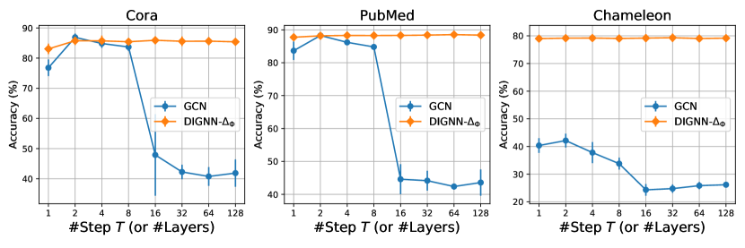
Figure 1: Over-smoothing analysis w/ #step $T$ (or #layers).

6.3 Empirical validation of theoretical results

Over-smoothing. We carry out node classification experiments on Cora, PubMed, and Chameleon datasets to show our model would not suffer from over-smoothing and performs well with large iteration steps $T$. Figure 1 illustrates that as the number of steps (or layers for GCN) increases, our model maintains good performance whilst GCN degrades catastrophically. It shows that DIGNN-$\Delta_{\Phi}$ can avoid over-smoothing for Cora, PubMed, and Chameleon datasets.

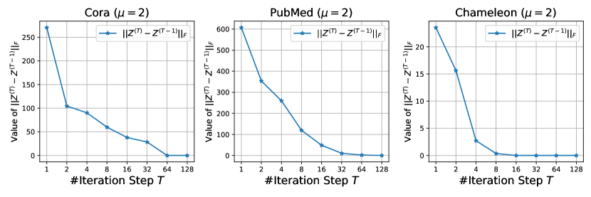
Figure 2: Convergence analysis w/ #step $T$.

Convergence analysis. We conduct experiments on Cora, PubMed, and Chameleon datasets to investigate the convergence properties of the implicit layers for DIGNN-$\Delta_{\Phi}$ concerning different iteration numbers $T$. We use $\mu=2$ and other hyperparameters from Table 5. The results of Figure 2 state as $T$ increases, the value of $\|{\mathbf{Z}}^{(T)}-{\mathbf{Z}}^{(T-1)}\|_{F}$ on three datasets quickly decreases and approaches to $0$. It validates the convergence results given in Corollary 5.3.

The impact of hyperparameter $\mu$. We study the impact of $\mu$ on the performance of DIGNN-$\Delta_{\Phi}$ for Cora and PubMed datasets. We use $T=10$ and other hyperparameters following Table 5 and fix the spectral norm of $\Theta_{\chi},\Theta_{\phi}$ at $1$ by applying spectral normalization on them. The results of PubMed in Figure 3 indicate that as $\mu$ increases from $1$ to $2$, both the term $\|{\mathbf{Z}}^{(T)}-{\mathbf{Z}}^{(T-1)}\|_{F}$ and the generalization gap $|L_{u}(f)-\widehat{L}_{m}(f)|$ decreases. Similar observation to the results of Cora. This indicates that, within a certain range, as $\mu$ increases ($\frac{\lambda_{\Phi}}{\mu}$ will decrease as $\|\Theta_{\chi}\|,\|\Theta_{\phi}\|$ are fixed), DIGNN-$\Delta_{\Phi}$ will have better convergence and generalization properties. It also validates the discussion in Remark 5.7 that fast convergence results in better generalization.

When $\mu>2$, $\|{\mathbf{Z}}^{(T)}-{\mathbf{Z}}^{(T-1)}\|_{F}$ approaches to $0$ but the generalization gap increases. It is reasonable as for $\mu>2$, DIGNN-$\Delta_{\Phi}$ already converges well and its performance becomes more influenced by other factors. As $\mu$ increases, Eq. 8 would impose more emphasis on ensuring the input feature constraints and less on feature smoothing. However, overly emphasizing the constraints, e.g., $\mu\geq 5$, could lead to overfitting in the input and output layers described in Eq. 16 in Eq. 18 respectively, which are assumed to exhibit constant Lipschitness in our theoretical analysis.

These results support our claim in Remark 5.7 that $\mu$ not only controls the trade-off between feature smoothing and input constraints in Eq. 8, but also influences the convergence and generalization properties for the model.

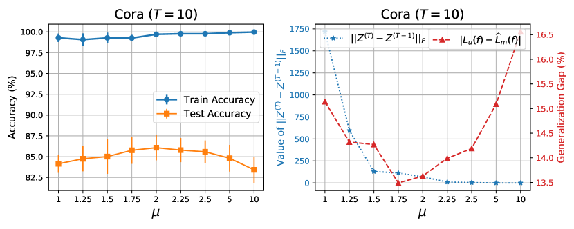
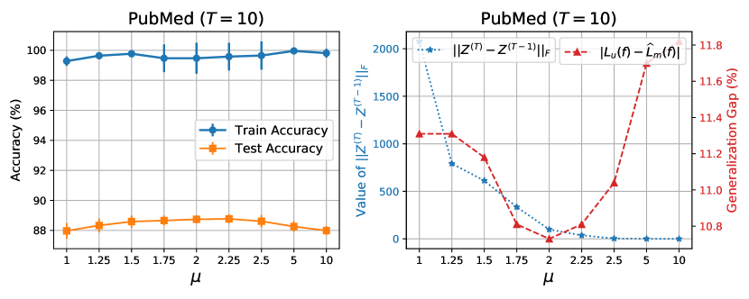
Figure 3: The impact of $\mu$ for Cora and PubMed datasets.

7 Conclusion

This paper introduces a geometric framework to equip implicit GNNs with the ability to learn the metrics of vertex and edge spaces while avoiding over-smoothing and ensuring reliable convergence and generalization properties. We further propose a new implicit GNN model based on our framework and derive new convergence and generalization results. Our model empirically works well on benchmark datasets for both node and graph classification tasks.

Appendix

.tocmtappendix mtchapternone mtappendixsubsection

Appendix A Related Work and Discussion

In this section, we discuss the related work and highlight our contributions against existing approaches. Our work generally pertains to several areas, including implicit GNNs, graph neural diffusions, Over-smoothing analysis and generalization bounds for GNNs, and graph-based semi-supervised learning.

Implicit GNNs. Instead of stacking a series of propagation layers hierarchically, implicit GNNs define their outputs as solutions to fixed-point equations, which are equivalent to running infinite-depth GNNs. As a result, implicit GNNs are able to capture long-range dependencies and benefit from the global receptive field. Moreover, by using implicit differentiation (Krantz and Parks,, 2002) for the backward pass gradient computation, implicit GNNs require only constant training memory (Bai et al.,, 2019; Ghaoui et al.,, 2019). A series of implicit GNN architectures, e.g., (Scarselli et al.,, 2009; Gu et al.,, 2020; Liu et al.,, 2021; Park et al.,, 2022; Chen et al.,, 2022; Liu et al.,, 2022), have been proposed. Probably one of the earliest implicit GNN models, proposed by (Scarselli et al.,, 2009), is based on a constrained information diffusion mechanism and it guarantees the existence of a unique stable equilibrium. The implicit layers of IGNN (Gu et al.,, 2020) and EIGNN (Liu et al.,, 2021) are developed based on the aggregation scheme of GCN (Kipf and Welling,, 2017), which corresponds to an isotropic linear diffusion operator that treats all neighbors equally and is independent of the neighbor features (Wang et al.,, 2021; Chen et al.,, 2022). CGS (Park et al.,, 2022) adopts an input-dependent learnable propagation matrix in their implicit layer which ensures guaranteed convergence and uniqueness for the fixed-point solution. However, (Oono and Suzuki, 2020a, ) shows that isotropic linear diffusion operators would lead to the over-smoothing issue. Therefore, GIND (Chen et al.,, 2022) designs a non-linear diffusion operator with anisotropic properties whose equilibrium state corresponds to a convex objective and the anisotropic property may mitigate over-smoothing. Additionally, to incorporate multiscale information on graphs, MGNNI (Liu et al.,, 2022) expands the effective range of EIGNN for capturing long-range dependencies to multiscale graph structures.

Graph neural diffusions. GNNs can be interpreted as diffusion processes on graphs. (Atwood and Towsley,, 2016; Klicpera et al., 2019b, ) design their graph convolutions based on diffusion operators and (Liao et al.,, 2019) introduces a polynomial graph filter to exploit multi-scale graph information which is closely related to diffusion maps. On the other hand, neural differential equations (Chen et al.,, 2018; Kidger,, 2022) have also been applied to design graph neural diffusion processes. Continuous depth GNNs, such as CGNN (Xhonneux et al.,, 2020), GRAND (Chamberlain et al., 2021b, ), PDE-GCN (Eliasof et al.,, 2021), have been developed based on the discretization of diffusion partial differential equations (PDEs) on graphs. (Thorpe et al.,, 2022) introduces a source term into the diffusion process of GRAND to mitigate the over-smoothing issue. (Wang et al.,, 2021) shows the equivalence between the propagation scheme of GCN and the numerical discretization of an isotropic diffusion process. Specific PDEs could be helpful to improve the capability of GNNs in capturing the graph metrics or mitigating the over-smoothing issue. For example, (Chamberlain et al., 2021a, ) develops graph diffusion equations based on the discretized Beltrami flow which facilitates feature learning, positional encoding, and graph rewiring within the diffusion process. Keriven, (2022) employs cellular sheaf theory to develop neural diffusion processes capable of handling heterophilic graphs and addressing the over-smoothing issue.

While the above implicit GNN and graph neural diffusion models have demonstrated their effectiveness in many applications, they have mainly concentrated on learning the diffusion strength without explicitly engaging in learning the metrics of vertex and edge spaces. The underlying graph metric has been shown to have a profound connection with the performance of GNNs in heterophilic settings and their over-smoothing behaviours (Bodnar et al.,, 2022). These methods may lack of sufficient adaptability in learning the graph metrics, which could potentially hinder their performance in more broad graph learning problems. On the contrary, we use three parametrized positive real-valued functions to explicitly learn the Hilbert spaces for vertices, the Hilbert space for edges, and the graph diffusion strength on each edge, respectively. Therefore, our model could have more flexibility in modeling the graph metrics.

Over-Smoothing Analysis of GNNs. Over-smoothing issues have been widely studied in deep GNN architectures. A series of works, e.g., Li et al., (2018); Zhou et al., (2021); Keriven, (2022); Zhao and Akoglu, (2020); Wang et al., (2021); Wu et al., (2023), have demonstrated that as the number of explicit GNN layers goes to infinity, the representations will converge to the same value across all nodes, which we call over-smoothing issue during training (OST). In this work, we characterize the conditions for implicit GNN layers, i.e., if the graph parameterizations are not defined as functions of the input node features, that will lead to the same OST issue. Additionally, Thorpe et al., (2022) has presented a random walk interpretation of GRAND, showing that the node features will become the same across all nodes under the GRAND-l dynamics. Another type of issue we call over-smoothing during inference (OSI). Our work shows that the same OSI issue could present in implicit GNN architectures for the task without node label constraints during the inference process, such as graph classification.

Generalization Bounds of GNNs. Numerous studies have established generalization bounds for explicit GNNs. They can categorized into the bounds derived based on Vapnik–Chervonenkis dimension (Scarselli et al.,, 2018), Rademacher complexity (Garg et al.,, 2020; Oono and Suzuki, 2020b, ; Esser et al.,, 2021; Tang and Liu,, 2023), PAC-bayesian (Liao et al.,, 2021; Ju et al.,, 2023), algorithmic stability (Verma and Zhang,, 2019; Zhou and Wang,, 2021; Cong et al.,, 2021), neural tangent kernel (Du et al.,, 2019), and many others (Yehudai et al.,, 2021; Baranwal et al.,, 2021; Li et al.,, 2022; Maskey et al.,, 2022). However, the generalization analysis for implicit GNNs is relatively overlooked and the emphasis in existing implicit GNN literature is only on ensuring convergence properties. In this work, we derive new convergence and generalization results for our implicit GNN model. Specifically, we demonstrate that with an appropriately chosen hyperparameter greater than the largest eigenvalue of the parameterized graph Laplacian, our proposed implicit graph diffusion layer is guaranteed to converge to the equilibrium. We also derive the transductive generalization bounds for our model based on the transductive Rachamecher complexity. Our theoretical results further reveal a significant link between convergence and generalization properties for implicit GNNs, indicating that superior transductive generalization ability requires fast convergence for implicit graph diffusion.

Graph-based semi-supervised learning. Graph-based semi-supervised learning algorithms usually assume that the labels of neighboring nodes in a graph are the same or consistent. Over the past few decades, numerous methods have been proposed. They generally intend to minimize a smoothness regularizer with label constraints at some vertices to ensure label consistency among neighboring nodes. Such a smoothness regularizer can be various, including graph Laplacian regularization (Zhu et al.,, 2003; Smola and Kondor,, 2003; Zhou et al.,, 2004; Belkin et al.,, 2004; Zhou and Schölkopf,, 2005; Nadler et al.,, 2009; Slepcev and Thorpe,, 2017; Weihs and Thorpe,, 2023), Tikhonov regularization (Belkin et al.,, 2004), manifold regularizations (Belkin et al.,, 2006; Niyogi,, 2013). We refer to (Zhu,, 2005; van Engelen and Hoos,, 2020) for a more comprehensive review of graph-based semi-supervised learning. These methods are developed based on non-parameterized graph Laplacians whose vertex and edge spaces are fixed and independent of the node features. As we characterized in Corollary 4.2, this could lead to over-smoothing during training (OST), i.e., changing the node features will not affect the output node representations during training. Moreover, when it comes to graph classification or graph regression problems that do not have label constraints during the inference process, Lemma 4.1 shows that their output may converge to a constant function over all nodes regardless of the input features, a problem we call over-smoothing during inference (OSI). Grounding on the theoretical justifications, our derived model can overcome these two types of over-smoothing issues.

Limitations. One of the main limitations of our work is that our theoretical analysis and methodology have focused on linear graph neural diffusion operators. However, the theoretical foundation for non-linear dynamic systems remains an important impediment to the entire field of machine learning. Nonetheless, our work has provided some valuable insights into the interplay between implicit GNNs, differential geometry, and semi-supervised learning. There are still numerous unexplored insights to be discovered and we look forward to seeing further cross-fertilization between machine learning and algebraic topology in the future.

Appendix B Theorems and Proofs

B.1 Theorems and proofs in Section 3

B.1.1 Proof of Lemma 3.7

Lemma 3.7. Given an undirected graph ${\mathcal{G}}=({\mathcal{V}},{\mathcal{E}})$ and a function $g:{\mathcal{E}}\mapsto\mathbb{R}$, the parameterized graph divergence $\mathrm{div}:{\mathcal{H}}({\mathcal{E}},\phi)\mapsto{\mathcal{H}}({\mathcal{V}},\chi)$ is explicitly given by

$$(\mathrm{div}g)(i)=\frac{1}{2\chi(i)}\sum_{j=1}^{n}\varphi([i,j])\phi([i,j])\left(g([i,j])-g([j,i])\right).$$

Proof.

For any $k=1,2,\dots,n$, using the indicator function $f(i)={\mathbb{I}}_{i=k}$, where

$${\mathbb{I}}_{i=k}=\begin{cases}1&\text{ if }i=k,\\ 0&\text{ if }i\neq k.\end{cases}$$

By the definition of the inner product on the function space on the edges, we have

$$\langle\nabla{\mathbb{I}}_{\cdot=k},g\rangle_{\mathcal{E}}={} \frac{1}{2}\sum_{i=1}^{n}\sum_{j=1}^{n}(\nabla{\mathbb{I}}_{\cdot=k})([i,j])g([i,j])\phi([i,j])$$

$$={} \frac{1}{2}\sum_{i=1}^{n}\sum_{j=1}^{n}\varphi([i,j])({\mathbb{I}}_{j=k}-{\mathbb{I}}_{i=k})g([i,j])\phi([i,j])$$

$$={} \frac{1}{2}\left(\sum_{i=1}^{n}\sum_{j=1}^{n}\varphi([i,j]){\mathbb{I}}_{j=k}g([i,j])\phi([i,j])-\sum_{i=1}^{n}\sum_{j=1}^{n}\varphi([i,j]){\mathbb{I}}_{i=k})g([i,j])\phi([i,j])\right)$$

$$={} \frac{1}{2}\left(\sum_{i=1}^{n}\varphi([i,k])g([i,k])\phi([i,k])-\sum_{j=1}^{n}\varphi([k,j])g([k,j])\phi([k,j])\right)$$

$$={} \frac{1}{2}\left(\sum_{j=1}^{n}\varphi([j,k])g([j,k])\phi([j,k])-\sum_{j=1}^{n}\varphi([k,j])g([k,j])\phi([k,j])\right) i j$$ (Replace by for the first term)

$$={} \frac{1}{2}\left(\sum_{j=1}^{n}\varphi([k,j])\phi([k,j])g([j,k])-\sum_{j=1}^{n}\varphi([k,j])\phi([k,j])g([k,j])\right) [k,j]=[j,k]$$ ( for undirected graphs)

$$={} \frac{1}{2}\sum_{j=1}^{n}\varphi([k,j])\phi([k,j])\left(g([j,k])-g([k,j])\right).$$

Note that

$$\langle{\mathbb{I}}_{\cdot=k},\mathrm{div}g\rangle_{\mathcal{V}}={} \sum_{i=1}^{n}({\mathbb{I}}_{i=k})(\mathrm{div}g)(i)\chi(i)$$

$$={} (\mathrm{div}g)(k)\chi(k).$$

Note also that

$$\langle{\mathbb{I}}_{\cdot=k},-\mathrm{div}g\rangle_{\mathcal{V}}=\langle\nabla{\mathbb{I}}_{\cdot=k},g\rangle_{\mathcal{E}}$$

$$\Longrightarrow{} (\mathrm{div}g)(k)\chi(k)=-\frac{1}{2}\sum_{j=1}^{n}\varphi([k,j])\phi([k,j])\left(g([j,k])-g([k,j])\right)$$

$$\Longrightarrow{} (\mathrm{div}g)(k)=\frac{1}{2\chi(k)}\sum_{j=1}^{n}\varphi([k,j])\phi([k,j])\left(g([k,j])-g([j,k])\right).$$

∎

B.1.2 Proof of Lemma 3.9

Lemma 3.9. Given an undirected graph ${\mathcal{G}}=({\mathcal{V}},{\mathcal{E}})$ and a function $f:{\mathcal{V}}\mapsto\mathbb{R}$, we have for all $i\in{\mathcal{V}}$,

$$(\Delta_{\Phi}f)(i)=\frac{1}{\chi(i)}\sum_{j=1}^{n}\varphi([i,j])^{2}\phi([i,j])\left(f(i)-f(j)\right).$$

Proof.

For all $i\in{\mathcal{V}}$,

$$(\Delta_{\Phi}f)(i)={} (-\mathrm{div}\nabla f)(i)$$

$$={} -\frac{1}{2\chi(i)}\sum_{j=1}^{n}\varphi([i,j])\phi([i,j])\left(\nabla f([i,j])-\nabla f([j,i])\right)$$

$$={} \frac{1}{2\chi(i)}\sum_{j=1}^{n}\varphi([i,j])\phi([i,j])\left(\nabla f([j,i])-\nabla f([i,j])\right)$$

$$={} \frac{1}{2\chi(i)}\sum_{j=1}^{n}\varphi([i,j])\phi([i,j])\left(\varphi([j,i])\left(f(i)-f(j)\right)-\varphi([i,j])\left(f(j)-f(i)\right)\right)$$

$$={} \frac{1}{2\chi(i)}\sum_{j=1}^{n}\varphi([i,j])\phi([i,j])\left(\varphi([i,j])\left(f(i)-f(j)\right)-\varphi([i,j])\left(f(j)-f(i)\right)\right) [j,i]=[i,j]$$ ()

$$={} \frac{1}{\chi(i)}\sum_{j=1}^{n}\varphi([i,j])^{2}\phi([i,j])\left(f(i)-f(j)\right).$$

∎

B.1.3 Proposition B.1 and proof

Proposition B.1.

For any graph ${\mathcal{G}}=({\mathcal{V}},{\mathcal{E}})$ and any positive real-valued functions $\chi:{\mathcal{V}}\mapsto\mathbb{R}_{+},\phi:{\mathcal{E}}\mapsto\mathbb{R}^{+},\varphi:{\mathcal{E}}\mapsto\mathbb{R}_{+}^{*}$, the parameterized graph Laplacian $\Delta_{\Phi}:{\mathcal{H}}({\mathcal{V}},\chi)\mapsto{\mathcal{H}}({\mathcal{V}},\chi)$ is self-adjoint and positive semi-definite.

Proof.

By the definition of parameterized graph Laplacian,

$$\langle f,\Delta_{\Phi}g\rangle_{\mathcal{V}}={} \langle f,-\mathrm{div}\nabla g\rangle_{\mathcal{V}}$$

$$={} \langle\nabla f,\nabla g\rangle_{\mathcal{E}}$$

$$={} \langle-\mathrm{div}\nabla f,g\rangle_{\mathcal{V}}$$

$$={} \langle\Delta_{\Phi}f,g\rangle_{\mathcal{V}},$$

which indicates the self-adjoint and

$$\langle f,\Delta_{\Phi}f\rangle_{\mathcal{V}}={} \langle f,-\mathrm{div}\nabla f\rangle_{\mathcal{V}}$$

$$={} \langle\nabla f,\nabla f\rangle_{\mathcal{E}}\geq 0,$$

which indicates the positive semi-definite. ∎

B.1.4 Lemma B.2 and proof

Lemma B.2.

Given a vector function $f:{\mathcal{V}}\mapsto\mathbb{R}^{c}$, for any positive real-valued functions $\chi:{\mathcal{V}}\mapsto\mathbb{R}_{+},\phi:{\mathcal{E}}\mapsto\mathbb{R}_{+},\varphi:{\mathcal{E}}\mapsto\mathbb{R}_{+}^{*}$, we have

$$\left.\frac{{\mathrm{d}}{\mathcal{S}}(f)}{{\mathrm{d}}f}\right|_{i}=2\chi(i)(\Delta_{\Phi}f)(i).$$ (23)

Proof.

$$\left.\frac{{\mathrm{d}}{\mathcal{S}}(f)}{{\mathrm{d}}f}\right|_{i}={} \left.\frac{{\mathrm{d}}}{{\mathrm{d}}f}\frac{1}{2}\sum_{i=1}^{n}\sum_{j=1}^{n}\varphi([i,j])^{2}\phi([i,j])\left\|f(j)-f(i)\right\|^{2}\right|_{i}$$

$$={} \sum_{i=1}^{n}\varphi([i,j])^{2}\phi([i,j])(f(j)-f(i))+\sum_{j=1}^{n}\varphi([i,j])^{2}\phi([i,j])(f(i)-f(j))$$

$$={} \sum_{j=1}^{n}\varphi([j,i])^{2}\phi([j,i])(f(i)-f(j))+\sum_{j=1}^{n}\varphi([i,j])^{2}\phi([i,j])(f(i)-f(j)) i j$$ (exchange and for the first term)

$$={} 2\sum_{j=1}^{n}\varphi([i,j])^{2}\phi([i,j])(f(i)-f(j)) [j,i]=[i,j]$$ ()

$$={} 2\chi(i)(\Delta_{\Phi}f)(i).$$

∎

B.2 Theorems and proofs in Section 4

B.2.1 Proof of Lemma 4.1

Lemma 4.1 (Convergence and Uniqueness Analysis). Let $\gamma_{\text{max}}$ be the largest singular value of ${\mathbf{C}}$. The fixed-point equilibrium equation (Eq. 9) has a unique solution if $\gamma_{\text{max}}<1$. We can iterate the equation:

$$f^{(t+1)}={\mathbf{Y}}^{\prime}+{\mathbf{C}}f^{(t)},\quad t=0,1,\dots.$$

to obtain the optimal solution $f^{\star}=\lim_{t\rightarrow\infty}f^{(t)}$ which is independent of the initial state $f^{(0)}$.

Proof.

For $t\geq 1$ and the sequence $f^{(0)},f^{(1)},\dots$ generated by $f^{(t+1)}={\mathbf{Y}}^{\prime}+{\mathbf{C}}f^{(t)}$,

$$\|f^{(t+1)}-f^{(t)}\|\leq{} \left\|{\mathbf{Y}}^{\prime}+{\mathbf{C}}f^{(t)}-{\mathbf{Y}}^{\prime}-{\mathbf{C}}f^{(t-1)}\right\|$$

$$={} \left\|({\mathbf{C}}f^{(t)}-{\mathbf{C}}f^{(t-1)}\right\|$$

$$\leq{} \|{\mathbf{C}}\|\|f^{(t)}-f^{(t-1)}\|.$$

For $n>m\geq 1$, the following inequality holds,

$$\|f^{(n)}-f^{(m)}\|={} \|f^{(n)}-f^{(n-1)}+f^{(n-1)}-\dots+f^{(m+1)}-f^{(m)}\|$$

$$\leq{} \sum_{t=m}^{n-1}\|f^{(t+1)}-f^{(t)}\|$$

$$\leq{} \sum_{t=m}^{n-1}\|{\mathbf{C}}\|^{t-m}\|f^{(m+1)}-f^{(m)}\|$$

$$\leq{} \sum_{t=m}^{n-1}\|{\mathbf{C}}\|^{t-m}\|{\mathbf{C}}\|^{m}\|f^{(1)}-f^{(0)}\|$$

$$={} \|{\mathbf{C}}\|^{m}\sum_{t=0}^{n-m-1}\|{\mathbf{C}}\|^{t}\|f^{(1)}-f^{(0)}\|$$

$$\leq{} \|{\mathbf{C}}\|^{m}\sum_{t=0}^{\infty}\|{\mathbf{C}}\|^{t}\|f^{(1)}-f^{(0)}\|$$

$$={} \|{\mathbf{C}}\|^{m}(1-\|{\mathbf{C}}\|)^{-1}\|f^{(1)}-f^{(0)}\|.$$

If $\gamma_{\text{max}}<1$, we have $\|{\mathbf{C}}\|=\gamma_{\text{max}}<1$, which implies that $\|{\mathbf{C}}\|^{m}(1-\|{\mathbf{C}}\|)^{-1}\|f^{(1)}-f^{(0)}\|\geq 0$, then the inequality $\|f^{(n)}-f^{(m)}\|\leq(\|{\mathbf{C}}\|)^{m}(1-\|{\mathbf{C}}\|)^{-1}\|f^{(1)}-f^{(0)}\|$ is well-posed. Note also that when $\|{\mathbf{C}}\|<1$, we have $\lim_{t\rightarrow\infty}(\|{\mathbf{C}}\|)^{t}=0$ and $\lim_{t\rightarrow\infty}(\|{\mathbf{C}}\|)^{t}(1-\|{\mathbf{C}}\|)^{-1}=0$. Then the sequence $f^{(0)},f^{(1)},f^{(2)},\dots$ is a Cauchy sequence because

$$0\leq\lim_{m\rightarrow\infty}\|f^{(n)}-f^{(m)}\|\leq\lim_{m\rightarrow\infty}(\|{\mathbf{C}}\|)^{m}(1-\|{\mathbf{C}}\|)^{-1}\|f^{(1)}-f^{(0)}\|=0.$$

Thus the sequence converges to some solution of $f^{\star}={\mathbf{Y}}^{\prime}+{\mathbf{C}}f^{\star}$.

To prove the uniqueness, suppose that both $f^{(a)}$ and $f^{(b)}$ satisfy $f={\mathbf{Y}}^{\prime}+{\mathbf{C}}f$, i.e., $f^{(a)}={\mathbf{Y}}^{\prime}+{\mathbf{C}}f^{(a)}$ and $f^{(b)}={\mathbf{Y}}^{\prime}+{\mathbf{C}}f^{(b)}$. Then we have

$$0\leq{} \|f^{(a)}-f^{(b)}\|$$

$$={} \left\|{\mathbf{Y}}^{\prime}+{\mathbf{C}}f^{(a)}-{\mathbf{Y}}^{\prime}(i)-{\mathbf{C}}f^{(b)}\right\|$$

$$={} \left\|{\mathbf{C}}f^{(a)}-{\mathbf{C}}f^{(b)}\right\|$$

$$\leq{} \|{\mathbf{C}}\|\|f^{(a)}-f^{(b)}\|$$

$$={} \|{\mathbf{C}}\|\left\|{\mathbf{Y}}^{\prime}+{\mathbf{C}}f^{(a)}-{\mathbf{Y}}^{\prime}-{\mathbf{C}}f^{(b)}\right\|$$

$$\leq{} \lim_{t\rightarrow\infty}\left(\|{\mathbf{C}}\|\right)^{t}\|f^{(a)}-f^{(b)}\|=0, \lim_{t\rightarrow\infty}\left(\|{\mathbf{C}}\|\right)^{t}=0 \gamma_{\text{max}}<1$$ ( when )

which indicates that $f^{(a)}=f^{(b)}$ and there exists unique solution to $f={\mathbf{Y}}^{\prime}+{\mathbf{C}}f$ if $\gamma_{\text{max}}<1$. ∎

B.2.2 Proof of Corollary 4.2

Corollary 4.2 (Over-Smoothing during Training (OST) Condition). Assume that the initial state $f^{(0)}$ at node $i$ is initialized as a function of ${\mathbf{x}}_{i}$. Assume further that $\chi,\phi,\varphi$ are not functions of ${\mathbf{x}}_{i}$, e.g., $\Delta$ is the unnormalized Laplacian or random walk Laplacian. Let $\gamma_{\text{max}}$ be the largest singular value of ${\mathbf{C}}$. Then, if $\gamma_{\text{max}}<1$, the equilibrium of the fixed point equation Eq. 9 is independent of the node features ${\mathbf{x}}_{i}$, i.e. the same equilibrium solution is obtained even if the node features ${\mathbf{x}}_{i}$ are changed.

Proof.

When $\gamma_{\text{max}}<1$, by Lemma 4.1 we know that the fixed-point equation Eq. 9 has a unique equilibrium. Since $\chi,\varphi$, and $\varphi$ are not functions of ${\mathbf{x}}_{i}$, $\Delta$ is independent of the node features ${\mathbf{x}}_{i},\forall i\in{\mathcal{V}}$. Therefore, $\gamma_{\text{max}}$ is independent of the node features, which indicates that the uniqueness condition of the equilibrium is also independent of the node features. ∎

B.2.3 Proof of Lemma 4.3

Lemma 4.3 (Over-Smoothing during Inference (OSI) Condition). When ${\mathcal{I}}=\emptyset$, i.e., there is no constrained nodes in Eq. 8, we have ${\mathbf{C}}={\mathbf{P}}$ and ${\mathbf{y}}^{\prime}(i)=\mathbf{0},\forall i\in{\mathcal{V}}$. ${\mathbf{P}}$ is a Markov matrix and the solution of Eq. 8 satisfies $f={\mathbf{P}}f$. If the graph ${\mathcal{G}}$ is connected and non-bipartite, i,e., the Markov chain corresponding to ${\mathbf{P}}$ is irreducible and aperiodic, the equilibrium $f^{\star}(i)$ for all nodes are identical and not unique, i.e., $f^{\star}(i)={\mathbf{v}},\forall i\in{\mathcal{V}}$, where ${\mathbf{v}}$ is any vector in $\mathbb{R}^{c}$ and is independent of the labels. Iterating $f^{(t+1)}={\mathbf{P}}f^{(t)},t=0,1,\dots,$ with initial state $f^{(0)}\in\mathbb{R}^{n\times c}$ will converge to

$$f^{\star}(i)=(\lim_{t\rightarrow\infty}{\mathbf{P}}^{t}f^{(0)})(i)=({\bm{\pi}}f^{(0)})^{\top},\quad\forall i\in{\mathcal{V}},$$

where $\bm{\pi}=(\widehat{{D}}_{1}/\sum_{j}\widehat{{D}}_{j},\dots,\widehat{{D}}_{n}/\sum_{j}\widehat{{D}}_{j})\in\mathbb{R}^{1\times n}$ is the stationary distribution of ${\mathbf{P}}$.

Proof.

If the graph is connected and non-bipartite, the Markov chain corresponding to ${\mathbf{P}}$ is irreducible and aperiodic. Then by the Fundamental Theorem of Markov chains (Meyn and Tweedie,, 2012), ${\mathbf{P}}$ has a unique stationary distribution. Let ${\bm{\pi}}=(\pi_{1},\dots,\pi_{n})\in\mathbb{R}^{1\times n}$ be the stationary distribution of ${\mathbf{P}}$, then

$${\bm{\pi}}={\bm{\pi}}{\mathbf{P}}.$$

${\bm{\pi}}$ is given by $(\widehat{{D}}_{1}/\sum_{j}\widehat{{D}}_{j},\dots,\widehat{{D}}_{n}/\sum_{j}\widehat{{D}}_{j})$, which can be easily verified by

$$\sum_{i=1}^{n}\pi_{i}{P}_{i,j}={} \sum_{i=1}^{n}\frac{\widehat{{D}}_{i}}{\sum_{k=1}^{n}\widehat{{D}}_{k}}\frac{\varphi([i,j])^{2}\phi([i,j])}{\widehat{{D}}_{i}}$$

$$={} \frac{\sum_{i=1}^{n}\varphi([i,j])^{2}\phi([i,j])}{\sum_{k=1}^{n}\widehat{{D}}_{k}}$$

$$={} \frac{\widehat{{D}}_{j}}{\sum_{k=1}^{n}\widehat{{D}}_{k}}$$

$$={} \pi_{j}.$$

By the Fundamental Theorem of Markov chains, we have

$$\lim_{t\rightarrow\infty}({\mathbf{P}}^{t})_{i,j}=\pi_{j},\quad\text{for all }i,j\in{\mathcal{V}},$$

which indicates that as $t$ goes to infinity, all row vectors in ${\mathbf{P}}^{t}$ are identical and is the stationary vector ${\bm{\pi}}$ of ${\mathbf{P}}$, i.e., $\lim_{t\rightarrow\infty}{\mathbf{P}}^{t}=({\bm{\pi}}^{\top},\dots,{\bm{\pi}}^{\top})^{\top}$. Denote $f^{\star}=(f^{\star}(1),\dots,f^{\star}(n))^{\top}\in\mathbb{R}^{n\times c}$, then

$$f^{\star}(i)=({\mathbf{P}}f^{\star})(i)=({\mathbf{P}}{\mathbf{P}}f^{\star})(i)=(\lim_{t\rightarrow\infty}{\mathbf{P}}^{t}f^{\star})(i)=(({\bm{\pi}}^{\top},\dots,{\bm{\pi}}^{\top})^{\top}f)(i)=({\bm{\pi}}f^{\star})^{\top},\quad\forall i\in{\mathcal{V}}.$$

which indicates that the equilibrium of all nodes are identical. $({\bm{\pi}}f)^{\top}$ can be any vector in $\mathbb{R}^{c}$, therefore any vector ${\mathbf{v}}\in\mathbb{R}^{c}$, $f^{\star}=({\mathbf{v}},\dots,{\mathbf{v}})^{\top}\in\mathbb{R}^{n\times d}$ is an equilibrium of the fixed-point equation $f={\mathbf{P}}f$. Hence, the equilibrium is a constant function over all nodes.

Moreover, iterating $f^{(t+1)}={\mathbf{P}}f^{(t)}$ with an initial state $f^{(0)}$ with converge to

$$\lim_{t\rightarrow\infty}f^{(t+1)}(i)=(\lim_{t\rightarrow\infty}{\mathbf{P}}^{t}f^{(0)})(i)=(({\bm{\pi}}^{\top},\dots,{\bm{\pi}}^{\top})^{\top}f^{(0)})(i)=({\bm{\pi}}f^{(0)})^{\top},\quad\text{for all }i\in{\mathcal{V}},$$

which is an equilibrium of the fixed-point equation $f={\mathbf{P}}f$. ∎

B.3 Theorems and proofs in Section 5

B.3.1 Proof of Theorem 5.1

Theorem 5.1 (Spectral Range of $\Delta_{\Phi}$). Let $\Delta_{\Phi}$ be the graph neural Laplacian and $\chi,\phi,\varphi$ are given by Eq. 12, 13 and 14 respectively, $\lambda_{\Phi}$ be an eigenvalue associated with the eigenvector ${\mathbf{u}}$ of $\Delta_{\Phi}$. Suppose Assumptions 1, 2 and 3 hold, then

$$0\leq\lambda_{\Phi}\leq 2c_{\phi}^{2}c_{\chi}c_{X}\cosh(c_{\chi}c_{X}).$$

Proof.

Note that by Proposition B.1 the graph neural Laplacian is positive semi-definite and therefore we have $\lambda_{\Phi}\geq 0$. On the other hand, by the definition of parameterized graph Laplacian, we have for all $i=1,2,\dots,n$,

$$(\Delta_{\Phi}{\mathbf{u}})_{i}=\frac{1}{\chi(i)}\sum_{j=1}^{n}\varphi([i,j])^{2}\phi([i,j])({u}_{i}-{u}_{j})=\lambda_{\Phi}{u}_{i}.$$

Then we have for all $i=1,\dots,n$,

$$\lambda_{\Phi}={} \frac{1}{{u}_{i}}\sum_{j=1}^{n}\frac{\varphi([i,j])^{2}\phi([i,j])}{\chi(i)}({u}_{i}-{u}_{j})$$

$$={} \sum_{j=1}^{n}\frac{\varphi([i,j])^{2}\phi([i,j])}{\chi(i)}(1-\frac{{u}_{j}}{{u}_{i}})$$

$$\leq{} \sum_{j=1}^{n}\frac{\varphi([i,j])^{2}\phi([i,j])}{\chi(i)}\left(1+\left|\frac{{u}_{j}}{{u}_{i}}\right|\right)$$

$$={} \sum_{j=1}^{n}\frac{{A}_{i,j}}{{D}_{i}}\frac{\tanh((\|\Theta_{\varphi}({\mathbf{x}}_{i}-{\mathbf{x}}_{j})\|+\epsilon)^{-1})\tanh(|(\Theta_{\phi}\Theta_{\chi}{\mathbf{x}}_{i})^{\top}(\Theta_{\phi}\Theta_{\chi}{\mathbf{x}}_{j})|)}{\tanh(\|\Theta_{\chi}{\mathbf{x}}_{i}\|)}\left(1+\left|\frac{{u}_{j}}{{u}_{i}}\right|\right)$$

$$\leq{} \sum_{j=1}^{n}\frac{{A}_{i,j}}{{D}_{i}}\frac{\tanh(|(\Theta_{\phi}\Theta_{\chi}{\mathbf{x}}_{i})^{\top}(\Theta_{\phi}\Theta_{\chi}{\mathbf{x}}_{j})|)}{\tanh(\|\Theta_{\chi}{\mathbf{x}}_{i}\|)}\left(1+\left|\frac{{u}_{j}}{{u}_{i}}\right|\right) \tanh(a)\leq 1,\forall a\in\mathbb{R}$$ ()

$$\leq{} \sum_{j=1}^{n}\frac{{A}_{i,j}}{{D}_{i}}\frac{|(\Theta_{\phi}\Theta_{\chi}{\mathbf{x}}_{i})^{\top}(\Theta_{\phi}\Theta_{\chi}{\mathbf{x}}_{j})|}{\tanh(\|\Theta_{\chi}{\mathbf{x}}_{i}\|)}\left(1+\left|\frac{{u}_{j}}{{u}_{i}}\right|\right) \tanh(a)\leq a,\forall a\in\mathbb{R}$$ ()

$$={} \sum_{j=1}^{n}\frac{{A}_{i,j}}{{D}_{i}}\frac{|(\Theta_{\phi}\Theta_{\chi}{\mathbf{x}}_{i})^{\top}(\Theta_{\phi}\Theta_{\chi}{\mathbf{x}}_{j})|\cosh(\|\Theta_{\chi}{\mathbf{x}}_{i}\|)}{\sinh(\|\Theta_{\chi}{\mathbf{x}}_{i}\|)}\left(1+\left|\frac{{u}_{j}}{{u}_{i}}\right|\right)$$

$$\leq{} \sum_{j=1}^{n}\frac{{A}_{i,j}}{{D}_{i}}\frac{\|\Theta_{\phi}\|\|\Theta_{\chi}{\mathbf{x}}_{i}\|\|\Theta_{\phi}\Theta_{\chi}{\mathbf{x}}_{j}\|\cosh(\|\Theta_{\chi}{\mathbf{x}}_{i}\|)}{\sinh(\|\Theta_{\chi}{\mathbf{x}}_{i}\|)}\left(1+\left|\frac{{u}_{j}}{{u}_{i}}\right|\right)$$

$$\leq{} \sum_{j=1}^{n}\frac{{A}_{i,j}}{{D}_{i}}\|\Theta_{\phi}\|\|\Theta_{\phi}\Theta_{\chi}{\mathbf{x}}_{j}\|\cosh(\|\Theta_{\chi}{\mathbf{x}}_{i}\|)\left(1+\left|\frac{{u}_{j}}{{u}_{i}}\right|\right) \frac{a}{\sinh(a)}\leq 1,\forall a\in\mathbb{R}$$ ()

$$\leq{} \sum_{j=1}^{n}\frac{{A}_{i,j}}{{D}_{i}}\|\Theta_{\phi}\|^{2}\|\Theta_{\chi}\|\|{\mathbf{x}}_{j}\|\cosh(\|\Theta_{\chi}\|\|{\mathbf{x}}_{i}\|)\left(1+\left|\frac{{u}_{j}}{{u}_{i}}\right|\right)$$

$$\leq{} c_{\phi}^{2}c_{\chi}c_{X}\cosh(c_{\chi}c_{X})\left(\sum_{j=1}^{n}\frac{{A}_{i,j}}{{D}_{i}}\left(1+\left|\frac{{u}_{j}}{{u}_{i}}\right|\right)\right).$$

Since the above inequality holds for all $i=1,\dots,n$, let $k=\operatorname*{arg\,max}_{i}(\{|{u}_{i}|\}_{i=1,2,\dots,n})$, we have

$$\lambda_{\Phi}\leq{} c_{\phi}^{2}c_{\chi}c_{X}\cosh(c_{\chi}c_{X})\left(\sum_{j=1}^{n}\frac{{A}_{k,j}}{{D}_{k}}\left(1+\left|\frac{{u}_{j}}{{u}_{k}}\right|\right)\right)$$

$$\leq{} c_{\phi}^{2}c_{\chi}c_{X}\cosh(c_{\chi}c_{X})\left(\sum_{j=1}^{n}\frac{{A}_{k,j}}{{D}_{k}}\left(1+1\right)\right)$$

$$={} 2c_{\phi}^{2}c_{\chi}c_{X}\cosh(c_{\chi}c_{X}).$$

∎

B.3.2 Proof of Corollary 5.3

Corollary 5.3 (Tractable Well-Posedness Condition and Convergence Rate). Given an undirected graph ${\mathcal{G}}=({\mathcal{V}},{\mathcal{E}},{\mathbf{A}})$ with node embeddings $\widetilde{{\mathbf{X}}}:=(\widetilde{{\mathbf{x}}}_{1},\dots,\widetilde{{\mathbf{x}}}_{n})^{\top}\in\mathbb{R}^{n\times d}$, Let $\lambda_{\text{max}}$ be the largest eigenvalues of the matrix $\Delta$. Suppose that Assumption 1 holds, then, the fixed-point equilibrium equation ${\mathbf{Z}}=\widetilde{{\mathbf{X}}}-\frac{1}{\mu}\Delta{\mathbf{Z}}$ has a unique solution if $\mu>\lambda_{\text{max}}$. The solution can be obtained by iterating:

$${\mathbf{Z}}^{(t+1)}=\widetilde{{\mathbf{X}}}-\frac{1}{\mu}\Delta{\mathbf{Z}}^{(t)},\text{ with }{\mathbf{Z}}^{(0)}=\mathbf{0},t=0,1,\dots.$$

Therefore, ${\mathbf{Z}}^{\star}=\lim_{t\rightarrow\infty}{\mathbf{Z}}^{(t)}$. Suppose that $\|{\mathbf{Z}}^{\star}\|\leq c_{Z}\in\mathbb{R}_{+}^{*}$, then $\forall t\geq 1$, $\|{\mathbf{Z}}^{(t)}-{\mathbf{Z}}^{\star}\|\leq c_{Z}\left(\lambda_{\text{max}}/\mu\right)^{t}$. Specifically,

1. If $\Delta$ is the random walk Laplacian, i.e., $\Delta\equiv\Delta^{\text{(rw)}}$, $\mu>2$ and $\|{\mathbf{Z}}^{(t)}-{\mathbf{Z}}^{\star}\|\leq c_{Z}\left(2/\mu\right)^{t}$;

2. If $\Delta$ is learnable and $\Delta\equiv\Delta_{\Phi}$, suppose further that Assumptions 2 and 3 hold, then we have $\mu>2c_{\phi}^{2}c_{\chi}c_{X}\cosh(c_{\chi}c_{X})$ and $\|{\mathbf{Z}}^{(t)}-{\mathbf{Z}}^{\star}\|\leq c_{Z}(2c_{\phi}^{2}c_{\chi}c_{X}\cosh(c_{\chi}c_{X})/\mu)^{t}$.

Proof.

The fixed-point equilibrium equation ${\mathbf{Z}}=\widetilde{{\mathbf{X}}}-\frac{1}{\mu}\Delta{\mathbf{Z}}$ is a case of $f={\mathbf{Y}}^{\prime}+{\mathbf{C}}f$ when ${\mathcal{I}}\equiv{\mathcal{V}}$. Then we have ${\mathbf{C}}=-\frac{1}{\mu}\Delta$. By Proposition B.1, $\Delta$ is positive semi-definite. Therefore, the largest singular value of $\Delta$ is its largest eigenvalue. Then we have

$$\|{\mathbf{C}}\|=\|\frac{1}{\mu}\Delta\|=\frac{1}{\mu}\|\Delta\|=\frac{1}{\mu}\max_{i}|\lambda_{i}|=\frac{1}{\mu}\lambda_{\text{max}},$$

which indicates that $\gamma=\frac{1}{\mu}\lambda_{\text{max}}$. By Lemma 4.1, we have if $\frac{1}{\mu}\lambda_{\text{max}}<1$, i.e., $\mu>\lambda_{\text{max}}$, the fixed-point equilibrium equation has a unique solution and iterating Eq. 19 will convergence to the solution, i.e., ${\mathbf{Z}}^{\star}=\lim_{t\rightarrow\infty}{\mathbf{Z}}^{(t)}$. Moreover, for $t\geq 1$,

$$\|{\mathbf{Z}}^{(t)}-{\mathbf{Z}}^{\star}\|={} \|\widetilde{{\mathbf{X}}}-\frac{1}{\mu}\Delta{\mathbf{Z}}^{(t-1)}-\widetilde{{\mathbf{X}}}+\frac{1}{\mu}\Delta{\mathbf{Z}}^{\star}\|$$

$$={} \frac{1}{\mu}\|\Delta({\mathbf{Z}}^{(t-1)}-{\mathbf{Z}}^{\star})\|$$

$$\leq{} \frac{1}{\mu}\|\Delta\|\|{\mathbf{Z}}^{(t-1)}-{\mathbf{Z}}^{\star}\|$$

$$\leq{} \left(\frac{1}{\mu}\|\Delta\|\right)^{t}\|{\mathbf{Z}}^{(0)}-{\mathbf{Z}}^{\star}\|$$

$$={} \left(\frac{\lambda_{\text{max}}}{\mu}\right)^{t}\|{\mathbf{Z}}^{\star}\|$$

$$\leq{} c_{Z}\left(\frac{\lambda_{\text{max}}}{\mu}\right)^{t}.$$

1. When $\Delta$ is fixed and $\Delta\equiv\Delta^{\text{(rw)}}$. The largest eigenvalue of the random walk matrix $\lambda_{\text{max}}=2$. Therefore, we have $\mu>2$ to ensure the uniqueness of the fixed-point equation and the convergence of Eq. 19.

2. When $\Delta$ is parameterized and $\Delta\equiv\Delta_{\Phi}$. With Assumptions 2 and 3, $\|\widetilde{{\mathbf{x}}}_{i}\|\leq c_{X},\forall i\in{\mathcal{V}},\|\Theta_{\chi}\|\leq c_{\chi},\|\Theta_{\phi}\|\leq c_{\phi}$, the largest eigenvalue of $\Delta_{\Phi}$ is upper-bounded by $\lambda_{\text{max}}\leq 2c_{\phi}^{2}c_{\chi}c_{X}\cosh(c_{\chi}c_{X})$ by Theorem 5.1. Therefore, to ensure the uniqueness of the fixed-point equation and the convergence of Eq. 19 we need $2c_{\phi}^{2}c_{\chi}c_{X}\cosh(c_{\chi}c_{X})<\mu$. ∎

B.3.3 Proof of Theorem 5.6

Transductive learning on graphs. Given an undirected graph ${\mathcal{G}}=({\mathcal{V}},{\mathcal{E}},{\mathbf{A}})$ with node features and labels $\{({\mathbf{x}}_{i},y_{i})\}_{i=1}^{m+u}$ where $m+u=n$. Without loss of generality, let $\{y_{i}\}_{i=1}^{m}$ be the selected node labels, we aim to predict the labels of all nodes by a learner (model) trained on the graph ${\mathcal{G}}$ with $\{{\mathbf{x}}_{i}\}_{i=1}^{m+u}\cup\{y_{i}\}_{i=1}^{m}$. For any $f\in{\mathcal{H}}$, the training and test error is defined as:

$$\widehat{L}_{m}(f):={} \frac{1}{m}\sum_{i=1}^{m}\ell(f({\mathbf{x}}_{i}),y_{i}),$$

$$L_{u}(f):={} \frac{1}{u}\sum_{i=m+1}^{m+u}\ell(f({\mathbf{x}}_{i}),y_{i})$$

respectively, where $\ell:{\mathcal{H}}\times{\mathcal{X}}\times{\mathcal{Y}}\mapsto\mathbb{R}_{+}$ is the loss function. We are interested in the transductive generalization gap of $f$ which is defined as $|\widehat{L}_{m}(f)-L_{u}(f)|$.

Definition B.3 (Rademacher Complexity (Shalev-Shwartz and Ben-David,, 2014; Mohri et al.,, 2018)).

For a class ${\mathcal{H}}\subseteq\mathbb{R}^{{\mathcal{X}}}$, a sample $S=\{{\mathbf{x}}_{1},\dots,{\mathbf{x}}_{n}\}$ of size $n$ drawn i.i.d. from a distribution ${\mathcal{D}}$, the (empirical) Rademacher complexity of ${\mathcal{H}}$ w.r.t the sample $S$:

$$\Re_{n}({\mathcal{H}}):=\mathbb{E}_{{\bm{\varepsilon}}}\left[\sup_{h\in{\mathcal{H}}}\frac{1}{n}\sum_{i=1}^{n}\varepsilon_{i}h(x_{i})\right],$$

where ${\bm{\varepsilon}}=(\varepsilon_{1},\dots,\varepsilon_{n})$ are the Rademacher random variables with $\Pr(\varepsilon_{i}=-1)=\Pr(\varepsilon_{i}=+1)$.

Definition B.4 (Transductive Rademacher Complexity (El-Yaniv and Pechyony,, 2009)).

Let ${\mathcal{A}}\subseteq\mathbb{R}^{m+u}$ and $p\in[0,1/2]$. Let $\bm{\sigma}=(\sigma_{1},\dots,\sigma_{m+u})^{\top}$ be a vector of i.i.d. random variables such that

$$\sigma_{i}:=\begin{cases}1&\text{ with probability }p;\\ -1&\text{ with probability }p;\\ 0&\text{ with probability }1-2p.\end{cases}$$ (24)

The transductive Rademacher complexity with parameter $p$ is defined as

$$\widetilde{\Re}_{m+u}({\mathcal{A}},p):=\left(\frac{1}{m}+\frac{1}{\mu}\right)\cdot\mathbb{E}_{\bm{\sigma}}\left[\sup_{{\mathbf{a}}\in{\mathcal{A}}}\sum_{i=1}^{m+u}\sigma_{i}{a}_{i}\right].$$

Specially, we abbreviate $\widetilde{\Re}_{m+u}({\mathcal{A}}):=\widetilde{\Re}_{m+u}({\mathcal{A}},p_{0})$ with $p_{0}:=\frac{mu}{(m+u)^{2}}$.

Lemma B.5 (El-Yaniv and Pechyony, (2009)).

For any ${\mathcal{A}}\subseteq\mathbb{R}^{m+u}$ and $0\leq p_{1}<p_{2}\leq 1/2$,

$$\widetilde{\Re}_{m+u}({\mathcal{A}},p_{1})<\widetilde{\Re}_{m+u}({\mathcal{A}},p_{2}).$$

Theorem B.6 (Transductive Generalization Bound (El-Yaniv and Pechyony,, 2009)).

Let $c_{0}:=\sqrt{\frac{32\ln(4e)}{3}}<5.05$ and $c_{1}:=(\frac{1}{m}+\frac{1}{u}),c_{2}:=\frac{m+u}{(m+u-1/2)(1-1/2(\max(m,u)))}$. Then, for any $\delta>0$, with probability of at least $1-\delta$ over the choice of the training set from $S$, for all $h\in{\mathcal{H}}$,

$$L_{u}(h)\leq\widehat{L}_{m}(h)+\widetilde{\Re}_{m+u}(\ell\circ{\mathcal{H}})+c_{0}c_{1}\sqrt{\min(m,u)}+\sqrt{\frac{c_{1}c_{2}}{2}\ln\frac{1}{\delta}}.$$

Lemma B.7 (Talagrand’s Contraction Lemma (Ledoux and Talagrand,, 1991)).

For each $i\in[n]$, let $\phi_{i}:\mathbb{R}\rightarrow\mathbb{R}$ be a $\rho$-Lipschitz function, that is,

$$|\phi_{i}(x)-\phi_{i}(y)|\leq\rho|x-y|,\quad\forall x,y\in\mathbb{R},\forall i\in[n].$$

For a vector ${\mathbf{v}}\in\mathbb{R}^{n}$, let $\Phi({\mathbf{v}})=(\phi_{1}({v}_{1}),\dots,\phi_{n}({v}_{n}))$ and for a set ${\mathcal{A}}$, let $\Phi\circ{\mathcal{A}}=\{\Phi({\mathbf{a}})\mid{\mathbf{a}}\in{\mathcal{A}}\}$. Then

$$\Re_{n}(\Phi\circ{\mathcal{A}})=\rho\cdot\Re_{n}({\mathcal{A}}).$$

Lemma B.8.

For any ${\mathcal{A}}\subseteq\mathbb{R}^{m+u}$ with $m+u=n$, we have

$$\widetilde{\Re}_{m+u}({\mathcal{A}})<\Re_{n}({\mathcal{A}}).$$

Proof.

By Lemma B.5, for all $p_{0}:=\frac{mu}{(m+u)^{2}}<1/2$, we have

$$\widetilde{\Re}_{m+u}({\mathcal{A}})={} \widetilde{\Re}_{m+u}({\mathcal{A}},p_{0})$$

$$<{} \widetilde{\Re}_{m+u}({\mathcal{A}},1/2)$$

$$={} \Re_{n}({\mathcal{A}}).$$

∎

Lemma B.9 (Rademacher Complexity of Implicit Graph Neural Diffusion Layers).

Given a graph ${\mathcal{G}}$ with $n$ vertices and the adjacency matrix ${\mathbf{A}}\in\mathbb{R}_{+}^{n\times n}$ and node embeddings $\widetilde{{\mathbf{X}}}=(\widetilde{{\mathbf{x}}}_{1},\dots,\widetilde{{\mathbf{x}}}_{n})^{\top}\in\mathbb{R}^{n\times d}$ with Assumption 2 holds, i.e., $\|\widetilde{{\mathbf{x}}}_{i}\|_{2}\leq c_{X}$. Let $\Delta_{\Phi}$ be defined by functions $\chi,\phi,\varphi$ as given in Eq. 12, 13 and 14 with learnable parameters $\Theta_{\chi}\cup\Theta_{\phi}\cup\Theta_{\varphi}=:\Phi\in\Omega$, $\lambda_{\Phi}$ be the largest eigenvalue of $\Delta_{\Phi}$. For any integer $T\geq 1$ and ${\mathbf{Z}}^{(0)}=\mathbf{0}$, define the class of functions ${\mathcal{F}}_{T}$ by:

$${\mathcal{F}}_{T}:=\{\widetilde{{\mathbf{X}}}\mapsto{\mathbf{Z}}^{(t+1)}=\widetilde{{\mathbf{X}}}-\frac{1}{\mu}\Delta_{\Phi}{\mathbf{Z}}^{(t)}:\Phi\in\Omega,t=0,1,\dots,T-1\}.$$

Then, we have

$$\Re_{n}\left({\mathcal{F}}_{T}\right):=\frac{1}{n}\mathbb{E}_{{\bm{\varepsilon}}}\left[\sup_{f\in{\mathcal{F}}_{T}}\left\|{\bm{\varepsilon}}^{\top}f(\widetilde{{\mathbf{X}}})\right\|\right]\leq\frac{c_{X}}{\sqrt{n}}\sum_{t=0}^{T-1}\left(\frac{\lambda_{\Phi}}{\mu}\right)^{t}.$$

Suppose further that Assumptions 1 and 3 hold, we have

$$\Re_{n}\left({\mathcal{F}}_{T}\right)\leq\frac{c_{X}}{\sqrt{n}}\sum_{t=0}^{T-1}\left(\frac{2c_{\phi}^{2}c_{\chi}c_{X}\cosh(c_{\chi}c_{X})}{\mu}\right)^{t}.$$

Proof.

Note that for any matrix ${\mathbf{U}}:=({\mathbf{u}}_{1},\dots,{\mathbf{u}}_{n})^{\top}\in\mathbb{R}^{n\times d}$, we have

$$\mathbb{E}_{{\bm{\varepsilon}}}\left[\|{\bm{\varepsilon}}^{\top}{\mathbf{U}}\|\right]={} \mathbb{E}_{{\bm{\varepsilon}}}\left[\sqrt{\|{\bm{\varepsilon}}^{\top}{\mathbf{U}}\|^{2}}\right]\leq\sqrt{\mathbb{E}_{{\bm{\varepsilon}}}\left[\left\|\sum_{i=1}^{n}\varepsilon_{i}{\mathbf{u}}_{i}\right\|^{2}\right]}$$ (Jensen’s inequality)

$$={} \sqrt{\mathbb{E}_{{\bm{\varepsilon}}}\left[\sum_{i=1}^{n}\sum_{j=1}^{n}\varepsilon_{i}\varepsilon_{j}{\mathbf{u}}_{i}^{\top}{\mathbf{u}}_{j}\right]}=\sqrt{\sum_{i=1}^{n}\|{\mathbf{u}}_{i}\|^{2}}=\|{\mathbf{U}}\|_{F}.$$ (25)

Then, we have

$$n\Re_{n}\left({\mathcal{F}}_{T}\right)={} \mathbb{E}_{{\bm{\varepsilon}}}\left[\sup_{f\in{\mathcal{F}}_{T}}\left\|{\bm{\varepsilon}}^{\top}f(\widetilde{{\mathbf{X}}})\right\|\right]=\mathbb{E}_{{\bm{\varepsilon}}}\left[\sup_{f\in{\mathcal{F}}_{T-1}}\left\|{\bm{\varepsilon}}^{\top}\left(\widetilde{{\mathbf{X}}}-\frac{1}{\mu}\Delta_{\Phi}f(\widetilde{{\mathbf{X}}})\right)\right\|\right]$$

$$\leq{} \mathbb{E}_{{\bm{\varepsilon}}}\left[\left\|{\bm{\varepsilon}}^{\top}\widetilde{{\mathbf{X}}}\right\|+\sup_{\Phi\in\Omega,f\in{\mathcal{F}}_{T-1}}\left\|{\bm{\varepsilon}}^{\top}\frac{1}{\mu}\Delta_{\Phi}f(\widetilde{{\mathbf{X}}})\right\|\right]$$

$$\leq{} \|\widetilde{{\mathbf{X}}}\|_{F}+\mathbb{E}_{{\bm{\varepsilon}}}\left[\sup_{\Phi\in\Omega,f\in{\mathcal{F}}_{T-1}}\left\|{\bm{\varepsilon}}^{\top}\frac{1}{\mu}\Delta_{\Phi}f(\widetilde{{\mathbf{X}}})\right\|\right]$$ (by (25))

$$={} \|\widetilde{{\mathbf{X}}}\|_{F}+\mathbb{E}_{{\bm{\varepsilon}}}\left[\sup_{\Phi\in\Omega,f\in{\mathcal{F}}_{T-2}}\left\|{\bm{\varepsilon}}^{\top}\frac{1}{\mu}\Delta_{\Phi}\left(\widetilde{{\mathbf{X}}}-\frac{1}{\mu}\Delta_{\Phi}f(\widetilde{{\mathbf{X}}})\right)\right\|\right]$$

$$\leq{} \|\widetilde{{\mathbf{X}}}\|_{F}+\mathbb{E}_{{\bm{\varepsilon}}}\left[\sup_{\Phi\in\Omega}\left\|{\bm{\varepsilon}}^{\top}\frac{1}{\mu}\Delta_{\Phi}\widetilde{{\mathbf{X}}}\right\|+\sup_{\Phi\in\Omega,f\in{\mathcal{F}}_{T-2}}\left\|{\bm{\varepsilon}}^{\top}\left(\frac{1}{\mu}\Delta_{\Phi}\right)^{2}f(\widetilde{{\mathbf{X}}})\right\|\right]$$

$$\leq{} \|\widetilde{{\mathbf{X}}}\|_{F}+\sup_{\Phi\in\Omega}\frac{1}{\mu}\left\|\Delta_{\Phi}\widetilde{{\mathbf{X}}}\right\|_{F}+\mathbb{E}_{{\bm{\varepsilon}}}\left[\sup_{\Phi\in\Omega,f\in{\mathcal{F}}_{T-2}}\left\|{\bm{\varepsilon}}^{\top}\left(\frac{1}{\mu}\Delta_{\Phi}\right)^{2}f(\widetilde{{\mathbf{X}}})\right\|\right]$$ (by (25))

$$\leq{} \|\widetilde{{\mathbf{X}}}\|_{F}+\sup_{\Phi\in\Omega}\frac{1}{\mu}\left\|\Delta_{\Phi}\right\|\|\widetilde{{\mathbf{X}}}\|_{F}+\mathbb{E}_{{\bm{\varepsilon}}}\left[\sup_{\Phi\in\Omega,f\in{\mathcal{F}}_{T-2}}\left\|{\bm{\varepsilon}}^{\top}\left(\frac{1}{\mu}\Delta_{\Phi}\right)^{2}f(\widetilde{{\mathbf{X}}})\right\|\right] \|AB\|_{F}\leq\|A\|\cdot\|B\|_{F}$$ ()

$$={} \sup_{\Phi\in\Omega}\|\widetilde{{\mathbf{X}}}\|_{F}\sum_{t=0}^{1}\left(\frac{1}{\mu}\|\Delta_{\Phi}\|\right)^{t}+\mathbb{E}_{{\bm{\varepsilon}}}\left[\sup_{\Phi\in\Omega,f\in{\mathcal{F}}_{T-2}}\left\|{\bm{\varepsilon}}^{\top}\left(\frac{1}{\mu}\Delta_{\Phi}\right)^{2}f(\widetilde{{\mathbf{X}}})\right\|\right]$$

$$\leq{} \sup_{\Phi\in\Omega}\|\widetilde{{\mathbf{X}}}\|_{F}\sum_{t=0}^{T-2}\left(\frac{1}{\mu}\|\Delta_{\Phi}\|\right)^{t}+\mathbb{E}_{{\bm{\varepsilon}}}\left[\sup_{\Phi\in\Omega,f\in{\mathcal{F}}_{1}}\left\|{\bm{\varepsilon}}^{\top}\left(\frac{1}{\mu}\Delta_{\Phi}\right)^{T-1}f(\widetilde{{\mathbf{X}}})\right\|\right]$$

$$\leq{} \sup_{\Phi\in\Omega}\|\widetilde{{\mathbf{X}}}\|_{F}\sum_{t=0}^{T-2}\left(\frac{1}{\mu}\|\Delta_{\Phi}\|\right)^{t}+\mathbb{E}_{{\bm{\varepsilon}}}\left[\sup_{\Phi\in\Omega}\left\|{\bm{\varepsilon}}^{\top}\left(\frac{1}{\mu}\Delta_{\Phi}\right)^{T-1}\left(\widetilde{{\mathbf{X}}}-\frac{1}{\mu}\Delta_{\Phi}{\mathbf{Z}}^{(0)}\right)\right\|\right]$$

$$={} \sup_{\Phi\in\Omega}\|\widetilde{{\mathbf{X}}}\|_{F}\sum_{t=0}^{T-2}\left(\frac{1}{\mu}\|\Delta_{\Phi}\|\right)^{t}+\mathbb{E}_{{\bm{\varepsilon}}}\left[\sup_{\Phi\in\Omega}\left\|{\bm{\varepsilon}}^{\top}\left(\frac{1}{\mu}\Delta_{\Phi}\right)^{T-1}\widetilde{{\mathbf{X}}}\right\|\right] {\mathbf{Z}}^{(0)}=\mathbf{0}$$ ()

$$\leq{} \sup_{\Phi\in\Omega}\|\widetilde{{\mathbf{X}}}\|_{F}\sum_{t=0}^{T-1}\left(\frac{1}{\mu}\|\Delta_{\Phi}\|\right)^{t}.$$ (by 25)

By Assumption 2, $\|\widetilde{{\mathbf{x}}}\|_{2}\leq c_{X}$, we have $\|\widetilde{{\mathbf{X}}}\|\leq\sqrt{n}c_{X}$. Then, by $\|\Delta_{\Phi}\|\leq\lambda_{\Phi}$, we have

$$\Re_{n}\left({\mathcal{F}}_{T}\right)\leq{} \frac{1}{n}\sup_{\Phi\in\Omega}\|\widetilde{{\mathbf{X}}}\|_{F}\sum_{t=0}^{T-1}\left(\frac{1}{\mu}\|\Delta_{\Phi}\|\right)^{t}$$

$$\leq{} \frac{c_{X}}{\sqrt{n}}\sum_{t=0}^{T-1}\left(\frac{\lambda_{\Phi}}{\mu}\right)^{t}.$$

Furthermore, by Assumption 3, $\|\Theta_{\chi}\|\leq c_{\chi},\Theta_{\phi}\leq c_{\phi}$, and Assumption 1, we have $\lambda_{\max}\leq 2c_{\phi}^{2}c_{\chi}c_{X}\cosh(c_{\chi}c_{X})$ in terms of Theorem 5.1. Therefore, we obtain

$$\Re_{n}\left({\mathcal{F}}_{T}\right)\leq\frac{c_{X}}{\sqrt{n}}\sum_{t=0}^{T-1}\left(\frac{2c_{\phi}^{2}c_{\chi}c_{X}\cosh(c_{\chi}c_{X})}{\mu}\right)^{t}.$$

∎

Theorem B.10 (Rademacher Complexity of DIGNN-$\Delta_{\Phi}$).

Let $\Delta_{\Phi}$ be defined by functions $\chi,\phi,\varphi$ as given in Eq. 12, 13 and 14 with learnable parameters $\Theta_{\chi}\cup\Theta_{\phi}\cup\Theta_{\varphi}=:\Phi\in\Omega$, $\lambda_{\Phi}$ be the largest eigenvalue of $\Delta_{\Phi}$. Let Eq. 16, 18 and 19 be the input, the output, and the implicit graph diffusion layers of DIGNN-$\Delta_{\Phi}$ respectively. Suppose that Assumptions 4 and 5 hold and the node embeddings $\widetilde{{\mathbf{X}}}$ of the first layer (Eq. 16) of DIGNN-$\Delta_{\Phi}$ satisfy Assumption 2. Then, for any integer $T\geq 1$, we have

$$\Re_{n}(\ell\circ h_{\Theta^{(2)}}\circ{\mathcal{F}}_{T})\leq\rho_{\ell}\rho_{h}\frac{c_{X}}{\sqrt{n}}\sum_{t=0}^{T-1}\left(\frac{\lambda_{\Phi}}{\mu}\right)^{t}.$$

Suppose further that Assumptions 1 and 3 hold, we have

$$\Re_{n}(\ell\circ h_{\Theta^{(2)}}\circ{\mathcal{F}}_{T})\leq\rho_{\ell}\rho_{h}\frac{c_{X}}{\sqrt{n}}\sum_{t=0}^{T-1}\left(\frac{2c_{\phi}^{2}c_{\chi}c_{X}\cosh(c_{\chi}c_{X})}{\mu}\right)^{t}.$$

Proof.

By Assumptions 4 and 5, we know that $\ell$ is $\rho_{\ell}$-Lipschitz continuous and $h_{\Theta^{(2)}}$ is $\rho_{h}$-Lipschitz continuous. Therefore, $\ell\circ h_{\Theta^{(2)}}$ is $\rho_{\ell}\rho_{h}$-Lipschitz continuous. Then, by Talagrand’s Contraction Lemma (Lemma B.7), we have

$$\Re_{n}(\ell\circ h_{\Theta^{(2)}}\circ{\mathcal{F}}_{T})\leq\rho_{\ell}\rho_{h}\cdot\Re_{n}({\mathcal{F}}_{T}).$$

By Assumption 2 and Lemma B.9, we obtain

$$\Re_{n}(\ell\circ h_{\Theta^{(2)}}\circ{\mathcal{F}}_{T})\leq\rho_{\ell}\rho_{h}\cdot\Re_{n}({\mathcal{F}}_{T})\leq\rho_{\ell}\rho_{h}\frac{c_{X}}{\sqrt{n}}\sum_{t=0}^{T-1}\left(\frac{\lambda_{\Phi}}{\mu}\right)^{t}.$$

Furthermore, if Assumptions 1 and 3 hold, we have

$$\Re_{n}(\ell\circ h_{\Theta^{(2)}}\circ{\mathcal{F}}_{T})\leq\rho_{\ell}\rho_{h}\frac{c_{X}}{\sqrt{n}}\sum_{t=0}^{T-1}\left(\frac{2c_{\phi}^{2}c_{\chi}c_{X}\cosh(c_{\chi}c_{X})}{\mu}\right)^{t}.$$

∎

Now we are ready to prove Theorem 5.6:

Theorem 5.6 (Transductive Generalization Bounds for DIGNN-$\Delta_{\Phi}$). Let $\Delta_{\Phi}$ be defined by functions $\chi,\phi,\varphi$ as given in Eq. 12, 13 and 14 with learnable parameters $\Theta_{\chi}\cup\Theta_{\phi}\cup\Theta_{\varphi}=:\Phi\in\Omega$, $\lambda_{\Phi}$ be the largest eigenvalue of $\Delta_{\Phi}$. Let Eq. 16, 18 and 19 be the input, the output, and the implicit graph diffusion layers of DIGNN-$\Delta_{\Phi}$ respectively. Suppose that Assumptions 4 and 5 hold and the node embeddings $\widetilde{{\mathbf{X}}}$ of the first layer (Eq. 16) of DIGNN-$\Delta_{\Phi}$ satisfy Assumption 2. Then, for any integer $T\geq 1$, any $\delta>0$, with probability of at least $1-\delta$ over the choice of the training set from ${\mathcal{G}}$, for all DIGNN-$\Delta_{\Phi}$ model $f\in{\mathcal{H}}$,

$$L_{u}(f)\leq\widehat{L}_{m}(f)+\rho_{\ell}\rho_{h}\frac{c_{X}}{\sqrt{n}}\sum_{t=0}^{T-1}\left(\frac{\lambda_{\Phi}}{\mu}\right)^{t}+c_{0}c_{1}\sqrt{\min(m,u)}+\sqrt{\frac{c_{1}c_{2}}{2}\ln\frac{1}{\delta}},$$

where $c_{0}:=\sqrt{32\ln(4e)/3}<5.05,c_{1}:=(\frac{1}{m}+\frac{1}{u})$, and $c_{2}:=\frac{m+u}{(m+u-1/2)(1-1/2(\max(m,u)))}$. Suppose further that Assumptions 1 and 3 hold, we have

$$L_{u}(f)\leq\widehat{L}_{m}(f)+\rho_{\ell}\rho_{h}\frac{c_{X}}{\sqrt{n}}\sum_{t=0}^{T-1}\left(\frac{2c_{\phi}^{2}c_{\chi}c_{X}\cosh(c_{\chi}c_{X})}{\mu}\right)^{t}+c_{0}c_{1}\sqrt{\min(m,u)}+\sqrt{\frac{c_{1}c_{2}}{2}\ln\frac{1}{\delta}}.$$

Proof.

By Theorems B.6, B.8 and B.10, we obtain

$$L_{u}(f)\leq{} \widehat{L}_{m}(f)+\widetilde{\Re}_{m+u}(\ell\circ h_{\Theta^{(2)}}\circ{\mathcal{F}}_{T})+\sqrt{\frac{c_{1}c_{2}}{2}\ln\frac{1}{\delta}}$$ (Theorem B.6)

$$\leq{} \widehat{L}_{m}(f)+\Re_{n}(\ell\circ h_{\Theta^{(2)}}\circ{\mathcal{F}}_{T})+\sqrt{\frac{c_{1}c_{2}}{2}\ln\frac{1}{\delta}}$$ (Lemma B.8)

$$\leq{} \widehat{L}_{m}(f)+\rho_{\ell}\rho_{h}\frac{c_{X}}{\sqrt{n}}\sum_{t=0}^{T-1}\left(\frac{\lambda_{\Phi}}{\mu}\right)^{t}+\sqrt{\frac{c_{1}c_{2}}{2}\ln\frac{1}{\delta}}.$$ (Theorem B.10)

Furthermore, if Assumptions 1 and 3 hold, again by Theorem B.10, we have

$$L_{u}(f)\leq\widehat{L}_{m}(f)+\rho_{\ell}\rho_{h}\frac{c_{X}}{\sqrt{n}}\sum_{t=0}^{T-1}\left(\frac{2c_{\phi}^{2}c_{\chi}c_{X}\cosh(c_{\chi}c_{X})}{\mu}\right)^{t}+c_{0}c_{1}\sqrt{\min(m,u)}+\sqrt{\frac{c_{1}c_{2}}{2}\ln\frac{1}{\delta}}.$$

∎

B.3.4 Proof of Corollary 5.8

Corollary 5.8 (Convergence and Generalization of DIGNN-$\Delta_{\Phi}$). Under the same settings of Theorem 5.6, denote by ${\mathbf{Z}}^{\star}$ the optimal solution of ${\mathbf{Z}}=\widetilde{{\mathbf{X}}}-\frac{1}{\mu}\Delta_{\Phi}{\mathbf{Z}}$. Suppose that Assumptions 1, 2, 3, 4 and 5 hold and $\|{\mathbf{Z}}^{\star}\|\leq c_{Z}$. Let $\mu>2c_{\phi}^{2}c_{\chi}c_{X}\cosh(c_{\chi}c_{X})$. For any $c_{Z}>\epsilon>0,\delta>0$, let $T=\frac{\log c_{Z}-\log\epsilon}{-\log\left(2c_{\phi}^{2}c_{\chi}c_{X}\cosh(c_{\chi}c_{X})/\mu\right)}$, then $\|{\mathbf{Z}}^{(T)}-{\mathbf{Z}}^{\star}\|\leq\epsilon$ and Eq. 21 holds with probability at least $1-\delta$ over the choice of training set from ${\mathcal{G}}$. Moreover, for $T\rightarrow\infty$, we have $\lim_{T\rightarrow\infty}{\mathbf{Z}}^{(T)}={\mathbf{Z}}^{\star}$ and with probability at least $1-\delta$, for all DIGNN-$\Delta_{\Phi}$ model $f\in{\mathcal{H}}$,

$$L_{u}(f)\leq\widehat{L}_{m}(f)+\frac{\rho_{\ell}\rho_{h}c_{X}}{\sqrt{n}(1-2c_{\phi}^{2}c_{\chi}c_{X}\cosh(c_{\chi}c_{X})/\mu)}+c_{0}c_{1}\sqrt{\min(m,u)}+\sqrt{\frac{c_{1}c_{2}}{2}\log\frac{1}{\delta}}.$$

Proof.

By $c_{Z}>\epsilon>0,\delta>0,\mu>$ and $T=\frac{\log c_{Z}-\log\epsilon}{-\log\left(2c_{\phi}^{2}c_{\chi}c_{X}\cosh(c_{\chi}c_{X})/\mu\right)}$, we have

$$c_{Z}\left(\frac{2c_{\phi}^{2}c_{\chi}c_{X}\cosh(c_{\chi}c_{X})}{\mu}\right)^{T}\leq\epsilon.$$

Then, by Corollary 5.3 and Theorem 5.1, we obtain

$$\|{\mathbf{Z}}^{(T)}-{\mathbf{Z}}^{\star}\|\leq c_{Z}\left(\frac{\lambda_{\Phi}}{\mu}\right)^{T}\leq c_{Z}\left(\frac{2c_{\phi}^{2}c_{\chi}c_{X}\cosh(c_{\chi}c_{X})}{\mu}\right)^{T}\leq\epsilon.$$

Additionally, Eq. 21 holds with $T=\frac{\log c_{Z}-\log\epsilon}{-\log\left(2c_{\phi}^{2}c_{\chi}c_{X}\cosh(c_{\chi}c_{X})/\mu\right)}$ by Theorem 5.6.

If $T\rightarrow\infty$, again by Corollary 5.3, we have

$$\lim_{T\rightarrow\infty}\|{\mathbf{Z}}^{(T)}-{\mathbf{Z}}^{\star}\|\leq\lim_{T\rightarrow\infty}c_{Z}\left(\frac{2c_{\phi}^{2}c_{\chi}c_{X}\cosh(c_{\chi}c_{X})}{\mu}\right)^{T}=0,$$

which indicates that $\lim_{T\rightarrow\infty}{\mathbf{Z}}^{(T)}={\mathbf{Z}}^{\star}$. Moreover, by

$$\lim_{T\rightarrow\infty}\sum_{t=0}^{T-1}\left(\frac{2c_{\phi}^{2}c_{\chi}c_{X}\cosh(c_{\chi}c_{X})}{\mu}\right)^{t}=\lim_{T\rightarrow\infty}\left(\frac{1-(2c_{\phi}^{2}c_{\chi}c_{X}\cosh(c_{\chi}c_{X})/\mu)^{T}}{1-2c_{\phi}^{2}c_{\chi}c_{X}\cosh(c_{\chi}c_{X})/\mu}\right)=\frac{1}{1-2c_{\phi}^{2}c_{\chi}c_{X}\cosh(c_{\chi}c_{X})/\mu},$$

we obtain Eq. 22. ∎

Appendix C Omitted Derivations

C.1 Derivation of parametrized Dirichlet energy

$${\mathcal{S}}(f)={} \|\nabla f\|_{\mathcal{E}}^{2}$$

$$={} \langle\nabla f,\nabla f\rangle_{\mathcal{E}}$$

$$={} \langle f,\Delta f\rangle_{\mathcal{V}}$$

$$={} \sum_{i=1}^{N}\left\langle f(i),(\Delta f)(i)\right\rangle\chi(i)$$

$$={} \sum_{i=1}^{N}\left\langle f(i),\frac{1}{\chi(i)}\sum_{j=1}^{N}\varphi([i,j])^{2}\phi([i,j])\left(f(i)-f(j)\right)\right\rangle\chi(i)$$

$$={} \sum_{i=1}^{N}\sum_{j=1}^{N}\varphi([i,j])^{2}\phi([i,j])\left\langle f(i),f(i)-f(j)\right\rangle$$

$$={} \frac{1}{2}\left(\sum_{i=1}^{N}\sum_{j=1}^{N}\varphi([i,j])^{2}\phi([i,j])\langle f(i),f(i)-f(j)\rangle+\sum_{i=1}^{N}\sum_{j=1}^{N}\varphi([i,j])^{2}\phi([i,j])\langle f(i),f(i)-f(j)\rangle\right)$$

$$={} \frac{1}{2}\left(\sum_{j=1}^{N}\sum_{i=1}^{N}\varphi([j,i])^{2}\phi([j,i])\langle f(j),f(j)-f(i)\rangle+\sum_{i=1}^{N}\sum_{j=1}^{N}\varphi([i,j])^{2}\phi([i,j])f(i)\left(f(i)-f(j)\right)\right)$$

$$={} \frac{1}{2}\left(\sum_{i=1}^{N}\sum_{j=1}^{N}\varphi([i,j])^{2}\phi([i,j])\langle f(j),f(j)-f(i)\rangle-\sum_{i=1}^{N}\sum_{j=1}^{N}\varphi([i,j])^{2}\phi([i,j])\langle f(i),f(j)-f(i)\rangle\right)$$

$$={} \frac{1}{2}\sum_{i=1}^{N}\sum_{j=1}^{N}\varphi([i,j])^{2}\phi([i,j])\langle f(j)-f(i),f(j)-f(i)\rangle$$

$$={} \frac{1}{2}\sum_{i=1}^{N}\sum_{j=1}^{N}\varphi([i,j])^{2}\phi([i,j])\|f(j)-f(i)\|^{2}.$$

C.2 Derivation of the fixed-point equilibrium equation

Recall the objective function:

$$\inf_{f}{\mathcal{L}}(f)=\inf_{f}\left[\frac{1}{2}\sum_{i=1}^{N}\sum_{j=1}^{N}\varphi([i,j])^{2}\phi([i,j])\|f(j)-f(i)\|^{2}+\mu\sum_{i\in{\mathcal{I}}}\|f(i)-{\mathbf{y}}(i)\|_{\mathcal{V}}^{2}\right].$$

By Lemma 3.9 we have

$$\left.\frac{{\mathrm{d}}{\mathcal{S}}(f)}{{\mathrm{d}}f}\right|_{i}=2\chi(i)(\Delta f)(i).$$

Note also that for $i\in{\mathcal{I}}$,

$$\left.\frac{{\mathrm{d}}\sum_{i\in{\mathcal{I}}}\|f(i)-{\mathbf{y}}(i)\|_{\mathcal{V}}^{2}}{{\mathrm{d}}f}\right|_{i}={} \left.\frac{{\mathrm{d}}\sum_{i\in{\mathcal{I}}}\langle f(i)-{\mathbf{y}}(i),f(i)-{\mathbf{y}}(i)\rangle_{\mathcal{V}}}{{\mathrm{d}}f}\right|_{i}$$

$$={} \left.\frac{{\mathrm{d}}\sum_{i\in{\mathcal{I}}}\|f(i)-{\mathbf{y}}(i)\|^{2}\chi(i)}{{\mathrm{d}}f}\right|_{i}$$

$$={} 2(f(i)-{\mathbf{y}}(i))\chi(i).$$ (26)

For labeled nodes $i\in{\mathcal{I}}$, we have

$$\left.\frac{{\mathrm{d}}{\mathcal{L}}(f)}{{\mathrm{d}}f}\right|_{i}={} \left.\frac{{\mathrm{d}}{\mathcal{S}}(f)}{{\mathrm{d}}f}\right|_{i}+2\mu\chi(i)(f(i)-{\mathbf{y}}(i))$$

$$={} 2\chi(i)(\Delta f)(i)+2\mu\chi(i)(f(i)-{\mathbf{y}}(i)).$$ (27)

$$\left.\frac{{\mathrm{d}}{\mathcal{L}}(f)}{{\mathrm{d}}f}\right|_{i}=0\Longrightarrow{} 2\chi(i)(\Delta f^{\star})(i)+2\mu\chi(i)(f^{\star}(i)-{\mathbf{y}}(i))=0$$

$$\Longrightarrow{} f^{\star}(i)={\mathbf{y}}(i)-\frac{1}{\mu}(\Delta f^{\star})(i).$$ (28)

For unlabeled nodes $i\notin{\mathcal{I}}$,

$$\left.\frac{{\mathrm{d}}{\mathcal{L}}(f)}{{\mathrm{d}}f}\right|_{i}=\left.\frac{{\mathrm{d}}{\mathcal{S}}(f)}{{\mathrm{d}}f}\right|_{i}=2\chi(i)(\Delta f)(i).$$ (29)

$$\left.\frac{{\mathrm{d}}{\mathcal{L}}(f)}{{\mathrm{d}}f}\right|_{i}=0\Longrightarrow 2\chi(i)(\Delta f^{\star})(i)={} 2\sum_{j=1}^{N}\varphi([i,j])^{2}\phi([i,j])\left(f^{\star}(i)-f^{\star}(j)\right)$$

$$={} 2\sum_{j=1}^{N}\varphi([i,j])^{2}\phi([i,j])f^{\star}(i)-2\sum_{j=1}^{N}\varphi([i,j])^{2}\phi([i,j])f^{\star}(j)$$

$$={} 0.$$ (30)

$$\Longrightarrow{} \sum_{j=1}^{N}\varphi([i,j])^{2}\phi([i,j])f^{\star}(i)=\sum_{j=1}^{N}\varphi([i,j])^{2}\phi([i,j])f^{\star}(j)$$

$$\Longrightarrow{} f^{\star}(i)=\sum_{j=1}^{N}\frac{\varphi([i,j])^{2}\phi([i,j])}{\sum_{k=1}^{N}\varphi([i,k])^{2}\phi([i,k])}f^{\star}(j)=({\mathbf{P}}f^{\star})(i)$$ (31)

Because for all $i\in{\mathcal{V}}$,

$${\mathbf{C}}_{i,:}=(1-\delta_{i}){\mathbf{P}}_{i,:}-\delta_{i}\frac{1}{\mu}\Delta_{i,:}=\begin{cases}-\frac{1}{\mu}\Delta_{i,:}&\text{if }i\in{\mathcal{I}},\\ {\mathbf{P}}_{i,:}&\text{otherwise}.\end{cases}$$ (32)

we have $f(i)={\mathbf{y}}^{\prime}(i)+({\mathbf{C}}f)(i)$ for all $i\in{\mathcal{V}}$, i.e.,

$$f={\mathbf{Y}}^{\prime}+{\mathbf{C}}f.$$ (33)

Appendix D Training For DIGNNs

D.1 Forward pass

With appropriately chosen hyperparameter $\mu>\lambda_{\text{max}}$, Corollary 5.3 illustrates that the equilibrium of the fixed-point equation Eq. 17 can be obtained by iterating Eq. 19. Therefore, for the forward evaluation, we can simply iterate Eq. 19.

D.2 Backward pass

For the backward pass, we can use implicit differentiation (Krantz and Parks,, 2002; Bai et al.,, 2019) to compute the gradients of trainable parameters by directly differentiating through the equilibrium. We first introduce the matrix vectorization and the Kronecker product and then provide the derivation of the gradients of trainable parameters with implicit differentiation.

D.2.1 Matrix vectorization

For a matrix ${\mathbf{A}}\in\mathbb{R}^{m\times n}$, we define its vectorization $\mathrm{vec}({\mathbf{A}})$ as

$$\mathrm{vec}({\mathbf{A}})=({A}_{1,1},\dots,{A}_{m,1},{A}_{1,2},\dots,{A}_{m,2},\dots,{A}_{1,n},\dots,{A}_{m,n})^{\top}.$$

D.2.2 Kronecker product

For two matrices ${\mathbf{A}}\in\mathbb{R}^{m\times n}$ and ${\mathbf{B}}\in\mathbb{R}^{p\times q}$, the Kronecker product ${\mathbf{A}}\otimes{\mathbf{B}}\in\mathbb{R}^{pm\times qn}$ is defined as

$${\mathbf{A}}\otimes{\mathbf{B}}=\left[\begin{array}[]{ccc}{A}_{1,1}{\mathbf{B}}&\dots&{A}_{1,n}{\mathbf{B}}\\ \vdots&\ddots&\vdots\\ {A}_{m,1}{\mathbf{B}}&\dots&{A}_{m,n}{\mathbf{B}}\end{array}\right].$$

By the definition of the Kronecker product, we have the following property of the vectorization with the Kronecker product (Macedo and Oliveira,, 2013):

$$\mathrm{vec}({\mathbf{A}}{\mathbf{B}})=({\mathbf{I}}_{m}\otimes{\mathbf{A}})\mathrm{vec}({\mathbf{B}}).$$

D.2.3 Backward pass gradient computation by implicit differentiation

Denote the loss function by

$$\ell=\ell({\mathbf{Y}},\widehat{{\mathbf{Y}}})=\ell({\mathbf{Y}},h_{\Theta^{(2)}}({\mathbf{Z}}^{\star})).$$

Writing the fixed-point equation Eq. 17 into the vectorization form:

$$\mathrm{vec}({\mathbf{Z}}^{\star})={} \mathrm{vec}({\mathbf{X}}-\frac{1}{\mu}\Delta{\mathbf{Z}}^{\star})$$

$$={} \mathrm{vec}({\mathbf{X}})-\frac{1}{\mu}\mathrm{vec}(\Delta{\mathbf{Z}}^{\star})$$

$$={} \mathrm{vec}({\mathbf{X}})-\frac{1}{\mu}({\mathbf{I}}\otimes\Delta)\mathrm{vec}({\mathbf{Z}}^{\star}).$$ (34)

For simplicity, denote by $\vec{{\mathbf{X}}}:=\mathrm{vec}({\mathbf{X}})$ and $\vec{{\mathbf{Z}}}^{\star}:=\mathrm{vec}({\mathbf{Z}}^{\star})$. Then Eq. 34 becomes

$$\vec{{\mathbf{Z}}}^{\star}=\vec{{\mathbf{X}}}-\frac{1}{\mu}({\mathbf{I}}\otimes\Delta)\vec{{\mathbf{Z}}}^{\star}.$$

By the chain rule, we have

$$\frac{\partial\ell}{\partial(\cdot)}=\frac{\partial\ell}{\partial\vec{{\mathbf{Z}}}^{\star}}\frac{{\mathrm{d}}\vec{{\mathbf{Z}}}^{\star}}{{\mathrm{d}}(\cdot)}=\frac{\partial\ell}{\partial h_{\Theta}}\frac{\partial h_{\Theta}}{\partial\vec{{\mathbf{Z}}}^{\star}}\frac{{\mathrm{d}}\vec{{\mathbf{Z}}}^{\star}}{{\mathrm{d}}(\cdot)}$$

Since $\vec{{\mathbf{Z}}}^{*}$ and $(\cdot)$ are implicitly related, $\frac{{\mathrm{d}}\vec{{\mathbf{Z}}}^{\star}}{{\mathrm{d}}(\cdot)}$ cannot be directly obtained by automatic differentiation packages. By differentiating both sides of the equilibrium equation $\vec{{\mathbf{Z}}}^{\star}=\vec{{\mathbf{X}}}-\frac{1}{\mu}({\mathbf{I}}\otimes\Delta)\vec{{\mathbf{Z}}}^{\star}$, we have

$$\frac{{\mathrm{d}}\vec{{\mathbf{Z}}}^{\star}}{{\mathrm{d}}(\cdot)}={} \frac{{\mathrm{d}}(\vec{{\mathbf{X}}}-\frac{1}{\mu}({\mathbf{I}}\otimes\Delta)\vec{{\mathbf{Z}}}^{\star})}{{\mathrm{d}}(\cdot)}$$

$$={} \frac{\partial(\vec{{\mathbf{X}}}-\frac{1}{\mu}({\mathbf{I}}\otimes\Delta)\vec{{\mathbf{Z}}}^{\star})}{\partial(\cdot)}+\frac{\partial(\vec{{\mathbf{X}}}-\frac{1}{\mu}({\mathbf{I}}\otimes\Delta)\vec{{\mathbf{Z}}}^{\star})}{\partial\vec{{\mathbf{Z}}}^{\star}}\frac{{\mathrm{d}}\vec{{\mathbf{Z}}}^{\star}}{{\mathrm{d}}(\cdot)}$$

$$={} \frac{\partial(\vec{{\mathbf{X}}}-\frac{1}{\mu}({\mathbf{I}}\otimes\Delta)\vec{{\mathbf{Z}}}^{\star})}{\partial(\cdot)}-\frac{1}{\mu}\frac{\partial({\mathbf{I}}\otimes\Delta)\vec{{\mathbf{Z}}}^{\star}}{\partial\vec{{\mathbf{Z}}}^{\star}}\frac{{\mathrm{d}}\vec{{\mathbf{Z}}}^{\star}}{{\mathrm{d}}(\cdot)}.$$

Rearrange the above equation, we have

$$\left({\mathbf{I}}+\frac{1}{\mu}\frac{\partial({\mathbf{I}}\otimes\Delta)\vec{{\mathbf{Z}}}^{\star}}{\partial\vec{{\mathbf{Z}}}^{\star}}\right)\frac{{\mathrm{d}}\vec{{\mathbf{Z}}}^{\star}}{{\mathrm{d}}(\cdot)}=\frac{\partial(\vec{{\mathbf{X}}}-\frac{1}{\mu}({\mathbf{I}}\otimes\Delta)\vec{{\mathbf{Z}}}^{\star})}{\partial(\cdot)},$$

which implies that

$$\frac{{\mathrm{d}}\vec{{\mathbf{Z}}}^{\star}}{{\mathrm{d}}(\cdot)}={} \left({\mathbf{I}}+\frac{1}{\mu}\frac{\partial({\mathbf{I}}\otimes\Delta)\vec{{\mathbf{Z}}}^{\star}}{\partial\vec{{\mathbf{Z}}}^{\star}}\right)^{-1}\frac{\partial(\vec{{\mathbf{X}}}-\frac{1}{\mu}({\mathbf{I}}\otimes\Delta)\vec{{\mathbf{Z}}}^{\star})}{\partial(\cdot)}$$

$$={} -\frac{1}{\mu}\left({\mathbf{I}}+\frac{1}{\mu}\frac{\partial({\mathbf{I}}\otimes\Delta)\vec{{\mathbf{Z}}}^{\star}}{\partial\vec{{\mathbf{Z}}}^{\star}}\right)^{-1}\frac{\partial({\mathbf{I}}\otimes\Delta)\vec{{\mathbf{Z}}}^{\star}}{\partial(\cdot)}.$$

Let

$$\left.J\right|_{\vec{{\mathbf{Z}}}^{\star}}=\mu\left({\mathbf{I}}+\frac{1}{\mu}\frac{\partial({\mathbf{I}}\otimes\Delta)\vec{{\mathbf{Z}}}^{\star}}{\partial\vec{{\mathbf{Z}}}^{\star}}\right)=\left(\mu{\mathbf{I}}+\frac{\partial({\mathbf{I}}\otimes\Delta)\vec{{\mathbf{Z}}}^{\star}}{\partial\vec{{\mathbf{Z}}}^{\star}}\right),$$

we obtain

$$\frac{\partial\ell}{\partial(\cdot)}={} \frac{\partial\ell}{\partial\vec{{\mathbf{Z}}}^{\star}}\frac{{\mathrm{d}}\vec{{\mathbf{Z}}}^{\star}}{{\mathrm{d}}(\cdot)}$$

$$={} -\frac{\partial\ell}{\partial\vec{{\mathbf{Z}}}^{\star}}\left(\left.J^{-1}\right|_{\vec{{\mathbf{Z}}}^{\star}}\right)\frac{\partial({\mathbf{I}}\otimes\Delta)\vec{{\mathbf{Z}}}^{\star}}{\partial(\cdot)}$$

$$={} -\frac{\partial\ell}{\partial h_{\Theta^{(2)}}}\frac{\partial h_{\Theta^{(2)}}}{\partial\vec{{\mathbf{Z}}}^{\star}}\left(\left.J^{-1}\right|_{\vec{{\mathbf{Z}}}^{\star}}\right)\frac{\partial({\mathbf{I}}\otimes\Delta)\vec{{\mathbf{Z}}}^{\star}}{\partial(\cdot)}.$$

Note that the computation cost of the inverse Jacobian $J^{-1}$ is expensive. To compute $-\frac{\partial\ell}{\partial\vec{{\mathbf{Z}}}^{\star}}\left(\left.J^{-1}\right|_{\vec{{\mathbf{Z}}}^{\star}}\right)$, we can alternatively solve the linear system, which is more efficient to compute:

$$\left(\left.J^{\top}\right|_{\vec{{\mathbf{Z}}}^{\star}}\right){\mathbf{u}}^{\top}+\left(\frac{\partial\ell}{\partial\vec{{\mathbf{Z}}}^{\star}}\right)^{\top}=\mathbf{0},$$ (35)

where the vector-Jacobian product can be efficiently obtained by automatic differentiation packages (e.g., PyTorch) for any ${\mathbf{u}}$ without explicitly writing out the Jacobian matrix.

Appendix E Canonical Graph Laplacian Operators and Dirichlet Energies

E.1 Canonical graph Laplcian operators

Here we discuss the connection between our definition of graph Laplacian operator given in Definition 3.8 with canonical graph Laplacian operators, including unnormalized graph Laplacian, random walk graph Laplacian, and normalized graph Laplacian (Chung,, 1997; Hein et al.,, 2007). Table 3 summarizes the comparisons of Hilbert spaces and positive real-valued functions between graph neural Laplacian, unnormalized graph Laplacian, random walk graph Laplacian, and normalized graph Laplacian.

Table 3: Graph Laplacian Operators.

Type	Hilbert spaces	Positive real-valued function
Unnormalized $\Delta^{\text{(un)}}$	Fixed	$\chi(i)=1,\varphi^{2}([i,j])\phi([i,j])={A}_{i,j}$
Random walk $\Delta^{\text{(rw)}}$	Fixed	$\chi(i)={D}_{i},\varphi^{2}([i,j])\phi([i,j])={A}_{i,j}$
Normalized $\Delta^{\text{(n)}}$	Fixed	$\chi(i)=\sqrt{{D}_{i}},\phi^{2}([i,j])\phi([i,j])={A}_{i,j}$
Parameterized $\Delta_{\Phi}$	Learnable	$\chi(i)={D}_{i}\tanh(\|\Theta_{\chi}{\mathbf{x}}_{i}\|)$
		$\phi([i,j])=\tanh(|(\Theta_{\phi}\Theta_{\chi}{\mathbf{x}}_{i})^{\top}\Theta_{\phi}\Theta_{\chi}{\mathbf{x}}_{j}|)$
		$\varphi([i,j])=\sqrt{{A}_{i,j}\tanh((\|\Theta_{\varphi}({\mathbf{x}}_{i}-{\mathbf{x}}_{j})\|+\epsilon)^{-1})}$

Unnormalized graph Laplacian operator. Given a graph ${\mathcal{G}}=({\mathcal{V}},{\mathcal{E}},{\mathbf{A}})$ and a function $f:{\mathcal{V}}\mapsto\mathbb{R}$, the unormalized graph Laplacian operator $\Delta^{\text{(un)}}$ is given by:

$$(\Delta^{\text{(un)}}f)(i)=\sum_{j=1}^{N}{A}_{i,j}\left(f(i)-f(j)\right),\quad\text{for all }i\in{\mathcal{V}}.$$ (36)

The unnormalized graph Laplacian operator corresponds to our graph Laplacian operator when we adopt the following fixed positive real-value functions $\chi,\phi$ and $\varphi$:

$$\chi(i)={} 1,\quad\text{for all }i\in{\mathcal{V}},$$ (37)

$$\varphi^{2}([i,j])\phi([i,j])={} {A}_{i,j},\quad\text{for all }[i,j]\in{\mathcal{E}},$$

which can be easily verified by substituting the above $\chi,\phi,\varphi$ into Eq. 6 to obtain Eq. 36.

Random walk graph Laplacian operator. Given a graph ${\mathcal{G}}=({\mathcal{V}},{\mathcal{E}},{\mathbf{A}})$ and a function $f:{\mathcal{V}}\mapsto\mathbb{R}$, the random walk graph Laplacian operator $\Delta^{\text{(rw)}}$ is given by:

$$(\Delta^{\text{(rw)}}f)(i)=\sum_{j=1}^{N}\frac{{A}_{i,j}}{{D}_{i}}\left(f(i)-f(j)\right),\quad\text{for all }i\in{\mathcal{V}}.$$ (38)

Similarly, the random walk graph Laplacian operator corresponds to our graph Laplacian operator when we adopt the following fixed $\chi,\phi$ and $\varphi$:

$$\chi(i)={} {D}_{i},\quad\text{for all }i\in{\mathcal{V}},$$ (39)

$$\varphi^{2}([i,j])\phi([i,j])={} {A}_{i,j},\quad\text{for all }[i,j]\in{\mathcal{E}},$$

which can be easily verified by substituting $\chi,\phi,\varphi$ in Eq. 39 into Eq. 6 to obtain Eq. 38.

Normalized graph Laplacian operator (Chung,, 1997; Zhou et al.,, 2004). Following the same inner product on vertex space and edge space defined in Definitions 3.1 and 3.2 respectively, the form of the graph gradient operator used in the normalized graph Laplacian operator is different from our graph gradient operator defined in Definition 3.4.

Definition E.1 (Normalized Graph Gradient).

Given a graph ${\mathcal{G}}=({\mathcal{V}},{\mathcal{E}})$ and a function $f:{\mathcal{V}}\mapsto\mathbb{R}$, the normalized graph gradient $\nabla^{\text{(n)}}:{\mathcal{H}}({\mathcal{V}},\chi)\mapsto{\mathcal{H}}({\mathcal{E}},\phi)$ is defined as follows:

$$(\nabla^{\text{(n)}}f)([i,j])=\varphi([i,j])\left(\frac{f(j)}{\sqrt{{D}_{j}}}-\frac{f(i)}{\sqrt{{D}_{i}}}\right),\text{ for all }[i,j]\in{\mathcal{E}},$$ (40)

The normalized graph divergence operator $\mathrm{div}^{\text{(n)}}:{\mathcal{H}}({\mathcal{E}},\phi)\mapsto{\mathcal{H}}({\mathcal{V}},\chi)$ can be derived by satisfying $\langle\nabla^{\text{(n)}}f,g\rangle_{\mathcal{E}}=\langle f,-\mathrm{div}^{\text{(n)}}g\rangle_{\mathcal{V}}$ for any functions $f:{\mathcal{V}}\mapsto\mathbb{R}$ ad $g:{\mathcal{E}}\mapsto\mathbb{R}$. Based on the normalized graph gradient operator and normalized graph divergence operator, the normalized graph Laplacian operator $\Delta^{\text{(n)}}$ is given by (Fu et al.,, 2022):

$$(\Delta^{\text{(n)}}f)(i)=\sum_{j=1}^{N}\frac{{A}_{i,j}}{\sqrt{{D}_{i}}}\left(\frac{f(i)}{\sqrt{{D}_{i}}}-\frac{f(j)}{\sqrt{{D}_{j}}}\right),\quad\text{for all }i\in{\mathcal{V}}.$$ (41)

Then, the normalized graph Laplacian operator corresponds to the case when we adopt the following fixed $\chi,\phi$ and $\varphi$:

$$\chi(i)={} \sqrt{{D}_{i}}\quad\text{for all }i\in{\mathcal{V}},$$ (42)

$$\varphi^{2}([i,j])\phi([i,j])={} {A}_{i,j},\quad\text{ for all }[i,j]\in{\mathcal{E}}.$$

We omit the detail derivation here, which should be easy to verify following a similar way to derive the explicit expression of the graph Laplacian operator given in Lemma 3.9.

Remark E.2 (The Hilbert spaces for canonical graph Laplacian operators).

It is worth noting that choosing the above canonical graph Laplacian operators $\Delta^{\text{(un)}},\Delta^{\text{(rw)}}$, or $\Delta^{\text{(n)}}$, the functions $\phi$ and $\varphi$ are not fixed. Therefore, the corresponding Hilbert space on edges and the graph gradient operator are not explicitly specified, which could lead to confusion in modeling the graph metrics. As a result, graph learning methods that are developed based on these canonical Laplacian operators, for examples GNNs (Kipf and Welling,, 2017; Klicpera et al., 2019a, ; Gu et al.,, 2020), graph-based semi-supervised learning algorithms Zhou et al., (2004); Smola and Kondor, (2003); Zhu et al., (2003), may have limited adaptability to learn graph metrics and potentially hinder their performance in graph learning problems. On the contrary, in the definition of our graph Laplacian operator, we use $\chi,\phi,\varphi$ to explicitly learn the Hilbert space on vertices, the Hilbert space on edges, and the graph gradient operator, respectively. Therefore, it may have more flexibility to model the graph metrics.

E.2 Canonical Dirichlet energies

Here we introduce the Dirichlet energies induced by canonical graph Laplacian operators.

Dirichlet energy induced by unnormalized and random walk graph Laplacians operators. For the unnormalized and random walk graph Laplacian operators $\Delta^{\text{(un)}},\Delta^{\text{(rw)}}$, $\varphi^{2}([i,j])\phi([i,j])={A}_{i,j}$ for all $[i,j]\in{\mathcal{E}}$. Then by Eq. 8, the Dirichlet energy ${\mathcal{S}}^{\text{(un)}}$ (or ${\mathcal{S}}^{\text{(rw)}}$) induced by $\Delta^{\text{(un)}}$ (or $\Delta^{\text{(rw)}}$) is given by

$${\mathcal{S}}^{\text{(un)}}(f)={\mathcal{S}}^{\text{(rw)}}(f)={} \frac{1}{2}\sum_{i=1}^{N}\sum_{j=1}^{N}\varphi([i,j])^{2}\phi([i,j])\|f(j)-f(i)\|^{2}$$

$$={} \frac{1}{2}\sum_{i=1}^{N}\sum_{j=1}^{N}{A}_{i,j}\|f(j)-f(i)\|^{2}.$$ (43)

By Lemma B.2, we have

$$\left.\frac{{\mathrm{d}}{\mathcal{S}}^{\text{(un)}}(f)}{{\mathrm{d}}f}\right|_{i}=\left.\frac{{\mathrm{d}}{\mathcal{S}}^{\text{(rw)}}(f)}{{\mathrm{d}}f}\right|_{i}={} 2\sum_{j=1}^{N}\varphi([i,j])^{2}\phi([i,j])(f(i)-f(j))$$

$$={} 2\sum_{j=1}^{N}{A}_{i,j}(f(i)-f(j))$$

$$={} 2\Delta^{\text{(un)}}f(i)=2{D}_{i}\Delta^{\text{(rw)}}f(i).$$ (44)

Dirichlet energy induced by the normalized graph Laplacian operator.

For the normalized graph Laplacian operator $\Delta^{\text{(n)}}$, $\varphi^{2}([i,j])\phi([i,j])={A}_{i,j}$ for all $[i,j]\in{\mathcal{E}}$. The Dirichlet energy ${\mathcal{S}}^{\text{(n)}}$ induced by $\Delta^{\text{(n)}}$ is given by

$${\mathcal{S}}^{\text{(n)}}(f)={} \|\nabla^{\text{(n)}}f\|_{\mathcal{E}}^{2}$$

$$={} \frac{1}{2}\sum_{i=1}^{N}\sum_{j=1}^{N}\varphi([i,j])^{2}\phi([i,j])\left\|\frac{f(j)}{\sqrt{{D}_{j}}}-\frac{f(i)}{\sqrt{{D}_{i}}}\right\|^{2}$$

$$={} \frac{1}{2}\sum_{i=1}^{N}\sum_{j=1}^{N}{A}_{i,j}\left\|\frac{f(j)}{\sqrt{{D}_{j}}}-\frac{f(i)}{\sqrt{{D}_{i}}}\right\|^{2}.$$ (45)

Then we have

$$\left.\frac{{\mathrm{d}}{\mathcal{S}}^{\text{(n)}}(f)}{{\mathrm{d}}f}\right|_{i}={} 2\sum_{j=1}^{N}\frac{{A}_{i,j}}{\sqrt{{D}_{i}}}\left(\frac{f(i)}{\sqrt{{D}_{i}}}-\frac{f(j)}{\sqrt{{D}_{j}}}\right)$$

$$={} 2\Delta^{\text{(n)}}f(i).$$ (46)

Appendix F Experimental Setup and Additional Experiments

F.1 Experimental setup

F.1.1 Dataset description

Semi-supervised node classification.

For semi-supervised node classification, we use both homophilic and heterophilic datasets to demonstrate the effectiveness of our framework. The homophilic datasets are the citation networks including Cora, CiteSeer, and PubMed. Regarding the heterophilic datasets, we avoid using very small datasets due to the potential sensitivity of GNN performance to different random splitting settings and the risk of overfitting. Therefore, we utilize larger heterophilic datasets such as Chameleon, Squirrel, Penn94, Cornell5, and Amherst41, each containing at least $1000$ nodes in the graph. More information on these new heterophilic datasets can be found in (Lim et al.,, 2021). Dataset statistics are provided in the Caption of Tables 1 and 2.

Graph classification.

For the graph classification task, we utilize well-known datasets, including MUTAG, PTC, PROTEINS, NCI1, IMDB-BINARY, and IMDB-MULTI, which are available in the TUDataset benchmark suite (Morris et al.,, 2020). MUTAG, PTC, PROTEINS, and NCI1 are collected from the bioinformatics domain while IMDB-BINARY and IMDB-MULTI are social network datasets. Specifically, graphs in MUTAG represent mutagenic aromatic and heteroaromatic compounds. PTC consists of compounds with carcinogenicity for males and females. NCI1 dataset consists of chemical compounds with the ability to suppress the growth of tumor cells made available by the National Cancer Institute (NCI). PROTEINS dataset consists of graphs with nodes as secondary structure elements (SSEs) with adjacent nodes indicating the neighborhood of the amino-acid sequence or 3D space. For all the graph classification datasets, we follow the 10-fold splits from Chen et al., (2022) for training, validation, and testing.

F.1.2 Model architectures

For graph classification tasks and node classification tasks on homophilic graphs, our model architecture consists of a 1-layer MLP layer and an implicit graph diffusion layer followed by an output classifier. For node classification tasks on heterophilic graphs, our model architecture consists of an input feature preprocessing unit layer and an implicit graph diffusion layer followed by an output classifier. Specifically,, we use $h_{\Theta^{(1)}}({\mathbf{A}},{\mathbf{X}})={\mathbf{A}}{\mathbf{X}}$ as preprocessing step for Chameleon and Squirrel datasets. For Penn94, Cornell91 and Amherst41 datasets, we use the LINKX structure of $\textrm{MLP}(\text{Concat}(\textrm{MLP}({\mathbf{A}}),\textrm{MLP}({\mathbf{X}})))$ as a preprocessing step. For a fair comparison, we add the same LINKX preprocessing step to other Implicit GNN models and report the best scores achieved, with and without the preprocessing step. We use dropout after each layer and batch normalization before the Implicit layer. We implement our code in Pytorch (Paszke et al.,, 2017) along with PyTorch-geometric libraries (Fey and Lenssen,, 2019). For heterophilic datasets of Penn94, Cornell41, and Amherst41, we use the source codes of other baselines and report the best results obtained after a substantial hyperparameter search.

F.1.3 Hyperparameters

We search the hyperparameters for our model from the following.

• hidden dimension $\in\{16,32,64,128\}$

• $\mu\in\{1,1.25,2,2.1,2.2,2.4,2.5,5,10\}$.

• learning rate $\in\{0.001,0.005,0.01\}$

• dropout rate $\in\{0,0.1,0.25,0.5,0.75\}$

• maximum iteration of the implicit layer $\in\{2,4,10,20,100\}$

• weight decay $\in\{0,1e\text{-}4,1e\text{-}5\}$

The hyperparameters used in our experiments are shown in Tables 4 and 5.

Table 4: Hyperparameters of DIGNN-$\Delta^{\text{(rw)}}$.

Dataset	$\mu$	num hid	lr	weight decay	max iter	threshold	dropout
Chameleon	2.20	128	0.01	0	10	1e-6	0.5
Squirrel	2.20	128	0.01	0	10	1e-6	0.1
Penne94	2.10	32	0.001	0	10	1e-6	0.75
Cornell5	2.50	32	0.001	0	4	1e-6	0.75
Amherst41	2.50	64	0.01	1e-4	20	1e-6	0.5
Cora	2.10	64	0.001	1e-5	20	1e-6	0.75
CiteSeer	2.10	64	0.001	0	10	1e-6	0.5
PubMed	2.50	64	0.001	1e-5	10	1e-6	0.5
MUTAG	2.40	64	0.005	1e-5	20	1e-6	0
PTC	2.50	64	0.001	0	10	1e-6	0
Proteins	2.50	64	0.001	0	10	1e-6	0
NCI1	2.40	64	0.001	1e-5	4	1e-6	0
IMDB-B	2.50	128	0.001	0	10	1e-6	0
IMDB-M	2.50	64	0.001	1e-5	20	1e-6	0
PPI	2.00	256	0.01	0	50	1e-6	0.1

Table 5: Hyperparameters of DIGNN-$\Delta_{\Phi}$.

Dataset	$\mu$	num hid	lr	weight decay	max iter	threshold	dropout
Chameleon	2.20	128	0.01	0	10	1e-6	0.5
Squirrel	2.20	128	0.01	0	10	1e-6	0.1
Penne94	1.25	32	0.001	0	10	1e-6	0.75
Cornell5	2.50	32	0.001	0	4	1e-6	0.75
Amherst41	2.50	64	0.01	0	20	1e-6	0.5
Cora	2.10	64	0.001	1e-5	20	1e-6	0.75
CiteSeer	2.10	64	0.001	0	10	1e-6	0.5
PubMed	2.50	64	0.001	1e-5	10	1e-6	0.5
MUTAG	1.25	64	0.005	1e-5	20	1e-6	0
PTC	1.25	64	0.001	0	10	1e-6	0
Proteins	1.25	64	0.001	0	10	1e-6	0
NCI1	1.25	64	0.001	1e-5	4	1e-6	0
IMDB-B	2.50	128	0.001	0	10	1e-6	0
IMDB-M	1.25	64	0.001	1e-5	20	1e-6	0
PPI	2.00	256	0.01	0	50	1e-6	0.1

F.2 Semi-supervised node classification on homophilic graphs

In this section, we conduct node classification experiments on three commonly used homophilic datasets: Cora, CiteSeer, and PubMed (Sen et al.,, 2008) and PPI dataset (Zitnik and Leskovec,, 2017) for multi-label multi-graph inductive learning. For Cora, CiteSeer, and PubMed, we use standard train/validation/test splits as in (Pei et al.,, 2020). The results are presented in Table 6. For PPI, we use the standard data splits as in (Hamilton et al.,, 2017) and results are reported in Table 7. The results of all baselines except for GRAND-l on Cora, CiteSeer, PubMed, and PPI are borrowed from Liu et al., (2022); Chen et al., (2022); Lim et al., (2021), while the results for GRAND-l were obtained by us using their officially published source code.

Table 6 shows that our models obtain comparable accuracy to all baselines on homophilic datasets Cora, CiteSeer, and PubMed where long-range dependencies might not significantly enhance the prediction performance. The results presented in Table 7 for PPI show that DIGNNs ($\Delta^{\text{(rw)}}$ and $\Delta_{\Phi}$) achieve Micro-F1 scores of $98.9\%$ and $99.1\%$ respectively. Our models surpass most explicit and implicit baselines and are close to the SOTA GCNII. It suggests that DIGNNs apply to multi-label multi-graph inductive learning.

Table 6: Results on homophilic node classification datasets: mean accuracy (%). Best results outlined in bold.

	Cora	CiteSeer	PubMed
GCN	$85.77$	$73.68$	$88.13$
GAT	$86.37$	$74.32$	$87.62$
APPNP	$87.87$	$76.53$	$89.40$
Geom-GCN	$85.27$	$\bf{77.99}$	$\bf{90.05}$
GCNII	$\bf{88.49}$	$77.08$	$89.57$
H2GCN	$87.87$	$77.11$	$89.49$
IGNN	$85.80$	$75.24$	$87.66$
EIGNN	$85.89$	$75.31$	$87.92$
GRAND-l*	$87.02$	$75.79$	$87.08$
MGNNI	$83.37$	$75.57$	$88.03$
GIND	$88.25$	$76.81$	$89.22$
DIGNN-$\Delta^{\text{(rw)}}$	$85.01$	$75.22$	$88.65$
DIGNN-$\Delta_{\Phi}$	$86.68$	$76.98$	$88.60$

Table 7: Results of multi-label node classification on PPI. Best results outlined in bold.

Method	Micro-F1 (%)
GCN	$59.2$
GraphSAGE	$78.6$
GAT	$97.3$
JKNet	$97.6$
GCNII	$\bf{99.5}$
IGNN	$97.0$
EIGNN	$98.0$
MGNNI	$98.7$
GIND	$98.4$
DIGNN-$\Delta^{\text{(rw)}}$	$98.9$
DIGNN-$\Delta_{\Phi}$	$99.1$

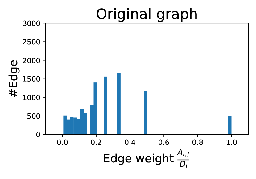
(a) Original edge weight of Cora.

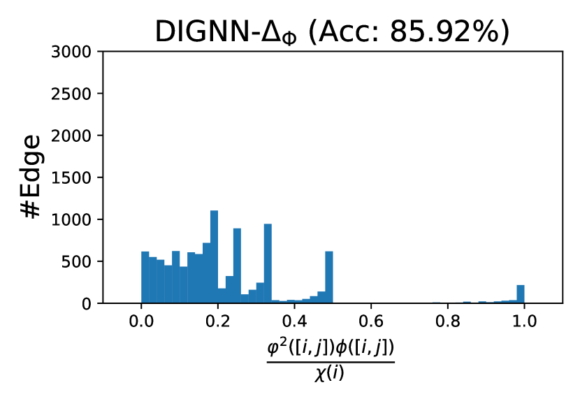
(b) Learned $\chi,\phi,\varphi$ for Cora.

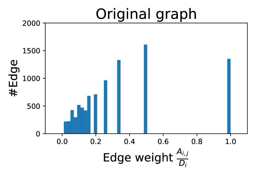
(c) Original edge weight of CiteSeer.

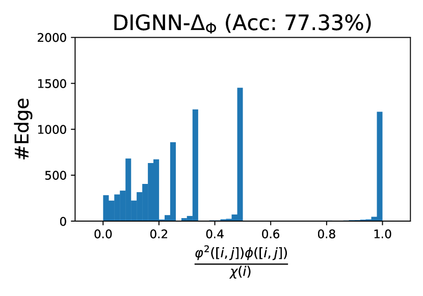
(d) Learned $\chi,\phi,\varphi$ for CiteSeer.

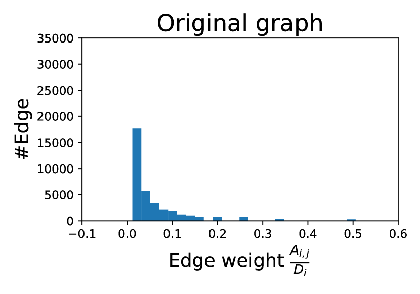
(e) Original edge weight of Chameleon.

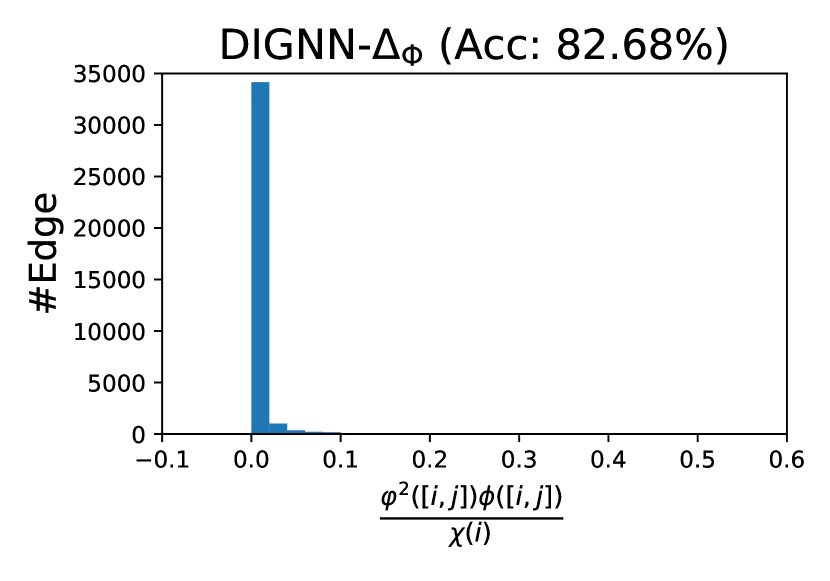
(f) Learned $\chi,\phi,\varphi$ for Chameleon.

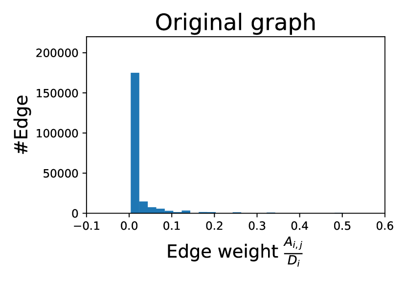
(g) Original edge weight of Squirrel.

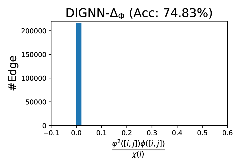
(h) Learned $\chi,\phi,\varphi$ for Squirrel.

Figure 4: Results for the learned graph metric.

F.3 Results for the learned positive real-valued functions

Here, we compare the values induced by the learned positive real-valued functions and the values induced by the original edge weights for several heterophilic and homophilic benchmark datasets. We present the distributions of the values of $\frac{\varphi^{2}([i,j])\phi([i,j])}{\chi(i)}$ of DIGNN-$\Delta_{\Phi}$ over all edges and the distribution of original edge weights in Figure 4.

We observe from Figures 4(a), 4(b), 4(c) and 4(d) that the distributions of the values of $\frac{\varphi^{2}([i,j])\phi([i,j])}{\chi(i)}$ on homophilic benchmark datasets, i.e., Cora and CiteSeer, are similar to the distributions of original normalized edge weights, which indicates that aggregating and transforming node features over the original graph topology is highly beneficial for label prediction. It explains why our models and explicit GNN baselines archive similar performance on these homophilic benchmark datasets.

Contradict to the results of Figures 4(e), 4(f), 4(g) and 4(h) on homophilic graphs, the results on heterophilic graphs, i.e., Chameleon and Squirrel, show that the distributions of the values of $\frac{\varphi^{2}([i,j])\phi([i,j])}{\chi(i)}$ are substantially different from the distributions of the original edge weights. We observe that the values learned by DIGNN-$\Delta_{\Phi}$ are mostly close to zero for most edges, indicating that the propagation weights of DIGNN-$\Delta_{\Phi}$ are generally very small. It illustrates that the local neighborhood information in Chameleon and Squirrel is not as helpful for label prediction as it is in Cora and CiteSeer. Consequently, propagating and transforming node features over the original graph topology may hinder the performance of GNNs on these heterophilic datasets.

Appendix G Computational Complexity and Running Time of DIGNNs

G.1 Computational complexity of the implicit graph diffusion layer in DIGNN-$\Delta_{\Phi}$

Given a graph ${\mathcal{G}}=({\mathcal{V}},{\mathcal{E}},{\mathbf{A}})$ with $n$ vertices and $m$ edges (suppose that $m>n$), node embeddings $\widetilde{{\mathbf{X}}}=(\widetilde{{\mathbf{x}}}_{1},\dots,\widetilde{{\mathbf{x}}}_{n})^{\top}\in\mathbb{R}^{n\times d}$. Let parameters $\Theta_{\chi}\in\mathbb{R}^{h\times d},\Theta_{\phi}\in\mathbb{R}^{h\times h},\Theta_{\varphi}\in\mathbb{R}^{h\times d}$ and the positive real-valued functions $\chi,\phi,\varphi$ are defined as Eq. 12, 13 and 14 respectively, i.e., $\forall i\in{\mathcal{V}}$ and $\forall[i,j]\in{\mathcal{E}}$,

$$\chi(i)={} {D}_{i}\tanh(\|\Theta_{\chi}\widetilde{{\mathbf{x}}}_{i}\|),$$

$$\phi([i,j])={} \tanh(|(\Theta_{\phi}\Theta_{\chi}\widetilde{{\mathbf{x}}}_{i})^{\top}(\Theta_{\phi}\Theta_{\chi}\widetilde{{\mathbf{x}}}_{j})|),$$

$$\varphi([i,j])={} \sqrt{{A}_{i,j}\tanh((\|\Theta_{\varphi}(\widetilde{{\mathbf{x}}}_{i}-\widetilde{{\mathbf{x}}}_{j})\|+\epsilon)^{-1})},$$

Note that by Eq. 6:

$$(\Delta_{\Phi}f)(i)=\frac{1}{\chi(i)}\sum_{j=1}^{n}\varphi([i,j])^{2}\phi([i,j])\left(f(i)-f(j)\right).$$

for ${\mathbf{Z}}^{(t)}=({\mathbf{z}}_{1}^{(t)},\dots,{\mathbf{z}}_{n}^{(t)}),t=0,1,\dots,T$, we obtain

$$\left(\Delta_{\Phi}{\mathbf{Z}}^{(t)}\right)_{i,:}=\frac{1}{\chi(i)}\sum_{j=1}^{n}\varphi([i,j])^{2}\phi([i,j])\left({\mathbf{z}}_{i}^{(t)}-{\mathbf{z}}_{j}^{(t)}\right).$$

Consider the iteration equation Eq. 19 with $\Delta\equiv\Delta_{\Phi}$ that is used to solve the implicit GNN layer of DIGNN-$\Delta_{\Phi}$, i.e.,

$${\mathbf{Z}}^{(t+1)}=\widetilde{{\mathbf{X}}}-\frac{1}{\mu}\Delta_{\Phi}{\mathbf{Z}}^{(t)},\text{ with }{\mathbf{Z}}^{(0)}=\mathbf{0},t=0,1,\dots,T,$$

we break down its computational complexity analysis as follows:

• Computing $\chi(i)$: This involves a matrix-vector multiplication $\Theta_{\chi}\widetilde{{\mathbf{x}}}_{i}$ with complexity $O(hd)$, followed by a norm ($O(h)$) and an application of $\tanh$ ($O(h)$). The total complexity for computing $\chi(i)$ is $O(hd+h)=O(hd)$.

• Computing $\phi([i,j])$: This requires a matrix-vector multiplication $\Theta_{\phi}\Theta_{\chi}\widetilde{{\mathbf{x}}}_{i}$ with complexity $O(h^{2}+hd)$. Similarly for $\Theta_{\phi}\Theta_{\chi}\widetilde{{\mathbf{x}}}_{i}$ we we need $O(h^{2}+hd)$ and $(\Theta_{\phi}\Theta_{\chi}\widetilde{{\mathbf{x}}}_{i})^{\top}(\Theta_{\phi}\Theta_{\chi}\widetilde{{\mathbf{x}}}_{j})$ is $O(2(h^{2}+hd)+h^{2})=O(h^{2}+hd)$. The absolute value and $\tanh$ are $O(1)$ operations. The total complexity for computing $\phi([i,j])$ is $O(h^{2}+hd)$.

• Computing $\varphi([i,j])$: Similar to $\phi([i,j])$, but involves vector subtraction $O(d)$, a matrix-vector multiplication $\Theta_{\varphi}(\widetilde{{\mathbf{x}}}_{i}-\widetilde{{\mathbf{x}}}_{j})$ with complexity $O(hd)$, and a norm plus element-wise operations. Thus, the complexity is $O(hd)$.

• Computing $\Delta_{\Phi}{\mathbf{Z}}^{(t)}$: The dominant term comes from computing $\phi([i,j])$ for all $m$ edges, leading to $O(m(h^{2}+hd))$.

• Updating ${\mathbf{Z}}^{(t+1)}$: The update equation involves subtracting a matrix from another $O(n\times d)$ and scaling by $1/\mu$ with $O(n\times d)$, which is negligible compared to the complexity of computing $\Delta_{\Phi}{\mathbf{Z}}^{(t)}$.

Therefore, the total computational complexity per iteration is $O(m(h^{2}+hd))$. Since this update is repeated for $T$ iterations, the overall computational complexity of Eq. 19 is $O(Tm(h^{2}+hd))$.

G.2 Running time of DIGNNs

Table 8 reports the averaged running time of DIGNN-$\Delta^{\text{(rw)}}$ and DIGNN-$\Delta_{\Phi}$ on several benchmark datasets. Our experiments are conducted on a server equipped with a GeForce RTX 2080 Ti and 12GB of GPU memory.

Table 8: Running of DIGNNs on node classification datasets. Averaged running time per epoch (ms) / averaged total running time (s).

Method	Chameleon	Squirrel	Cora	CiteSeer	PubMed
DIGNN-$\Delta^{\text{(rw)}}$	22.38ms / 32.78s	60.58ms / 104.25s	22.02ms / 30.35s	23.79ms / 36.08s	34.82ms / 51.21s
DIGNN-$\Delta_{\Phi}$	38.89ms / 67.74s	133.46ms / 249.48s	28.92ms / 46.38s	30.95ms / 40.62s	71.11ms / 123.61s

References

- Atwood and Towsley, (2016) Atwood, J. and Towsley, D. (2016). Diffusion-convolutional neural networks. In Advances in Neural Information Processing Systems 29: Annual Conference on Neural Information Processing Systems 2016, December 5-10, 2016, Barcelona, Spain, pages 1993–2001.
- Bai et al., (2019) Bai, S., Kolter, J. Z., and Koltun, V. (2019). Deep equilibrium models. In Advances in Neural Information Processing Systems 32: Annual Conference on Neural Information Processing Systems 2019, NeurIPS 2019, December 8-14, 2019, Vancouver, BC, Canada, pages 688–699.
- Baker et al., (2023) Baker, J., Wang, Q., Hauck, C. D., and Wang, B. (2023). Implicit graph neural networks: A monotone operator viewpoint. In Krause, A., Brunskill, E., Cho, K., Engelhardt, B., Sabato, S., and Scarlett, J., editors, International Conference on Machine Learning, ICML 2023, 23-29 July 2023, Honolulu, Hawaii, USA, volume 202 of Proceedings of Machine Learning Research, pages 1521–1548. PMLR.
- Baranwal et al., (2021) Baranwal, A., Fountoulakis, K., and Jagannath, A. (2021). Graph convolution for semi-supervised classification: Improved linear separability and out-of-distribution generalization. In Proceedings of the 38th International Conference on Machine Learning, ICML 2021, 18-24 July 2021, Virtual Event, volume 139 of Proceedings of Machine Learning Research, pages 684–693. PMLR.
- Belkin et al., (2004) Belkin, M., Matveeva, I., and Niyogi, P. (2004). Regularization and semi-supervised learning on large graphs. In The 17th Annual Conference on Learning Theory, COLT 2004, Banff, Canada, July 1-4, 2004, volume 3120, pages 624–638.
- Belkin et al., (2006) Belkin, M., Niyogi, P., and Sindhwani, V. (2006). Manifold regularization: A geometric framework for learning from labeled and unlabeled examples. Journal of Machine Learning Research, 7:2399–2434.
- Bodnar et al., (2022) Bodnar, C., Giovanni, F. D., Chamberlain, B. P., Liò, P., and Bronstein, M. M. (2022). Neural sheaf diffusion: A topological perspective on heterophily and oversmoothing in gnns. CoRR, abs/2202.04579.
- (8) Chamberlain, B., Rowbottom, J., Eynard, D., Giovanni, F. D., Dong, X., and Bronstein, M. M. (2021a). Beltrami flow and neural diffusion on graphs. In Advances in Neural Information Processing Systems 34: Annual Conference on Neural Information Processing Systems 2021, NeurIPS 2021, December 6-14, 2021, pages 1594–1609.
- (9) Chamberlain, B., Rowbottom, J., Gorinova, M. I., Bronstein, M. M., Webb, S., and Rossi, E. (2021b). GRAND: graph neural diffusion. In Proceedings of the 38th International Conference on Machine Learning, ICML 2021, 18-24 July 2021, volume 139 of Proceedings of Machine Learning Research, pages 1407–1418. PMLR.
- Chen et al., (2020) Chen, M., Wei, Z., Huang, Z., Ding, B., and Li, Y. (2020). Simple and deep graph convolutional networks. In Proceedings of the 37th International Conference on Machine Learning, ICML 2020, 13-18 July 2020, Virtual Event, volume 119 of Proceedings of Machine Learning Research, pages 1725–1735. PMLR.
- Chen et al., (2022) Chen, Q., Wang, Y., Wang, Y., Yang, J., and Lin, Z. (2022). Optimization-induced graph implicit nonlinear diffusion. In International Conference on Machine Learning, ICML 2022, 17-23 July 2022, Baltimore, Maryland, USA, volume 162 of Proceedings of Machine Learning Research, pages 3648–3661. PMLR.
- Chen et al., (2018) Chen, T. Q., Rubanova, Y., Bettencourt, J., and Duvenaud, D. (2018). Neural ordinary differential equations. In Advances in Neural Information Processing Systems 31: Annual Conference on Neural Information Processing Systems 2018, NeurIPS 2018, December 3-8, 2018, Montréal, Canada, pages 6572–6583.
- Chien et al., (2021) Chien, E., Peng, J., Li, P., and Milenkovic, O. (2021). Adaptive universal generalized pagerank graph neural network. In 9th International Conference on Learning Representations, ICLR 2021, Virtual Event, Austria, May 3-7, 2021. OpenReview.net.
- Chung, (1997) Chung, F. R. (1997). Spectral graph theory, volume 92. American Mathematical Society.
- Cong et al., (2021) Cong, W., Ramezani, M., and Mahdavi, M. (2021). On provable benefits of depth in training graph convolutional networks. In Advances in Neural Information Processing Systems 34: Annual Conference on Neural Information Processing Systems 2021, NeurIPS 2021, December 6-14, 2021, virtual, pages 9936–9949.
- Defferrard et al., (2016) Defferrard, M., Bresson, X., and Vandergheynst, P. (2016). Convolutional neural networks on graphs with fast localized spectral filtering. In Advances in Neural Information Processing Systems 29, NIPS 2016, December 5-10, 2016, Barcelona, Spain, pages 3837–3845.
- Du et al., (2019) Du, S. S., Hou, K., Salakhutdinov, R., Póczos, B., Wang, R., and Xu, K. (2019). Graph neural tangent kernel: Fusing graph neural networks with graph kernels. In Advances in Neural Information Processing Systems 32: Annual Conference on Neural Information Processing Systems 2019, NeurIPS 2019, December 8-14, 2019, Vancouver, BC, Canada, pages 5724–5734.
- El-Yaniv and Pechyony, (2009) El-Yaniv, R. and Pechyony, D. (2009). Transductive rademacher complexity and its applications. Journal of Artificial Intelligence Research, 35:193–234.
- Eliasof et al., (2021) Eliasof, M., Haber, E., and Treister, E. (2021). PDE-GCN: novel architectures for graph neural networks motivated by partial differential equations. In Advances in Neural Information Processing Systems 34: Annual Conference on Neural Information Processing Systems 2021, NeurIPS 2021, December 6-14, 2021, virtual, pages 3836–3849.
- Esser et al., (2021) Esser, P. M., Vankadara, L. C., and Ghoshdastidar, D. (2021). Learning theory can (sometimes) explain generalisation in graph neural networks. In Advances in Neural Information Processing Systems 34: Annual Conference on Neural Information Processing Systems 2021, NeurIPS 2021, December 6-14, 2021, virtual, pages 27043–27056.
- Fey and Lenssen, (2019) Fey, M. and Lenssen, J. E. (2019). Fast graph representation learning with pytorch geometric. CoRR, abs/1903.02428.
- Fu et al., (2022) Fu, G., Zhao, P., and Bian, Y. (2022). p-laplacian based graph neural networks. In International Conference on Machine Learning, ICML 2022, 17-23 July 2022, Baltimore, Maryland, USA, volume 162 of Proceedings of Machine Learning Research, pages 6878–6917. PMLR.
- Gallicchio and Micheli, (2020) Gallicchio, C. and Micheli, A. (2020). Fast and deep graph neural networks. In The Thirty-Fourth AAAI Conference on Artificial Intelligence, AAAI 2020, The Thirty-Second Innovative Applications of Artificial Intelligence Conference, IAAI 2020, The Tenth AAAI Symposium on Educational Advances in Artificial Intelligence, EAAI 2020, New York, NY, USA, February 7-12, 2020, pages 3898–3905. AAAI Press.
- Garg et al., (2020) Garg, V. K., Jegelka, S., and Jaakkola, T. S. (2020). Generalization and representational limits of graph neural networks. In Proceedings of the 37th International Conference on Machine Learning, ICML 2020, 13-18 July 2020, Virtual Event, volume 119 of Proceedings of Machine Learning Research, pages 3419–3430. PMLR.
- Ghaoui et al., (2019) Ghaoui, L. E., Gu, F., Travacca, B., and Askari, A. (2019). Implicit deep learning. CoRR, abs/1908.06315.
- Gilmer et al., (2017) Gilmer, J., Schoenholz, S. S., Riley, P. F., Vinyals, O., and Dahl, G. E. (2017). Neural message passing for quantum chemistry. In Proceedings of the 34th International Conference on Machine Learning, ICML 2017, Sydney, NSW, Australia, 6-11 August 2017, volume 70 of Proceedings of Machine Learning Research, pages 1263–1272. PMLR.
- Giovanni et al., (2022) Giovanni, F. D., Rowbottom, J., Chamberlain, B. P., Markovich, T., and Bronstein, M. M. (2022). Graph neural networks as gradient flows. CoRR, abs/2206.10991.
- Gu et al., (2020) Gu, F., Chang, H., Zhu, W., Sojoudi, S., and Ghaoui, L. E. (2020). Implicit graph neural networks. In Advances in Neural Information Processing Systems 33: Annual Conference on Neural Information Processing Systems 2020, NeurIPS 2020, December 6-12, 2020, virtual.
- Hamilton et al., (2017) Hamilton, W. L., Ying, Z., and Leskovec, J. (2017). Inductive representation learning on large graphs. In Advances in Neural Information Processing Systems 30: Annual Conference on Neural Information Processing Systems 2017, December 4-9, 2017, Long Beach, CA, USA, pages 1024–1034.
- Hein et al., (2007) Hein, M., Audibert, J., and von Luxburg, U. (2007). Graph laplacians and their convergence on random neighborhood graphs. Journal of Machine Learning Research, 8:1325–1368.
- Ju et al., (2023) Ju, H., Li, D., Sharma, A., and Zhang, H. R. (2023). Generalization in graph neural networks: Improved pac-bayesian bounds on graph diffusion. In International Conference on Artificial Intelligence and Statistics, 25-27 April 2023, Palau de Congressos, Valencia, Spain, volume 206 of Proceedings of Machine Learning Research, pages 6314–6341. PMLR.
- Keriven, (2022) Keriven, N. (2022). Not too little, not too much: a theoretical analysis of graph (over)smoothing. In NeurIPS.
- Kidger, (2022) Kidger, P. (2022). On neural differential equations. CoRR, abs/2202.02435.
- Kipf and Welling, (2017) Kipf, T. N. and Welling, M. (2017). Semi-supervised classification with graph convolutional networks. In 5th International Conference on Learning Representations, ICLR 2017, Toulon, France, April 24-26, 2017, Conference Track Proceedings. OpenReview.net.
- (35) Klicpera, J., Bojchevski, A., and Günnemann, S. (2019a). Predict then propagate: Graph neural networks meet personalized pagerank. In 7th International Conference on Learning Representations, ICLR 2019, New Orleans, LA, USA, May 6-9, 2019. OpenReview.net.
- (36) Klicpera, J., Weißenberger, S., and Günnemann, S. (2019b). Diffusion improves graph learning. In Advances in Neural Information Processing Systems 32: Annual Conference on Neural Information Processing Systems 2019, NeurIPS 2019, December 8-14, 2019, Vancouver, BC, Canada, pages 13333–13345.
- Krantz and Parks, (2002) Krantz, S. G. and Parks, H. R. (2002). The implicit function theorem: history, theory, and applications. Springer Science & Business Media.
- Ledoux and Talagrand, (1991) Ledoux, M. and Talagrand, M. (1991). Probability in Banach Spaces: isoperimetry and processes, volume 23. Springer Science & Business Media.
- Li et al., (2022) Li, H., Wang, M., Liu, S., Chen, P., and Xiong, J. (2022). Generalization guarantee of training graph convolutional networks with graph topology sampling. In International Conference on Machine Learning, ICML 2022, 17-23 July 2022, Baltimore, Maryland, USA, volume 162 of Proceedings of Machine Learning Research, pages 13014–13051. PMLR.
- Li et al., (2018) Li, Q., Han, Z., and Wu, X. (2018). Deeper insights into graph convolutional networks for semi-supervised learning. In Thirty-Second AAAI Conference on Artificial Intelligence, AAAI 2018, New Orleans, Louisiana, USA, February 2-7, 2018, pages 3538–3545.
- Liao et al., (2021) Liao, R., Urtasun, R., and Zemel, R. S. (2021). A pac-bayesian approach to generalization bounds for graph neural networks. In 9th International Conference on Learning Representations, ICLR 2021, Virtual Event, Austria, May 3-7, 2021. OpenReview.net.
- Liao et al., (2019) Liao, R., Zhao, Z., Urtasun, R., and Zemel, R. S. (2019). Lanczosnet: Multi-scale deep graph convolutional networks. In 7th International Conference on Learning Representations, ICLR 2019, New Orleans, LA, USA, May 6-9, 2019. OpenReview.net.
- Lim et al., (2021) Lim, D., Hohne, F., Li, X., Huang, S. L., Gupta, V., Bhalerao, O., and Lim, S. (2021). Large scale learning on non-homophilous graphs: New benchmarks and strong simple methods. In Advances in Neural Information Processing Systems 34: Annual Conference on Neural Information Processing Systems 2021, NeurIPS 2021, December 6-14, 2021, virtual, pages 20887–20902.
- Liu et al., (2022) Liu, J., Hooi, B., Kawaguchi, K., and Xiao, X. (2022). MGNNI: multiscale graph neural networks with implicit layers. In NeurIPS.
- Liu et al., (2021) Liu, J., Kawaguchi, K., Hooi, B., Wang, Y., and Xiao, X. (2021). EIGNN: efficient infinite-depth graph neural networks. In Advances in Neural Information Processing Systems 34: Annual Conference on Neural Information Processing Systems 2021, NeurIPS 2021, December 6-14, 2021, virtual, pages 18762–18773.
- Macedo and Oliveira, (2013) Macedo, H. D. and Oliveira, J. N. (2013). Typing linear algebra: A biproduct-oriented approach. Science of Computer Programming, 78(11):2160–2191.
- Maskey et al., (2022) Maskey, S., Levie, R., Lee, Y., and Kutyniok, G. (2022). Generalization analysis of message passing neural networks on large random graphs. In Advances in Neural Information Processing Systems 35: Annual Conference on Neural Information Processing Systems 2022, NeurIPS 2022, New Orleans, LA, USA, November 28 - December 9, 2022.
- Meyn and Tweedie, (2012) Meyn, S. P. and Tweedie, R. L. (2012). Markov chains and stochastic stability. Springer Science & Business Media.
- Mohri et al., (2018) Mohri, M., Rostamizadeh, A., and Talwalkar, A. (2018). Foundations of machine learning. MIT press.
- Morris et al., (2020) Morris, C., Kriege, N. M., Bause, F., Kersting, K., Mutzel, P., and Neumann, M. (2020). Tudataset: A collection of benchmark datasets for learning with graphs. arXiv preprint arXiv:2007.08663.
- Nadler et al., (2009) Nadler, B., Srebro, N., and Zhou, X. (2009). Semi-supervised learning with the graph Laplacian: The limit of infinite unlabelled data. Advances in Neural Information Processing Systems, NIPS 2009, 22:1330–1338.
- Niyogi, (2013) Niyogi, P. (2013). Manifold regularization and semi-supervised learning: some theoretical analyses. Journal of Machine Learning Research, 14(1):1229–1250.
- (53) Oono, K. and Suzuki, T. (2020a). Graph neural networks exponentially lose expressive power for node classification. In 8th International Conference on Learning Representations, ICLR 2020, Addis Ababa, Ethiopia, April 26-30, 2020. OpenReview.net.
- (54) Oono, K. and Suzuki, T. (2020b). Optimization and generalization analysis of transduction through gradient boosting and application to multi-scale graph neural networks. In Advances in Neural Information Processing Systems 33: Annual Conference on Neural Information Processing Systems 2020, NeurIPS 2020, December 6-12, 2020, virtual.
- Park et al., (2022) Park, J., Choo, J., and Park, J. (2022). Convergent graph solvers. In The Tenth International Conference on Learning Representations, ICLR 2022, Virtual Event, April 25-29, 2022. OpenReview.net.
- Paszke et al., (2017) Paszke, A., Gross, S., Chintala, S., Chanan, G., Yang, E., DeVito, Z., Lin, Z., Desmaison, A., Antiga, L., and Lerer, A. (2017). Automatic differentiation in pytorch.
- Pei et al., (2020) Pei, H., Wei, B., Chang, K. C., Lei, Y., and Yang, B. (2020). Geom-gcn: Geometric graph convolutional networks. In 8th International Conference on Learning Representations, ICLR 2020, Addis Ababa, Ethiopia, April 26-30, 2020. OpenReview.net.
- Rozemberczki et al., (2021) Rozemberczki, B., Allen, C., and Sarkar, R. (2021). Multi-scale attributed node embedding. Journal of Complex Networks, 9(2).
- Scarselli et al., (2009) Scarselli, F., Gori, M., Tsoi, A. C., Hagenbuchner, M., and Monfardini, G. (2009). The graph neural network model. IEEE Transactions on Neural Networks, 20(1):61–80.
- Scarselli et al., (2018) Scarselli, F., Tsoi, A. C., and Hagenbuchner, M. (2018). The vapnik-chervonenkis dimension of graph and recursive neural networks. Neural Networks, 108:248–259.
- Sen et al., (2008) Sen, P., Namata, G., Bilgic, M., Getoor, L., Gallagher, B., and Eliassi-Rad, T. (2008). Collective classification in network data. AI Magazine, 29(3):93–106.
- Shalev-Shwartz and Ben-David, (2014) Shalev-Shwartz, S. and Ben-David, S. (2014). Understanding machine learning: From theory to algorithms. Cambridge university press.
- Slepcev and Thorpe, (2017) Slepcev, D. and Thorpe, M. (2017). Analysis of $p$-laplacian regularization in semi-supervised learning. CoRR, abs/1707.06213.
- Smola and Kondor, (2003) Smola, A. J. and Kondor, R. (2003). Kernels and regularization on graphs. In Computational Learning Theory and Kernel Machines, 16th Annual Conference on Computational Learning Theory and 7th Kernel Workshop, COLT/Kernel 2003, Washington, DC, USA, August 24-27, 2003, Proceedings, volume 2777 of Lecture Notes in Computer Science, pages 144–158. Springer.
- Tang and Liu, (2023) Tang, H. and Liu, Y. (2023). Towards understanding generalization of graph neural networks. In Proceedings of the 40th International Conference on Machine Learning, volume 202 of Proceedings of Machine Learning Research, pages 33674–33719. PMLR.
- Thekumparampil et al., (2018) Thekumparampil, K. K., Wang, C., Oh, S., and Li, L. (2018). Attention-based graph neural network for semi-supervised learning. CoRR, abs/1803.03735.
- Thorpe et al., (2022) Thorpe, M., Nguyen, T. M., Xia, H., Strohmer, T., Bertozzi, A. L., Osher, S. J., and Wang, B. (2022). GRAND++: graph neural diffusion with A source term. In The Tenth International Conference on Learning Representations, ICLR 2022, Virtual Event, April 25-29, 2022. OpenReview.net.
- van Engelen and Hoos, (2020) van Engelen, J. E. and Hoos, H. H. (2020). A survey on semi-supervised learning. Machine Learning, 109(2):373–440.
- Velickovic et al., (2018) Velickovic, P., Cucurull, G., Casanova, A., Romero, A., Liò, P., and Bengio, Y. (2018). Graph attention networks. In 6th International Conference on Learning Representations, ICLR 2018, Vancouver, BC, Canada, April 30 - May 3, 2018, Conference Track Proceedings. OpenReview.net.
- Verma and Zhang, (2019) Verma, S. and Zhang, Z. (2019). Stability and generalization of graph convolutional neural networks. In Proceedings of the 25th ACM SIGKDD International Conference on Knowledge Discovery & Data Mining, KDD 2019, Anchorage, AK, USA, August 4-8, 2019, pages 1539–1548. ACM.
- Wang et al., (2021) Wang, Y., Wang, Y., Yang, J., and Lin, Z. (2021). Dissecting the diffusion process in linear graph convolutional networks. In Advances in Neural Information Processing Systems 34: Annual Conference on Neural Information Processing Systems 2021, NeurIPS 2021, December 6-14, 2021, virtual, pages 5758–5769.
- Weihs and Thorpe, (2023) Weihs, A. and Thorpe, M. (2023). Consistency of fractional graph-laplacian regularization in semi-supervised learning with finite labels. CoRR, abs/2303.07818.
- Wu et al., (2023) Wu, X., Chen, Z., Wang, W. W., and Jadbabaie, A. (2023). A non-asymptotic analysis of oversmoothing in graph neural networks. In The Eleventh International Conference on Learning Representations, ICLR 2023, Kigali, Rwanda, May 1-5, 2023. OpenReview.net.
- Xhonneux et al., (2020) Xhonneux, L. A. C., Qu, M., and Tang, J. (2020). Continuous graph neural networks. In Proceedings of the 37th International Conference on Machine Learning, ICML 2020, 13-18 July 2020, Virtual Event, volume 119 of Proceedings of Machine Learning Research, pages 10432–10441. PMLR.
- Xie et al., (2023) Xie, X., Wang, Q., Ling, Z., Li, X., Liu, G., and Lin, Z. (2023). Optimization induced equilibrium networks: An explicit optimization perspective for understanding equilibrium models. IEEE Transactions on Pattern Analysis and Machine Intelligence, 45(3):3604–3616.
- Xu et al., (2019) Xu, K., Hu, W., Leskovec, J., and Jegelka, S. (2019). How powerful are graph neural networks? In 7th International Conference on Learning Representations, ICLR 2019, New Orleans, LA, USA, May 6-9, 2019. OpenReview.net.
- Yanardag and Vishwanathan, (2015) Yanardag, P. and Vishwanathan, S. V. N. (2015). Deep graph kernels. In Proceedings of the 21th ACM SIGKDD International Conference on Knowledge Discovery and Data Mining, Sydney, NSW, Australia, August 10-13, 2015, pages 1365–1374. ACM.
- Yehudai et al., (2021) Yehudai, G., Fetaya, E., Meirom, E. A., Chechik, G., and Maron, H. (2021). From local structures to size generalization in graph neural networks. In Proceedings of the 38th International Conference on Machine Learning, ICML 2021, 18-24 July 2021, Virtual Event, volume 139 of Proceedings of Machine Learning Research, pages 11975–11986. PMLR.
- Zhang et al., (2018) Zhang, M., Cui, Z., Neumann, M., and Chen, Y. (2018). An end-to-end deep learning architecture for graph classification. In Proceedings of the Thirty-Second AAAI Conference on Artificial Intelligence, (AAAI-18), the 30th innovative Applications of Artificial Intelligence (IAAI-18), and the 8th AAAI Symposium on Educational Advances in Artificial Intelligence (EAAI-18), New Orleans, Louisiana, USA, February 2-7, 2018, pages 4438–4445. AAAI Press.
- Zhao and Akoglu, (2020) Zhao, L. and Akoglu, L. (2020). Pairnorm: Tackling oversmoothing in gnns. In 8th International Conference on Learning Representations, ICLR 2020, Addis Ababa, Ethiopia, April 26-30, 2020. OpenReview.net.
- Zhou et al., (2004) Zhou, D., Bousquet, O., Lal, T. N., Weston, J., and Schölkopf, B. (2004). Learning with local and global consistency. In Advances in Neural Information Processing Systems 16, NIPS 2004, December 8-13, 2004, Vancouver and Whistler, British Columbia, Canada], pages 321–328. MIT Press.
- Zhou and Schölkopf, (2005) Zhou, D. and Schölkopf, B. (2005). Regularization on discrete spaces. In The 27th DAGM Symposium, Vienna, Austria, August 31 - September 2, 2005, volume 3663, pages 361–368.
- Zhou et al., (2021) Zhou, K., Dong, Y., Wang, K., Lee, W. S., Hooi, B., Xu, H., and Feng, J. (2021). Understanding and resolving performance degradation in deep graph convolutional networks. In CIKM ’21: The 30th ACM International Conference on Information and Knowledge Management, Virtual Event, Queensland, Australia, November 1 - 5, 2021, pages 2728–2737. ACM.
- Zhou and Wang, (2021) Zhou, X. and Wang, H. (2021). The generalization error of graph convolutional networks may enlarge with more layers. Neurocomputing, 424:97–106.
- Zhu et al., (2020) Zhu, J., Yan, Y., Zhao, L., Heimann, M., Akoglu, L., and Koutra, D. (2020). Beyond homophily in graph neural networks: Current limitations and effective designs. In Advances in Neural Information Processing Systems 33: Annual Conference on Neural Information Processing Systems 2020, NeurIPS 2020, December 6-12, 2020, virtual.
- Zhu et al., (2003) Zhu, X., Ghahramani, Z., and Lafferty, J. D. (2003). Semi-supervised learning using gaussian fields and harmonic functions. In Machine Learning, Proceedings of the Twentieth International Conference, ICML 2003, August 21-24, 2003, Washington, DC, USA, pages 912–919. AAAI Press.
- Zhu, (2005) Zhu, X. J. (2005). Semi-supervised learning literature survey.
- Zitnik and Leskovec, (2017) Zitnik, M. and Leskovec, J. (2017). Predicting multicellular function through multi-layer tissue networks. Bioinformatics, 33(14):i190–i198.