The Galaxy Number Density Profile of Haloes

Abstract

More precise measurements of galaxy clustering will be provided by the next generation of galaxy surveys such as DESI, WALLABY and SKA. To utilize this information to improve our understanding of the Universe, we need to accurately model the distribution of galaxies in their host dark matter halos. In this work we present a new galaxy number density profile of haloes, which makes predictions for the positions of galaxies in the host halo, different to the widely adopted Navarro–Frenk–White (NFW) profile, since galaxies tend to be found more in the outskirts of halos (nearer the virial radius) than an NFW profile. The parameterised galaxy number density profile model of haloes is fit and tested using the Dark Sage semi-analytic model of galaxy formation. We find that our galaxy number density profile model of haloes can accurately reproduce the halo occupation distribution and galaxy two-point correlation function of the Dark Sage simulation. We also derive the analytic expressions for the circular velocity and gravitational potential energy for this profile model. We use the SDSS DR10 galaxy group catalogue to validate this galaxy number density profile model of haloes. Compared to the NFW profile, we find that our model more accurately predicts the positions of galaxies in their host halo and the galaxy two-point correlation function.

1 Introduction

Many galaxies tend to gather in groups/clusters of several members, and a group of galaxies will inhabit a dark matter halo, for which the dark matter dominates the mass of this system. In a group, the most massive or luminous galaxy is identified as the central galaxy, which typically resides in the center of the host halo gravitational potential (Yang et al., 2013; Wetzel et al., 2013; Li et al., 2014), while the rest of the galaxies are labelled ‘satellites’. Studying the galaxy–halo connection and density profile of halos enables us to understand the formation and evolution of galaxies and constrain cosmological models (White & Rees, 1978; Lacey & Cole, 1993; Cole et al., 2000; Bell et al., 2003; Fontanot et al., 2009).

There have been many different density profiles of halos developed to model the dark matter distribution in halos, and they are well reviewed by Keeton (2001) and Cooray & Sheth (2002). Among these models, the most commonly used model is the Navarro–Frenk–White (NFW) density profile (Navarro et al., 1996, 1997). There have been also some modified NFW profile models developed in past works, for example, the modified NFW profile in Maller & Bullock (2004) and the cuspy profile (Moore, 1994; Kravtsov et al., 1998; Moore et al., 1999). Some other well known dark matter density profiles of haloes are the Hernquist profile (Hernquist, 1990) and the singular isothermal sphere profile (Sheth et al., 2001). In addition to model the dark matter distribution, an exponential profile (Padmanabhan et al., 2017) has been used to model the distribution of neutral atomic hydrogen (H i) gas in a halo. Particularly, there have been also several works that have studied the dark matter halo shape of a single galaxy; for example, O’Brien et al. (2010) used the pseudo-isothermal sphere profile to model the dark matter halo of galaxy UGC 7321. However, in cosmology, we are only interested in the halo models that describe the distribution of galaxies in groups and clusters, which need not match that of the total dark matter.

In cosmological large-scale structure analysis, mock catalogues of real galaxy surveys are required to estimate the errors of inferred cosmological parameters and identify possible systematics in the data and analysis methods. Mock surveys are often constructed with a halo occupation distribution model (HOD). In an HOD, a galaxy number density profile of haloes must be used to assign positions and velocities to mock galaxies inside the halo. In a significant number of previous works, the galaxy number density profile of haloes has been assume to be the same as the dark matter density profile of haloes, or the radial distribution of galaxies in a halo has been assumed to follow the total dark matter, modelled by the NFW profile (e.g. Guo et al., 2014, 2015; Howlett et al., 2015, 2022; Qin et al., 2019, 2021; Alam et al., 2020; Avila et al., 2020; Paranjape et al., 2021).

However, other recent research indicates that galaxies tend to be found more in the outskirts of halos (nearer the virial radius) than an NFW profile, implying their distribution is not the same as the dark matter. For example, Avila et al. (2020) used the eBOSS survey to fit the HOD model, they found that to optimize the HOD models to reproduce the galaxy clustering, the NFW profile has to be modified. Using simulations, Orsi & Angulo (2018) find that the emission line galaxies tend to be found in the outskirts of halos. Other examples can be found in Guo et al. (2014); Chen et al. (2017); Kraljic et al. (2018); Qin et al. (2022). As a consequence, the measured galaxy two-point correlation function on small separation scales agrees poorly with the prediction from profile models of haloes developed in the past works, such as the NFW profile (Qin et al. 2022, hereafter Q22 ). Chen & Afshordi (2023) study the distribution of dark matte, rather than galaxies, in the outskirts of halos, based on the dark matter simulation DarkEmu (Nishimichi et al., 2019), and this simulation does not account for any galaxy formation processes.

In addition, the study of the ‘lensing-is-low’ problem indicates that HOD models optimized to reproduce the clustering of galaxies over-predict their galaxy-galaxy lensing (Leauthaud et al., 2017). Using the IllustrisTNG (Pillepich et al., 2018) simulation, Chaves-Montero et al. (2023) find that the origin of the lensing-is-low problem may due to the fact that the galaxies are less concentrated than the prediction of NFW profile.

There has also been recent interest in the odd-multipole galaxy correlation function and power spectra (McDonald, 2009; Bonvin, 2014; Gaztanaga et al., 2017; Di Dio & Seljak, 2019; Beutler et al., 2019), such as the dipole and octopole of the correlation function/power spectrum. The higher multipole ($\ell>0$) statistics are generated by redshift-space distortion (RSD) effects, but the odd-multipoles are normally set to zero, assuming that RSD comes from only the quadratic Kaiser term. Non-zero odd-multipoles are generated by unequal gravitational potentials of different galaxies in the host halos, have been introduced as a method to constrain cosmological models. An incorrect galaxy number density profile of haloes will result in incorrect predictions of correlation function odd-multipole, and this will further bias the measurements of the cosmological parameters. Therefore, it is necessary to accurately model the galaxy number density profile of haloes.

In this paper, we use a simulated galaxy catalogue built with the Dark Sage semi-analytic model of galaxy formation (Stevens et al., 2018) to explore the functional form of the galaxy number density profile of haloes. This simulation doesn’t populate the halos with galaxies just using a particular density profile of haloes, but rather the distribution is a prediction as a result of numerous coupled galaxy evolution processes. We compare and validate this galaxy number density profile model of haloes against measurements from the group catalogue of Sloan Digital Sky Survey Data Release 10 (York et al., 2000; Ahn et al., 2014). Our galaxy number density profile of haloes will be used to generate mocks for the coming galaxy surveys, for example the Widefield ASKAP L-band Legacy All-sky Blind surveY (or WALLABY, Koribalski et al. 2020), the Dark Energy Spectroscopic Instrument (DESI, DESI Collaboration et al. 2016) and the Square Kilometre Array (SKA, Square Kilometre Array Cosmology Science Working Group et al. 2020).

In the past, there are less research on galaxy number density profile of haloes. Budzynski et al. (2012) only measured the projected (surface) galaxy density profiles (Bartelmann, 1996) of halos (using SDSS DR7), they did not develop any analytic models for the density profile and they only use the clusters with Luminous Red Galaxies at their centers for their measurements.

Our paper is structured as follows. In Section 2, we introduce the Dark Sage simulation and the SDSS DR10 group catalogue. In Section 3, we explore the functional form of the galaxy number density profile of haloes using Dark Sage. In Section 4, we fit the galaxy two-point correlation function and constrain the HOD for Dark Sage galaxies to validate our galaxy number density profile of haloes. In Section 5, we validate our galaxy number density profile of haloes using the SDSS DR10 group catalogue. We conclude in Section 6.

Hereafter, the capital letter $M\equiv\log_{10}(m/m_{\odot})$ denotes the logarithmic mass per unit solar mass $m_{\odot}$.

2 Simulation and Data

2.1 The DARK SAGE simulation

In this work, we use the Dark Sage semi-analytic model of galaxy formation (Stevens et al., 2016, 2018) to explore the functional form of the galaxy number density profile of haloes. The simulated galaxy catalogue from Dark Sage used in this paper is the same as the simulation used in Q22 .

Dark Sage builds and evolves galaxies within halo merger trees constructed from an $N$-body simulation. The 2018 model used here was run on the widely used Millennium simulation (Springel et al., 2005). This simulation assumes the $\Lambda$ cold dark matter model ($\Lambda$CDM) with cosmological parameters from the Wilkinson Microwave Anisotropy Probe (WMAP) First-Year results (Spergel et al., 2003), with matter density $\Omega_{\rm m}=0.25$, dark energy density $\Omega_{\Lambda}=0.75$, and Hubble parameter $h=0.73$ (where $H_{0}=100$ $h$ km s^-1 Mpc^-1). The comoving box size of the simulation is $500\,h^{-1}$ Mpc.

Dark Sage accounts for gas accretion and cooling, star formation, stellar feedback, gravitational disc instabilities, central black-hole growth, active galactic nuclei feedback, environmental stripping of gas, and galaxy mergers. Among other observational constraints, Dark Sage was calibrated to reproduce the H i-to-stellar mass ratio (Brown et al., 2015) and H i mass function (Zwaan et al., 2005; Martin et al., 2010) with its eight free parameters (Stevens et al., 2018). In Dark Sage, all halos originally start with a galaxy at the centre, but the complicated merger history between halos of different masses as well as the secular and co-evolution of galaxies leads to some of those galaxies becoming satellites in larger halos with a radial dependence that is not easy to predict from first principles. In this paper, we apply a halo mass cut $M=11.7$ to the Dark Sage catalogue to remove the halos that are below the simulation resolution. The halo mass range of Dark Sage  can cover the halo mass range of DESI $M\in[12,14.5]$ (Wang et al., 2022; Yuan et al., 2023; Rocher et al., 2023). In addition, as discussed in Section 2 of Q22 , the halo mass range of Dark Sage  can also cover WALLABY.

2.2 The galaxy group catalogue from SDSS DR10

To measure the radial distribution of satellite galaxies in halos from real data for validation and comparison purposes, we use the galaxy group/cluster catalogue of Tempel et al. (2014a). The group catalogue (Tempel et al., 2014b) is mainly based on the Sloan Digital Sky Survey (SDSS) Data Release 10 (DR10, York et al. 2000; Ahn et al. 2014).

The primary sample for the group catalogue was taken from the SpecObj, bestobjid and fluxobjid tables, which can be downloaded from the Catalogue Archive Server of the SDSS (Tempel et al., 2014a). Due to fiber collisions of the instrument, the SDSS galaxy sample is not complete (Tempel et al., 2014a). Therefore, there are 1119 galaxies from the Two Micron All Sky Survey (2MASS, Jarrett et al. 2003) Redshift Survey (2MRS Huchra et al. 2012), 3494 galaxies from the Two-degree Field Galaxy Redshift Survey (2dFGRS, Colless et al. 2001, 2003) as well as 280 galaxies from the Third Reference Catalogue of Bright Galaxies (RC3, Corwin et al. 1994) that have been added to complement the SDSS sample. The final sample totals 588 193 galaxies, upon which the group catalogue was constructed.

A friends-of-friends (FoF) algorithm was implemented by Tempel et al. (2014a) to identify the galaxy groups. In this paper, we use a volume-limited catalogue of Tempel et al. (2014a). As mentioned in Tempel et al. (2014a), since in the volume-limited catalogue, the number density of galaxies is a constant by definition, therefore should be used to make comparison with simulations.

In the volume-limited catalogues, the absolute magnitude of galaxies was transformed from their apparent magnitude using the group mean redshift (Tempel et al., 2014a). A $k$-correction and evolution-correction have also been applied to the data. To suppress the redshift-space distortion (RSD, or the Finger-of-God effect, Kaiser 1987), the group mean distances were assigned to their member galaxies. The 3D Cartesian comoving positions of the galaxies have been accordingly calculated (Tempel et al., 2014a). These positions will be used to measure the halo density profile for galaxies in our paper. The line-of-sight peculiar velocities of galaxies were determined from the group mean distances and the observed redshift of the galaxies (Tempel et al., 2014a).

Assuming that galaxy groups inhabit common dark matter halos, the total mass of a group (or halo) is calculated using

$$m=2.325\times 10^{12}\frac{R_{g}}{\rm Mpc}\left(\frac{\sigma_{v}}{\rm 100~{}km~{}s^{-1}}\right)^{2}m_{\sun}\,,$$ (1)

which is derived from the virial theorem (Tempel et al., 2014a). In the above equation, $\sigma_{v}$ is the velocity dispersion (reflecting the average kinetic energy of the group members) which was estimated using the line-of-sight peculiar velocities of galaxies and the mean group velocity as well as the mean group redshift (Tempel et al., 2014a). $R_{g}$ is the gravitational radius (reflecting the average potential energy of the group members), which was calculated by assuming the total matter (rather than galaxies) in a halo is modelled by the NFW profile (Bartelmann, 1996; Łokas & Mamon, 2001; Tempel et al., 2014a). In the catalogue, group masses range from $10^{9}\,m_{\sun}$ to $10^{15}\,m_{\sun}$. We plot the halo mass function of SDSS data in Fig.1, as shown by the yellow dots, the halo mass function of SDSS drops down for $M<=13.5$ since the catalogue is not complete due to the fibre collision effects and luminosity limits in the observation. Therefore, in this paper, we only use the halos with $m>10^{13.5}\,m_{\sun}$ to measure the galaxy number density profile of haloes.

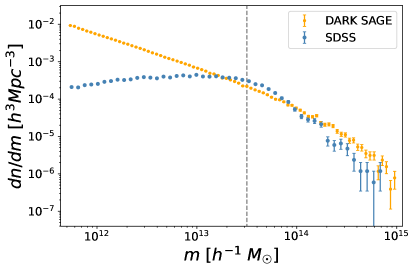
Figure 1: The halo mass function of SDSS (blue dots) and Dark Sage (yellow dots). Here we only intend to show the turning point of the halo mass function of SDSS.

Tempel et al. (2014a) created seven volume-limited catalogues with different absolute ($r$-band) magnitude cuts. In this paper, we use the catalogue with magnitude cut $-20.0$ since the redshift cut of this catalogue is 0.11, which is comparable to the redshift limit of WALLABY. There are 163 094 galaxies and 24 258 groups in the catalogue. The LL of the FoF algorithm was set to be 0.515 $h^{-1}$ Mpc (Tempel et al., 2014a).

The smallest groups in our data sample of choice contain only two galaxies. Around 52.1% of the galaxies are ‘isolated’ galaxies, meaning they are the sole occupant of their halo with no satellite galaxies. Since we want to measure the radial distribution of satellite galaxies in halos, the isolated galaxies are excluded in our research. In the catalogue, the galaxies with luminosity rank equal to one (the most luminous galaxies) are identified as the central galaxies (Tempel et al., 2014a).

3 The galaxy number density profile of haloes

3.1 The galaxy number density profile model of haloes

In the course of Q22 , we found that radial distribution of satellite galaxies within Dark Sage  was considerably wider than predicted by the NFW profile. As a result of that finding, assuming the halo is spherically symmetric, in this work we instead adopt the following function to model the satellite galaxy number density profile of haloes:

$$\rho_{g}(r)\propto r^{2}\exp\left[-\beta(cr)^{\alpha}\right]\,,$$ (2)

where $c\equiv R_{\mathrm{vir}}/R_{s}$ is the halo concentration. $R_{s}$ is the break radius between the outer and inner density profile of the halo. $R_{\rm vir}$ is the virial radius of a halo, it is computed from the halo virial mass $m$ using

$$R_{\mathrm{vir}}=\left(\frac{3m}{4\uppi\,\Delta\,\rho_{c}}\right)^{1/3}~{},$$ (3)

where $\Delta=200$ is the overdensity threshold of halo identification. $\rho_{c}=3H_{0}^{2}/(8\uppi G)$ is the critical density of the universe. $G$ is Newton’s gravitational constant. The parameters $\alpha$ and $\beta$ are functions of halo (virial) mass. Assuming the central galaxy sits at the center of potential of the halo, the radial distribution (probability density function) of satellite galaxies in a parent halo is then given by

$$f_{cs}(x)\propto\rho_{g}(r)\,r^{2}$$ (4)

(Zheng, 2004; Tinker et al., 2005; Zheng & Weinberg, 2007). $f_{cs}(x)$ should be normalized to 1 when integrating from $x=0$ to $x=1$, where $x\equiv r/(10R_{\rm vir})$. The number 10 is chosen to ensure the interval $[0,1]$ is large enough to cover the whole shape of the curves (see section 5.1 of Q22 for more discussion).

To explore the functional forms of $\alpha$ and $\beta$, we fit our model Eq. 2 to the measurements from Dark Sage  in 80 halo mass bins in the interval $M\in[11.7,15]$ (the mass bin width is around 0.04). We plot the measured $f_{cs}$ against $x$ in Fig. 2 for two example halo mass bins at each extreme of the range. The solid curves are the models fit to the measurements. All these $f_{cs}$ are normalized to integrate to one in the interval $x\in[0,1]$. The fit results of $\alpha$ and $\beta$ against the halo mass are shown in the blue dots of Fig. 3. We find a linear model fits the relation between $\alpha$ and halo mass $M$ very well;

$$\alpha=0.0778M-0.4419\,.$$ (5)

The fit result is shown in the yellow line in the top panel of Fig. 3. We use an exponential function to model the relation between $\beta$ and $M$, whose best fit is given by

$$\beta=3331.4392\exp\left[-0.5123M\right]\,,$$ (6)

This fit result is illustrated by the yellow curve in the bottom panel of Fig. 3. In all the above fitting procedures, we fit the measurements to the model curves (lines) by simply minimizing the least squares difference. The combination of Eq. 2, 5 and 6 comprise the density profile model we will adopt in this paper.

Figure 2: The probability density function (the radial distribution) of satellite galaxies $f_{cs}$ for two example halo mass bins. The pink and blue filled circles are the measurements from Dark Sage for halo mass bins centered on $M=11.73$, $14.86$ respectively. The solid curves are the models fit to the measurements. The dashed curves compare an NFW profile for these masses. All of them are normalized to integrate to one in the interval $x\in[0,1]$.

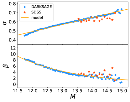
Figure 3: Top panel: blue dots show the $\alpha$ fitted by comparing the halo density profile model for galaxies Eq.2 to the measurements of Dark Sage in each halo mass bin. The yellow curve is the model Eq. 5 fit to the blue dots. Similarly, in the bottom panel, the blue dots show the fitted $\beta$ of the measurements of Dark Sage satellites in each halo mass bin, and the yellow curve is the Eq. 6 fit to the blue dots. In both cases, the red pentagrams are the results from SDSS data (see Section 5).

In Fig.2, the dashed curves depict the NFW profile for these masses assuming an one-to-one mass-concentration relation. The measured $f_{cs}$ of the galaxies from Dark Sage clearly does not agree with an NFW profile. Dark Sage  gives satellite galaxies that are found much closer to or beyond the Virial radius than would be predicted by the more centrally concentrated NFW profile.

As a more intuitive visual representation, we show in the left-hand panel of Fig. 4 gray dots that are randomly generated assuming our new galaxy number density profile model of haloes for $M=12$. The red curve illustrates the corresponding $f_{cs}$ of this halo mass. The light-blue circle indicates the position of the virial radius $R_{\rm vir}$ of the halo. Under our new model, satellite galaxies tend to be situated more in the outskirts of a halo. For comparison, the gray dots in the right-hand panel are generated assuming the NFW profile for the same halo mass (see Appendix A for relevant equations). Under the NFW profile, satellite galaxies are majorly concentrated within the virial radius and show no suppression at the halo center.

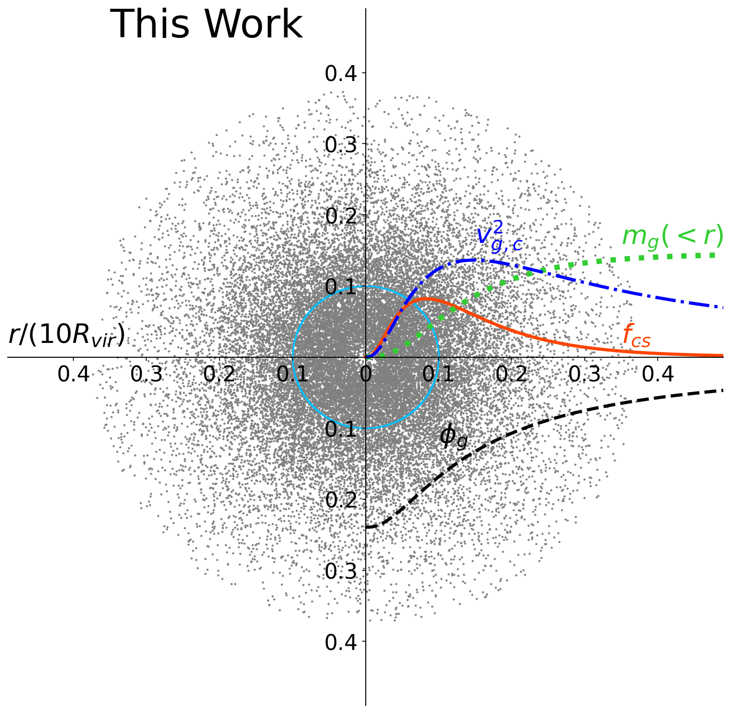
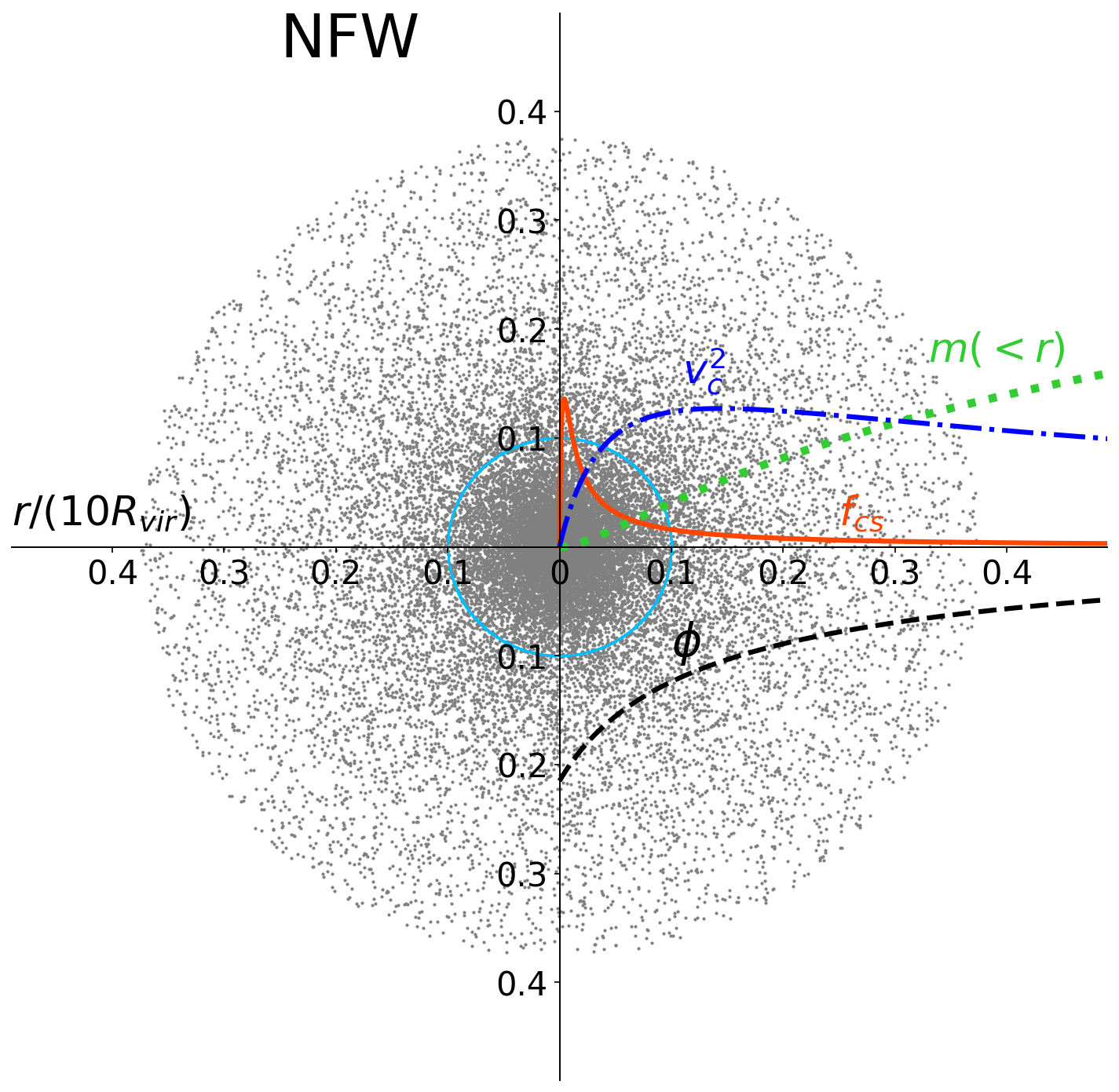
Figure 4: Comparing the profile model of Eq. 2 (left) to the NFW profile (right). The gray dots are random points generated based on these two density profile models for halo mass $M=12$. The light-blue circles indicate the virial radius of the halo mass $M=12$. The blue dashed-dotted curves illustrate the circular velocity $v^{2}_{c}$. The green dotted curves show the mass interior to $r$, i.e. $M(<r)$. The yellow dashed curves display the gravitational potential $\phi$. The red solid curves showcase the $f_{cs}$. The amplitudes of the curves are re-scaled in order to be visible in the same figure. The coordinates axis indicate the radial distances from the halo center, and are re-scaled to $r/(10R_{\rm vir})$.

There is also a physical motivation for a satellite PDF that peaks closer to $R_{\rm vir}$ than $R=0$. Galaxy orbits with a smaller radius relative to the centre of mass are not stable, as the galaxies are subject to a stronger tidal field and greater dynamical friction, meaning they will merge with the central galaxy and/or become stripped/disrupted over relatively short time-scales, and therefore cease to exist. However, though we can model these process using simulations, there are still challenges involved in identifying subhalos near halo centres in these simulations. The functional form we have selected in Eq. 2 is a phenomenological one based on Dark Sage, but we will later test/validate it against radial profiles of galaxy groups from SDSS data. For now, we have tested that this is not a specific feature of the Millennium simulation.

3.2 The convolution and Fourier transform for the galaxy number density profile of haloes

The probability density function (PDF) of satellite galaxy pairs in a parent halo is calculated from the convolution of a profile with another of exactly the same shape, given by (Sheth et al., 2001; Zheng & Weinberg, 2007)

$$f_{ss}(r)\,{\rm d}r\propto r^{2}\,{\rm d}r\int_{0}^{+\infty}\left[\tau_{1}^{2}\rho_{g}(\tau_{1})\int_{-1}^{1}\rho_{g}(\tau_{2})\,{\rm d}\mu\right]{\rm d}\tau_{1}\,,$$ (7)

where

$$\tau_{2}=\sqrt{\tau_{1}^{2}+r^{2}-2\tau_{1}\mu}$$ (8)

and ${\bf r}=\boldsymbol{\tau}_{2}-\boldsymbol{\tau}_{1}$ is the pair separation between position vectors $\boldsymbol{\tau}_{1}$ and $\boldsymbol{\tau}_{2}$. $\mu=-\cos\theta$, where $\theta$ is the angular between ${\bf r}$ and $\boldsymbol{\tau}_{1}$. $f_{ss}(x)$ should be normalized to 1 when integrating from $x=0$ to $x=1$.

Plugging Eq. 2 into Eq. 7, one can obtain

$$f_{ss}(r)\propto\frac{\beta^{-4r/\alpha}}{\alpha c^{4}}\int_{0}^{+\infty}\tau_{1}^{3}\exp[-\beta(c\tau_{1})^{\alpha}]~{}\times\\ \left[\Gamma\left(\frac{4}{a},~{}\beta c^{\alpha}|r-\tau_{1}|^{\alpha}\right)-\Gamma\left(\frac{4}{a},~{}\beta c^{\alpha}|r+\tau_{1}|^{\alpha}\right)\right]{\rm d}\tau_{1}\,,$$ (9)

where the regularized upper incomplete $\Gamma$ function is defined as:

$$\Gamma(A,x)\equiv\frac{1}{\Gamma(A)}\int_{x}^{+\infty}t^{A-1}\exp(-t)\,{\rm d}t$$ (10)

and where the complete $\Gamma$ function $\Gamma(A)\equiv\Gamma(A,0)$. Due to the $\Gamma$ functions inside the integral of Eq. 9, we can not solve the integration analytically. However, it can be solved using numerical methods easily; we first calculate a spline function for the term inside the integral, then calculate the integral numerically.

We plot the measured $f_{ss}$ (i.e. the PDF of satellite-satellite pairs measured in halo mass bins) against $x$ in Fig. 5, as shown in the circles for two example halo mass bins. The solid curves represent our new model. While the free parameters of our model were fitted to Dark Sage, the curves in Fig. 5 are not direct fits to the points in Fig. 5. This figure therefore validates the general applicability of our model with its fitted parameters. The dashed curves depict the NFW profile for these mass bins, which, again, clearly do not match the simulated data. All these $f_{ss}$ are normalized to integrate to one in the interval $x\in[0,1]$.

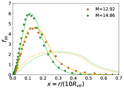
Figure 5: The probability density function (the radial distribution) of satellite galaxy pairs $f_{ss}$ for two example halo mass bins. The yellow and green filled circles are the measurements from Dark Sage for halo mass bins centered on $M=12.68$, $14.86$ respectively. The solid curves are the model calculated from Eq. 9, using the mass-dependent parameter values for $\alpha$ (Eq. 5) and $\beta$ (Eq. 6). The dashed curves showcase the NFW profile for these masses. All of them are normalized to integrate to one in the interval $x\in[0,1]$.

The Fourier transformation for the galaxy number density profile of haloes is defined as (Cooray & Sheth, 2002)

$$y_{g}(k)\equiv\int_{0}^{R_{\mathrm{vir}}}4\uppi R^{2}\frac{\sin(kR)}{kR}\frac{\rho_{g}(R)}{m}\,{\rm d}R\,.$$ (11)

Plugging Eq. 2 into the above, one can be calculate $y_{g}(k)$ numerically. We plot the measured $y_{g}$ in Fig. 6, as shown in the circles for two example halo mass bins. The solid curves compare the models directly calculated from Eqs 11, 2, 5 and 6. They agree with the measurements. This figure therefore validates the general applicability of our model with its fitted parameters. For reference, the dashed curves depict the NFW profile for these mass bins. All these $y_{g}$ are normalized to 1 at $k=0$.

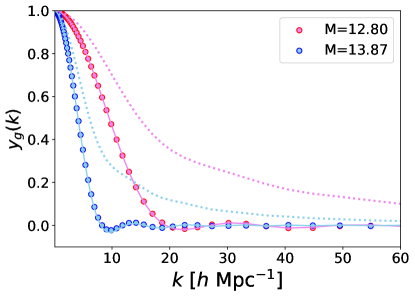
Figure 6: The Fourier transformation for the galaxy number density profile of haloes, in two example halo mass bins. The pink and blue filled circles are the measurements from Dark Sage for halo mass bins centered on $M=12.80$, $13.87$ respectively. The solid curves are the model calculated from Eqs 11 & 2, using the mass-dependent parameter values for $\alpha$ (Eq. 5) and $\beta$ (Eq. 6). The dashed curves showcase the NFW profile for these masses.

3.3 The dynamic properties

The galaxy number density profile of haloes of Eq. 2 is originally developed to model the distribution of galaxies. The dark matter in a halo is still assumed to be modeled by the NFW profile. The dynamic properties inferred from Eq. 2 can be treated as a perturbation term added upon the dynamic properties of the NFW profile. In this section, we will explore the dynamic properties corresponding to Eq. 2. For comparison, we also describe the dynamic properties of the NFW profile in Appendix A.

If $m_{g}$ denotes the mass of galaxies in a halo, we can normalize Eq. 2 to mass $m_{g}$ in the interval $r\in[0,~{}+\infty]$. The normalized galaxy number density profile of haloes is given by

$$\rho_{g}(r)=\frac{\alpha\beta^{\frac{5}{\alpha}}c^{5}m_{g}}{4\uppi\Gamma[\frac{5}{\alpha}]}r^{2}\exp\left[-\beta(cr)^{\alpha}\right]\,.$$ (12)

The circular velocity at a radial distance $r$ from the halo center is defined as (Sheth et al., 2001)

$$v^{2}_{c}\equiv\frac{Gm_{g}(<r)}{r}\,,$$ (13)

where the mass interior to $r$ is given by

$$m_{g}(<r)=4\uppi\int_{0}^{r}\tau^{2}\rho_{g}(\tau)d\tau\,.$$ (14)

Plugging Eq. 12 into the above equation yields

$$m_{g}(<r)=\frac{m_{g}}{\Gamma[\frac{5}{a}]}\left[\Gamma\left(\frac{5}{a}\right)-\Gamma\left(\frac{5}{a},~{}\beta c^{\alpha}r^{\alpha}\right)\right]\,.$$ (15)

Plugging the above into Eq. 13, one can obtain

$$v^{2}_{c,g}=\frac{Gm_{g}}{r\Gamma[\frac{5}{a}]}\left[\Gamma\left(\frac{5}{a}\right)-\Gamma\left(\frac{5}{a},~{}\beta c^{\alpha}r^{\alpha}\right)\right]\,,$$ (16)

which is the circular velocity for Eq. 12. In the left-hand panel of Fig. 4, the green-dotted curve displays the mass interior to $r$, the blue dash-dotted curve showcases the circular velocity. For comparison, the green-dotted curve in the right-hand panel shows the mass interior to $r$ for NFW profile. The blue dash-dotted curve showcases the circular velocity for NFW profile.

The gravitational potential energy at a radial distance $r$ from the halo center is given by (Sheth et al., 2001)

$$\phi_{g}(r)=\frac{-4\uppi G}{r}\int_{0}^{r}\tau^{2}\rho_{g}(\tau)d\tau-4\uppi G\int_{r}^{+\infty}\tau\rho_{g}(\tau)d\tau$$ (17)

Plugging Eq. 15 and Eq. 12 into the above equation, one can obtain

$$\begin{split}\phi_{g}(r)=&-\frac{Gm_{g}}{r\Gamma[\frac{5}{a}]}\bigg{[}\Gamma\left(\frac{5}{\alpha}\right)+\beta^{\frac{1}{\alpha}}cr\Gamma\left(\frac{4}{\alpha},~{}\beta c^{\alpha}r^{\alpha}\right)\\ &-\Gamma\left(\frac{5}{\alpha},~{}\beta c^{\alpha}r^{\alpha}\right)\bigg{]}\end{split}$$ (18)

which is the potential energy for Eq. 12. An example is illustrated by the black dashed curve of the left-hand-side panel of Fig. 4. For comparison, the black dashed curve in the right-hand-side panel shows the gravitational potential for NFW profile.

4 Validating the galaxy number density profile of haloes using the Dark Sage simulation

In this section we will explore whether or not our new galaxy number density profile model of haloes can correctly reproduce the galaxy two-point correlation function of Dark Sage galaxies.

4.1 The model of HOD and correlation function

In the HOD-based model, the galaxy two-point correlation function is computed as the combination of the ‘one-halo’ and ‘two-halo’ terms (Berlind & Weinberg, 2002; Yang et al., 2003; Zheng, 2004; Tinker et al., 2005; Guo et al., 2015; Zheng & Guo, 2016; Qin et al., 2022)

$$\xi_{gg}^{\rm mod}(r)=[1+\xi^{1h}_{gg}(r)]+\xi^{2h}_{gg}(r)~{},$$ (19)

where $r$ is the pair separation. The analytic expression of $\xi_{gg}^{\rm mod}$ in terms of an HOD model (or HOD parameters) and density profile model of haloes is fully presented in Section 4 of Q22 (or see Appendix B of Tinker et al. 2005). The expressions are lengthy, we therefore only briefly introduce them in the following texts rather than displaying the full expressions.

The ‘one-halo’ term $\xi^{1h}_{gg}$ is the contribution of intrahalo galaxy pairs, meaning it is sensitive to the halo density profile. The one-halo term is modeled as

$$\begin{split}1+\xi^{1h}_{gg}(r)=&\frac{1}{2\uppi\,r^{2}\,\bar{n}_{g}^{2}}\int_{0}^{\infty}\frac{1}{10R_{\mathrm{vir}}}\bigg{[}\left\langle N_{\mathrm{cen}}\,N_{\mathrm{sat}}\right\rangle\,f_{cs}(x)\\ +&\frac{\left\langle N_{\mathrm{sat}}(N_{\mathrm{sat}}-1)\right\rangle}{2}f_{ss}(x)\bigg{]}f_{h}(m)\,dm~{},\end{split}$$ (20)

where $\bar{n}_{g}$ is the average number density of galaxies, $f_{h}(m)$ is the model of the halo mass function.

The ‘two-halo’ term $\xi^{2h}_{gg}$ is the contribution of interhalo galaxy pairs and is therefore not sensitive to the halo density profile. The two-halo term is modeled as

$$\xi^{2h}_{gg}(r)=\left[1+\xi^{\prime}_{2h}(r)\right]\left(\frac{\bar{n}^{\prime}_{g}}{\bar{n}_{g}}\right)^{2}-1~{},$$ (21)

where

$$\xi^{\prime}_{2h}(r)=\frac{1}{2\uppi^{2}}\int_{0}^{\infty}b_{g}^{2}(k,r)\,P_{m}(k)\,k^{2}\,\frac{\sin(kr)}{kr}\,dk~{},$$ (22)

and where $\bar{n}^{\prime}_{g}$ is the average number density of galaxies that reside in halos with mass smaller than the so-called ‘halo exclusion’ limit. $b_{g}$ is galaxy biasing parameter. $P_{m}(k)$ is the nonlinear matter power spectrum.

The HOD of central galaxies of Dark Sage is given by $\langle N_{\mathrm{cen}}\rangle=1$ since Dark Sage requires that each parent halo hosts a central galaxy. We choose the following formula to model the HOD of satellite galaxies of Dark Sage (Zheng et al., 2007; Howlett et al., 2015; Guo et al., 2015; Zheng & Guo, 2016)

$$\langle N_{\mathrm{sat}}\rangle=\langle N_{\mathrm{cen}}\rangle\left(\frac{m-10^{M_{\mathrm{cut}}}}{10^{M_{1}}}\right)^{\beta}~{},$$ (23)

where the HOD parameters $M_{1}$, $\beta$ and $M_{\mathrm{cut}}$ will be fit by comparing the model correlation function $\xi_{gg}^{\rm mod}$ to the measurement $\xi_{gg}^{\rm mea}$.

In addition to HOD model, the galaxy number density profile of haloes is also the ingredient of $\xi_{gg}^{\rm mod}$. The $f_{cs}$ and $f_{ss}$ are used to model the one-halo term, while $y_{g}$ is used to compute the two-halo term. These are all computed using the expressions in Section 3. Although some of them need to be computed numerically, they only need to be computed once and tabulated as a function of halo mass, and therefore do not add much computational time to calculating the model correlation function when fitting the HOD.

4.2 Fitting results

The top-left panel of Fig. 7 shows several correlation functions. The blue-filled circles (which have negligible errors for most points) are the measured correlation function using the real-space Cartesian coordinates of the galaxies in Dark Sage. The red solid curve is the model correlation function fit to the measurements. The pink dash-dotted curve is the model correlation function calculated using the NFW profile (and the measured HOD of Dark Sage). We also show the measured HOD and best fitting model using our new galaxy number density profile of haloes in the bottom-left panel.

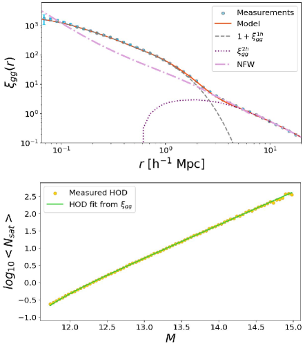
Figure 7: The top panel shows the correlation functions. The blue-filled circles (for which the error bars are small enough to be unnoticeable except on very small scales) are the measured correlation function using the real-space Cartesian coordinates of the Dark Sage  galaxies. The red solid curve is the model correlation function fit to the measurements using our new halo density profile for galaxies. The pink dash-dotted curve is the model correlation function calculated using the NFW profile and the yellow dots of the bottom panel. In the bottom panel, the green line is the HOD inferred from the fitted correlation function using our new profile model, the yellow dots are the measured HOD (errorbars are tiny). So our fitting method combined with the new profile model does an excellent job of recovering the true HOD from fitting only the correlation function. The fit results of the HOD parameters are displayed in Fig.10 of Appendix B.

Comparing the pink dash-dotted curve to the blue filled circles and red solid curve, we find that at larger scales $r>3\,h^{-1}$ Mpc, the model correlation function calculated using the NFW profile agrees with the measurements and the model predicted by Eq. 2, since this scale is dominated by the two-halo term, which is not sensitive to the galaxy number density profile of haloes. However, at smaller scales, i.e. $r<3\,h^{-1}$ Mpc, a galaxy number density profile of haloes different to NFW, such as the one developed in this work, is needed to correctly recover the correlation function. Particularly, at scales of $r<0.1\,h^{-1}$ Mpc, the model correlation function calculated from the NFW profile is too high compared to the measurements, as there are fewer galaxies situated in the halo center region (see the left-hand panel of Fig. 4 for an example illustration).At scales of $r\in[0.1,~{}3]h^{-1}$ Mpc, the model correlation function calculated from the NFW profile is too low compared to the measurements, as satellite galaxies tend to be situated farther in the outskirts of the halo than the NFW profile predicts.In the bottom-left panel of Fig. 7, the green line is the HOD inferred from the fitted correlation function (red solid curve), which is in excellent agreement with the measured HOD. The fit results of the HOD parameters are displayed in the right-hand panels.

To summarise, in this section, we have proven that the galaxy number density profile of haloes Eq. 2, 5 and 6 can accurately reproduce the HOD and correlation function of Dark Sage galaxies.

5 Validating the galaxy number density profile of haloes using SDSS galaxies

5.1 Comparing the galaxy number density profile model of haloes to the measurements from SDSS galaxies

In Fig. 3, the red pentagrams show the $\alpha$ and $\beta$ values against halo mass $M$, obtain by comparing Eq. 2 to the measurements of real SDSS galaxies in halo mass bins. The halo mass bin width is around 0.06. The $\alpha$ values estimated from the SDSS galaxies are systematically lower than the values estimated from Dark Sage (blue dots), while the $\beta$ values estimated from the SDSS galaxies are systematically higher than Dark Sage (blue dots). However, the functional forms of Eq. 5 and 6 can still be used to model the red pentagrams (with different coefficients). Due to limited measurements in lower halo mass bins, the SDSS points become too noisy to infer anything concrete about their distributions. As such, we do not fit the them using Eq. 5 and 6. In future work, we aim to further test this using larger galaxies surveys such as WALLABY and DESI.

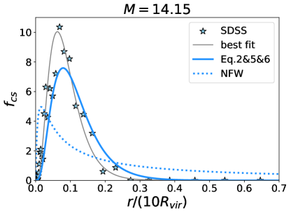
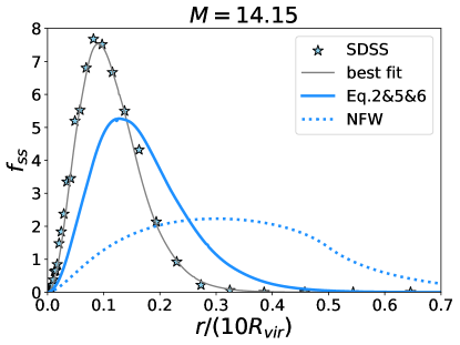
Figure 8: Comparing the $f_{cs}$ and $f_{ss}$ of SDSS galaxies to those of Dark Sage and NFW profile, in an example halo mass bin $M=14.15$.

In Fig. 8, the blue filled pentagrams in the top panel show the measured $f_{cs}$ in an example halo mass bin $M=14.15$. The grey curve is the model Eq. 2 fitting $\alpha$ and $\beta$ to the blue filled circles. The dashed-blue curve is the prediction from the NFW profile, which does not agree with the measured points. The solid-blue curve is the prediction of the new model for $M=14.15$ from Eq. 2, using the mass-dependent parameter values for $\alpha$ (Eq. 5) and $\beta$ (Eq. 6) (i.e. parameter values inferred from Dark Sage). Though it is slightly broader than the measurements, it is much better than the NFW profile (blue dashed curve) in matching the data (blue filled pentagrams). The discrepancy of Dark Sage  (the solid-blue curves) and SDSS (the blue filled pentagrams) could be caused by subhalo-finder issues in Millennium. The closer to the halo centre a subhalo is, the more likely a subhalo finder will fail to find it.

The blue filled pentagrams in the bottom panel of Fig. 8 show the measured $f_{ss}$ of SDSS galaxies, the grey curve is calculated the same as before, using the best fit values of $\alpha$ and $\beta$ ( i.e. the red stars in Fig. 3) into Eq. 9. The dashed-blue curve is the prediction from the NFW profile which is poorly agree with the measurement. The solid-blue curve is a prediction for $M=14.15$ from Eq. 9, using the mass-dependent parameter values for $\alpha$ (Eq. 5) and $\beta$ (Eq. 6).It is broader than the measurements, however it is a much better fit than the NFW profile to the blue filled pentagrams.

The minimum separation of the spectroscopic fibers of the telescope is 55 arcseconds (Tempel et al., 2014a), as for any smaller separation the fibers will collide. The distance limit of the sample of SDSS galaxies used in this paper is 330 Mpc $h^{-1}$ ($z<0.11$). Therefore, while the fiber collsions may lead to some incompleteness, this will bias the measurements for a separation of $r<0.088$ Mpc $h^{-1}$ at most. The halo mass range of the SDSS data used in this paper is $M\in[13.5,~{}14.8]$. Correspondingly, the range of virial radius is $R_{vir}\in[0.53,~{}1.35]$ Mpc $h^{-1}$. Therefore, using the SDSS data, the measurements of $f_{cs}$ (and $f_{ss}$) in $x<$0.0187 may not be reliable. However, this small-scale incompleteness is not expected to be a major problem. As illustrated by Fig.8, these measurements are located in the left-corner of the figure, and so they will not affect our fit too much.

Under the NFW profile, the satellite galaxies are much more close to the halo center, therefore, the gravitational potential and redshift calculated from the NFW profile are lower than the measurements, this will yeild incorrect measurements of correlation function odd-multi-pole, further more, bias the estimations of the cosmological parameters.

5.2 Galaxy two-point correlation function of SDSS galaxies

The top panel of Fig. 9 shows the HOD of satellite galaxies $N_{\rm sat}$ measured from the SDSS galaxies. After plugging $N_{\rm sat}$ and the galaxy number density profile model of haloes (Eqs 2, 5, 6) into Eq. 19, we show our model correlation function in the red solid curve of the bottom panel. We also plug $N_{\rm sat}$ and the NFW profile model into Eq. 19 to calculate the model correlation function, as shown in the pink dash-dotted curve of the bottom panel. The blue circles are the measurements from the SDSS galaxies.

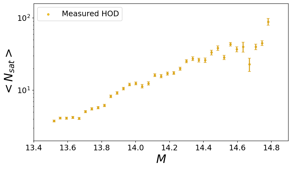
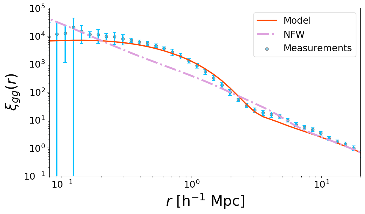
Figure 9: The top panels show the HOD of satellite galaxies measured from the SDSS galaxies. The bottom panel shows the galaxy two-point correlation functions $\xi_{gg}(r)$. The blue dots are the measurements from SDSS galaxies. The red solid curve is the model $\xi_{gg}(r)$ inferred from the measured HOD in the top panel and the halo density profile for galaxies Eq. 2, 5 and 6. The pink dash-dotted curve is the model $\xi_{gg}(r)$ inferred from the measured HOD in the top panel and the NFW profile.

Again, the correlation function predicted by our new galaxy number density profile of haloes is in much better agreement with the measurements (blue dots) than the NFW case. The discrepancy between our model and the data reflects the difference of the best-fitting $\alpha$ and $\beta$ values between Dark Sage and SDSS. The SDSS galaxies tend to be more concentrated to the halo center, therefore, the blue dots for small scales $r\leq 0.7\,h^{-1}$ Mpc are higher than the red curve, while the blue dots for intermediate scales $r\in[0.7,~{}3]h^{-1}$ Mpc are lower than the red curve.

As mentioned in the Section 5.1, due to the incompleteness from the fiber collision, the correlation function measurements below 0.088 Mpc $h^{-1}$ are not reliable. However, our analyse is mainly for $r>0.1$ Mpc $h^{-1}$ in Fig.9. Therefore, the incompleteness will not affect our findings.

6 Conclusion

In this paper, we have presented a new galaxy number density profile model of haloes (Eq. 2). The functional form of this model is determined using the Dark Sage semi-analytic model of galaxy formation. There are two free parameters ($\alpha,~{}\beta$) in the model. Based on the measurements from the Dark Sage simulation, we find that $\alpha$ and $\beta$ are relatively simple functions of halo mass $M$. We can use a linear function Eq. 5 to model the relation between $\alpha$ and $M$, and use a exponential function Eq. 6 to model the relation between $\beta$ and $M$. We also find that our galaxy number density profile model of haloes can correctly reproduce the galaxy two-point correlation function of the Dark Sage galaxies.

We derived the analytic expressions for the circular velocity and gravitational potential energy (see Eqs. 16 and 18) for the new model Eq. 2.

We also used the SDSS DR10 galaxy group catalogue to validate the galaxy number density profile of haloes and find that the functional form of our model (Eqs. 2, 5 and 6) is flexible enough to fit the data, although the best fit values of ($\alpha,~{}\beta$) are somewhat larger than the fit results from Dark Sage. The galaxies in the SDSS catalogue is more concentrated to the halo center compared to the galaxies of Dark Sage. The galaxy two-point correlation function predicted from our galaxy number density profile model of haloes is comparable to the measurement from SDSS galaxies.

The NFW density profile fails to model the radial distribution of satellite galaxies in their host halo for both the Dark Sage simulation and SDSS catalogue. And the NFW profile also fails to predict the two-point correlation functions for both the Dark Sage simulation and SDSS catalogue in small separation scales.

There are many extensions to this work that can be pursued in the future, including using larger galaxy group catalogues and simulations to further constrain $\alpha$ and $\beta$ at higher and lower halo masses, exploring the galaxy number density profile of haloes conditional on H i mass, testing our galaxy number density profile of haloes using emission line galaxies, and investigating how the galaxy number density profile of haloes affects the measurements of odd-multipoles of the correlation function.

Appendix A NFW Halo Density Profile

The Navarro–Frenk–White (NFW) profile (Navarro et al., 1996, 1997)

$$\rho_{m}(R)=\frac{\rho_{s}}{(R/R_{s})(1+R/R_{s})^{2}}~{},$$ (A1)

where

$$\rho_{s}=\frac{\rho_{0}\Delta}{3}\frac{c^{3}}{\ln(1+c)-c/(1+c)}~{},$$ (A2)

The $f_{ss}(x)$ for the NFW profile is given in the Appendix A of Zheng & Weinberg (2007), the expression is lengthy so not repeated here. The Fourier transformation of the NFW profile is expressed as (Cooray & Sheth, 2002)

$$\begin{split}y(k)&=\frac{1}{\ln(1+c)-c/(1+c)}\times\bigg{\{}-\frac{\sin(ckR_{s})}{(1+c)kR_{s}}\\ &+\sin(kR_{s})\left[SI([1+c]kR_{s})-SI(kR_{s})\right]\\ &+\cos(kR_{s})\left[CI([1+c]kR_{s})-CI(kR_{s})\right]\bigg{\}}~{},\end{split}$$ (A3)

where

$$SI(x)\equiv\int_{0}^{x}\frac{\sin t}{t}dt~{},CI(x)\equiv-\int_{x}^{\infty}\frac{\cos t}{t}dt~{},$$ (A4)

are the Trigonometric integrals. The mass interior to $r$ is given by (Sheth et al., 2001)

$$m(<r)=\frac{m_{\rm vir}}{R_{\rm vir}}\frac{r}{a[\ln(1+1/a)-1/(1+a)]}\left[\frac{\ln(1+x)}{x}-\frac{1}{1+x}\right]$$ (A5)

The circular velocity is (Sheth et al., 2001)

$$v^{2}_{c}=\frac{Gm_{\rm vir}}{R_{\rm vir}}\frac{1}{a[\ln(1+1/a)-1/(1+a)]}\left[\frac{\ln(1+x)}{x}-\frac{1}{1+x}\right]$$ (A6)

where $x=r/a$ and $a=1/c$. The gravitational potential energy is given by (Sheth et al., 2001)

$$\phi(r)=-\frac{Gm_{\rm vir}}{R_{\rm vir}}\frac{1}{a[\ln(1+1/a)-1/(1+a)]}\left[\frac{\ln(1+x)}{x}-\frac{a}{1+a}\right]$$ (A7)

Appendix B HOD parameters

Corresponding to Fig.7, the fit results of the HOD parameters in Eq.23 is shown in Fig.10.

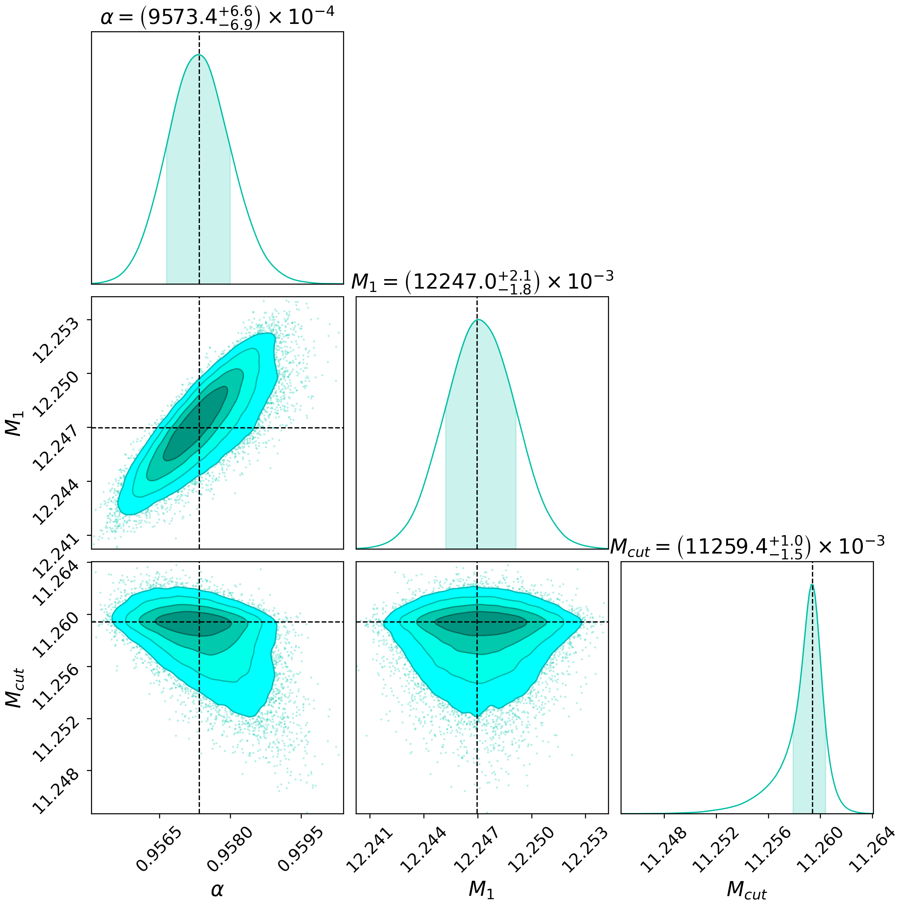
Figure 10: The fit results of the HOD parameters. The histograms display the distribution of out MCMC samples. The shaded areas in the 1D histograms indicate the 68% confidence level, while the 2D contours indicate the 1, 1.5, 2 and 2.5$\sigma$ regions.

References

- Ahn et al. (2014) Ahn, C. P., Alexandroff, R., Allende Prieto, C., et al. 2014, ApJS, 211, 17, doi: 10.1088/0067-0049/211/2/17
- Alam et al. (2020) Alam, S., Peacock, J. A., Kraljic, K., Ross, A. J., & Comparat, J. 2020, MNRAS, 497, 581, doi: 10.1093/mnras/staa1956
- Avila et al. (2020) Avila, S., Gonzalez-Perez, V., Mohammad, F. G., et al. 2020, MNRAS, 499, 5486, doi: 10.1093/mnras/staa2951
- Bartelmann (1996) Bartelmann, M. 1996, A&A, 313, 697, doi: 10.48550/arXiv.astro-ph/9602053
- Bell et al. (2003) Bell, E. F., Baugh, C. M., Cole, S., Frenk, C. S., & Lacey, C. G. 2003, MNRAS, 343, 367, doi: 10.1046/j.1365-8711.2003.06673.x
- Berlind & Weinberg (2002) Berlind, A. A., & Weinberg, D. H. 2002, ApJ, 575, 587, doi: 10.1086/341469
- Beutler et al. (2019) Beutler, F., Castorina, E., & Zhang, P. 2019, J. Cosmology Astropart. Phys, 2019, 040, doi: 10.1088/1475-7516/2019/03/040
- Bonvin (2014) Bonvin, C. 2014, Classical and Quantum Gravity, 31, 234002, doi: 10.1088/0264-9381/31/23/234002
- Brown et al. (2015) Brown, T., Catinella, B., Cortese, L., et al. 2015, MNRAS, 452, 2479, doi: 10.1093/mnras/stv1311
- Budzynski et al. (2012) Budzynski, J. M., Koposov, S. E., McCarthy, I. G., McGee, S. L., & Belokurov, V. 2012, MNRAS, 423, 104, doi: 10.1111/j.1365-2966.2012.20663.x
- Chaves-Montero et al. (2023) Chaves-Montero, J., Angulo, R. E., & Contreras, S. 2023, MNRAS, 521, 937, doi: 10.1093/mnras/stad243
- Chen & Afshordi (2023) Chen, A. Y., & Afshordi, N. 2023, Phys. Rev. D, 107, 103526, doi: 10.1103/PhysRevD.107.103526
- Chen et al. (2017) Chen, Y.-C., Ho, S., Mandelbaum, R., et al. 2017, MNRAS, 466, 1880, doi: 10.1093/mnras/stw3127
- Cole et al. (2000) Cole, S., Lacey, C. G., Baugh, C. M., & Frenk, C. S. 2000, MNRAS, 319, 168, doi: 10.1046/j.1365-8711.2000.03879.x
- Colless et al. (2001) Colless, M., Dalton, G., Maddox, S., et al. 2001, MNRAS, 328, 1039, doi: 10.1046/j.1365-8711.2001.04902.x
- Colless et al. (2003) Colless, M., Peterson, B. A., Jackson, C., et al. 2003, arXiv e-prints, astro, doi: 10.48550/arXiv.astro-ph/0306581
- Cooray & Sheth (2002) Cooray, A., & Sheth, R. 2002, Phys. Rep., 372, 1, doi: 10.1016/S0370-1573(02)00276-4
- Corwin et al. (1994) Corwin, Harold G., J., Buta, R. J., & de Vaucouleurs, G. 1994, AJ, 108, 2128, doi: 10.1086/117225
- DESI Collaboration et al. (2016) DESI Collaboration, Aghamousa, A., Aguilar, J., et al. 2016, arXiv e-prints, arXiv:1611.00036. https://arxiv.org/abs/1611.00036
- Di Dio & Seljak (2019) Di Dio, E., & Seljak, U. 2019, J. Cosmology Astropart. Phys, 2019, 050, doi: 10.1088/1475-7516/2019/04/050
- Fontanot et al. (2009) Fontanot, F., De Lucia, G., Monaco, P., Somerville, R. S., & Santini, P. 2009, MNRAS, 397, 1776, doi: 10.1111/j.1365-2966.2009.15058.x
- Foreman-Mackey et al. (2013) Foreman-Mackey, D., Hogg, D. W., Lang, D., & Goodman, J. 2013, PASP, 125, 306, doi: 10.1086/670067
- Gaztanaga et al. (2017) Gaztanaga, E., Bonvin, C., & Hui, L. 2017, J. Cosmology Astropart. Phys, 2017, 032, doi: 10.1088/1475-7516/2017/01/032
- Guo et al. (2014) Guo, H., Zheng, Z., Zehavi, I., et al. 2014, MNRAS, 441, 2398, doi: 10.1093/mnras/stu763
- Guo et al. (2015) —. 2015, MNRAS, 446, 578, doi: 10.1093/mnras/stu2120
- Hand et al. (2018) Hand, N., Feng, Y., Beutler, F., et al. 2018, AJ, 156, 160, doi: 10.3847/1538-3881/aadae0
- Hernquist (1990) Hernquist, L. 1990, ApJ, 356, 359, doi: 10.1086/168845
- Hinton (2016) Hinton, S. R. 2016, The Journal of Open Source Software, 1, 00045, doi: 10.21105/joss.00045
- Howlett et al. (2015) Howlett, C., Ross, A. J., Samushia, L., Percival, W. J., & Manera, M. 2015, MNRAS, 449, 848, doi: 10.1093/mnras/stu2693
- Howlett et al. (2022) Howlett, C., Said, K., Lucey, J. R., et al. 2022, MNRAS, 515, 953, doi: 10.1093/mnras/stac1681
- Huchra et al. (2012) Huchra, J. P., Macri, L. M., Masters, K. L., et al. 2012, ApJS, 199, 26, doi: 10.1088/0067-0049/199/2/26
- Hunter (2007) Hunter, J. D. 2007, Computing in Science Engineering, 9, 90, doi: 10.1109/MCSE.2007.55
- Jarrett et al. (2003) Jarrett, T. H., Chester, T., Cutri, R., Schneider, S. E., & Huchra, J. P. 2003, AJ, 125, 525, doi: 10.1086/345794
- Kaiser (1987) Kaiser, N. 1987, MNRAS, 227, 1, doi: 10.1093/mnras/227.1.1
- Keeton (2001) Keeton, C. R. 2001, arXiv e-prints, astro, doi: 10.48550/arXiv.astro-ph/0102341
- Koribalski et al. (2020) Koribalski, B. S., Staveley-Smith, L., Westmeier, T., et al. 2020, Ap&SS, 365, 118, doi: 10.1007/s10509-020-03831-4
- Kraljic et al. (2018) Kraljic, K., Arnouts, S., Pichon, C., et al. 2018, MNRAS, 474, 547, doi: 10.1093/mnras/stx2638
- Kravtsov et al. (1998) Kravtsov, A. V., Klypin, A. A., Bullock, J. S., & Primack, J. R. 1998, ApJ, 502, 48, doi: 10.1086/305884
- Lacey & Cole (1993) Lacey, C., & Cole, S. 1993, MNRAS, 262, 627, doi: 10.1093/mnras/262.3.627
- Leauthaud et al. (2017) Leauthaud, A., Saito, S., Hilbert, S., et al. 2017, MNRAS, 467, 3024, doi: 10.1093/mnras/stx258
- Lewis et al. (2000) Lewis, A., Challinor, A., & Lasenby, A. 2000, Astrophys. J., 538, 473, doi: 10.1086/309179
- Li et al. (2014) Li, R., Shan, H., Mo, H., et al. 2014, MNRAS, 438, 2864, doi: 10.1093/mnras/stt2395
- Łokas & Mamon (2001) Łokas, E. L., & Mamon, G. A. 2001, MNRAS, 321, 155, doi: 10.1046/j.1365-8711.2001.04007.x
- Maller & Bullock (2004) Maller, A. H., & Bullock, J. S. 2004, MNRAS, 355, 694, doi: 10.1111/j.1365-2966.2004.08349.x
- Martin et al. (2010) Martin, A. M., Papastergis, E., Giovanelli, R., et al. 2010, ApJ, 723, 1359, doi: 10.1088/0004-637X/723/2/1359
- McDonald (2009) McDonald, P. 2009, J. Cosmology Astropart. Phys, 2009, 026, doi: 10.1088/1475-7516/2009/11/026
- Moore (1994) Moore, B. 1994, Nature, 370, 629, doi: 10.1038/370629a0
- Moore et al. (1999) Moore, B., Quinn, T., Governato, F., Stadel, J., & Lake, G. 1999, MNRAS, 310, 1147, doi: 10.1046/j.1365-8711.1999.03039.x
- Navarro et al. (1996) Navarro, J. F., Frenk, C. S., & White, S. D. M. 1996, ApJ, 462, 563, doi: 10.1086/177173
- Navarro et al. (1997) Navarro, J. F., Frenk, C. S., & White, S. D. M. 1997, ApJ, 490, 493, doi: 10.1086/304888
- Nishimichi et al. (2019) Nishimichi, T., Takada, M., Takahashi, R., et al. 2019, ApJ, 884, 29, doi: 10.3847/1538-4357/ab3719
- O’Brien et al. (2010) O’Brien, J. C., Freeman, K. C., & van der Kruit, P. C. 2010, A&A, 515, A63, doi: 10.1051/0004-6361/200912568
- Orsi & Angulo (2018) Orsi, Á. A., & Angulo, R. E. 2018, MNRAS, 475, 2530, doi: 10.1093/mnras/stx3349
- Padmanabhan et al. (2017) Padmanabhan, H., Refregier, A., & Amara, A. 2017, MNRAS, 469, 2323, doi: 10.1093/mnras/stx979
- Paranjape et al. (2021) Paranjape, A., Choudhury, T. R., & Sheth, R. K. 2021, MNRAS, 503, 4147, doi: 10.1093/mnras/stab722
- Pillepich et al. (2018) Pillepich, A., Springel, V., Nelson, D., et al. 2018, MNRAS, 473, 4077, doi: 10.1093/mnras/stx2656
- Qin et al. (2019) Qin, F., Howlett, C., & Staveley-Smith, L. 2019, MNRAS, 487, 5235, doi: 10.1093/mnras/stz1576
- Qin et al. (2022) Qin, F., Howlett, C., Stevens, A. R. H., & Parkinson, D. 2022, ApJ, 937, 113, doi: 10.3847/1538-4357/ac8b6f
- Qin et al. (2021) Qin, F., Parkinson, D., Howlett, C., & Said, K. 2021, ApJ, 922, 59, doi: 10.3847/1538-4357/ac249d
- Rocher et al. (2023) Rocher, A., Ruhlmann-Kleider, V., Burtin, E., et al. 2023, arXiv e-prints, arXiv:2306.06319, doi: 10.48550/arXiv.2306.06319
- Sheth et al. (2001) Sheth, R. K., Hui, L., Diaferio, A., & Scoccimarro, R. 2001, MNRAS, 325, 1288, doi: 10.1046/j.1365-8711.2001.04222.x
- Sinha & Garrison (2020) Sinha, M., & Garrison, L. H. 2020, MNRAS, 491, 3022, doi: 10.1093/mnras/stz3157
- Spergel et al. (2003) Spergel, D. N., Verde, L., Peiris, H. V., et al. 2003, ApJS, 148, 175, doi: 10.1086/377226
- Springel et al. (2005) Springel, V., White, S. D. M., Jenkins, A., et al. 2005, Nature, 435, 629, doi: 10.1038/nature03597
- Square Kilometre Array Cosmology Science Working Group et al. (2020) Square Kilometre Array Cosmology Science Working Group, Bacon, D. J., Battye, R. A., et al. 2020, PASA, 37, e007, doi: 10.1017/pasa.2019.51
- Stevens et al. (2016) Stevens, A. R. H., Croton, D. J., & Mutch, S. J. 2016, MNRAS, 461, 859, doi: 10.1093/mnras/stw1332
- Stevens et al. (2017) Stevens, A. R. H., Croton, D. J., Mutch, S. J., & Sinha, M. 2017, Dark Sage: Semi-analytic model of galaxy evolution. http://ascl.net/1706.004
- Stevens et al. (2018) Stevens, A. R. H., Lagos, C. d. P., Obreschkow, D., & Sinha, M. 2018, MNRAS, 481, 5543, doi: 10.1093/mnras/sty2650
- Tempel et al. (2014a) Tempel, E., Tamm, A., Gramann, M., et al. 2014a, A&A, 566, A1, doi: 10.1051/0004-6361/201423585
- Tempel et al. (2014b) —. 2014b, Flux- and volume-limited groups for SDSS galaxies, Version 06-Aug-2019 (last modified), Centre de Donnees astronomique de Strasbourg (CDS), doi: https://doi.org/10.26093/cds/vizier.35660001
- Tinker et al. (2005) Tinker, J. L., Weinberg, D. H., Zheng, Z., & Zehavi, I. 2005, ApJ, 631, 41, doi: 10.1086/432084
- Virtanen et al. (2020) Virtanen, P., Gommers, R., Oliphant, T. E., et al. 2020, Nature Methods, 17, 261, doi: 10.1038/s41592-019-0686-2
- Wang et al. (2022) Wang, J., Yang, X., Zhang, J., et al. 2022, ApJ, 936, 161, doi: 10.3847/1538-4357/ac8986
- Wetzel et al. (2013) Wetzel, A. R., Tinker, J. L., Conroy, C., & van den Bosch, F. C. 2013, MNRAS, 432, 336, doi: 10.1093/mnras/stt469
- White & Rees (1978) White, S. D. M., & Rees, M. J. 1978, MNRAS, 183, 341, doi: 10.1093/mnras/183.3.341
- Yang et al. (2003) Yang, X., Mo, H. J., & van den Bosch, F. C. 2003, MNRAS, 339, 1057, doi: 10.1046/j.1365-8711.2003.06254.x
- Yang et al. (2013) Yang, X., Mo, H. J., van den Bosch, F. C., et al. 2013, ApJ, 770, 115, doi: 10.1088/0004-637X/770/2/115
- York et al. (2000) York, D. G., Adelman, J., Anderson, John E., J., et al. 2000, AJ, 120, 1579, doi: 10.1086/301513
- Yuan et al. (2023) Yuan, S., Zhang, H., Ross, A. J., et al. 2023, arXiv e-prints, arXiv:2306.06314, doi: 10.48550/arXiv.2306.06314
- Zheng (2004) Zheng, Z. 2004, ApJ, 610, 61, doi: 10.1086/421542
- Zheng et al. (2007) Zheng, Z., Coil, A. L., & Zehavi, I. 2007, ApJ, 667, 760, doi: 10.1086/521074
- Zheng & Guo (2016) Zheng, Z., & Guo, H. 2016, MNRAS, 458, 4015, doi: 10.1093/mnras/stw523
- Zheng & Weinberg (2007) Zheng, Z., & Weinberg, D. H. 2007, ApJ, 659, 1, doi: 10.1086/512151
- Zwaan et al. (2005) Zwaan, M. A., Meyer, M. J., Staveley-Smith, L., & Webster, R. L. 2005, MNRAS, 359, L30, doi: 10.1111/j.1745-3933.2005.00029.x