The Levin approach to the numerical calculation of phase functions

Abstract

When the eigenvalues of the coefficient matrix for a linear scalar ordinary differential equation are of large magnitude, its solutions exhibit complicated behaviour, such as high-frequency oscillations, rapid growth or rapid decay. The cost of representing such solutions using standard techniques typically grows with the magnitudes of the eigenvalues. As a consequence, the running times of standard solvers for ordinary differential equations also grow with these eigenvalues. It is well known, however, that a large class of scalar ordinary differential equations with slowly-varying coefficients admit slowly-varying phase functions that can be represented efficiently, regardless of the magnitudes of the eigenvalues of the corresponding coefficient matrix. Here, we introduce two numerical algorithms for constructing slowly-varying phase functions for linear scalar ordinary differential equations inspired by the classical Levin method for evaluating oscillatory integrals. The running times of our algorithms depend on the complexity of an equation’s coefficients, but are largely independent of the magnitudes of the eigenvalues of its coefficient matrix. Once these phase functions have been constructed, essentially any reasonable initial or boundary value problem for the scalar equation can be easily solved, essentially instantaneously. The results of extensive numerical experiments demonstrating the properties of our algorithms are presented.

1 Introduction

The cost to represent the solutions of an $n^{th}$ order linear homogeneous ordinary differential equation

$$y^{(n)}(t)+q_{n-1}(t)y^{(n-1)}(t)+\cdots+q_{1}(t)y^{\prime}(t)+q_{0}(t)y(t)=0$$ (1)

using standard techniques, such as polynomial or trigonometric expansions, increases with the magnitudes of the eigenvalues $\lambda_{1}(t),\ldots,\lambda_{n}(t)$ of the coefficient matrix

$$A(t)=\left(\begin{array}[]{cccccccc}0&1&0&\cdots&0&0\\ 0&0&1&\cdots&0&0\\ \vdots&&&\ddots&&\vdots\\ 0&0&0&\cdots&1&0\\ 0&0&0&\cdots&0&1\\ -q_{0}(t)&-q_{1}(t)&-q_{2}(t)&\cdots&-q_{n-2}(t)&-q_{n-1}(t)\\ \end{array}\right)$$ (2)

obtained from (1) in the usual way. As a consequence, when conventional solvers for ordinary differential equations are applied to equations of this form, their running times also increase with the magnitudes of the eigenvalues of (2).

It is well known, however, that many such equations admit phase functions whose cost to represent via standard methods depends on the complexity of the coefficients $q_{0},\ldots,q_{n-1}$, but not the magnitudes of the eigenvalues of (2). Indeed, if the $q_{0},\ldots,q_{n-1}$ are slowly-varying on an interval $I$ and the coefficient matrix (2) corresponding to (1) has eigenvalues $\lambda_{1}(t),\ldots,\lambda_{n}(t)$ which are distinct for all $t$ in $I$, then it is possible to find slowly-varying functions $\psi_{1},\ldots,\psi_{n}\colon I\to\mathbb{C}$ such that

$$\left\{\exp\left(\psi_{j}(t)\right):j=1,\ldots,n\right\}$$ (3)

is a basis for the space of solutions of (1) given on the interval $I$. This observation is the foundation of the WKB method, as well as many other techniques for the asymptotic analysis of ordinary differential equations (see, for instance, Miller , Wasov and SpiglerPhase1 ; SpiglerPhase2 ; SpiglerZeros ).

An equation of the form (1) is said to be nondegenerate on the interval $I$ provided the above condition holds; that is, if all of the eigenvalues $\lambda_{1}(t),\ldots,\lambda_{n}(t)$ of the corresponding coefficient matrix (2) are distinct for each $t\in I$. Moreover, $t_{0}$ is a turning point for (1) if the eigenvalues of (2) are distinct in a deleted neighbourhood of $t_{0}$ but coalesce at $t_{0}$. The derivatives of the phase functions $\psi_{1},\ldots,\psi_{n}$, which we will denote by $r_{1},\ldots,r_{n}$, satisfy an $(n-1)^{st}$ order nonlinear inhomogeneous ordinary differential equation, the general form of which is quite complicated. When $n=2$, it is the Riccati equation

$$r^{\prime}(t)+(r(t))^{2}+q_{1}(t)r(t)+q_{0}(t)=0;$$ (4)

when $n=3$, the nonlinear equation is

$$r^{\prime\prime}(t)+3r^{\prime}(t)r(t)+(r(t))^{3}+q_{2}(t)r^{\prime}(t)+q_{2}(t)(r(t))^{2}+q_{1}(t)r(t)+q_{0}(t)=0;$$ (5)

and, for $n=4$, we have

$$r^{\prime\prime\prime}(t) +4r^{\prime\prime}(t)r(t)+3(r^{\prime}(t))^{2}+6r^{\prime}(t)(r(t))^{2}+(r(t))^{4}+q_{3}(t)(r(t))^{3}+q_{3}(t)r^{\prime\prime}(t)+3q_{3}(t)r^{\prime}(t)r(t)$$ (6)

$$+q_{2}(t)(r(t))^{2}+q_{2}(t)r^{\prime}(t)+q_{1}(t)r(t)+q_{0}(t)=0.$$

By a slight abuse of terminology, we will refer to the $(n-1)^{st}$ order nonlinear equation obtained by inserting the representation

$$y(t)=\exp\left(\int r(t)\,dt\right)$$ (7)

into (1) as the $(n-1)^{st}$ order Riccati equation, or, alternatively, the Riccati equation for (1).

An obvious approach to initial and boundary value boundary problems for (1) calls for constructing a suitable collection of slowly-varying phase functions by solving the corresponding Riccati equation numerically. Doing so is not as straightforward as it sounds, however. The principal difficulty is that most solutions of the Riccati equation for (1) are rapidly-varying when the eigenvalues $\lambda_{1}(t),\ldots,\lambda_{n}(t)$ are of large magnitude, and some mechanism is needed to select the slowly-varying solutions.

The article BremerPhase introduces such a technique for the case of second order linear ordinary differential equations, all of which can be put in the form

$$y^{\prime\prime}(t)+q(t)y(t)=0.$$ (8)

The eigenvalues of the corresponding coefficient matrix (2) are given by

$$\lambda_{1}(t)=\sqrt{-q(t)}\ \ \ \mbox{and}\ \ \ \lambda_{2}(t)=-\sqrt{-q(t)}.$$ (9)

In particular, (8) is nondegenerate on any interval on which $q$ does not vanish, and $t_{0}$ is a turning point if and only if $q$ has an isolated zero there. The algorithm of BremerPhase can only be applied on intervals $I$ on which (8) is nondegenerate. It uses a continuation scheme of sorts to compute the values of the derivatives $r_{1}$ and $r_{2}$ of the desired slowly-varying phase functions $\psi_{1}$ and $\psi_{2}$ at a particular point $c$ in $I$. The Riccati equation is then solved using $r_{1}(c)$ and $r_{2}(c)$ as initial conditions in order to calculate $r_{1}$ and $r_{2}$ over the whole interval. The slowly-varying phase functions are obtained by integration.

A simple modification of the algorithm of BremerPhase , described in BremerPhase2 , extends it to the case in which $q$ is nonzero on an interval $[a,b]$, except at a finite number of isolated zeros; that is, when (8) is nondegenerate over $[a,b$] with a finite number of turning points. The algorithm operates by introducing a partition $a=\xi_{1}<\xi_{2}<\ldots<\xi_{k}=b$ of $[a,b]$ such that $\xi_{2},\ldots,\xi_{k-1}$ are the roots of $q$ in the open interval $(a,b)$. Then, for each $j=1,\ldots,k-1$, the algorithm constructs two slowly-varying phase functions $\psi_{1}^{j}$ and $\psi_{2}^{j}$ such that

$$\exp\left(\psi_{1}^{j}(t)\right)\ \ \ \mbox{and}\ \ \ \exp\left(\psi_{2}^{j}(t)\right)$$ (10)

comprise a basis in the space of solutions of (8) given on the interval $\left[\xi_{j},\xi_{j+1}\right]$ using the approach of BremerPhase . It is necessary to partition $[a,b]$ because slowly-varying phase functions cannot always be extended across a turning point. It is relatively straightforward to generalize the method of BremerPhase ; BremerPhase2 to higher order scalar equations. However, that is not the approach we take in this article. The authors have found that while the resulting algorithm is highly-effective in the case of a large collection of equations of the form (1), it has properties very similar to another approach discussed in this paper, but with slightly inferior performance.

In this article, we describe two methods for constructing a collection $\psi_{1},\ldots,\psi_{n}$ of slowly-varying phase functions such that (3) is a basis in the space of solutions of (1). Both are inspired by the classical Levin approach to the numerical evaluation of oscillatory integrals. Introduced in Levin , the Levin method is based on the observation that inhomogeneous equations of the form

$$y^{\prime}(t)+p_{0}(t)y(t)=f(t)$$ (11)

admit solutions whose complexity depends on that of $p_{0}$ and $f$, but not on the magnitude of $p_{0}$. This principle extends to the case of equations of the form

$$y^{(n)}(t)+p_{n-1}(t)y^{(n-1)}(t)+\cdots+p_{1}(t)y^{\prime}(y)+p_{0}(t)y(t)=f(t).$$ (12)

That is, such equations admit solutions whose complexity depends on that of the right-hand side $f$ and of the coefficients $p_{0},\ldots,p_{n-1}$, but not on the magnitudes of the $p_{0},\ldots,p_{n-1}$. We exploit this principle by applying Newton’s method to the Riccati equation for (1). Starting with a slowly-varying initial guess ensures that each of linearized equations which arise are of the form (12), and so admit a slowly-varying solution. Consequently, a slowly-varying solution of the Riccati equation can be constructed via Newton’s method as long as an appropriate slowly-varying initial guess is known. Conveniently enough, there is an obvious mechanism for generating $n$ slowly-varying initial guesses for the solution of the $(n-1)^{st}$ order Riccati equation. In particular, the eigenvalues $\lambda_{1}(t),\ldots,\lambda_{n}(t)$ of the matrix (2), which are often used as low-accuracy approximations of solutions of the Riccati equation in asymptotic methods, are suitable as initial guesses for the Newton procedure.

Complicating matters is the fact that the differential operator

$$D\left[y\right](t)=y^{(n)}(t)+p_{n-1}(t)y^{(n-1)}(t)+\cdots+p_{1}(t)y^{\prime}(y)+p_{0}(t)y(t)$$ (13)

appearing on the left-hand side of (12) admits a nontrivial nullspace comprising all solutions of the homogeneous equation

$$y^{(n)}(t)+p_{n-1}(t)y^{(n-1)}(t)+\cdots+p_{1}(t)y^{\prime}(y)+p_{0}(t)y(t)=0.$$ (14)

This means, of course, that (12) is not uniquely solvable. But it also implies that most solutions of (12) are rapidly-varying when the coefficients $p_{0},\ldots,p_{n-1}$ are of large magnitude since the homogeneous equation (14) admits rapidly-varying solutions in such cases. It is observed in Levin that when the solutions of (14) are all rapidly-varying but (12) admits a slowly-varying solution $y_{0}$, a simple spectral collocation method can be used to compute $y_{0}$ provided some care is taken in choosing the discretization grid. In particular, if the collocation grid is sufficient to resolve the slowly-varying solution $y_{0}$, but not the solutions of (14), then the matrix discretizing (13) will be well-conditioned and inverting it will yield $y_{0}$.

We refer to the first of the algorithms introduced here as the global Levin method. It operates by subdividing $[a,b]$ until, on each resulting subinterval, every one of the slowly-varying phase functions $\psi_{1},\ldots,\psi_{n}$ it constructs is accurately represented by a Chebyshev expansion of a fixed order. The derivatives $r_{1},\ldots,r_{n}$ of the phase functions $\psi_{1},\ldots,\psi_{n}$ are calculated on each subinterval by applying Newton’s method to the Riccati equation and solving the resulting linearized equations via a spectral collocation method. The method is highly accurate and effective, as long as the eigenvalues $\lambda_{1}(t),\ldots,\lambda_{n}(t)$ of the coefficient matrix (2) are of large magnitude on the entire interval $[a,b]$. In this case, each slowly-varying solution of the Riccati equation is isolated from the others so that the linear operators which arise during the Newton procedure have no slowly-varying elements in their nullspaces. Consequently, the spectral collocation method used to solve the linearized equations always yields a unique solution and the Newton iterates converge with no difficulty to a slowly-varying phase function.

When one or more of the eigenvalues $\lambda_{j}(t)$ is of small magnitude on some part of $[a,b]$, the global Levin method can fail. In this event, there are multiple slowly-varying solution of the Riccati equation near each initial guess. Accordingly, the Newton iterates can converge to different slowly-varying solutions of the Riccati equation, and because the global Levin method is an adaptive approach which subdivides the interval $[a,b]$, it can obtain different solutions on different subintervals. In particular, the functions obtained from the global Levin method in such cases can be discontinuous across the boundaries of the discretization subintervals, even though they locally satisfy the Riccati equation on each particular subinterval (this effect can clearly be seen in Figure 14 of Subsection 5.6.)

The second algorithm of this paper, which we call the local Levin method, is usually slower and slightly less accurate than the global Levin method in cases in which both apply, but it overcomes the difficulties which arise when the coefficient matrix (2) admits eigenvalues of small magnitude. The local method operates in a manner very similar to the algorithm of BremerPhase — it first computes the values of the derivatives $r_{1},r_{2},\ldots,r_{n}$ of the desired slowly-varying phase functions $\psi_{1},\ldots,\psi_{n}$ at a point $c$ and then solves the Riccati equation numerically with those values used as initial conditions in order to construct $r_{1},r_{2},\ldots,r_{n}$ over the whole interval $[a,b]$. Rather than the continuation method of BremerPhase , however, the values of the $r_{1},r_{2},\ldots,r_{n}$ at $c$ are computed by applying the Levin approach to a single small subinterval of $[a,b]$ containing $c$. Because the Levin approach is only used on a single subinterval of $[a,b]$, the nonuniqueness of the slowly-varying phase functions is no longer a concern — any set of slowly-varying phase functions suffices for our purposes. For the sake of simplicity, we describe the local Levin method in the case in which (1) is nondegenerate on the entire interval $[a,b]$ of interest. However, it can easily be extended to equations of the form (1) that are nondegenerate on $[a,b]$ except at a finite number of turning points by partitioning $[a,b]$ and applying it on each of the resulting subintervals in the manner of BremerPhase2 .

Our algorithms bear some superficial similarities to Magnus expansion methods, which are another class of numerical solvers for systems of ordinary differential equations that rely on the exponential representation of solutions. Introduced in Magnus , Magnus expansions are certain series of the form

$$\sum_{k=1}^{\infty}\Omega_{k}(t)$$ (15)

such that $\exp\left(\sum_{k=1}^{\infty}\Omega_{k}(t)\right)$ locally represents a fundamental matrix for a system of differential equations

$$\mathbf{y}^{\prime}(t)=A(t)\mathbf{y}(t).$$ (16)

The first few terms for the series around $t=0$ are given by

$$\Omega_{1}(t) =\int_{0}^{t}A(s)\ ds,$$ (17)

$$\Omega_{2}(t) =\frac{1}{2}\int_{0}^{t}\int_{0}^{t_{1}}\left[A(t_{1}),A(t_{2})\right]\,dt_{2}dt_{1}\ \ \ \mbox{and}$$

$$\Omega_{3}(t) =\frac{1}{6}\int_{0}^{t}\int_{0}^{t_{1}}\int_{0}^{t_{2}}\left[A(t_{1}),\left[A(t_{2}),A(t_{3})\right]\right]+\left[A(t_{3}),\left[A(t_{2}),A(t_{1})\right]\right]\,dt_{3}dt_{2}dt_{1}.$$

The straightforward evaluation of the $\Omega_{j}$ is nightmarishly expensive; however, a clever technique which renders the calculations manageable is introduced in Iserles101 and it paved the way for the development of a class of numerical solvers which represent a fundamental matrix for (16) over an interval $I$ via a collection of truncated Magnus expansions. While the entries of the $\Omega_{j}$ are slowly-varying whenever the entries of $A(t)$ are slowly-varying, the radius of convergence of the series in (15) depends on the magnitude of the coefficient matrix $A(t)$, which is, in turn, related to the magnitudes of the eigenvalues of $A(t)$. Of course, this means that the number of Magnus expansions which are needed, and hence the cost of the method, depends on the magnitudes of the eigenvalues of $A(t)$. See, for instance, Iserles102 which gives for estimates of the growth in the running time of Magnus expansion methods in the case of an equation of the form (8) as a function of the magnitude of the coefficient $q$.

The algorithms of this paper, by contrast, represent a fundamental matrix for (16) with $A(t)$ given by (2) in the form

$$\exp\left(\begin{array}[]{ccccc}\psi_{1}(t)&&&&\\ &\psi_{2}(t)&&&\\ &&\ddots&&\\ &&&\psi_{n}(t)&\\ \end{array}\right),$$ (18)

where each $\psi_{j}$ is slowly-varying and can be represented at a cost independent of the magnitudes of the eigenvalues of $A(t)$. Interestingly, as a consequence of standard uniqueness results for ordinary differential equations, in the case in which $A(t)$ is of the scalar form (2) and $\psi_{1}(0)=\psi_{2}(0)=\cdots=\psi_{n}(0)=1$, the Magnus expansion

$$\exp\left(\sum_{k=1}^{\infty}\Omega_{k}(t)\right)$$ (19)

for (16) around $t=0$ must converge to (18). It follows that

$$\sum_{k=1}^{\infty}\Omega_{k}(t)$$ (20)

is the sum of the diagonal matrix whose nonzero entries are $\psi_{1}(t),\ldots,\psi_{n}(t)$ and a logarithm of the identity matrix. In particular, Magnus expansions converge to a matrix which can be represented at a cost independent of the magnitudes even though the individual terms in the expansion do not have this property.

Ostensibly, Magnus expansion methods apply to a much large class of systems of differential equations than the algorithms we describe here. However, since essentially any system of ordinary differential equations can be converted into scalar form (see, for instance, Kolchin ), it is possible to use our methods to solve a large class of systems of linear ordinary differential equations in time independent of the magnitudes of their coefficient matrices. We give one such example in the numerical experiments of this paper (see Section 5.7) and leave a description of this approach to a future work. We note, however, that an approach of this type involves representing a fundamental matrix for a system of differential equations (16) in the form

$$\Phi(t)\exp\left(\begin{array}[]{ccccc}\psi_{1}(t)&&&&\\ &\psi_{2}(t)&&&\\ &&\ddots&&\\ &&&\psi_{n}(t)&\\ \end{array}\right),$$ (21)

where $\Phi$ is an appropriately chosen slowly-varying transformation matrix and the $\psi_{1}(t),\ldots,\psi_{n}(t)$ are slowly-varying phase functions for a scalar equation.

The remainder of this article is organized as follows. In Section 2 we detail the procedure used by the local and global Levin method to construct the derivatives of the slowly-varying phase functions over a single subinterval of the interval $[a,b]$ over which (1) is given. A description of the global Levin method appears in Section 3, while Section 4 details the local Levin method. The results of numerical experiments demonstrating the properties of these algorithms are discussed in Section 5. We comment on the algorithms of this article and give a few brief suggestions for future work in Section 6. Appendix A details a standard adaptive spectral solver for ordinary differential equations which is used by the local Levin method, and to construct reference solutions in our numerical experiments.

2 The Levin procedure for a single subinterval

In this section, we describe the procedure used by the local and global Levin methods to construct phase functions on a single subinterval $[c,d]$ of the domain $[a,b]$ over which the equation (1) is given. The procedure takes as input the following:

1. the subinterval $[c,d]$;

2. an external subroutine for evaluating the coefficients $q_{0},\ldots,q_{n-1}$ in (1); and

3. an integer $k$ which controls the order of the Chebyshev expansions used to represent phase functions over $[c,d]$.

For each $j=1,\ldots,n$, it outputs a $(k-1)^{st}$ order Chebyshev expansion which represents the derivative $r_{j}$ of the phase function $\psi_{j}$ over the interval $[c,d]$. The procedure operates as follows:

1. Construct the $k$-point extremal Chebyshev grid $t_{1},\ldots,t_{k}$ on the interval $[c,d]$ and the corresponding $k\times k$ Chebyshev spectral differentiation matrix $D$. The nodes are given by the formula

   $$t_{j}=\frac{d-c}{2}\cos\left(\pi\frac{n-j}{n-1}\right)+\frac{d+c}{2}.$$ (22)

   The matrix $D$ takes the vector of values

   $$\left(\begin{array}[]{c}f(t_{1})\\ f(t_{2})\\ \vdots\\ f(t_{k})\\ \end{array}\right)$$ (23)

   of a Chebyshev expansion of the form

   $$f(t)=\sum_{j=0}^{k-1}a_{j}T_{j}\left(\frac{2}{d-c}t+\frac{d+c}{d-c}\right)$$ (24)

   to the vector

   $$\left(\begin{array}[]{c}f^{\prime}(t_{1})\\ f^{\prime}(t_{2})\\ \vdots\\ f^{\prime}(t_{k})\\ \end{array}\right)$$ (25)

   of the values of its derivatives at the nodes $t_{1},\ldots,t_{j}$.

2. Evaluate the coefficients $q_{0},\ldots,q_{n-1}$ at the points $t_{1},\ldots,t_{n}$ by calling the external subroutine supplied by the user.

3. Calculate the values of $n$ initial guesses $r_{1},\ldots,r_{n}$ for the Newton procedure at the nodes $t_{1},\ldots,t_{n}$ by computing the eigenvalues of the coefficient matrices

   $$A_{j}=\left(\begin{array}[]{cccccccc}0&1&0&\cdots&0&0\\ 0&0&1&\cdots&0&0\\ \vdots&&&\ddots&&\vdots\\ 0&0&0&\cdots&1&0\\ 0&0&0&\cdots&0&1\\ -q_{0}(t_{j})&-q_{1}(t_{j})&-q_{2}(t_{j})&\cdots&-q_{n-2}(t_{j})&-q_{n-1}(t_{j})\\ \end{array}\right),\ \ \ j=1,\ldots,k.$$ (26)

   More explicitly, the eigenvalues of $A_{j}$ give the values of $r_{1}(t_{j}),\ldots,r_{n}(t_{j})$.

4. Perform Newton iterations in order to refine each of the initial guesses $r_{1},\ldots,r_{n}$. Because the general form of the Riccati equation is quite complicated, we illustrate the procedure when $n=2$, in which case the Riccati equation is simply

   $$r^{\prime}(t)+(r(t))^{2}+q_{1}(t)r(t)+q_{0}(t)=0.$$ (27)

   In each iteration, we perform the following steps:

   1. Compute the residual

      $$\xi(t)=r^{\prime}(t)+(r(t))^{2}+q_{1}(t)r(t)+q_{0}(t)$$ (28)

      of the current guess at the nodes $t_{1},\ldots,t_{k}$.

   2. Form a spectral discretization of the linearized operator

      $$L\left[\delta\right](t)=\delta^{\prime}(t)+2r(t)\delta(t)+q_{1}(t)\delta(t).$$ (29)

      That is, form the $k\times k$ matrix

      $$B=D+\left(\begin{array}[]{ccccc}2r(t_{1})+q_{1}(t_{1})&&&\\ &2r(t_{2})+q_{1}(t_{2})&&&\\ &&\ddots&&\\ &&&2r(t_{k})+q_{1}(t_{k})\end{array}\right).$$ (30)

   3. Solve the $k\times k$ linear system

      $$B\left(\begin{array}[]{c}\delta(t_{1})\\ \delta(t_{2})\\ \vdots\\ \delta(t_{k})\end{array}\right)=-\left(\begin{array}[]{c}\xi(t_{1})\\ \xi(t_{2})\\ \vdots\\ \xi(t_{k})\end{array}\right)$$ (31)

      and update the current guess:

      $$\left(\begin{array}[]{c}r(t_{1})\\ r(t_{2})\\ \vdots\\ r(t_{k})\end{array}\right)=\left(\begin{array}[]{c}r(t_{1})\\ r(t_{2})\\ \vdots\\ r(t_{k})\end{array}\right)+\left(\begin{array}[]{c}\delta(t_{1})\\ \delta(t_{2})\\ \vdots\\ \delta(t_{k})\end{array}\right).$$ (32)

   We perform a maximum of $8$ Newton iterations and the procedure is terminated if the value of

   $$\sum_{j=1}^{n}\left|\delta(t_{j})\right|^{2}$$ (33)

   is smaller than

   $$\left(100\epsilon_{0}\right)^{2}\,\sum_{j=1}^{n}\left|r(t_{j})\right|^{2},$$ (34)

   where $\epsilon_{0}\approx 2.220446049250313\times 10^{-16}$ denotes machine zero for the IEEE double precision number system.

5. Form the Chebyshev expansions of the functions $r_{1},\ldots,r_{n}$, which constitute the outputs of this procedure.

Standard eigensolvers often produce inaccurate results in the case of matrices of the form (26), particularly when the entries are of large magnitude. Fortunately, there are specialized techniques available for companion matrices, and the matrices appearing in (26) are simply the transposes of such matrices. Our implementation of the procedure of this section uses the stable and highly-accurate technique of AURENTZ1 ; AURENTZ2 to compute the eigenvalues of the matrices (26).

Care must also be taken when solving the linear system (31) since the associated operator has a nontrivial nullspace. Most of the time, the discretization being used is insufficient to resolve any part of that nullspace, with the consequence that the matrix $B$ is well-conditioned. However, when elements of the nullspace are sufficiently slowly-varying, they can be captured by the discretization, in which case the matrix $B$ will have small singular values. Fortunately, it is known that this does not cause numerical difficulties in the solution of (31), provided a truncated singular value decomposition is used to invert the system. Experimental evidence to this effect was presented in LevinLi ; LiImproved and a careful analysis of the phenomenon appears in SerkhBremerLevin . Because the truncated singular value decomposition is quite expensive, we actually use a rank-revealing QR decomposition to solve the linear system (31) in our implementation of the procedure of this section. This was found to be about five times faster, and it lead to no apparent loss in accuracy.

Rather than computing the eigenvalues of each of the matrices (26) in order to construct initial guesses for the Newton procedure, one could accelerate the algorithm slightly by computing the eigenvalues of only one $A_{j}$ and use the constant functions $r_{1}(t)=\lambda_{1}(t_{j}),\ldots,r(t)=\lambda_{n}(t_{j})$ as initial guesses instead. We did not make use of this optimization in our implementation of the algorithm of this paper. Our aim was to produce a reference code which is as robust as possible, not to produce the fastest code possible.

3 The global Levin method

We now describe the global Levin method for the construction of a collection of slowly-varying phase functions $\psi_{1},\ldots,\psi_{n}$ such that (3) is a basis in the space of solutions of an equation of the form (1). It applies in the case in which the eigenvalues $\lambda_{1}(t),\ldots,\lambda_{n}(t)$ of the coefficient matrix (2) are of large magnitude on the entire interval $[a,b]$ of interest. Throughout this section, we denote the derivatives of the phase functions $\psi_{1},\ldots,\psi_{n}$ by $r_{1},\ldots,r_{n}$.

The algorithm takes as input the following:

1. the interval $[a,b]$ over which the equation is given;

2. an external subroutine for evaluating the coefficients $q_{0},\ldots,q_{n-1}$ in (1);

3. a point $\eta$ on the interval $[a,b]$ and the desired values $\psi_{1}(\eta),\ldots,\psi_{n}(\eta)$ for the phase functions at that point;

4. an integer $k$ which controls the order of the piecewise Chebyshev expansions used to represent phase functions; and

5. a parameter $\epsilon$ which specifies the desired accuracy for the phase functions.

It outputs $(k-1)^{st}$ order piecewise Chebyshev expansions representing the phase functions $\psi_{1},\ldots,\psi_{n}$ on the interval $[a,b]$. By a $(k-1)^{st}$ order piecewise Chebyshev expansions on the interval $[a,b]$, we mean a sum of the form

$$\sum_{i=1}^{m-1}\chi_{\left[x_{i-1},x_{i}\right)}(t)\sum_{j=0}^{k-1}\lambda_{ij}\ T_{j}\left(\frac{2}{x_{i}-x_{i-1}}t+\frac{x_{i}+x_{i-1}}{x_{i}-x_{i-1}}\right)$$ (35)

$$+ \chi_{\left[x_{m-1},x_{m}\right]}(t)\sum_{j=0}^{k-1}\lambda_{mj}\ T_{j}\left(\frac{2}{x_{m}-x_{m-1}}t+\frac{x_{m}+x_{m-1}}{x_{m}-x_{m-1}}\right),$$

where $a=x_{0}<x_{1}<\cdots<x_{m}=b$ is a partition of $[a,b]$, $\chi_{I}$ is the characteristic function on the interval $I$ and $T_{j}$ is the Chebyshev polynomial of degree $j$. We note that terms appearing in the first line of (35) involve the characteristic function of a half-open interval, while that appearing in the second involves the characteristic function of a closed interval. This ensures that exactly one term in (35) is nonzero for each point $t$ in $[a,b]$.

The algorithm maintains two lists of subintervals of $[a,b]$: one of “accepted subintervals” and one of subintervals which need to be processed. Initially, the list of accepted subintervals is empty and the list of subintervals to be processed contains $[a,b]$. The following steps are repeated as long as the list of subintervals to process is nonempty:

1. Remove a subinterval $[c,d]$ from the list of subintervals to process.

2. Apply the procedure of Section 2 in order to construct $(k-1)^{st}$ order Chebyshev expansions

   $$r_{j}(t)\approx\sum_{i=0}^{k-1}a_{i}^{j}T_{i}\left(\frac{2}{d-c}t+\frac{d+c}{d-c}\right),\ \ \ \ j=1,\ldots,n,$$ (36)

   which purportedly represent $r_{1},\ldots,r_{n}$ over $[c,d]$. The user-supplied external subroutine and integer $k$ are passed as input parameters to the procedure of Section 2.

3. For each $j=1,\ldots,n$, calculate the quantity

   $$\xi_{j}=\frac{\sum_{i=\left\lceil\frac{k+1}{2}\right\rceil}^{k-1}\left|a_{i}^{j}\right|^{2}}{\sum_{i=0}^{k-1}\left|a_{i}^{j}\right|^{2}.}$$ (37)

4. If

   $$\xi=\max\left\{\xi_{1},\ldots,\xi_{n}\right\}$$ (38)

   is less than the user-specified parameter $\epsilon$, put the interval $[c,d]$ into the list of accepted intervals and use (36) as the local Chebyshev expansions of the derivatives $r_{1},\ldots,r_{n}$ over the subinterval $[c,d]$.

5. Otherwise, if $\xi\geq\epsilon$, put the intervals

   $$\left[c,\frac{c+d}{2}\right]\ \ \ \mbox{and}\ \ \ \left[\frac{c+d}{2},d\right]$$ (39)

   into the list of intervals to process.

Upon termination of this procedure, we have $(k-1)^{st}$ order piecewise Chebyshev expansions representing the derivatives $r_{1},\ldots,r_{n}$ of the phase functions. The list of accepted subintervals determines the partition of $[a,b]$ used by the piecewise expansions. The phase functions $\psi_{1},\ldots,\psi_{n}$ themselves are constructed via spectral integration with the particular choice of antiderivatives determined through the parameter $\eta$ and the values of $\psi_{1}(\eta),\ldots,\psi_{n}(\eta)$ that are specified as inputs to the algorithm.

4 The local Levin method

In this section, we describe the local Levin method for the construction of a collection of slowly-varying phase functions $\psi_{1},\ldots,\psi_{n}$ such that (3) is a basis in the space of solutions of an equation of the form (1). We describe it in the case in which the equation is nondegenerate on an interval $(a,b)$ of interest. In contrast to the global Levin method, which requires that the eigenvalues $\lambda_{1}(t),\ldots,\lambda_{n}(t)$ of the coefficient matrix (2) are all of large magnitudes across the whole interval $[a,b]$, it functions perfectly when one or more of the eigenvalues is of small magnitude.

The algorithm takes as input the following:

1. the interval $[a,b]$ over which the equation is given;

2. an external subroutine for evaluating the coefficients $q_{0},\ldots,q_{n-1}$ in (1);

3. a point $\eta$ on the interval $[a,b]$ and the desired values $\psi_{1}(\eta),\ldots,\psi_{n}(\eta)$ for the phase functions at that point;

4. an integer $k$ which controls the order of the piecewise Chebyshev expansions used to represent phase functions;

5. a parameter $\epsilon$ which specifies the desired accuracy for the phase functions; and

6. a subinterval $[a_{0},b_{0}]$ of $[a,b]$ over which the Levin procedure is to be applied and a point $\sigma$ in that interval.

The algorithm proceeds by first applying the procedure of Section 2 on the subinterval $[a_{0},b_{0}]$ of $[a,b]$ in order to approximate the values of the derivatives $r_{1},\ldots,r_{n}$ of the slowly-varying phase functions at the point $\sigma\in[a_{0},b_{0}]$. The parameter $k$ and the user-supplied external subroutine are passed to that procedure.

Next, for each $j=1,\ldots,n$, the Riccati equation is solved using the value of $r_{j}(\sigma)$ to specify the desired solution. These calculations are performed via the adaptive spectral method described in Appendix A. The parameters $k$ and $\epsilon$ are passed to that procedure. Since most solutions of the Riccati equation are rapidly-varying and we are seeking a slowly-varying solution, these problems are extremely stiff. The solver of Appendix A is well-adapted to such problems; however, essentially any solver for stiff ordinary differential equations would serve in its place. The result is a collection of $(k-1)^{st}$ order piecewise Chebyshev expansions representing the derivatives $r_{1},\ldots,r_{n}$ of the phase functions $\psi_{1},\ldots,\psi_{n}$.

Finally, spectral integration is used to construct the phase functions $\psi_{1},\ldots,\psi_{n}$ from their derivatives $r_{1},\ldots,r_{n}$. The particular antiderivatives are determined by the values $\psi_{1}(\eta),\ldots,\psi_{n}(\eta)$ specified as inputs to the algorithm.

5 Numerical experiments

In this section, we present the results of numerical experiments which were conducted to illustrate the properties of the algorithms of this paper. The code for these experiments was written in Fortran and compiled with version 13.1.1 of the GNU Fortran compiler. They were performed on a desktop computer equipped with an AMD 3900X processor and 32GB of memory. No attempt was made to parallelize our code.

Our algorithms call for computing the eigenvalues of matrices of the form (2). Unfortunately, standard eigensolvers lose significant accuracy when applied to many matrices of this type. However, because the transpose of (2) is a companion matrix, we were able to use the backward stable algorithm of AURENTZ1 ; AURENTZ2 for computing the eigenvalues of companion matrices to perform these calculations.

We employed two different methods to assess the accuracy of the slowly-varying phase functions obtained by our algorithms. When possible, we used them to solve an initial or boundary value problem for an equation of the form (1) and measured the absolute accuracy of the result by comparison with the output of the standard solver described in Appendix A. Absolute accuracy was measured rather than relative accuracy because all of the solutions we calculated were oscillatory on at least some part of their domain of definition. This first approach is not viable when the real parts of the eigenvalues are too large since initial and boundary value problems for (1) are highly ill-conditioned in this event. Moreover, the solver of Appendix A becomes prohibitively expensive when the sizes of the eigenvalues are excessive, regardless of whether it is their real parts, their imaginary parts or both which are of large magnitude.

Because of these limitations, with few exceptions, we restricted our use of this approach to cases in which the parameter $\omega$ used to control the frequency of oscillation of solutions was no larger than $2^{16}$, and we never applied it to a problem in which the eigenvalues of the coefficient matrix have real parts of large magnitude. Moreover, because the condition numbers of initial and boundary value problems for (1) grow with the magnitude of the eigenvalues of (2), it is expected that the accuracy of the solutions obtained via any numerical approach will deteriorate as the eigenvalues of the coefficient matrix increase. In particular, the absolute error in the solutions of (1) obtained by our method are limited principally by the conditioning of the problem and not by the accuracy with which phase functions are constructed.

Our second method consisted of constructing slowly-varying phase functions by running one of our algorithms using IEEE quadruple precision arithmetic and comparing the results to those obtained by running our algorithms using standard double precision arithmetic. This is a highly unsatisfying approach, but the authors are not aware of another algorithm for the high-accuracy approximation of slowly-varying phase functions and standard solvers for ordinary differential equations perform quite poorly when applied to most of the problems we consider here.

In all of our experiments, the input parameters for the algorithms of Sections 3 and 4 were set as follows. The value of $k$, which determines the order of the Chebyshev expansions used to represent phase functions, was taken to be $16$ and the parameter $\epsilon$, which specifies the desired precision for the phase functions, was taken to be $10^{-12}$. The domain for each equation we considered was $[-1,1]$, and the particular antiderivatives $\psi_{1},\ldots,\psi_{n}$ of the functions $r_{1},\ldots,r_{n}$ were chosen through the requirement that $\psi_{1}(0)=\psi_{2}(0)=\cdots=\psi_{n}(0)=0$. In the case of the local Levin method, the procedure of Section 2 used to determine the initial conditions for the functions $r_{1},\ldots,r_{n}$ was performed on the subinterval $[-0.1,-0.0]$.

5.1 An initial value problem for a second order equation

The experiments described in this section concern the equation

$$y^{\prime\prime}(t)-\frac{i\omega}{1+t^{4}}y^{\prime}(t)+\omega^{3}\left(\frac{1+\cos^{2}(t)}{2+\omega\exp(t)}\right)y(t)=0.$$ (40)

To give a sense of the dependence of the eigenvalues of the coefficient matrix for (40) on the parameter $\omega$, we note that

$$\lambda_{1}(0) =\frac{i\omega}{2}-\frac{i\sqrt{\omega^{2}(\omega+2)(9\omega+2)}}{2(\omega+2)}\sim-i\omega+\frac{4i}{3}+\mathcal{O}\left(\frac{1}{\omega}\right)\ \ \mbox{as}\ \ \omega\to\infty\ \ \ \mbox{and}$$ (41)

$$\lambda_{2}(0) =\frac{i\omega}{2}+\frac{i\sqrt{\omega^{2}(\omega+2)(9\omega+2)}}{2(\omega+2)}\sim 2i\omega-\frac{4i}{3}+\mathcal{O}\left(\frac{1}{\omega}\right)\ \ \mbox{as}\ \ \omega\to\infty.$$

Moreover, Figure 2(b) contains plots of the eigenvalues of the coefficient matrix for (40) when $\omega=2^{16}$.

Our first experiment proceeded as follows. For each $\omega=2^{8},2^{9},\ldots,2^{16}$, we used both the global and local Levin methods to solve (40) over the interval $[-1,1]$ subject to the condition

$$y(0)=1\ \ \ \mbox{and}\ \ \ y^{\prime}(0)=i\omega.$$ (42)

We then measured the absolute errors in each obtained solution at $10,000$ equispaced points in the interval $[-1,1]$ via comparison with a reference solution constructed using the standard solver described in Appendix A. The second experiment was conducted as follows. For each $\omega=2^{8},2^{9},\ldots,2^{20}$, we constructed slowly-varying phase functions for (40) over the interval $[-1,1]$ by running both the global and local Levin methods using double precision arithmetic (as usual). We then measured the relative errors in each obtained phase function at $10,000$ equispaced points in the interval $[-1,1]$ by comparison with phase functions constructed by applying the global Levin method to (40), but this time using extended precision arithmetic to perform the calculations. Figure 1 gives the results of these experiments. Figure 2(a) contains plots of the derivatives of the slowly-varying phase functions produced by global Levin method when $\omega=2^{16}$.

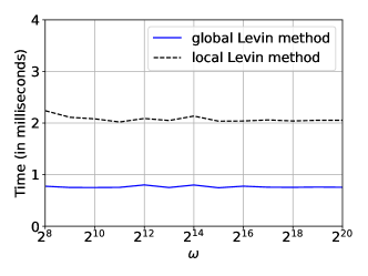
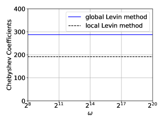
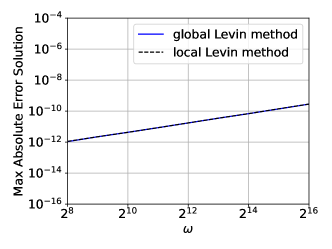
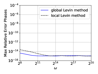
Figure 1: The results of the experiments of Subsection 5.1. The upper-left plot gives the time required by each of our methods as a function of the parameter $\omega$. The upper-right plot reports the number of Chebyshev coefficients required to represent the slowly-varying phase functions as a function of $\omega$. The lower-left plot reports the largest observed absolute error in the solutions of the initial value problem for (40) obtained using each of our methods. The plot on the lower right gives the largest observed relative error in the slowly-varying phase functions constructed by our algorithms. The plots in the upper-right and lower-left appear to have only one line because the solutions obtained by the local and global Levin methods closely coincide.

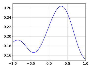
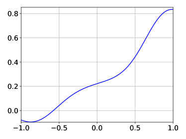
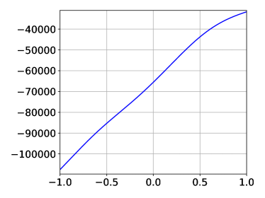
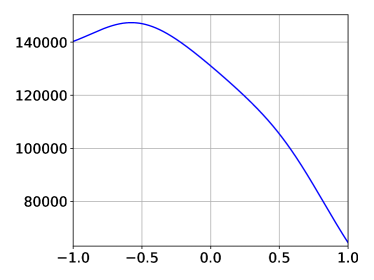
(a) The derivatives of the two slowly-varying phase functions produced by applying the global Levin method to Problem (40) of Subsection 5.1 when $\omega=2^{16}$. Each column corresponds to one of the phase functions, with the real part appearing in the first row and the imaginary part in the second.

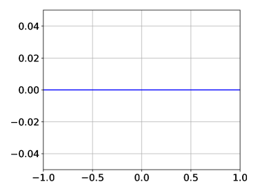
(b) The eigenvalues $\lambda_{1}(t),\lambda_{2}(t)$ of the coefficient matrix corresponding to Equation (40) of Subsection 5.1 when $\omega=2^{16}$. Each column corresponds to one of the eigenvalues, with the real part appearing in the first row and the imaginary part in the second.

Figure 2: Plots of some of the phase functions and eigenvalues which arose in the course of the experiments of Subsection 5.1.

5.2 An initial value problem for a third order equation

In this experiments, we considered the equation

$$y^{\prime\prime\prime}(t)+q_{2}(\omega,t)y^{\prime\prime}(t)+q_{1}(\omega,t)y^{\prime}(t)+q_{0}(\omega,t)y(t)=0,$$ (43)

where

$$q_{0}(\omega,t) =\frac{4\omega^{3}\left(i\omega\sin^{2}(t)+i\omega+\sin(t)\right)}{\left(t^{2}+1\right)\left(\omega e^{t}+1\right)},$$ (44)

$$q_{1}(\omega,t) =\frac{\omega\left(\omega\left(4\omega t^{2}+\omega e^{t}+1\right)+\left(\omega\left(4t^{2}+e^{t}+4\right)+1\right)\sin(t)(\omega\sin(t)-i)\right)}{\left(t^{2}+1\right)\left(\omega e^{t}+1\right)}\ \ \ \mbox{and}\ \ \$$

$$q_{2}(\omega,t) =i\omega\left(\frac{4\omega}{\omega e^{t}+1}+\frac{1}{t^{2}+1}-1\right)-i\omega\sin^{2}(t)-\sin(t).$$

At the point $0$, the eigenvalues of the coefficient matrix for (43) are given by the formulas

$$\lambda_{1}(0)=-\frac{4i\omega^{2}}{1+\omega},\ \ \ \lambda_{2}(0)=-i\omega\ \ \ \mbox{and}\ \ \ \lambda_{1}(0)=i\omega.$$ (45)

Plots of the eigenvalues $\lambda_{1}(t),\lambda_{2}(t),\lambda_{3}(t)$ of the coefficient matrix for (43) when $\omega=2^{16}$ can be found in Figure 4 .

In the first experiment, for each $\omega=2^{8},2^{9},\ldots,2^{16}$, we we used the local Levin method and the global Levin method to compute solutions of (43). We then measured the errors in each obtained solution at $10,000$ equispaced points in the interval $[-1,1]$ by comparison with a reference solution constructed via the standard solver described in Appendix A. In the second experiment, for each $\omega=2^{8},2^{9},\ldots,2^{20}$, we constructed slowly-varying phase functions for (43) over the interval $[-1,1]$ by running both the global and local Levin methods using double precision arithmetic. We then measured the relative errors in each obtained phase function at $10,000$ equispaced points in the interval $[-1,1]$ by comparison with phase functions constructed by applying the global Levin method to (43), but this time using extended precision arithmetic to perform the calculations. Figure 3 gives the results of these two experiments. Figure 5 contains plots of the derivatives of the slowly-varying phase functions produced by global Levin method when $\omega=2^{16}$.

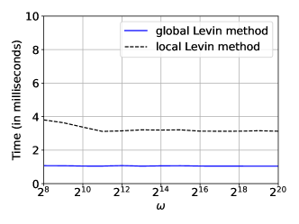
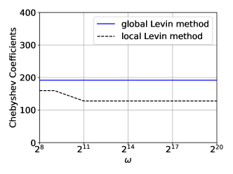
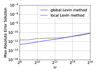
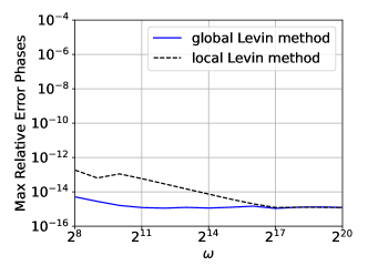
Figure 3: The results of the experiments of Subsection 5.2. The upper-left plot gives the time required by each of our methods as a function of the parameter $\omega$. The upper-right plot reports the number of Chebyshev coefficients required to represent the slowly-varying phase functions as a function of $\omega$. The lower-left plot reports the largest observed absolute error in the solution of the initial value problem for (43), again as a function of $\omega$. Finally, the plot on the lower right gives the largest observed relative error in the slowly-varying phase functions constructed by our algorithms.

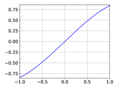
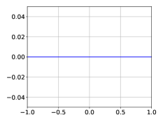
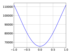
Figure 4: The eigenvalues $\lambda_{1}(t),\lambda_{2}(t),\lambda_{3}(t)$ of the coefficient matrix corresponding to Equation (43) of Subsection 5.2 when the parameter $\omega$ is equal to $2^{16}$. Each column corresponds to one of the eigenvalues, with the real part appearing in the first row and the imaginary part in the second.

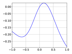
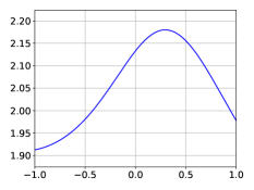
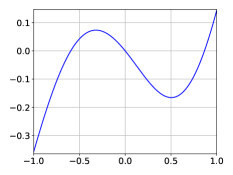
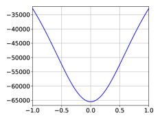
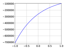
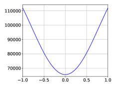
Figure 5: The derivatives of the three slowly-varying phase functions produced by applying the global Levin method to Equation (43) of Subsection 5.2 when the parameter $\omega$ is equal to $2^{16}$. Each column corresponds to one of the phase functions, with the real part appearing in the first row and the imaginary part in the second.

5.3 A boundary value problem for a third order equation

In the experiments described in this section, we considered the equation

$$y^{\prime\prime\prime}(t)-(1+2i\omega)(1+\sin^{2}(2t))\,y^{\prime\prime}(t)+(3i\omega+\omega^{2})\frac{1}{1-\frac{t}{2}}\,y^{\prime}(t)+(2\omega^{2}-2i\omega^{3})\frac{\exp(t)}{1+t^{4}}\,y(t)=0.$$ (46)

The eigenvalues of the coefficient matrix for (46) at the point $0$ are

$$\lambda_{1}(0)=i\omega,\ \ \ \lambda_{2}(0)=2i\omega\ \ \ \mbox{and}\ \ \ \lambda_{3}(0)=1-i\omega.$$ (47)

Plots of the eigenvalues $\lambda_{1}(t),\lambda_{2}(t),\lambda_{3}(t)$ of the coefficient matrix for (46) when $\omega=2^{16}$ can be found in Figure 8 .

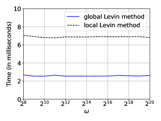
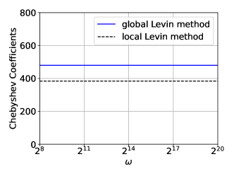
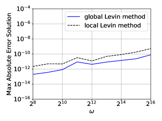
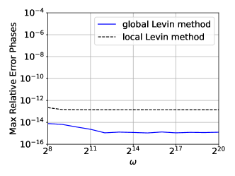
Figure 6: The results of the experiments of Subsection 5.3. The upper-left plot gives the time required by each of our methods as a function of the parameter $\omega$. The upper-right plot reports the number of Chebyshev coefficients required to represent the slowly-varying phase functions as a function of $\omega$. The lower-left plot reports the largest observed absolute error in the solution of a boundary value problem for (46), again as a function of $\omega$. Finally, the plot on the lower right gives the largest observed relative error in the slowly-varying phase functions constructed by our algorithms.

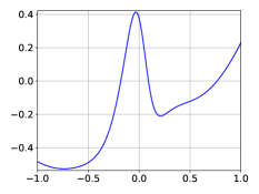
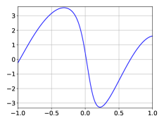
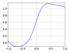
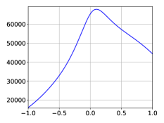
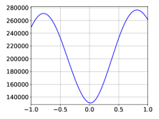
Figure 7: The derivatives of the three slowly-varying phase functions produced by applying the global Levin method to Equation (46) of Subsection 5.3 when the parameter $\omega$ is equal to $2^{16}$. Each column corresponds to one of the phase functions, with the real part appearing in the first row and the imaginary part in the second.

In the first experiment, for each $\omega=2^{8},2^{9},\ldots,2^{16}$, we we used the local Levin method and the global Levin method to compute solutions of (46) over the interval $[-1,1]$ subject to the conditions

$$y(-1)=y(1)=1\ \ \ \mbox{and}\ \ \ y^{\prime}(-1)=0.$$ (48)

We then measured the errors in each obtained solution at $10,000$ equispaced points in the interval $[-1,1]$ by comparison with a reference solution constructed via the standard solver described in Appendix A. In the second experiment, for each $\omega=2^{8},2^{9},\ldots,2^{20}$, we constructed slowly-varying phase functions for (46) over the interval $[-1,1]$ by running both the global and local Levin methods using double precision arithmetic (as usual). We then measured the relative errors in each obtained phase function at $10,000$ equispaced points in the interval $[-1,1]$ by comparison with phase functions constructed by applying the global Levin method to (46), but this time using extended precision arithmetic to perform the calculations. Figure 6 gives the results of these two experiments. Figure 7 contains plots of the derivatives of the slowly-varying phase functions produced by global Levin method when $\omega=2^{16}$.

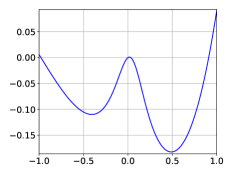
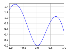
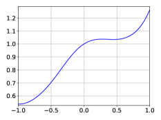
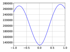
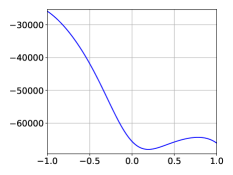
Figure 8: The eigenvalues $\lambda_{1}(t),\lambda_{2}(t),\lambda_{3}(t)$ of the coefficient matrix corresponding to Equation (46) of Subsection 5.3 when the parameter $\omega$ is equal to $2^{16}$. Each column corresponds to one of the eigenvalues, with the real part appearing in the first row and the imaginary part in the second.

5.4 An initial value problem for a fourth order equation

In the experiments described in this section, we considered the equation

$$y^{\prime\prime\prime\prime}(t)+\left(-5i\omega(1+t^{2})+5\omega^{2}\,\frac{8+\cos^{4}(3t)}{2+t^{4}}\right)y^{\prime\prime}(t)+4\omega^{4}\,\frac{2+\sin(3t)}{2+t}y(t)=0.$$ (49)

We have the following formulas for the eigenvalues of the coefficient matrix at the point $0$:

$$\lambda_{1}(0) =\sqrt{\frac{5i\omega-5\omega^{2}+\omega\sqrt{-25-50i\omega+9\omega^{2}}}{2}}\sim-i\omega+\frac{5}{6}+\mathcal{O}\left(\frac{1}{\omega}\right)$$

$$\lambda_{2}(0) =-\sqrt{\frac{5i\omega-5\omega^{2}+\omega\sqrt{-25-50i\omega+9\omega^{2}}}{2}}\sim i\omega-\frac{5}{6}+\mathcal{O}\left(\frac{1}{\omega}\right)$$

$$\lambda_{3}(0) =\sqrt{\frac{5i\omega-5\omega^{2}-\omega\sqrt{-25-50i\omega+9\omega^{2}}}{2}}\sim 2i\omega+\frac{5}{3}+\mathcal{O}\left(\frac{1}{\omega}\right)$$

$$\lambda_{4}(0) =-\sqrt{\frac{5i\omega-5\omega^{2}-\omega\sqrt{-25-50i\omega+9\omega^{2}}}{2}}\sim-2i\omega-\frac{5}{3}+\mathcal{O}\left(\frac{1}{\omega}\right).$$

In the first experiment, for $\omega=2^{8},2^{9},\ldots,2^{16}$, we used both the global Levin method and the local Levin method to solve (49) over the interval $[-1,1]$ subject to the conditions

$$y(0)=1,\ \ \ y^{\prime}(0)=i\omega,\ \ \ y^{\prime\prime}(0)=-\omega^{2}\ \ \ \mbox{and}\ \ \ y^{\prime\prime\prime}(0)=-i\omega^{3}.$$ (50)

Then we measured the errors in each obtained solution at $10,000$ equispaced points in the interval $[-1,1]$ by comparison with reference solutions constructed via the standard solver described in Appendix A. In the second experiment, for each $\omega=2^{8},2^{9},\ldots,2^{20}$, we constructed slowly-varying phase functions for (49) over the interval $[-1,1]$ by running both the global and local Levin methods using double precision arithmetic (as usual). We then measured the relative errors in each obtained phase function at $10,000$ equispaced points in the interval $[-1,1]$ by comparison with phase functions constructed by applying the global Levin method to (49), but this time using extended precision arithmetic to perform the calculations. Figure 9 gives the results of these two experiments. Figure 10 contains plots of the derivatives of the slowly-varying phase functions produced by global Levin method when $\omega=2^{16}$.

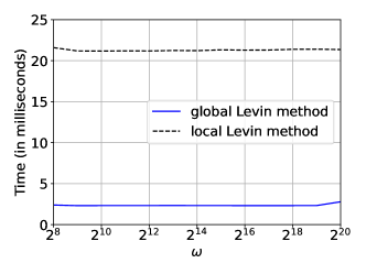
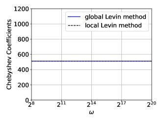
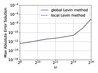
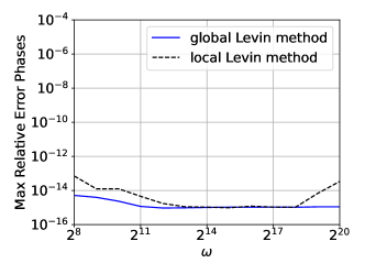
Figure 9: The results of the experiment of Subsection 5.4. The upper-left plot gives the time required by each of our methods as a function of the parameter $\omega$. The upper-right plot reports the number of Chebyshev coefficients required to represent the slowly-varying phase functions as a function of $\omega$. The lower-left plot reports the largest observed absolute error in the solution of the initial value problem for (49), again as a function of $\omega$. The plot on the lower right gives the largest observed relative error in the slowly-varying phase functions constructed by our algorithms. The plot on the lower left appears to have only one line because the solutions generated by the local and global Levin methods closely coincide.

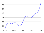
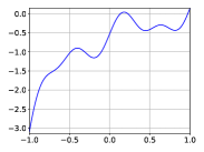
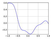
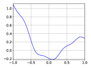
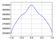
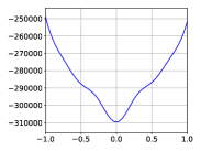
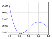
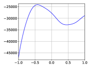
Figure 10: The derivatives of the four slowly-varying phase functions produced by applying the global Levin method to Equation (49) of Subsection 5.4 when the parameter $\omega$ is equal to $2^{16}$. Each column corresponds to one of the phase functions, with the real part appearing in the first row and the imaginary part in the second.

5.5 An equation whose coefficient matrix has eigenvalues with large real parts

The experiment of this section concerns the fourth order differential equation

$$y^{\prime\prime\prime\prime}(t)+\omega^{4}\left(\frac{2+\cos(7t)^{2}}{1+t^{4}}\right)y(t)=0.$$ (51)

When $\omega$ is large, some of the eigenvalues of the corresponding coefficient matrix have real parts of large magnitude, with the consequence that almost all initial and boundary value problems for (51) are highly ill-conditioned. This makes testing the accuracy of the obtained phase functions by using them to construct solutions of (51) and comparing the results to reference solutions virtually impossible. Instead, we assess the accuracy of the phase functions using our second approach, via comparison with phase functions constructed by our algorithms using extended precision arithmetic.

More explicitly, for each $\omega=2^{8},2^{9},\ldots,2^{20}$, we constructed slowly-varying phase functions for (51) over the interval $[-1,1]$ by running the global method using double precision arithmetic. We then measured the relative errors in each obtained phase function at $10,000$ equispaced points in the interval $[-1,1]$ by comparison with phase functions constructed by applying the global Levin method to (51), but this time using extended precision arithmetic to perform the calculations. Figure 11 gives the results of these experiments. Plots of the eigenvalues $\lambda_{1}(t),\lambda_{2}(t),\lambda_{3}(t),\lambda_{4}(t)$ of the coefficient matrix for (51) when $\omega=2^{16}$ can be found in Figure 12 .

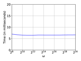
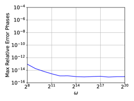
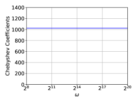
Figure 11: The results of the experiment of Subsection 5.5. The leftmost plot gives the time required by the global Levin method as a function of the parameter $\omega$. The middle plot reports the maximum relative error in the slowly-varying phase functions. The plot on the right shows the number of Chebyshev coefficients required to represent the slowly-varying phase functions, again as a function of $\omega$.

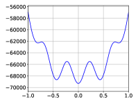
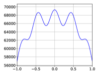
Figure 12: The eigenvalues $\lambda_{1}(t),\lambda_{2}(t),\lambda_{3}(t),\lambda_{4}(t)$ of the coefficient matrix for (51) when the parameter $\omega$ is equal to $2^{16}$. Each column corresponds to one of the eigenvalues, with the real part appearing in the first row and the imaginary part in the second.

5.6 An equation whose coefficient matrix has eigenvalues of small magnitude

In the experiment described in this section, we solved the equation

$$y^{\prime\prime\prime}(t)-i\omega\left(1+t^{2}\right)y^{\prime\prime}(t)+\frac{2+t}{1+t^{2}}\,y^{\prime}(t)+i\omega\log\left(\frac{3}{2}+t\right)y(t)=0$$ (52)

over the interval $[-1,1]$ subject to the conditions

$$y(0)=1,\ \ \ y^{\prime}(0)=-i\omega,\ \ \ y^{\prime\prime}(0)=-\omega^{2}.$$ (53)

The coefficient matrix corresponding to (52) has eigenvalues of small magnitude, and, as discussed in the introduction, the global Levin method encounters difficulties in such cases. In particular, the obtained functions can be discontinuous across the boundaries of the subintervals set by the adaptive discretization scheme. This is readily apparent in Figure 14, which contains plots of the functions that result when the global Levin method is applied to (52) with $\omega=2^{16}$. Fortunately, the local Levin method has no difficulties in this case; Figure 15 contains plots of the functions obtained when it is applied to (52) with $\omega=2^{16}$.

For each $\omega=2^{8},2^{9},\ldots,2^{20}$, we used the local Levin method to solve (52) subject to (53). The error in each obtained solution was measured at $10,000$ equispaced points on the interval $[-1,1]$. Figure 13 gives the results. Plots of the eigenvalues $\lambda_{1}(t),\lambda_{2}(t),\lambda_{3}(t),\lambda_{4}(t)$ of the coefficient matrix for (52) when $\omega=2^{16}$ can be found in Figure 15 .

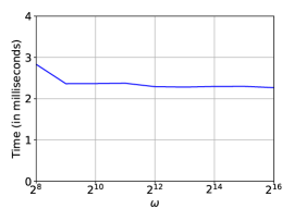
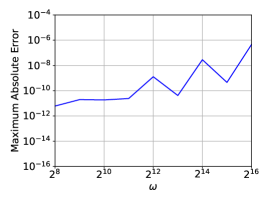
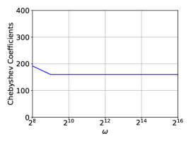
Figure 13: The results of the experiment of Subsection 5.6. The leftmost plot gives the time required by the local Levin method as a function of the parameter $\omega$. The plot in the middle reports the largest observed absolute error in the solution of the initial value problem for (52) as a function of $\omega$. The rightmost plot shows the total number of Chebyshev coefficients required to represent the slowly-varying phase functions, again as a function of $\omega$.

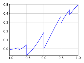
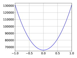
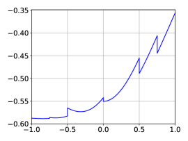
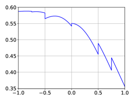
Figure 14: The degenerate results obtained when the global Levin method is applied to Equation (52) of Subsection 5.6 with $\omega=2^{16}$. In this case, the coefficient matrix admits eigenvalues of small magnitude and the functions obtained by the global Levin method are contaminated by elements of the nullspaces of the linearized operators which arise in the course of the Newton procedure. Each column corresponds to one of the phase functions, with the real part appearing in the first row and the imaginary part in the second.

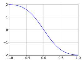
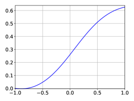
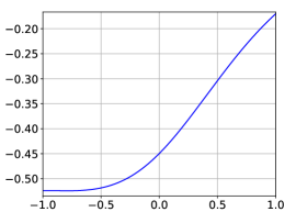
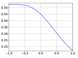
Figure 15: The derivatives of the slowly-varying phase functions obtained when the local Levin method is applied to Equation (52) of Subsection 5.6 with $\omega=2^{16}$. Even though the coefficient matrix admits eigenvalues of small magnitude, the local Levin method is still able to construct the desired slowly-varying phase functions. Each column corresponds to one of the phase functions, with the real part appearing in the first row and the imaginary part in the second.

5.7 A system of two differential equations in two unknowns

It is well known that essentially any system of $n$ linear ordinary differential equations in $n$ unknowns can be transformed into an $n^{th}$ order linear scalar differential equation (see, for instance, Kolchin ). As a consequence, the algorithms of this paper can be used to solve many such systems in time independent of the magnitudes of the eigenvalues of their coefficient matrices. In the experiment of this section, we solved the system of differential equations

$$\mathbf{y}^{\prime}(t)=\left(\begin{array}[]{cc}1+t^{2}&\frac{1}{1+t^{4}}\\ \frac{-\omega}{1+t^{2}}&\frac{-i\omega(2+t)}{5+t}\end{array}\right)\mathbf{y}(t)$$ (54)

on the interval $[-1,1]$ subject to the condition

$$\mathbf{y}(0)=\left(\begin{array}[]{c}1\\ 1\end{array}\right).$$ (55)

We found that letting

$$\mathbf{w}(t)=\Phi(t)\mathbf{y}(t)$$ (56)

with

$$\Phi(t)=\left(\begin{array}[]{cc}0&1\\ \frac{-\omega}{1+t^{2}}&\frac{-i\omega(2+t)}{5+t}\end{array}\right)$$ (57)

transforms (54) into the system

$$\mathbf{w}^{\prime}(t)=\left(\begin{array}[]{cc}0&1\\ -q_{0}(t)&-q_{1}(t)\end{array}\right)\mathbf{w}(t),$$ (58)

where

$$q_{0}(t)=\frac{1}{(t+5)^{2}\left(t^{2}+1\right)\left(t^{4}+1\right)}\left(-i\omega t^{10}-7i\omega t^{9}-12i\omega t^{8}-12i\omega t^{7}-5i\omega t^{6}+\right.$$

$$\left.6i\omega t^{5}-19i\omega t^{4}-12i\omega t^{3}+(1-4i)\omega t^{2}+(10+13i)\omega t+(25-7i)\omega\right)$$

and

$$q_{1}(t)=\frac{i\omega(t+2)}{t+5}-t^{2}+\frac{2t}{t^{2}+1}-1.$$

Of course, (58) is equivalent to the scalar equation

$$z^{\prime\prime}(t)+q_{1}(t)z^{\prime}(t)+q_{0}(t)z(t)=0$$ (59)

with $z$ related to $\mathbf{w}=\left(\begin{array}[]{cc}w_{1}(t)&w_{2}(t)\end{array}\right)$ via the formulas

$$z(t)=w_{1}(t)\ \ \ \mbox{and}\ \ \ z^{\prime}(t)=w_{2}(t).$$ (60)

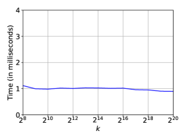
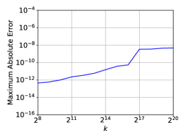
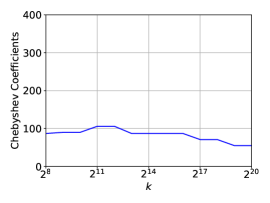
Figure 16: The results of the experiment of Subsection 5.7. The leftmost plot gives the time required by each of our methods as a function of the parameter $\omega$. The plot in the middle reports the largest observed error in the solution as a function of $\omega$. The plot on the right shows the total number of Chebyshev coefficients required to represent the slowly-varying phase functions, again as a function of $\omega$.

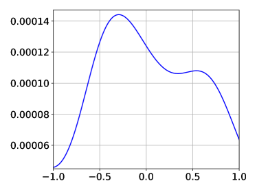
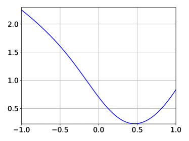
(a) The derivatives of the two slowly-varying phase functions produced by applying the global Levin method to the scalar equation (59) obtained from the system (54) when $\omega=2^{16}$. Each column corresponds to one of the phase functions, with the real part appearing in the first row and the imaginary part in the second.

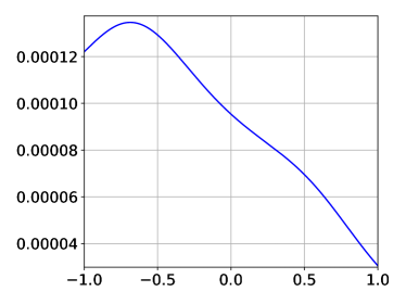
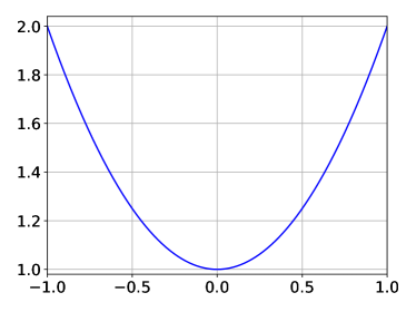
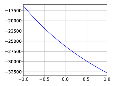
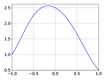
(b) The eigenvalues $\lambda_{1}(t),\lambda_{2}(t)$ of the coefficient matrix of the system (54) when $\omega=2^{16}$. Each column corresponds to one of the eigenvalues, with the real part appearing in the first row and the imaginary part in the second.

Figure 17: Plots of some of the phase functions and eigenvalues which arose in the course of the experiments of Subsection 5.7.

For each $\omega=2^{8},2^{9},\ldots,2^{20}$, we followed the following procedure. First, we used the local Levin method to construct slowly-varying phase functions $\psi_{1},\psi_{2}$ such that

$$z_{1}(t)=\exp(\psi_{1}(t))\ \ \ \mbox{and}\ \ z_{2}(t)=\exp(\psi_{2}(t))$$ (61)

form a basis in the space of solutions of (59) over the interval $[-1,1]$. Next, we let formed the two corresponding solutions

$$\mathbf{y}_{1}(t)=\Phi^{-1}(t)\left(\begin{array}[]{c}z_{1}(t)\\ z_{1}^{\prime}(t)\end{array}\right)\ \ \ \mbox{and}\ \ \ \mathbf{y}_{2}(t)=\Phi^{-1}(t)\left(\begin{array}[]{c}z_{2}(t)\\ z_{2}^{\prime}(t)\end{array}\right)$$ (62)

of (54) and found constants $c_{1}$ and $c_{2}$ such that

$$c_{1}\mathbf{y}_{1}(0)+c_{2}\mathbf{y}_{2}(0)=\left(\begin{array}[]{c}1\\ 1\end{array}\right)$$ (63)

by solving the obvious system of linear algebraic equations. Finally, we constructed a reference solution for the problem using the standard solver of Appendix A and compared its value with that of $c_{1}\mathbf{y}_{1}(t)+c_{2}\mathbf{y}_{2}(t)$ at $10,000$ equispaced points on the interval $[-1,1]$. Figure 16 gives the results. Figure 17(a) contains plots of the slowly-varying phase functions for (59) which were constructed when $\omega=2^{16}$. Figure 17(b) contains plots of the eigenvalues of the matrix (54) when $\omega=2^{16}$.

6 Conclusions

We have introduced two related approaches for solving initial and boundary value problems for a large class of scalar ordinary differential equations. They are both based on the principle which underpins the classical Levin method for calculating oscillatory integrals, namely, that inhomogeneous linear ordinary differential equations with slowly-varying coefficients and a slowly-varying right-hand side admit slowly-varying solutions regardless of the magnitudes of the coefficients. Using Newton’s method, we were able to apply this principle to the nonlinear Riccati equation in order to rapidly compute slowly-varying phase functions for scalar ordinary differential equations.

Both of our methods for computing phase functions achieve high-accuracy and high order convergence, and run in time independent of the magnitude of the equation’s coefficients. One of the approaches, the global Levin method, fails when the coefficient matrix has eigenvalues of small magnitude. The other approach, the local Levin method, is slightly less accurate and slightly slower than the global method in most cases in which both apply, but it does not suffer from this defect.

As is clear from our plots, the solutions of the Riccati equation possess various symmetries. We have made no attempt to exploit them to accelerate our algorithm, or to make a number of other obvious speed improvements. Indeed, our implementations are reference codes are meant to demonstrate the basic properties of our algorithms and are not designed to achieve the greatest possible speed.

We encountered difficulties in testing the accuracy of our algorithms. For the most part, we did so by using the obtained phase functions to solve an initial or boundary value problem for a differential equation and comparing the result to that obtained by a standard solver. This approach has serious limitations, however, due to the poor performance exhibited by standard methods when applied to most of the problems discussed here. The problems were so severe, in fact, that we resorted to also measuring the accuracy of our phase functions by comparison with results obtained by running our algorithms using extended precision arithmetic.

There are many obvious applications of this work to evaluation of special functions, calculation of special function transforms and the solution of physical problems which should be explored. Moreover, because essentially any system of $n$ ordinary differential equations in $n$ unknowns can be transformed into an $n^{th}$ order scalar equation, it should be possible to use the algorithm of this paper to solve a large class of systems of differential equations in time time independent of the magnitudes of the eigenvalues of their coefficient matrices. We have given one such example in this paper, but further development of this approach is required in order to obtain a solver which can be applied to a large class of equations.

7 Acknowledgments

JB was supported in part by NSERC Discovery grant RGPIN-2021-02613.

8 Data availability statement

The datasets generated during and/or analysed during the current study are available from the corresponding author on reasonable request.

Appendix A An adaptive spectral solver for ordinary differential equations

In this appendix, we detail a standard adaptive spectral method for solving ordinary differential equations. It is used by the local Levin method, and to calculate reference solutions in our numerical experiments. We describe its operation in the case of the initial value problem

$$\left\{\begin{aligned} \bm{y}^{\prime}(t)&=F(t,\bm{y}(t)),\ \ \ a<t<b,\\ \bm{y}(a)&=\bm{v}\end{aligned}\right.$$ (64)

where $F:\mathbb{R}^{n+1}\to\mathbb{C}^{n}$ is smooth and $\bm{v}\in\mathbb{C}^{n}$. However, the solver can be easily modified to produce a solution with a specified value at any point $\eta$ in $[a,b]$.

The solver takes as input a positive integer $k$, a tolerance parameter $\epsilon$, an interval $(a,b)$, the vector $\bm{v}$ and a subroutine for evaluating the function $F$. It outputs $n$ piecewise $(k-1)^{st}$ order Chebyshev expansions, one for each of the components $y_{i}(t)$ of the solution $\bm{y}$ of (64).

The solver maintains two lists of subintervals of $(a,b)$: one consisting of what we term “accepted subintervals” and the other of subintervals which have yet to be processed. A subinterval is accepted if the solution is deemed to be adequately represented by a $(k-1)^{st}$ order Chebyhev expansion on that subinterval. Initially, the list of accepted subintervals is empty and the list of subintervals to process contains the single interval $(a,b)$. It then operates as follows until the list of subintervals to process is empty:

1. Find, in the list of subinterval to process, the interval $(c,d)$ such that $c$ is as small as possible and remove this subinterval from the list.

2. Solve the initial value problem

   $$\left\{\begin{aligned} \bm{u}^{\prime}(t)&=F(t,\bm{u}(t)),\ \ \ c<t<d,\\ \bm{u}(c)&=\bm{w}\end{aligned}\right.$$ (65)

   If $(c,d)=(a,b)$, then we take $\bm{w}=\bm{v}$. Otherwise, the value of the solution at the point $c$ has already been approximated, and we use that estimate for $\bm{w}$ in (65).

   If the problem is linear, a straightforward Chebyshev integral equation method (see, for instance, GreengardSolver ) is used to solve (65). Otherwise, the trapezoidal method is first used to produce an initial approximation $\bm{y_{0}}$ of the solution and then Newton’s method is applied to refine it. The linearized problems are solved using a Chebyshev integral equation method.

   In any event, the result is a set of $(k-1)^{st}$ order Chebyshev expansions

   $$u_{i}(t)\approx\sum_{j=0}^{k-1}\lambda_{ij}\ T_{j}\left(\frac{2}{d-c}t+\frac{c+d}{c-d}\right),\ \ \ i=1,\ldots,n,$$ (66)

   approximating the components $u_{1},\ldots,u_{n}$ of the solution of (65).

3. Compute the quantities

   $$\frac{\sqrt{\sum_{j=\lfloor k/2\rfloor+1}^{k-1}\left|\lambda_{ij}\right|^{2}}}{\sqrt{\sum_{j=0}^{k-1}\left|\lambda_{ij}\right|^{2}}},\ \ \ i=1,\ldots,n,$$ (67)

   where the $\lambda_{ij}$ are the coefficients in the expansions (66). If any of the resulting values is larger than $\epsilon$, then we split the subinterval into two halves $\left(c,\frac{c+d}{2}\right)$ and $\left(\frac{c+d}{2},d\right)$ and place them on the list of subintervals to process. Otherwise, we place the subinterval $(c,d)$ on the list of accepted subintervals.

At the conclusion of this procedure, we have $(k-1)^{st}$ order piecewise Chebyshev expansions for each component of the solution, with the list of accepted subintervals determining the partition for each expansion.

References

- (1) Aurentz, J., Mach, T., Robol, L., Vanderbril, R., and Watkins, D. S. Fast and backward stable computation of roots of polynomials, part II: Backward error analysis; companion matrix and companion pencil. SIAM Journal on Matrix Analysis and Applications 39 (2018), 1245–1269.
- (2) Aurentz, J., Mach, T., Vanderbril, R., and Watkins, D. S. Fast and backward stable computation of roots of polynomials. SIAM Journal on Matrix Analysis and Applications 36 (2015), 942–973.
- (3) Bremer, J. On the numerical solution of second order differential equations in the high-frequency regime. Applied and Computational Harmonic Analysis 44 (2018), 312–349.
- (4) Bremer, J. Phase function methods for second order linear ordinary differential equations with turning points. Applied and Computational Harmonic Analysis 65 (2023), 137–169.
- (5) Chen, S., Serkh, K., and Bremer, J. The adaptive Levin method. arXiv 2209.14561 (2022).
- (6) Greengard, L. Spectral integration and two-point boundary value problems. SIAM Journal of Numerical Analysis 28 (1991), 1071–1080.
- (7) Iserles, A. On the global error of discretization methods for highly-oscillatory ordinary differential equations. BIT 32 (2002), 561–599.
- (8) Iserles, A., and Nørsett, S. P. On the solution of linear differential equations in Lie groups. Philosophical Transactions: Mathematical, Physical and Engineering Sciences 357, 1754 (1999), 983–1019.
- (9) Kolchin, E. Differential Algebraic Groups. Academic Press, Orlando, Florida, 1985.
- (10) Levin, D. Procedures for computing one- and two-dimensional integrals of functions with rapid irregular oscillations. Mathematics of Computation 38 (1982), 531–5538.
- (11) Li, J., Wang, X., and Wang, T. A universal solution to one-dimensional oscillatory integrals. Science in China Series F: Information Sciences 51 (2008), 1614–1622.
- (12) Li, J., Wang, X., Wang, T., and Xiao, S. An improved Levin quadrature method for highly oscillatory integrals. Applied Numerical Mathematics 60, 8 (2010), 833–842.
- (13) Magnus, W. On the exponential solution of differential equations for a linear operator. Communications on Pure and Applied Mathematics 7 (1954), 649–673.
- (14) Miller, P. D. Applied Asymptotic Analysis. American Mathematical Society, Providence, Rhode Island, 2006.
- (15) Spigler, R. Asymptotic-numerical approximations for highly oscillatory second-order differential equations by the phase function method. Journal of Mathematical Analysis and Applications 463 (2018), 318–344.
- (16) Spigler, R., and Vianello, M. A numerical method for evaluating the zeros of solutions of second-order linear differential equations. Mathematics of Computation 55 (1990), 591–612.
- (17) Spigler, R., and Vianello, M. The phase function method to solve second-order asymptotically polynomial differential equations. Numerische Mathematik 121 (2012), 565–586.
- (18) Wasow, W. Asymptotic expansions for ordinary differential equations. Dover, 1965.