Exploring Non–commutativity as a Perturbation in the Schwarzschild Black Hole: Quasinormal Modes, Scattering, and Shadows

Abstract

In this work, by a novel approach to studying the scattering of a Schwarzschild black hole, the non–commutativity is introduced as a perturbation. We begin by reformulating the Klein–Gordon equation for the scalar field in a new form that takes into account the deformed non–commutative spacetime. Using this formulation, an effective potential for the scattering process is derived. To calculate the quasinormal modes, we employ the WKB method and also utilize fitting techniques to investigate the impact of non–commutativity on the scalar quasinormal modes. We thoroughly analyze the results obtained from these different methods. Moreover, the greybody factor and absorption cross section are investigated. Additionally, we explore the behavior of null geodesics in the presence of non–commutativity. Specifically, we examine the photonic, and shadow radius as well as the light trajectories for different non–commutative parameters. Therefore, by addressing these various aspects, we aim to provide a comprehensive understanding of the influence of non–commutativity on the scattering of a Schwarzschild–like black hole and its implications for the behavior of scalar fields and light trajectories.

Keywords: Non–commutativity; Black hole; Quasinormal Mode; WKB methods; Greybody factor; Absorption cross section; Shadow radius; Geodesics.

1 Introduction

Non–commutative spacetime has been a subject of interest for researchers in gravity theories [1, 2, 3, 4]. One significant application of such geometry is certainly in the context of black holes.This spacetime is described by the relation $\left[x^{\mu},x^{\nu}\right]=i\Theta^{\mu\nu}$, where $x^{\mu}$ represents the operators for spacetime coordinates and $\Theta^{\mu\nu}$ denotes an anti–symmetric constant tensor. Several methods have been developed to incorporate non–commutativity into gravity theories [5, 6, 7, 8, 9, 10, 11, 12, 13, 14]. In the literature, there exists a formalism which involves the use of the non–commutative gauge de Sitter (dS) group, SO(4,1), in conjunction with the Poincarè group, ISO(3,1), regarding the Seiberg–Witten (SW) map approach[15, 16, 17]. With it, Chaichian et al. [18] derived a deformed metric for the Schwarzschild black hole. On the other hand, Nicolini et al.[9] found that the non–commutative effects can be considered solely as consequence of the matter source term without altering the Einstein tensor part of the field equation. Consequently, they can be implemented by replacing the mass density of the point–like function on the right side of the Einstein equation with a Gaussian smeared matter distribution [9]. This aspect takes the form ${\rho_{\Theta}}=M{(4\pi\Theta)^{-\frac{3}{2}}}e^{-\frac{{{r^{2}}}}{{4\Theta}}}$, or alternatively, a Lorentzian distribution[19] with ${\rho_{\Theta}}=M\sqrt[\ ]{\Theta}{\pi^{-\frac{3}{2}}}{({r^{2}}+\pi\Theta)^{-2}}$, where $M$ is the total mass distribution [20, 21, 22, 23, 24]. In Ref. [25] the authors introduced a general method for finding scalar QNMs of non–separable black hole spacetime which is close to the Kerr background. Recently, Ref. [26] introduced a deformed mass derived from the deformed metric proposed by Chaichian et al. [18].
The study of gravitational waves and their spectra over the last years has attracted lots of attentions [27, 28, 29, 30, 31, 32, 33], particularly, with the advancements in gravitational wave detectors such as VIRGO and LIGO. These ones have provided valuable insights into black hole physics [34, 35, 36, 37, 38]. One aspect of this research involves investigating the quasinormal modes (QNMs), which are complex oscillation frequencies that arise in the response of black holes to initial perturbations. These frequencies can be obtained under specific boundary conditions [39, 40]. Various studies have explored the scattering and QNMs in non–commutative spacetime by considering deformed mass density instead of deformed spacetime with a non–commutative (NC) parameter [41, 42, 2, 43, 44, 45]. However, the calculation of quasinormal modes based on a deformed metric has not been extensively addressed in the literature. In this research, our aim is to investigate the scattering process of a Schwarzschild black hole in a non–commutative spacetime [18]. To achieve this, we employ the WKB method [46, 47, 48, 49, 50, 51] to determine the quasinormal frequencies of massless scalar perturbations. Additionally, we calculate the greybody factor for the scalar field and examine the impact of non–commutativity on the absorption cross section.

Furthermore, exploring the geodesics and shadow radius to enhance our understanding of the gravitational lensing has gained attentions [52, 53, 54]. We explore these aspects of the Schwarzschild–like black hole in the non–commutative spacetime [3, 55, 56, 57, 58].

The structure of this paper is as follows: In Section 2, first we provide an overview of implementing non–commutative spacetime through the metric of the Schwarzschild–like black hole. After that, we focus on the massless Klein–Gordon equation, where we derive a Schrödinger–like form for the wave equation and find an effective potential. Section 3 is dedicated to obtaining the quasinormal modes of the non–commutative deformed Schwarzschild black hole using the WKB method, Pösch–Teller and Rosen–Morse fitting method. In Section 4, we calculate the greybody factor and absorption cross section concerning non–commutativity parameter. Section 5 addresses the null geodesic and shadow radius in non–commutative spacetime. Finally, we present the conclusions in Section 6.

2 Effective potential of deformed metric by non-commutativity

In this section, we discuss the non–commutative Schwarzschild black hole spacetime with correction terms. The metric, which takes into account all these features is given by $g_{ij}^{NC}=g_{ij}+\Theta^{2}h_{ij}^{NC}$, where $g_{ij}$ represent the original Schwarzschild black hole metric parameters and $h_{ij}^{NC}$s are the coefficients for the non–commutative correction term, as mentioned in Ref. [18, 16, 15]. Additionally, Ref. [59] introduces a remarkable proposal for a deformed Schwarzschild black hole metric that is both stationary and axisymmetric. The deformed metric, which incorporates a small dimensionless parameter $\epsilon$, can be expressed in the following form

$${{\hat{g}_{00}}} =-(1-\frac{{2M}}{r})(1+\epsilon{A_{j}}{{\mathop{\rm cos}\nolimits}^{j}}\theta),$$ (2.1)

$${{\hat{g}}_{11}} ={(1-\frac{{2M}}{r})^{-1}}(1+\epsilon{B_{j}}{{\mathop{\rm cos}\nolimits}^{j}}\theta),$$ (2.2)

$${{\hat{g}}_{22}} ={r^{2}}(1+\epsilon{C_{j}}{{\mathop{\rm cos}\nolimits}^{j}}\theta),$$ (2.3)

$${{\hat{g}}_{33}} ={r^{2}}{{\mathop{\rm sin}\nolimits}^{2}}\theta(1+\epsilon{D_{j}}{{\mathop{\rm cos}\nolimits}^{j}}\theta),$$ (2.4)

$${{\hat{g}}_{01}} =\epsilon{a_{j}}(r){{\mathop{\rm cos}\nolimits}^{j}}\theta,\quad{{\hat{g}}_{12}}=\epsilon{c_{j}}(r){{\mathop{\rm cos}\nolimits}^{j}}\theta,\quad\ {{\hat{g}}_{23}}=\epsilon{e_{j}}(r){{\mathop{\rm cos}\nolimits}^{j}}\theta,$$ (2.5)

$${{\hat{g}}_{02}} =\epsilon{b_{j}}(r){{\mathop{\rm cos}\nolimits}^{j}}\theta,\quad{{\hat{g}}_{13}}=\epsilon{d_{j}}(r){{\mathop{\rm cos}\nolimits}^{j}}\theta.$$ (2.6)

Influenced by the findings presented in Ref. [60], a novel methodology for handling NC spacetime is employed. We approach the NC Schwarzschild metric as a specific instance of the deformed Schwarzschild metric, denoted as $\hat{g}_{ij}={g_{ij}^{NC}}$. Furthermore, we assume that the small deformed parameter is equivalent to the NC parameter $(\epsilon=\Theta^{2})$. Consequently, the deformed coefficients of the metric are derived as indicated in Ref. [59, 60]

$${A_{0}}=\frac{{\alpha\left({8r-11\alpha}\right)}}{{16{r^{3}}\left({r-\alpha}\right)}},$$ (2.8)

$${B_{0}}=-\frac{{\alpha\left({4r-3\alpha}\right)}}{{16{r^{3}}\left({r-\alpha}\right)}},$$ (2.9)

$${C_{0}}=\frac{{2{r^{2}}-17\alpha\left({r-\alpha}\right)}}{{32{r^{3}}\left({r-\alpha}\right)}},$$ (2.10)

$${D_{0}}=-\frac{{\alpha\left({2r-\alpha}\right)}}{{16{r^{3}}\left({r-\alpha}\right)}},$$ (2.11)

$${A_{j}}={B_{j}}={C_{j}}=0\quad\text{and}\quad{D_{j}}=\frac{{1+{{\left({-1}\right)}^{j}}}}{{32{r^{2}}}}\quad\text{for}\quad j>0,$$ (2.12)

$${a_{j}}(r)={b_{j}}(r)={c_{j}}(r)={d_{j}}(r)=0.$$ (2.13)

Here, $\alpha$ is a constatnt given by $\alpha=2M$. Building upon this new approach, the upcoming section focuses on examining the evolution of the massless scalar perturbation field within NC metric, considering the deformed spacetime of the Schwarzschild black hole. To do so, we express the Klein–Gordon equation in the context of a curved spacetime as follows

$$\Box\psi=\frac{1}{{\sqrt[\ ]{-g}}}{\partial_{\mu}}(\sqrt[\ ]{-g}{g^{\mu\nu}}{\partial_{\nu}}\psi)=0.$$ (2.14)

Assuming two Killing vector $\partial_{t}$ and $\partial_{\phi}$ the wave function can be decomposed as

$$\psi=\int_{-\infty}^{\infty}{d\omega\sum\limits_{m=-\infty}^{\infty}{{e^{im\varphi}}D_{m,\omega}^{2}{\psi_{m,\omega}}(r,\theta){e^{-i\omega t}}}},$$ (2.15)

where $D_{m,\omega}^{2}{\psi_{m,\omega}}(r,\theta)=0$, $m$ and $\omega$ are the azimuthal number and the mode frequency, respectively. Now, if we decompose the operator $D_{m,\omega}^{2}{\psi_{m,\omega}}$ up to the first order of $\Theta^{2}$ [59, 60], we obtain

$$D_{m,\omega}^{2}=D_{(0)m,\omega}^{2}+{\Theta^{2}}D_{(1)m,\omega}^{2}.$$ (2.16)

Applying the metric coefficients from Eq. (2.8)- (2.13) in Eq. (2.14)

$$D_{(0)m,\omega}^{2} =-({\omega^{2}}-\frac{{{m^{2}}f}}{{{r^{2}}{{{\mathop{\rm sin}\nolimits}}^{2}}\theta}})-\frac{f}{{{r^{2}}}}{\partial_{r}}({r^{2}}f{\partial_{r}})-{{\mathop{\rm cos}\nolimits}^{j}}\theta({\partial_{r}}({r^{2}}f{\partial_{r}}))$$ (2.17)

$$-\frac{f}{{{r^{2}}{{{\mathop{\rm sin}\nolimits}}^{2}}\theta}}{\partial_{\theta}}({\mathop{\rm sin}\nolimits}\theta{\partial_{\theta}}),$$ (2.18)

$$D_{(1)m,\omega}^{2} =\frac{{{m^{2}}f}}{{{r^{2}}{{{\mathop{\rm sin}\nolimits}}^{2}}\theta}}({A_{j}}-{D_{j}}){{\mathop{\rm cos}\nolimits}^{j}}\theta-\frac{f}{{{r^{2}}}}({A_{j}}-{B_{j}}){{\mathop{\rm cos}\nolimits}^{j}}\theta({\partial_{r}}({r^{2}}f{\partial_{r}}))$$

$$-\frac{{{f^{2}}}}{{{r^{2}}}}({{A^{\prime}}_{j}}-{{B^{\prime}}_{j}}+{{C^{\prime}}_{j}}+{{D^{\prime}}_{j}}){{\mathop{\rm cos}\nolimits}^{j}}\theta{\partial_{r}}-\frac{f}{{{r^{2}}}}({A_{j}}-{C_{j}}){{\mathop{\rm cos}\nolimits}^{j}}\theta(cot\theta{\partial_{\theta}}+\partial_{\theta}^{2})$$

$$-\frac{f}{{2{r^{2}}}}({A_{j}}+{B_{j}}-{C_{j}}+{D_{j}}){\partial_{\theta}}{{\mathop{\rm cos}\nolimits}^{j}}\theta{\partial_{\theta}}-\frac{{2i\omega f}}{r}{a_{j}}{{\mathop{\rm cos}\nolimits}^{j}}\theta(r{\partial_{r}}+1).$$

In addition, the tortoise coordinate $r^{*}$ is proposed as

$$\frac{{\mathrm{d}r}}{{\mathrm{d}{r^{*}}}}=f(1+{\Theta^{2}}b_{lm}^{j}({A_{j}}-{B_{j}})).$$ (2.19)

Considering that the $\psi_{m,\omega}$ can be expanded with a Legendre functions $P_{lm}(\cos\theta)$ and radial wave functions $R_{l,m}$ as ${\psi_{m,\omega}}=\sum\limits_{l^{\prime}=\left|m\right|}^{\infty}{P_{l^{\prime}}^{m}}(\cos\theta){R_{l^{\prime},m}}(r)$, the radial wave function is related to $\Psi_{m,\omega}$ which satisfies a Schrödinger–like equation

$$\partial_{{r^{*}}}^{2}{\Psi_{lm}}+{\omega^{2}}{\Psi_{lm}}={V_{eff}}(r){\Psi_{lm}}.$$ (2.20)

With this expression, the effective potential reads

$${V_{eff}}={V_{sh}}+\Theta^{2}{V_{NC}}.$$ (2.21)

Here, $V_{sh}$ is denoted the effective potential in the original form of Schwarzschild black hole and $V_{NC}$ is assumed the NC correction term of effective potential. After some algebraic manipulations, we explicitly write

$${V_{sh}}=f(r)\left({\frac{{l\left({l+1}\right)}}{{{r^{2}}}}+\frac{{df}}{{dr}}\frac{{\left({1-{s^{2}}}\right)}}{r}}\right),$$ (2.22)

$$V_{NC}=\frac{f}{r}\frac{{df}}{{dr}}b_{lm}^{0}\left({{A_{0}}-{B_{0}}}\right)+{\Theta^{2}}(\frac{f}{{{r^{2}}}}(a_{lm}^{0}\left({{A_{0}}-{D_{0}}}\right)-c_{lm}^{0}\left({{A_{0}}-{C_{0}}}\right)$$ (2.23)

$$-\frac{{d_{lm}^{0}}}{2}({A_{0}}+{B_{0}}-{C_{0}}+{D_{0}})+\frac{1}{{4{r^{2}}}}\frac{d}{{d{r^{*}}}}(b_{lm}^{0}{r^{2}}\frac{d}{{d{r^{*}}}}({A_{0}}+{B_{0}}-{C_{0}}+{D_{0}}))-\frac{{b_{lm}^{0}}}{4}\frac{{{d^{2}}}}{{d{r^{*}}^{2}}}({A_{0}}+{B_{0}}))$$

$$-\frac{f}{{{r^{2}}}}\sum\limits_{j=1}^{\infty}{(a_{lm}^{j}+\frac{1}{2}d_{lm}^{j}){D_{j}}}+{\Theta^{2}}\sum\limits_{j=1}^{\infty}{\frac{1}{{4{r^{2}}}}\frac{d}{{d{r^{*}}}}(b_{lm}^{j}{r^{2}}\frac{d}{{d{r^{*}}}}){D_{j}}}.$$

The coefficients $a_{lm}^{j}$, $b_{lm}^{j}$, $c_{lm}^{j}$, $d_{lm}^{j}$ in the effective potential are calculated based on the specific values of the parameters $\Theta$, $l$ and $m$. It is important to note that the effective potential in Schwarzschild black hole depends on multipole $l$ and in the presence of NC formalism it also depends on azimuthal number $m$. We plot the effective potential, denoted as $V_{eff}$, for a given mass $M$, $l$ and $m$ in Fig. 1. In the same figure, we present the effective potential for different values of $\Theta$ when $l=1$ and $m=\pm 1$ in panel (a), and when $l=2$ and $m=\pm 1,2$ in panels (b) and (c), respectively.

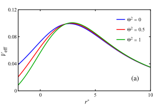
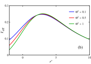
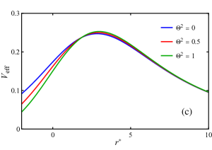
Figure 1: Effective potential for scalar field with $M=1$ in left panel $(a)$ for $l=1(m=\pm 1)$, in middle panel $(b)$ for $l=2$ $(m=\pm 1)$ and in the right panel $(c)$ for $l=2$ $(m=\pm 2)$ concerning different values of $\Theta^{2}$.

The influence of the NC parameter on the system can be observed through the behavior of the potentials. As the NC parameter increases, the potentials exhibit a higher maximum value. This indicates that the effective potential acts as a stronger barrier for the transmission of the field. Consequently, the NC effect is expected to have a prominent impact on QNMs and absorption cross section of the scalar field. The greybody factor, on the other hand, quantifies the probability of transmission through the effective potential barrier. To explore this further, we can utilize the effective potential to calculate the QNMs and the greybody factor in the following sections.

3 Non–commutative quasinormal modes

The QNMs represent the characteristic frequencies at which the scalar field oscillates, and its damping scale. By analyzing the QNMs, we can obtain information about the influence of NC parameter on the behavior of scalar field and its interaction with the effective potential. The determination of QNMs involves solving the wave equation in Eq. (2.20) that satisfies specific boundary conditions which require purely incoming waves at the event horizon and purely outgoing waves at infinity. However, due to the complexity of the equation, it cannot be solved analytically. Various analytical and numerical methods [61, 62, 63, 64, 65] have been proposed to find such frequencies. We choose three different methods in the following sections.

3.1 WKB method

The WKB approximation [66, 67, 68] gives the QNM by applying the following formula

$$\frac{{i(\omega_{n}^{2}-V_{0})}}{{\sqrt[\ ]{-2V^{\prime\prime}_{0}}}}+\sum\limits_{j=2}^{6}{{\Omega_{j}}=n+\frac{1}{2}},$$ (3.1)

Where $V_{0}$ and $V^{\prime\prime}_{0}$ is the value of effective potential and its respective second derivative of the effective potential with respect to $r^{*}$ at its maximum point and $\Omega_{j}$ are coming from WKB corrections [46, 47, 48]. In Tables. 1, 2 and 3, we present the outcome quasinormal frequencies. We consider two families of multipole numbers $l=1,2$ and their related monopoles which satisfy $(n\leq l)$, for $M=1$ and different values of $\Theta$. The case when $\Theta=0$ corresponds to the original Schwarzschild black hole as one should expect. Our observations reveal that increasing NC parameter leads to an increase in the real part of the QNMs, indicating a higher propagating frequency. Additionally, the imaginary part of the frequency follows the same trend as the $\Theta$ value increases, suggesting that higher values of NC parameter result in a lower damping timescale for the black hole.

Table 1: Quasinormal modes of scalar filed with third order WKB method for $M=1$, $l=1$, $m=1$, $n=0,1$ and various values of $\Theta^{2}$.

$\Theta^{2}$	$n=0$	$n=1$
0	0.29111 - 0.09800i	0.26221 - 0.30743i
0.2	0.29232 - 0.09940i	0.26513 - 0.31105i
0.4	0.29346 - 0.10075i	0.26754 - 0.31458i
0.6	0.29450 - 0.10199i	0.26927 - 0.31782i
0.8	0.29532 - 0.10272i	0.26855 - 0.31928i
1	0.29641 - 0.10434i	0.27144 - 0.32402i

Table 2: Quasinormal modes of scalar filed with third order WKB method for $M=1$, $l=2$, $m=1$, $n=0,1,2$ and various values of $\Theta^{2}$.

$\Theta^{2}$	$n=0$	$n=1$	$n=2$
0	0.48321 - 0.096805i	0.46319 - 0.29581i	0.43166 - 0.50343i
0.2	0.48443 - 0.098256i	0.46522 - 0.30000i	0.43509 - 0.50993i
0.4	0.48559 - 0.099694i	0.46699 - 0.30424i	0.43795 - 0.51669i
0.6	0.48670 - 0.101110i	0.46849 - 0.30848i	0.44023 - 0.52356i
0.8	0.48775 - 0.102470i	0.46963 - 0.31249i	0.44141 - 0.53004i
1	0.48877 - 0.103800i	0.47051 - 0.31640i	0.44188 - 0.53637i

Table 3: Quasinormal modes of scalar filed with third order WKB method for $M=1$, $l=2$, $m=2$, $n=0,1,2$ and various values of $\Theta^{2}$.

$\Theta^{2}$	$n=0$	$n=1$	$n=2$
0	0.48321 - 0.096805i	0.46319 - 0.29581i	0.43166 - 0.50343i
0.2	0.48465 - 0.098013i	0.46526 - 0.29937i	0.43490 - 0.50910i
0.4	0.48606 - 0.099226i	0.46714 - 0.30300i	0.43776 - 0.51499i
0.6	0.48741 - 0.100390i	0.46869 - 0.30642i	0.43956 - 0.52044i
0.8	0.48873 - 0.101530i	0.47001 - 0.30976i	0.44072 - 0.52579i
1	0.49002 - 0.102680i	0.47121 - 0.31316i	0.44164 - 0.53133i

3.2 Pösch–Teller and Rosen–Morse fitting method

Another method to solve the Eq. (2.20) is providing an approximation of the effective potential $V_{eff}$ to a solvable function. We choose the fitting approach to approximate it with the Pöschl–Teller (PT) [62, 63, 69, 70, 71] and Rosen–Morse (RM) functions [65, 72] for the calculation of QNMs. First, we utilize the Mathematica software to fit $V_{eff}$ with PT and RM functions. Fig. 2 demonstrate the $V_{eff}$ on which the PT and RM function are fitted, based on the least square method.

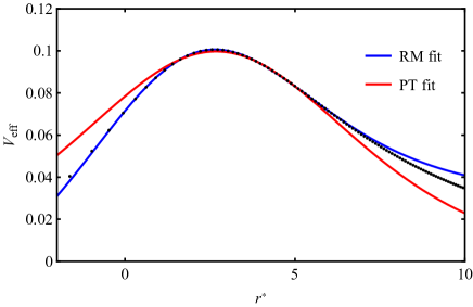
Figure 2: Fitting of $V_{eff}(r^{*})$ with Pösch–Teller and Rosen Morse function for scalar field, $M=1$, $l=1$ and $\Theta^{2}=0.5$. Dots show the effective potential points.

Next, it is approximated with PT function [73]

$$V_{eff}(r^{*})\sim V_{PT}=\frac{{{{V_{0}}}}}{{{{\cosh}^{2}}\gamma({r^{*}}-{{\bar{r}}^{*}})}}.$$ (3.2)

Here, ${V_{0}}$ and $\gamma$ are the height and the curvature of the effective potential $V_{eff}(r^{*})$ at its maximum point corresponding to ${\bar{r}}^{*}$, respectively. Then, solving Eq. (2.20) with the Pöschl–Teller approximation leads to the following equation for the calculation of QNMs [62]

$$\omega=i\gamma(n+\frac{1}{2})\pm\gamma\sqrt[\ ]{\frac{{{V_{0}}}}{{{\gamma^{2}}}}-\frac{1}{4}}.$$ (3.3)

The coefficients $V_{0}$ and $\gamma$ are found by fitting program, and the QNMs are calculated according to the Eq. (3.3).
Furthermore, the RM function [72] which has a correction term adding asymmetry to PT, can be considered in solving the Eq. (2.20) as approximation of the effective potential

$$V_{eff}(r^{*})\sim V_{RM}=\frac{{{{V_{0}}}}}{{{{\cosh}^{2}}\gamma({r^{*}}-{{\bar{r}}^{*}})}}+{V_{1}}\tanh\gamma({r^{*}}-{{\bar{r}}^{*}}).$$ (3.4)

The solution of wave function with this approach, yields the following expression [65]

$$\frac{{\sqrt[\ ]{{\omega^{2}}+{V_{1}}}+\sqrt[\ ]{{\omega^{2}}-{V_{1}}}}}{2}=i\gamma(n+\frac{1}{2})\pm\gamma\sqrt[\ ]{\frac{{{{V_{0}}}}}{{{\gamma^{2}}}}-\frac{1}{4}}.$$ (3.5)

in which $V_{1}$ is a new parameter added to PT function for better accuracy. The coefficients $V_{0}$, $V_{1}$ and $\gamma$ are obtained by fitting method via Mathematica software.

All results are represented in Table. 4. Both the real and imaginary part of QNMs for multipole number $l=1$ and $n=0$, are increasing with higher values of NC parameter.

Table 4: Comparison of QNMs of scalar field of NC Schwarzschild black hole obtained by using Pösch-Teller fitting, Rosen–Morse fitting and WKB method for $M=1$, $l=1$, $n=0$ and various values of parameter $\Theta$.

$\Theta^{2}$	PT fitting method	RM fitting method	WKB method
0	0.300322 - 0.090925i	0.296046 - 0.100235i	0.29111 - 0.09800i
0.2	0.300972 - 0.091393i	0.296157 - 0.101602i	0.29232 - 0.09940i
0.4	0.301622 - 0.091872i	0.296256 - 0.102960i	0.29346 - 0.10075i
0.6	0.302272 - 0.092345i	0.296344 - 0.104310i	0.29450 - 0.10199i
0.8	0.302924 - 0.092809i	0.296423 - 0.105652i	0.29532 - 0.10272i
1	0.303575 - 0.093290i	0.296491 - 0.106990i	0.29641 - 0.10434i

In essence, the results show that both fitting methods and WKB approximation align in the behavior of QNMs in the presence of NC spacetime.

4 Greybody factor and Absorption cross section

Greybody factors calculation are one of the crucial aspects of scattering issue due to the estimation of the portion of the initial quantum radiation in the vicinity of the event horizon reflected back and the amount of radiation which will reach the observer through the potential barrier. We shall take into account the radial wave Eq. (2.20) with the boundary conditions for incoming wave and outgoing wave as the following form [46, 48, 47]

$$\Psi_{\omega l}=\begin{cases}{{e^{-i\omega{r^{*}}}}+\mathrm{R}{e^{i\omega{r^{*}}}}}\quad\text{, if}\ {r^{*}}\to-\infty~{}(r\to{r_{h}})\\ {\mathrm{T}{e^{-i\omega{r^{*}}}}}\quad\quad\quad\quad\text{, if}\ {r^{*}}\to+\infty~{}(r\to\infty)\\ \end{cases}$$ (4.1)

where $\mathrm{R}$ and $\mathrm{T}$ are the reflection and transmission coefficients, respectively. The reflection coefficient is obtained by applying 3th order WKB method as [74, 75, 76, 77]

$$|\mathrm{R}|^{2}=\frac{1}{1+e^{-2i\pi\mathcal{K}}},$$ (4.2)

where

$$\mathcal{K}=\frac{i({\omega}^{2}-V_{0})}{\sqrt[\ ]{-2V^{\prime\prime}_{0}}}-\sum_{j=2}^{6}\Omega_{j}.$$ (4.3)

Here $\omega$ is purely real, $V_{0}$ and $V^{\prime\prime}_{0}$ is the effective potential in Eq. (2.21) and its second derivative at its maximum, $\Omega_{j}$ are coefficients associated with the effective potential. After finding the reflection coefficient by applying $|\mathrm{T}|^{2}+|\mathrm{R}|^{2}=1$, the transmission coefficient can be calculated [77, 78]

$$|\mathrm{T}|^{2}=\frac{1}{1+e^{+2i\pi\mathcal{K}}}.$$ (4.4)

As depicted in Fig. 3, increasing the value of $\Theta$ leads to a decrease in the greybody factors, indicating that a smaller fraction of the scalar field is able to penetrate the potential barrier. Additionally, in Fig. 1, it is evident that the height of the potential barrier increases with higher $\Theta$ values, resulting in a lower probability for particles to transmit through the barrier. Consequently, higher values of NC parameter results in a reduction in the greybody factor and a lower detection of incoming flow by the observer.

To investigate the probability for an outgoing wave to reach infinity, the Grey–body factors of the scalar field calculated using the third order WKB method are shown in Fig. 3 for various values of $\Theta$, specifically for multipole $l=1$.

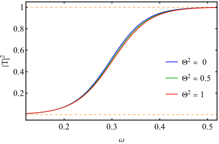
Figure 3: The greybody factors of the scalar field are computed using the third-order WKB method for $M=1$ and $l=1$ and $\Theta^{2}=0,05,1$.

As the figure shows, increasing the value of $\Theta$ yields a decrease in the Grey–body factors, indicating a smaller fraction of the scalar field is penetrating the potential barrier. In Fig. 1, for $l=1$ in panel $(a)$ and for $l=2$ in panel $(b)$ and $(c)$, it is obvious that the heights of the potential barriers go up with higher $\Theta$ values, which means the chance of particles to transmit through the barrier becomes lower. Therefore, higher values of non-commutativity leads to a reduction in the Grey–body factor and the detection of a lower fraction of incoming flow by the observer.

The partial absorption cross section can be determined by utilizing the transmission coefficient, which is defined as mentioned in Ref. [79, 45]

$${\sigma^{l}_{\mathrm{abs}}}=\frac{{\pi(2l+1)}}{{{{\omega}^{2}}}}{\left|{{\mathrm{T}_{l}}({\omega})}\right|^{2}},$$ (4.5)

where $l$ is the mode number and ${\omega}$ is the frequency

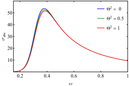
Figure 4: The partial absorption cross section of the scalar field are computed using the third order WKB method for $M=1$ and $l=1$ and various values of $\Theta^{2}$.

In Fig. 4, we have plotted the partial absorption cross section for $\Theta^{2}=0,0.5,1$. As observed, the absorption cross section decreases as the non-commutativity parameter increases. This observation aligns with the fact that the height of the effective potential barrier in Fig.1 increases with the non-commutativity parameter.

5 Non–commutative Null geodesics, Photonic radius and Shadows

Another important aspects that worth to be investigate, are the shadows and gravitational lensing in the vicinity of black hole [80, 81, 82, 83]. They take lots of attention specially after the pictures of $M87$ was taken by EHT in 2019 [84, 85, 86]. For examination of the black hole shadow radius and null geodesics, similarly what was used in Ref. [87], let us consider our diagonal metric, with $g_{ij}^{NC}$ parameters, in the general following form

$${g_{\mu\nu}}\mathrm{d}{x^{\mu}}\mathrm{d}{x^{\nu}}=-A(r)\mathrm{d}{t^{2}}+B(r)\mathrm{d}{r^{2}}+C(r,\theta)\mathrm{d}{\theta^{2}}+D(r){{\mathop{\rm\sin}\nolimits}^{2}}\theta\mathrm{d}{\varphi^{2}}.\\$$ (5.1)

By applying this form of our metric to the Lagrangian $L(x,\dot{x})=\frac{1}{2}({g_{\mu\nu}}{{\dot{x}}^{\mu}}{{\dot{x}}^{\nu}})$, it becomes

$$L(x,\dot{x})=\frac{1}{2}(-A(r){{\dot{t}}^{2}}+B(r){{\dot{r}}^{2}}+C(r,\theta){{\dot{\theta}}^{2}}+D(r){{\mathop{\rm\sin}\nolimits}^{2}}\theta{{\dot{\varphi}}^{2}}).$$ (5.2)

Now, we assume the geodesics in the equatorial plane $\theta=\frac{\pi}{2}$ which results in $\dot{\theta}=0$ and ${\mathop{\rm sin}\nolimits}\theta=1$. By writing the Euler–Lagrange equation for $t$ and $\phi$,

$$\frac{\mathrm{d}}{{\mathrm{d}\tau}}\left(\frac{{\partial L}}{{\partial{{\dot{x}}^{\mu}}}}\right)-\frac{{\partial L}}{{\partial{x^{\mu}}}}=0,$$ (5.3)

where we have two constant of motion called $E$ and $L$, which read

$$E=A(r)\dot{t}\quad\mathrm{and}\quad L=D(r)\dot{\varphi}.$$ (5.4)

For the sake of convenience, we shall denote $b=\frac{L}{E}$ as being an impact parameter. For light, ${g_{\mu\nu}}{{\dot{x}}^{\mu}}{{\dot{x}}^{\nu}}=0$, which means

$$-A(r){{\dot{t}}^{2}}+B(r){{\dot{r}}^{2}}+D(r){{\dot{\varphi}}^{2}}=0.$$ (5.5)

After applying Eq. (5.4) in Eq. (5.5), the trajectory of light in the equatorial plane can be calculated as

$$\frac{{{{\dot{r}}^{2}}}}{{{{\dot{\varphi}}^{2}}}}={\left(\frac{{\mathrm{d}r}}{{\mathrm{d}\varphi}}\right)^{2}}=\frac{{D(r)}}{{B(r)}}\left(\frac{{D(r)}}{{A(r)}}\frac{{{E^{2}}}}{{{L^{2}}}}-1\right).$$ (5.6)

Following Ref. [88, 89], we find out the formula for a shadow of an arbitrary spherically symmetric black hole. When the light ray reaches a minimum radius $r_{min}$ and goes out, $r_{min}$ is assumed as turning point which satisfies $\mathrm{d}r/\mathrm{d}\varphi=0$. If the function $h(r)$ is proposed as

$${h^{2}}(r)=\frac{{D(r)}}{{A(r)}},$$ (5.7)

so that Eq. (5.6) can be rewritten

$$\frac{{\mathrm{d}r}}{{\mathrm{d}\varphi}}=\pm\frac{{\sqrt[\ ]{D(r)}}}{{\sqrt[\ ]{B(r)}}}\sqrt[\ ]{\frac{{{h^{2}}(r)}}{{{h^{2}}(r_{min})}}-1}.$$ (5.8)

In this manner, the turning point has the following relation with the impact parameter

$$\frac{{{L^{2}}}}{{{E^{2}}}}=\frac{{D(r_{min})}}{{A(r_{min})}}=b^{2}\quad\rightarrow\quad h(r_{min})=b.$$ (5.9)

On the other hand, if we call the right hand of the Eq. (5.6) as ${\tilde{V}}_{eff}$, we can consider the following equation for the trajectory

$${\left(\frac{{\mathrm{d}r}}{{\mathrm{d}\varphi}}\right)^{2}}+{{\tilde{V}}_{eff}}=0,\quad\quad\text{where}\quad\quad{{\tilde{V}}_{eff}}=\frac{{{D(r)}}}{{{B(r)}}}\left({\frac{{{h^{2}}(r)}}{{{h^{2}}(r_{min})}}-1}\right).$$ (5.10)

Then, the circular orbits can then be determined by solving the expression below

$${{\tilde{V}}_{eff}}=\frac{{\mathrm{d}{{\tilde{V}}_{eff}}}}{{\mathrm{d}r}}=0.$$ (5.11)

Using above conditions, one can determine the radius of the photon sphere $r_{ph}$ by solving

$$\frac{\mathrm{d}}{{\mathrm{d}r}}{h^{2}}(r)=0\quad\rightarrow\quad{A^{\prime}(r)D(r)-D^{\prime}(r)A(r)}=0.$$ (5.12)

By taking into account that according to the main metric ($\mathrm{d}s^{2}=g_{ij}^{NC}\mathrm{d}x^{i}\mathrm{d}x^{j}$) in equatorial plane, we have

$$A(r) = -\left(1-\frac{{2M}}{r}\right)\left(1+\frac{{\alpha\left({8r-11\alpha}\right)}}{{16{r^{3}}\left({r-\alpha}\right)}}{\Theta^{2}}\right),$$ (5.13)

$$D(r) = {r^{2}}\left(1+\frac{{-\alpha(2r-\alpha)}}{{16{r^{3}}(r-\alpha)}}{\Theta^{2}}\right).$$ (5.14)

After some algebraic manipulations, the photonic radius becomes

$$\frac{-4\Theta^{2}M\left(2M^{2}-2Mr_{ph}+r_{ph}^{2}\right)-32r_{ph}^{3}(r_{ph}-2M)^{2}}{(2M-r_{ph})\left(16r_{ph}^{3}(r_{ph}-2M)+\Theta^{2}r_{ph}(r_{ph}-2M)+4\Theta^{2}M(M-r_{ph})\right)}+$$ (5.15)

$$\frac{8Mr_{ph}^{3}+4\Theta^{2}M(11M-3r_{ph})}{4r_{ph}^{3}(2M-r_{ph})+\Theta^{2}M(11M-4r_{ph})}=0.$$

The $r_{ph}$s are calculated for $M=1$ and various values of $\Theta$ to investigate the influence of non-commutativity on photonic spheres. When $\Theta$ equals to zero, the problem reduces to general Schwarzschild Black hole and we expect $r_{ph}$ and shadow radius to be $3M$ and $3\sqrt[\ ]{3}M$, respectively. In Table. 5, notably, it is observed that the photonic radius experience decrease when $\Theta$ goes from zero to 1. In Fig. 5, a light ray is shown which sent from the observer’s position at $ro$ into the past. The light ray angel with respect to the radial direction is named $\hat{\alpha}$ and it satisfies the following relation [88, 90].

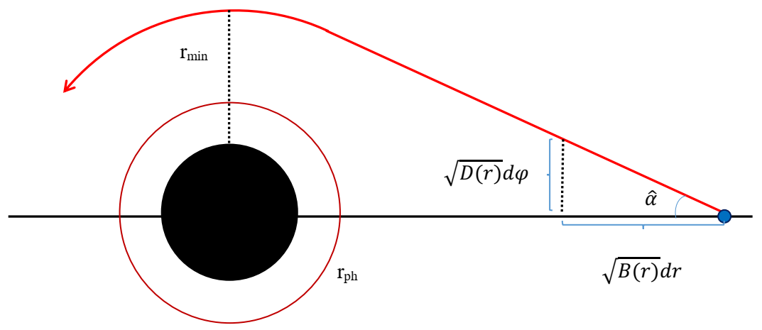
Figure 5: Schematic of light ray emitted from the observer’s position into the past under an angle $\hat{\alpha}$, $r_{ph}$ is the photon sphere radius and $r_{min}$ denotes the radius of the closest approach.

$$\cot\hat{\alpha}=\frac{{\sqrt[\ ]{{g_{rr}}}}}{{\sqrt[\ ]{{g_{\varphi\varphi}}}}}\frac{{\mathrm{d}r}}{{\mathrm{d}\varphi}}{|_{r=ro}}=\frac{{\sqrt[\ ]{B(r)}}}{{\sqrt[\ ]{D(r)}}}\frac{{\mathrm{d}r}}{{\mathrm{d}\varphi}}{|_{r=ro}}.$$ (5.16)

Now by taking into account the Eq. (5.8) for observer position we arrive at

$${\cot^{2}}\hat{\alpha}=\frac{{{h^{2}}(ro)}}{{{h^{2}}(r_{min})}}-1,\quad\longrightarrow\quad{\sin^{2}}\hat{\alpha}=\frac{{{h^{2}}(r_{min})}}{{{h^{2}}(ro)}}.$$ (5.17)

Therefore, the angular radius of the shadow can be determined by the assuming the condition $r_{min}\rightarrow r_{ph}$ in Eq. (5.17)

$${\sin^{2}}{\hat{\alpha}_{sh}}=\frac{{{h^{2}}({r_{ph}})}}{{{h^{2}}(ro)}}.$$ (5.18)

Then, considering the observer at a large distance, the shadow angel can be approximated by

$${\hat{\alpha}_{sh}}=\frac{{h({r_{ph}})}}{{h(ro)}}.$$ (5.19)

On the other hand, $\hat{\alpha}_{sh}$ approximately have the following relation with the shadow radius.

$${\hat{\alpha}_{sh}}=\frac{{{R_{sh}}}}{{ro}}.$$ (5.20)

Comparing Eq. (5.19) and (5.20) and considering the observer at infinity, leads to the next equation for shadow radius.

$${R_{sh}}=ro\frac{{h({r_{ph}})}}{{h(ro)}}=\sqrt[\ ]{\frac{{D({r_{ph}})}}{{A({r_{ph}})}}}=\frac{r_{ph}\sqrt[\ ]{4\left(\frac{\Theta^{2}M(r_{ph}-M)}{r_{ph}^{3}(2M-r_{ph})}+4\right)+\frac{\Theta^{2}}{r_{ph}^{2}}}}{2\sqrt[\ ]{\frac{4r_{ph}^{3}(r_{ph}-2M)+\Theta^{2}M(4r_{ph}-11M)}{r_{ph}^{4}}}}.$$ (5.21)

To investigate the effect of non–commutative parameter on the shadow radius, we applied Eq. 5.21 for various values of the $\Theta$. The results are represented in Table. 5.

Table 5: Photonic and shadow radius for $M=1$, $l=1$ and various values of $\Theta^{2}$

$\Theta^{2}$	0	0.2	0.4	0.6	0.8	1
$r_{ph}$	3.0000	2.9986	2.9972	2.9957	2.9943	2.9929
$R_{sh}$	5.1962	5.1853	5.1745	5.1637	5.1529	5.1422

For better visualization, we display an analysis of the shadows of our black hole for a range of $\Theta$ values with the help of stereo-graphic projection in the celestial coordinates $\eta$ and $\zeta$ [91] in Fig. 6.

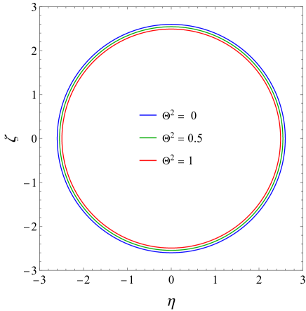
Figure 6: Shadow radius for $M=0.5$, $l=1$ and different NC parameter $\Theta^{2}=0,0.5,1$

It is evident that the shadow radius demonstrates a reduction as the non-commutative parameter increases, proving that $\Theta$ has a strong effect on the black hole shadow size.
Furthermore, the influence of the non-commutative parameter on the null geodesic curves is in our interest. By solving the Eq. 5.6 numerically, we verify the change of light trajectories for $M=0.5$ and different values of the non-commutative parameter in the Fig. 7. In the figures, we have a black disk that denotes the limit of the event horizon, the internal red dotted circle is the photonic radius, and the external green dotted circle is the shadow radius. Therefore, it is evident that the non-commutative parameter decreases the deflection effect of the black hole on the light beams. The black hole has a weaker influence on the light trajectory for bigger values of $\Theta$.

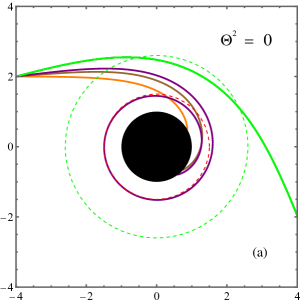
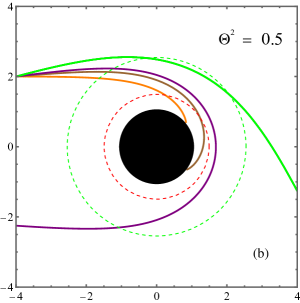
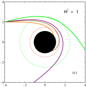
Figure 7: Null geodesics representation and in $(a)$ $\Theta^{2}=0$, in $(b)$ and $(c)$ the light trajectory with $\Theta^{2}=0.5$ and $\Theta^{2}=1$, respectively.

6 Conclusion

In this research, we investigated the influence of non–commutativity as a perturbation in the Schwarzschild black hole. Specifically, we examined the Klein–Gordon equation for a massless scalar field and obtained the effective potential affected by non–commutativity. To calculate the quasinormal mode for certain monopole numbers, we employed three methods. The WKB method and potential approximation using the Pösch–Teller and Rosen–Morse functions. By analyzing the real and imaginary parts of the these frequencies, we obtained a better understanding of how non–commutativity affects the propagation frequency of the scalar field and the damping scale of the black hole.

Our findings indicated that increasing the non–commutativity parameter led to higher scattering frequencies and damping timescales as well. Additionally, as it became stronger, the absorption cross section increased. Furthermore, we calculated the shadow radius, revealing that larger values of $\Theta$ resulted in smaller shadow radii. Lastly, our investigation of null–geodesics suggests that the NC spacetime reduce the gravitational lensing impact of the black hole on the trajectory of light.

References

- [1] Piero Nicolini. Noncommutative black holes, the final appeal to quantum gravity: a review. International Journal of Modern Physics A, 24(07):1229–1308, 2009.
- [2] Marija Dimitrijević Ćirić, Nikola Konjik, and Andjelo Samsarov. Noncommutative scalar quasinormal modes of the reissner–nordström black hole. Classical and Quantum Gravity, 35(17):175005, 2018.
- [3] Shao-Wen Wei, Peng Cheng, Yi Zhong, and Xiang-Nan Zhou. Shadow of noncommutative geometry inspired black hole. Journal of Cosmology and Astroparticle Physics, 2015(08):004, 2015.
- [4] Ali H Chamseddine, Alain Connes, and Walter D van Suijlekom. Noncommutativity and physics: a non-technical review. The European Physical Journal Special Topics, pages 1–8, 2023.
- [5] Nathan Seiberg and Edward Witten. String theory and noncommutative geometry. Journal of High Energy Physics, 1999(09):032, 1999.
- [6] Anais Smailagic and Euro Spallucci. Feynman path integral on the non-commutative plane. Journal of Physics A: Mathematical and General, 36(33):L467, 2003.
- [7] Anais Smailagic and Euro Spallucci. Uv divergence-free qft on noncommutative plane. Journal of Physics A: Mathematical and General, 36(39):L517, 2003.
- [8] Markus B Fröb, Albert Much, and Kyriakos Papadopoulos. Noncommutative geometry from perturbative quantum gravity. Physical Review D, 107(6):064041, 2023.
- [9] Piero Nicolini, Anais Smailagic, and Euro Spallucci. Noncommutative geometry inspired schwarzschild black hole. Physics Letters B, 632(4):547–551, 2006.
- [10] Leonardo Modesto and Piero Nicolini. Charged rotating noncommutative black holes. Physical Review D, 82(10):104035, 2010.
- [11] JC Lopez-Dominguez, O Obregon, M Sabido, and C Ramirez. Towards noncommutative quantum black holes. Physical Review D, 74(8):084024, 2006.
- [12] Robert B Mann and Piero Nicolini. Cosmological production of noncommutative black holes. Physical Review D, 84(6):064014, 2011.
- [13] T Kanazawa, G Lambiase, G Vilasi, and A Yoshioka. Noncommutative schwarzschild geometry and generalized uncertainty principle. The European Physical Journal C, 79(2):95, 2019.
- [14] Ashok Das, H Falomir, M Nieto, J Gamboa, and F Méndez. Aharonov-bohm effect in a class of noncommutative theories. Physical Review D, 84(4):045002, 2011.
- [15] G Zet, V Manta, and S Babeti. Desitter gauge theory of gravitation. International Journal of Modern Physics C, 14(01):41–48, 2003.
- [16] Ali H Chamseddine. Deforming einstein’s gravity. Physics Letters B, 504(1-2):33–37, 2001.
- [17] A. A. Araújo Filho, S Zare, PJ Porfírio, J Kříž, and H Hassanabadi. Thermodynamics and evaporation of a modified schwarzschild black hole in a non–commutative gauge theory. Physics Letters B, 838:137744, 2023.
- [18] Masud Chaichian, Anca Tureanu, and G Zet. Corrections to schwarzschild solution in noncommutative gauge theory of gravity. Physics Letters B, 660(5):573–578, 2008.
- [19] Kourosh Nozari and S Hamid Mehdipour. Hawking radiation as quantum tunneling from a noncommutative schwarzschild black hole. Classical and Quantum Gravity, 25(17):175015, 2008.
- [20] Sushant G Ghosh and Sunil D Maharaj. Noncommutative inspired black holes in regularized 4d einstein–gauss–bonnet theory. Physics of the Dark Universe, 31:100793, 2021.
- [21] MA Anacleto, FA Brito, SS Cruz, and E Passos. Noncommutative correction to the entropy of schwarzschild black hole with gup. International Journal of Modern Physics A, 36(03):2150028, 2021.
- [22] S Hamid Mehdipour. Hawking radiation as tunneling from a vaidya black hole in noncommutative gravity. Physical Review D, 81(12):124049, 2010.
- [23] Farook Rahaman, Sreya Karmakar, Indrani Karar, and Saibal Ray. Wormhole inspired by non-commutative geometry. Physics Letters B, 746:73–78, 2015.
- [24] I Arraut, Davide Batic, and Marek Nowakowski. A noncommutative model for a mini black hole. Classical and Quantum Gravity, 26(24):245006, 2009.
- [25] Rajes Ghosh, Nicola Franchini, Sebastian H Völkel, and Enrico Barausse. Quasi-normal modes of non-separable perturbation equations: the scalar non-kerr case. arXiv preprint arXiv:2303.00088, 2023.
- [26] N Heidari, H Hassanabadi, Kr̆íz̆, J, S Zare, PJ Porfírio, et al. Gravitational signatures of a non–commutative stable black hole. arXiv preprint arXiv:2305.06838, 2023.
- [27] Flavio Bombacigno, Fabio Moretti, Simon Boudet, and Gonzalo J Olmo. Landau damping for gravitational waves in parity-violating theories. Journal of Cosmology and Astroparticle Physics, 2023(02):009, 2023.
- [28] A. A Araújo Filho. Analysis of a regular black hole in verlinde’s gravity. arXiv preprint arXiv:2306.07226, 2023.
- [29] Simon Boudet, Flavio Bombacigno, Gonzalo J Olmo, and Paulo J Porfirio. Quasinormal modes of schwarzschild black holes in projective invariant chern-simons modified gravity. Journal of Cosmology and Astroparticle Physics, 2022(05):032, 2022.
- [30] H Hassanabadi, N Heidari, J Kríz, PJ Porfírio, S Zare, et al. Gravitational traces of bumblebee gravity in metric-affine formalism. arXiv preprint arXiv:2305.18871, 2023.
- [31] KM Amarilo, Ferreira MB Filho, A. A. Araújo Filho, and JAAS Reis. Gravitational waves effects in a lorentz-violating scenario. arXiv preprint arXiv:2307.10937, 2023.
- [32] Gaetano Lambiase, Reggie C Pantig, Dhruba Jyoti Gogoi, and Ali Övgün. Investigating the connection between generalized uncertainty principle and asymptotically safe gravity in black hole signatures through shadow and quasinormal modes. arXiv preprint arXiv:2304.00183, 2023.
- [33] Yi Yang, Dong Liu, Ali Övgün, Zheng-Wen Long, and Zhaoyi Xu. Probing hairy black holes caused by gravitational decoupling using quasinormal modes and greybody bounds. Physical Review D, 107(6):064042, 2023.
- [34] Benjamin P Abbott, R Abbott, TD Abbott, MR Abernathy, F Acernese, K Ackley, C Adams, T Adams, P Addesso, RX Adhikari, et al. Gw150914: The advanced ligo detectors in the era of first discoveries. Physical review letters, 116(13):131103, 2016.
- [35] Alex Abramovici, William E Althouse, Ronald WP Drever, Yekta Gürsel, Seiji Kawamura, Frederick J Raab, David Shoemaker, Lisa Sievers, Robert E Spero, Kip S Thorne, et al. Ligo: The laser interferometer gravitational-wave observatory. science, 256(5055):325–333, 1992.
- [36] Leonid P Grishchuk, VM Lipunov, Konstantin A Postnov, Mikhail E Prokhorov, and Bangalore Suryanarayana Sathyaprakash. Gravitational wave astronomy: in anticipation of first sources to be detected. Physics-Uspekhi, 44(1):1, 2001.
- [37] Sunny Vagnozzi, Rittick Roy, Yu-Dai Tsai, and Luca Visinelli. Horizon-scale tests of gravity theories and fundamental physics from the event horizon telescope image of sagittarius . arXiv preprint arXiv:2205.07787, 2022.
- [38] Reggie C Pantig and Ali Övgün. Testing dynamical torsion effects on the charged black hole’s shadow, deflection angle and greybody with m87* and sgr. a* from eht. Annals of Physics, 448:169197, 2023.
- [39] Emanuele Berti, Vitor Cardoso, and Andrei O Starinets. Quasinormal modes of black holes and black branes. Classical and Quantum Gravity, 26(16):163001, 2009.
- [40] RA Konoplya and Alexander Zhidenko. Quasinormal modes of black holes: From astrophysics to string theory. Reviews of Modern Physics, 83(3):793, 2011.
- [41] JAV Campos, MA Anacleto, FA Brito, and E Passos. Quasinormal modes and shadow of noncommutative black hole. Scientific Reports, 12(1):8516, 2022.
- [42] Grigoris Panotopoulos and Ángel Rincón. Quasinormal modes of five-dimensional black holes in non-commutative geometry. The European Physical Journal Plus, 135(1):33, 2020.
- [43] Jun Liang. Quasinormal modes of a noncommutative-geometry-inspired schwarzschild black hole. Chinese Physics Letters, 35(1):010401, 2018.
- [44] Rabin Banerjee, Bibhas Ranjan Majhi, and Saurav Samanta. Noncommutative black hole thermodynamics. Physical Review D, 77(12):124035, 2008.
- [45] MA Anacleto, FA Brito, JAV Campos, and E Passos. Absorption and scattering of a noncommutative black hole. Physics Letters B, 803:135334, 2020.
- [46] Sai Iyer and Clifford M Will. Black-hole normal modes: A wkb approach. i. foundations and application of a higher-order wkb analysis of potential-barrier scattering. Physical Review D, 35(12):3621, 1987.
- [47] RA Konoplya. Quasinormal behavior of the d-dimensional schwarzschild black hole and the higher order wkb approach. Physical Review D, 68(2):024018, 2003.
- [48] Bernard F Schutz and Clifford M Will. Black hole normal modes: a semianalytic approach. The Astrophysical Journal, 291:L33–L36, 1985.
- [49] Dhruba Jyoti Gogoi, Ali Övgün, and Durmuş Demir. Quasinormal modes and greybody factors of symmergent black hole. arXiv preprint arXiv:2306.09231, 2023.
- [50] Zeus S Moreira, Haroldo CD Lima Junior, Luís CB Crispino, and Carlos AR Herdeiro. Quasinormal modes of a holonomy corrected schwarzschild black hole. Physical Review D, 107(10):104016, 2023.
- [51] A Zhidenko. Quasi-normal modes of schwarzschild–de sitter black holes. Classical and Quantum Gravity, 21(1):273, 2003.
- [52] Mert Okyay and Ali Övgün. Nonlinear electrodynamics effects on the black hole shadow, deflection angle, quasinormal modes and greybody factors. Journal of Cosmology and Astroparticle Physics, 2022(01):009, 2022.
- [53] Ali Övgün, Reggie C Pantig, and Ángel Rincón. 4d scale-dependent schwarzschild-ads/ds black holes: study of shadow and weak deflection angle and greybody bounding. The European Physical Journal Plus, 138(3):192, 2023.
- [54] Reggie C Pantig, Leonardo Mastrototaro, Gaetano Lambiase, and Ali Övgün. Shadow, lensing, quasinormal modes, greybody bounds and neutrino propagation by dyonic modmax black holes. The European Physical Journal C, 82(12):1155, 2022.
- [55] M Sharif and Sehrish Iftikhar. Shadow of a charged rotating non-commutative black hole. The European Physical Journal C, 76:1–9, 2016.
- [56] Ashis Saha, Sai Madhav Modumudi, and Sunandan Gangopadhyay. Shadow of a noncommutative geometry inspired ayón beato garcía black hole. General Relativity and Gravitation, 50(8):103, 2018.
- [57] Eric Brown and Robert Mann. Instability of the noncommutative geometry inspired black hole. Physics Letters B, 694(4-5):440–445, 2011.
- [58] MA Anacleto, FA Brito, and E Passos. Gravitational aharonov–bohm effect due to noncommutative btz black hole. Physics Letters B, 743:184–188, 2015.
- [59] Che-Yu Chen, Hsu-Wen Chiang, and Jie-Shiun Tsao. Eikonal quasinormal modes and photon orbits of deformed schwarzschild black holes. Physical Review D, 106(4):044068, 2022.
- [60] Y Zhao, Yifu Cai, S Das, G Lambiase, EN Saridakis, and EC Vagenas. Quasinormal modes in noncommutative schwarzschild black holes. arXiv preprint arXiv:2301.09147, 2023.
- [61] Edward W Leaver. Solutions to a generalized spheroidal wave equation: Teukolsky’s equations in general relativity, and the two-center problem in molecular quantum mechanics. Journal of mathematical physics, 27(5):1238–1265, 1986.
- [62] Valeria Ferrari and Bahram Mashhoon. New approach to the quasinormal modes of a black hole. Physical Review D, 30(2):295, 1984.
- [63] Hans-Joachim Blome and Bahram Mashhoon. Quasi-normal oscillations of a schwarzschild black hole. Physics Letters A, 100(5):231–234, 1984.
- [64] Vitor Cardoso and Jose PS Lemos. Quasinormal modes of schwarzschild–anti-de sitter black holes: Electromagnetic and gravitational perturbations. Physical Review D, 64(8):084017, 2001.
- [65] N Heidari and H Hassanabadi. Investigation of the quasinormal modes of a schwarzschild black hole by a new generalized approach. Physics Letters B, 839:137814, 2023.
- [66] Jerzy Matyjasek and Michał Opala. Quasinormal modes of black holes: The improved semianalytic approach. Physical Review D, 96(2):024011, 2017.
- [67] Songbai Chen and Jiliang Jing. Quasinormal modes of a black hole surrounded by quintessence. Classical and Quantum Gravity, 22(21):4651, 2005.
- [68] Roberto Avalos and Ernesto Contreras. Quasi normal modes of hairy black holes at higher-order wkb approach. The European Physical Journal C, 83(2):155, 2023.
- [69] Supakchai Ponglertsakul and Bogeun Gwak. Massive scalar perturbations on myers-perry–de sitter black holes with a single rotation. The European Physical Journal C, 80:1–17, 2020.
- [70] Ramin G Daghigh, Michael D Green, and Jodin C Morey. Significance of black hole quasinormal modes: A closer look. Physical Review D, 101(10):104009, 2020.
- [71] Ronit Karmakar, Dhruba Jyoti Gogoi, and Umananda Dev Goswami. Quasinormal modes and thermodynamic properties of gup-corrected schwarzschild black hole surrounded by quintessence. International Journal of Modern Physics A, 37(28n29):2250180, 2022.
- [72] N Rosen and Philip M Morse. On the vibrations of polyatomic molecules. Physical Review, 42(2):210, 1932.
- [73] Gertrud Pöschl and Edward Teller. Bemerkungen zur quantenmechanik des anharmonischen oszillators. Zeitschrift für Physik, 83(3-4):143–151, 1933.
- [74] Sharmanthie Fernando. Bardeen–de Sitter black holes. Int. J. Mod. Phys. D, 26(07):1750071, 2017.
- [75] Marcos A Anacleto, JAV Campos, Francisco A Brito, and E Passos. Quasinormal modes and shadow of a schwarzschild black hole with gup. Annals of Physics, 434:168662, 2021.
- [76] Bobir Toshmatov, Ahmadjon Abdujabbarov, Zdeněk Stuchlík, and Bobomurat Ahmedov. Quasinormal modes of test fields around regular black holes. Physical Review D, 91(8):083008, 2015.
- [77] Roman A Konoplya and Antonina F Zinhailo. Grey-body factors and hawking radiation of black holes in 4d einstein-gauss-bonnet gravity. Physics Letters B, 810:135793, 2020.
- [78] Bobir Toshmatov, Zdeněk Stuchlík, Jan Schee, and Bobomurat Ahmedov. Quasinormal frequencies of black hole in the braneworld. Physical Review D, 93(12):124017, 2016.
- [79] Luís CB Crispino, Sam R Dolan, and Ednilton S Oliveira. Scattering of massless scalar waves by reissner-nordström black holes. Physical Review D, 79(6):064022, 2009.
- [80] Xiao-Xiong Zeng, Guo-Ping Li, and Ke-Jian He. The shadows and observational appearance of a noncommutative black hole surrounded by various profiles of accretions. Nuclear Physics B, 974:115639, 2022.
- [81] Bilel Hamil and BC Lütfüoğlu. Thermodynamics and shadows of quantum-corrected reissner–nordström black hole surrounded by quintessence. Physics of the Dark Universe, 42:101293, 2023.
- [82] MA Anacleto, FA Brito, JAV Campos, and E Passos. Absorption, scattering and shadow by a noncommutative black hole with global monopole. The European Physical Journal C, 83(4):298, 2023.
- [83] Zening Yan, Xiaoji Zhang, Maoyuan Wan, and Chen Wu. Shadows and quasinormal modes of a charged non-commutative black hole by different methods. The European Physical Journal Plus, 138(5):1–14, 2023.
- [84] David Ball, Chi-kwan Chan, Pierre Christian, Buell T Jannuzi, Junhan Kim, Daniel P Marrone, Lia Medeiros, Feryal Ozel, Dimitrios Psaltis, Mel Rose, et al. First m87 event horizon telescope results. i. the shadow of the supermassive black hole. The Astrophysical Journal Letters, 2019.
- [85] Samuel E Gralla. Can the eht m87 results be used to test general relativity. Physical Review D, 103(2):024023, 2021.
- [86] Kazunori Akiyama, Antxon Alberdi, Walter Alef, Keiichi Asada, Rebecca Azulay, Anne-Kathrin Baczko, David Ball, Mislav Baloković, John Barrett, Dan Bintley, et al. First m87 event horizon telescope results. v. physical origin of the asymmetric ring. The Astrophysical Journal Letters, 875(1):L5, 2019.
- [87] Davide Batic, S Nelson, and M Nowakowski. Light on curved backgrounds. Physical Review D, 91(10):104015, 2015.
- [88] Volker Perlick, Oleg Yu Tsupko, and Gennady S Bisnovatyi-Kogan. Influence of a plasma on the shadow of a spherically symmetric black hole. Physical Review D, 92(10):104031, 2015.
- [89] RA Konoplya. Shadow of a black hole surrounded by dark matter. Physics Letters B, 795:1–6, 2019.
- [90] Volker Perlick and Oleg Yu Tsupko. Calculating black hole shadows: Review of analytical studies. Physics Reports, 947:1–39, 2022.
- [91] Balendra Pratap Singh and Sushant G Ghosh. Shadow of schwarzschild–tangherlini black holes. Annals of Physics, 395:127–137, 2018.