Spatialyze: A Geospatial Video Analytics System with Spatial-Aware Optimizations

Abstract.

Videos that are shot using commodity hardware such as phones and surveillance cameras record various metadata such as time and location. We encounter such geospatial videos on a daily basis and such videos have been growing in volume significantly. Yet, we do not have data management systems that allow users to interact with such data effectively.

In this paper, we describe Spatialyze, a new framework for end-to-end querying of geospatial videos. Spatialyze comes with a domain-specific language where users can construct geospatial video analytic workflows using a 3-step, declarative, build-filter-observe paradigm. Internally, Spatialyze leverages the declarative nature of such workflows, the temporal-spatial metadata stored with videos, and physical behavior of real-world objects to optimize the execution of workflows. Our results using real-world videos and workflows show that Spatialyze can reduce execution time by up to 5.3$\times$, while maintaining up to 97.1% accuracy compared to unoptimized execution.

1. Introduction

Geospatial videos are videos in which the location and time that they are shot are known. From surveillance footage, autonomous vehicle cameras to police body cameras, such videos are prevalent in our daily lives. While the volume of such data has grown tremendously (Wright, 2023; Sparks, 2023), we still lack end-to-end systems that can process and query such data effectively. The rise of machine learning (ML) in recent years has aggravated this issue, with the latest deep learning models capable of carrying out various computer vision tasks, such as object detection (Girshick et al., 2014; Jocher et al., 2022; Girshick, 2015; Redmon and Farhadi, 2018; Ren et al., 2016), multi-objects tracking (Bewley et al., 2016; Du et al., 2023; Wojke et al., 2017; Broström, 2022), image depth estimation (Godard et al., 2019), etc.

All these trends have made geospatial video analytics computationally intensive. For instance, a $2299 Nvidia T4 GPU takes 34 seconds on average to execute a simple workflow of object detection, tracking, and image depth estimation on a 20-second 12-fps video. Modern autonomous driving datasets, such as nuScenes (Caesar et al., 2019), contain 6000 such videos. Running the workflow mentioned above will take 3 full days to run on the entire dataset.

To make matters worse, the lack of programming frameworks and data management systems for geospatial videos has made it challenging for end users to specify their workflows, let alone running them efficiently. Consider a data journalist writing an article on police misconduct and would like to examine the footage collected on police body cameras to look for specific behavior, e.g., police chasing after a suspect. Given today’s technology, they will either need to watch all the footage themself or string together various ML models for video analytics (Kang et al., 2017; Bastani et al., 2020; Bastani and Madden, 2022; Xu et al., 2022) and video processing libraries (e.g., FFmpeg (Tomar, 2006), OpenCV (Bradski, 2000)) to construct their workflow. Sadly, the former is simply infeasible given the amount of video data collected, while the latter requires deep programming expertise that most users do not possess.

We see an opportunity to build a programming framework that bridges video processing and geospatial video analytics. Specifically, given that users constructing workflows on geospatial videos are typically interested in the time and location where such videos are taken, we should exploit the metadata stored in geospatial videos to optimize such workflows. For instance, a car is at $(1810.39,1221.71,0.90)$ in the Boston Seaport map, which is at an intersection, at 2:33:59.112 PM of September 18, 2018. Each object inside a video captures a real-world object; therefore, this object also inherits physical behavior that its real-world counterpart would have had. For example, when users look for a car at a road intersection, we know that a road intersection need to be visible in the video frames that the car of interest is visible; therefore, video frames without a visible road intersection, determined with geospatial metadata, need not be processed with expensive ML functions. We leverage this already existing geospatial metadata, the inherited physical behaviors, and users’ queries to speed up video processing.

To leverage this insight, we present Spatialyze, a system for geospatial video analytics. To make it easy for users to specify their geospatial video workflows, Spatialyze comes with a conceptual data model where users create and ingest videos into a “world,” and users interact with the world by specifying objects (e.g., cars) and scenarios (e.g., cars crossing an intersection) of interest via Spatialyze’s domain-specific language (DSL) embedded in Python called S-FLow. Spatialyze then efficiently executes the workflow by leveraging various spatial-aware optimization techniques that make use of existing geospatial metadata and assumptions based on inherited physical behavior of objects in the videos. For instance, Spatialyze’s Road Visibility Pruner uses road’s visibility as a proxy for objects’ visibility to prune out video frames. The Object Type Pruner then prunes out objects that are not of interest to the users’ workflow. Spatialyze’s 0pt speeds up object 3D location estimation by replacing a computationally expensive ML-based approach with a geometry-based approach. Finally, the Exit Frame Sampler prunes out unnecessary video frames based on the inherited physical behavior of vehicles and traffic rules. Spatialyze’s optimizations are all driven by various geospatial metadata and real-world physical behavior, with a goal to reduce the number of video frames to be processed and ML operations to be invoked, thus speeding up video processing runtime.

As we are unaware of end-to-end frameworks for geospatial video processing, we evaluate the different parts of Spatialyze against state-of-the-art video analytic tools (EVA (Xu et al., 2022) and OTIF (Xu et al., 2022)), and a geospatial data analytic tool (nuScenes devkit (Caesar et al., 2019)) on different geospatial video workflows. The results show that we are 7-68$\times$ faster than EVA in geospatial object detection workflow, 1.11-1.27$\times$ faster than OTIF in object tracking, and 117-716$\times$ faster than nuScenes in geospatial data analytics. We also evaluate each of our optimization techniques by executing each of the queries with and without each of the techniques. The results show that our optimization techniques achieve 2.5-5.3$\times$ speed up with 83.4-97.1% accuracy on 3D object tracking.

In sum, we make following contributions:

• In Sec. 4, we present a conceptual data model and a DSL (S-FLow) for geospatial video analytics. Using S-FLow, users construct their workflows simply by following our build-filter-observe paradigm to interact with their videos.

• In Sec. 6, we develop four optimization techniques that leverage geospatial metadata embedded in videos and inherited physical behavior of objects to speed up geospatial video processing in Spatialyze’s geospatial video analytic workflow.

• In Sec. 7, we implemented our techniques in Spatialyze and evaluated it against other state-of-the-art video processing techniques as well as ablation studies, using real-world videos from nuScenes (Caesar et al., 2019).

2. Related Work

Geospatial Video Analytics

Recent use cases for querying geospatial video data (autonomous driving (Kim et al., 2021b), surveillance (Griffin and Miller, 2008), traffic analysis (Gloudemans and Work, 2021), and transshipment activities (McDonald et al., 2021; Park et al., 2020)) have driven attention to building geospatial DBMSs for data storage and retrieval. VisualWorldDB (Haynes et al., 2020) allows users to ingest video data from diverse sources and make them queryable as a single multidimensional object. It optimizes query execution by jointly compressing overlapping videos and reusing results from them. Apperception (Ge et al., 2021) provides a Python API for users to input geospatial videos and organizes them into a four-dimensional data model. Users can then use its API to query video data. While such data models are designed to avoid repeating expensive video operations (e.g., model inference), Spatialyze provides a concise end-to-end workflow interface for geospatial video analytics that automatically analyzes the workflow then applies optimization techniques to speed up such video operations. In addition, Spatialyze supports multiple operations that integrate geospatial metadata as contexts for objects in videos.

Video Processing

Researchers have proposed techniques to efficiently detect, track, and estimate 3D locations of objects from videos. Monodepth2 (Godard et al., 2019) estimates per-pixel image depth data using only monocular videos. EVA (Xu et al., 2022) identifies, materializes, and reuses expensive user-defined functions (UDF) on videos for exploratory video analytics with multiple refined and reused queries. However, EVA’s optimization techniques are aimed at scenarios where multiple queries use a high degree of overlapping UDFs. OTIF (Bastani and Madden, 2022) is a general-purpose object tracking algorithm. It uses a segmentation proxy model to determine if frames or regions of frames contain objects that need to be processed with an object detector, along with a recurrent reduced-rate tracking method that speed up tracking by reducing frame rate. Complexer-YOLO (Simon et al., 2019) and EagerMOT (Kim et al., 2021a) propose one-stop machine learning models for efficiently tracking 3D objects using LiDAR data, which is not always available compared to cameras and GPS sensors. In addition, 3D sensing data is large. For instance, storing 850 20-second-long scenes of LiDAR sensor data in nuScenes requires 162 GB, while videos of the same scenes only take up 92 GB. Spatialyze overcomes this limitation by not requiring such information to process geospatial workflows, and instead readily available geospatial metadata to optimize user workflows. In addition, one of our optimization techniques estimates objects’ 3D location 192$\times$ faster than the approach that uses Monodepth2 on average.

3. Usage Scenario

In this section, we give an overview of Spatialyze using an example. Suppose a data journalist is interested in investigating autonomous driving vehicle (AV) footage reports. Specifically, they want to find snippets of videos where other vehicles crash into the drivers’ vehicle at a road intersection.

Naively, the data journalist would watch all the videos individually, identify parts of videos that are relevant to further analyze. However, this process is extremely slow, tedious, and error-prone due to the number of videos to watch.

Instead, the journalist can use geospatial video data analytic tools to help them reduce the workload and speed up the processes. Besides video footage, they may also have access to camera movement information of each video and road network information of the city where the videos are shot. With Spatialyze, they can construct an analytic workflow with using S-FLow’s 3-step paradigm as shown in Fig. 1 to:

1. Build a world, by integrating the video data with the geospatial metadata (road network and camera configurations).

2. Filter for the video parts of interest, by describing relationships between objects (humans, cars, trucks) and their surrounding geospatial environment (road, lane, intersection).

3. Observe the filtered video parts, in this case, by saving all the filtered video parts into video files for further examination.

Build a world

In line LABEL:line:world, the users start by initializing a world. A world represents a geospatial virtual environment; a concept that to be discussed in Sec. 4. Line LABEL:line:road then shows initialization of the world by loading roadNetwork data, which represents a set of road segments in the Boston Seaport area. Lines LABEL:line:gsvideo-LABEL:line:end-build then load videos from files along with their camera configurations. Each camera configuration file contains camera locations, rotations, and intrinsics (Zhang, 2014) over time. Then, they associate each video with its corresponding camera configurations, creating a geospatial video, and adding it into the world. Finally, in line LABEL:line:end-build, they have constructed a data-rich world with video cameras, and road segments, all related spatially and temporally.

Filter for the video parts of interest

From the data journalist’s perspective, objects and their trackings from each video added to the world are readily querable, and users can interact with through object(). Here, our journalist wants to find snippets of video with the characteristics mentioned earlier. They can do so by adding a filter to the world to only include objects that match the provided predicates. In line LABEL:line:pred-type, the objects of interest need to be cars or trucks. In line LABEL:line:pred-distance, the objects of interest is within 50 meters of the camera. In line LABEL:line:pred-contain, they specify the objects of interest to be those at an intersection, and in line LABEL:line:pred-heading, the objects are required to be moving towards the camera. After filter is executed at line LABEL:line:pred-heading, the world will contain only cars or trucks on intersections that are moving towards the camera, as desired.

Observe the filtered video parts

After our journalist applies the filter, the world contains much fewer objects compared to when it was initialized. In line LABEL:line:observe, they call saveVideos(). Spatialyze does not save all the videos that the data journalists initially input. Instead, it saves only snippets of videos containing objects that currently exist in the world. The total length of the video snippets combined is now much shorter than that of the original. Therefore, our journalist now spends less time watching videos as they only need to watch the relevant ones, with objects of interest highlighted. As shown, S-FLow provides a declarative interface where users do not specify “how” to find the video snippets of interest; instead, they only need to describe “what” their video snippets of interest look like, and Spatialyze will optimize accordingly.

⬇

world = World() # OR World(detect=CstmDetector, track=CstmTracker) $\label{line:world}$

roadNetwork = RoadNetwork(’road-network/boston-seaport/’)!$\label{line:road-init}$!

world.addGeogConstructs(roadNetwork) !$\label{line:road}$!

world.addVideo(GeospatialVideo(Video(’v0.mp4’), Camera(’c0.json’))) !$\label{line:gsvideo}$!

world.addVideo(GeospatialVideo(Video(’v1.mp4’), Camera(’c1.json’))) !$\label{line:end-build}$!

obj, cam, intersection = (world.object(), world.camera(), !$\label{line:object}$!

world.geogConstruct(type=’intersection’))

world.filter( !$\label{line:filter}$!

((obj.type == ’car’) | (obj.type == ’truck’)) & !$\label{line:pred-type}$!

(distance(obj, cam) < 50) & !$\label{line:pred-distance}$!

contains(intersection, obj) & !$\label{line:pred-contain}$!

headingDiff(obj, cam, between=[135, 225]) ) !$\label{line:pred-heading}$!

world.saveVideos(’output_videos/’, addBoundingBoxes=True) !$\label{line:observe}$!

Figure 1. Geospatial Video Analytic Workflow with Spatialyze

From the users’ perspective, Spatialyze automatically tracks objects from videos, right after each of them is added to the world. Hence, they can filter the world using these tracked objects. Internally, however, Spatialyze does not execute any part of the workflow until users call saveVideos(). In Fig. 1, Spatialyze internally only records an execution graph when lines LABEL:line:road-LABEL:line:pred-heading are executed. Only at line LABEL:line:observe, after the user calls saveVideos() does Spatialyze actually trigger planning and execute of the entire workflow. Deferring executions this way allows Spatialyze to analyze the entire workflow for efficient execution.

We next discuss S-FLow in detail and how it optimizes workflow execution by leveraging video metadata and physical behavior of real-world objects.

4. Constructing Geospatial Video Analytic Workflows

Spatialyze comes with a domain-specific language (DSL) called S-FLow embedded in python for users to construct their geospatial video data workflow. In this section we describe S-FLow with Spatialyze’s conceptual data model.

4.1. Conceptual Data Model

To analyze videos in a general purpose programming language, users need to manually extract and manipulate objects’ bounding box from individual video frames. To analyze geospatial metadata along with the video, users need to manually join the bounding boxes spatially with the geospatial metadata. These processes are very tedious. Hence, we design a higher-level abstraction for users to interact with their geospatial video data. Spatialyze’s data model serves as the programming model for users interact with their geospatial video data. The data model comprises of 4 concepts: 1) World, 2) Geographic Constructs, 3) Movable Objects, and 4) Cameras. We discuss each of them below.

4.1.1. World

As discussed in Sec. 3 and in line LABEL:line:world of Fig. 1, users construct a World as a first step of using Spatialyze. Inspired by VisualWorldDB (Haynes et al., 2020), a World represents a geospatial virtual environment. It is the outer-most building-block that contains Geographic Constructs, Movable Objects, and Cameras. Coexisting in the same environment, each of Geographic Constructs, Movable Objects, and Cameras have spatial relationships between each other. This shared spatial relationship along with S-FLow enable users to expressively and concisely describe the characteristics of the videos of interest. A World also reflects the physical world; therefore, Movable Objects inside are expected to behave the same ways as the ones in the physical world. For example, a car is on the ground, follows their lanes, and travels at the speed limit. We refer to these phenomena as inherited physical behaviors of Movable Objects. We will discuss how Spatialyze leverage these physical behaviors to optimize video processing in Sec. 6.

4.1.2. Geographic Constructs

Each World has a set of Geographic Constructs; each Geographic Construct has a spatial property that defines its area, represented as a polygon. It also has non-spatial properties including construct ID and construct type. We model each Geographic Construct as $(cid,\allowbreak type,\allowbreak((x_{0},y_{0}),\allowbreak(x_{1},y_{1}),\allowbreak...))$ where $cid$ is its identifier; $type$ is the construct type, such as road section, lane, or intersection; and, each $x_{i},y_{i}$ is a vertex of the polygon that represents the area of the construct.

4.1.3. Movable Objects

Besides static properties like Geographic Constructs, a World may contain multiple Movable Objects. Being movable, they each have a spatiotemporal property, i.e., its location at a given time. They also have non-spatial properties including object ID and object type that does not change throughout the object’s life-span. For example, a Movable Object with object type of “car” will always be a “car.” Spatialyze models each Movable Object as $(oid,type,((l_{0},t_{0}),\allowbreak(l_{1},t_{1}),...))$, where $oid$ is its identifier; $type$ is the object type, such as car, truck, or human; and, $l_{i}=(x_{i},y_{i},z_{i})$ is its location at time $t_{i}$.

4.1.4. Camera

As a special type of Movable Object, a Camera represents a camera where videos are captured. A Camera has spatio-temporal properties (Zhang, 2014). We model each Camera as $(cid,((l_{0},\allowbreak r_{0},\allowbreak it_{0},\allowbreak t_{0}),\allowbreak(l_{1},\allowbreak r_{1},it_{1},\allowbreak t_{1}),...))$, where $cid$ is the camera’s ID. At time $t_{i}$, $l_{i}=(x_{i},y_{i},z_{i})$ is its location; $r_{i}$ is its 3D rotation, defined as a quaternion (Kuipers, 1999); and, $it_{i}$ is its intrinsic (Zhang, 2014; Anwar, 2022).

We intentionally do not include “video” as a part of our conceptual data model. A video itself does not have any geospatial property, so it does not exist in a World. Similarly, none of the objects tracked in the video exists initially in the World. Internally, only after we bind the video with a Camera will the video gain geospatial properties from the Camera, and the video becomes a part of the Camera. Objects tracked in the video also gain their geospatial properties, as a result of the binding. Spatialyze derives the objects’ geospatial locations, by combining their 2 dimensional bounding boxes and Camera’s geospatial information. An object tracked that gain geospatial properties then becomes a Movable Object in the World.

4.2. S-FLow

We design S-FLow based on the data model presented in Sec. 4.1, where users interact and manipulate geospatial objects via Geographic Constructs, Movable Objects, and Cameras rather than video frames. S-FLow’s language constructs consists of functions that operate on World, RoadNetwork, and GeospatialVideo. Users compose such functions to construct geospatial video analytics workflows.

4.2.1. Camera

Lines LABEL:line:gsvideo-LABEL:line:end-build of Fig. 1 defines a Camera as discussed in in Sec. 4.1.4. Users initialize a Camera from a list or a file with a JSON (Pezoa et al., 2016) specification, where the $i$-th element of the list is a dictionary with 4 fields: translation, rotation, intrinsic, and timestamp. They correspond to $l_{i}$, $r_{i}$, $it_{i}$, and $t_{i}$, as defined in Sec. 4.1.4.

4.2.2. GeospatialVideo

A GeospatialVideo is a video enhanced with geospatial metadata. A Video (lines LABEL:line:gsvideo-LABEL:line:end-build of Fig. 1) by itself contains a list of consecutive RGB images where each image represents a frame of the video. Such video exists spatially in the World after its Video object is bound to a Camera to obtain its spatial properties, where each frame $i$ is an image taken from a camera at location $l_{i}$, rotation $r_{i}$, intrinsic $it_{i}$, and captured at time $t_{i}$. The objects in each frame obtains its geospatial properties after its track is inferred from GeospatialVideo. These tracked objects then become Movable Objects as defined in Sec. 4.1.3.

4.2.3. RoadNetwork

A RoadNetwork is a collection of road segments. Each road segment is a Geographic Construct as defined in Sec. 4.1.2. Besides being a Geographic Construct, a road segment stores its segment heading, which indicate traffic headings in that road segment. A road segment have multiple segment headings (curve lane) or no segment heading at all (intersection). Road segments in the RoadNetwork dataset that we use have following road types: roadsection, intersection, lane, and lanegroup. In S-FLow, we initialize a RoadNetwork by loading from a directory containing files of road network from each type. These road network information is accessible and often provided with AV video datasets (Fritsch et al., 2013; Caesar et al., 2019).

4.2.4. World

Each language construct we introduced so far represents users’ data. Bringing the concept of World described in Sec. 4.1.1 into our DSL, users interact with all of their video data through Geographic Construct, Movable Objects, and Camera that exists in a World. In a Spatialyze workflow, users interact with the World with this 3-step paradigm: build, filter, and observe. Users start from building a World by adding videos and geospatial metadata. Once built, users filter the World to only contain their objects of interest. Finally, users observe the remaining objects through annotated videos outputs.

Build. A World is initially empty. Users add RoadNetwork using addGeogContructs(), following by adding GeospatialVideo via addVideo(). At this point of the workflow, the World contains Geographic Constructs, and Cameras.

Filter. Users then construct predicates to filter objects of their interest. As discussed in Sec. 3, Spatialyze has not extracted detections and trackings of objects from the videos yet at this point. Nonetheless, Spatialyze provides an interface for users to interact with these objects as if they are already exist. For instance, object() refers to an arbitrary Movable Object in the World that is referenced in the predicate. Calling multiple object() gives users multiple arbitrary Movable Objects to use in the predicate. For the information that are already exist, camera() refers to an arbitrary Camera. Similarly, geoConstruct(type=...) refers to a Geographic Construct of a certain type. Users can construct a predicate on a Movable Object’s or Camera’s properties. For example, obj.type=="car" is a predicate that restricts obj to only be a car. They can also construct a predicate involving multiple Movable Object, Camera, or Geographic Construct, using our provided helper functions. For instance, contains(intersection,obj) determines if intersection as a polygon contains obj as a point. headingDiff(obj,cam,between=[135,255]) determines if the difference of the heading of obj and the heading of cam is between 135 and 255 degrees. In addition, we provide more helper functions and an interface for users to define their own helper functions. Finally, users can chain the filter or use Boolean operators to combine predicates.

Observe. After filtering their desired Movable Objects, users observe the filtered World, using one of the following 2 observer functions. First, they can observe the World by watching through snippets of the users’ own input videos. Using saveVideos(file, addBoundingBoxes) function, Spatialyze saves all the video snippets that contains the Movable Objects of interest to a file, where addBoundingBoxes is Boolean flag that indicate whether the bounding box of each Movable Objects should be shown. Second, they can observe the World by getting the Movable Object directly. Using getObjects(), Spatialyze returns a list of Movable Objects and their trajectories.

Customize Inference Functions

By default, Spatialyze uses YOLOv5 (Jocher et al., 2022) for object detection and StrongSORT (Du et al., 2023) for object tracking. Spatialyze also supports using UDFs for object detection or tracking, as shown commented in line LABEL:line:world of Fig. 1.

5. Workflow Execution

From users’ view, Spatialyze simply filters objects in the World after they call filter(). Then, they can observe the filtered objects afterwards, using one of the observer functions described in Sec. 4.2.4. Internally, Spatialyze only performs video processing to detect objects and compute tracks for them as needed given the workflow. For example, in line LABEL:line:pred-heading of Fig. 1, the user filters on objects’ moving directions. Executing this requires computing the trajectory of objects in the given videos to compute their directions. Given a S-FLow workflow, the goal of Spatialyze is to understand the users’ workflow, recognize and execute the video processing steps that are needed for user’s filter predicates, and return the Movable Objects that satisfy users’ filters.

In Sec. 4, we discuss a high-level interface for Spatialyze that allows users to declaratively construct their geospatial video analytic workflows. Users follow the build-filter-observe pattern without knowing when the actual execution happens. Internally, all execution happens when the users observe the world. In this section, we discuss the benefits of deferred execution and how Spatialyze generates execution plans for a workflow.

5.1. Deferred Execution

Video processing with ML functions take time. If Spatialyze performs them immediately when users add data, Spatialyze has to blindly perform the processing for the whole video without seeing the entire workflow. As a result, it could miss potential optimizations on processing the video. To resolve this, Spatialyze defers expensive execution until users need to observe the World. This way, Spatialyze gets to see the entire workflow before execution so that it can be optimized.

5.2. Workflow Execution Stages

Once users observe a World, Spatialyze starts executing users’ workflow in 4 stages sequentially: (1) Data Integrator, (2) Video Processor, (3) Movable Objects Query Engine, and (4) Output Composer. Each stage performs a sequence of steps based on the workflow. Fig. 2 shows how Spatialyze executes a user’s workflow in these 4 stages.

5.2.1. Data Integrator

In this stage, Spatialyze processes all the input data (video and geospatial metadata) from when the user Builds their World. Spatialyze processes the Geographic Constructs by creating tables in a geospatial metadata store (our implementation uses MobilityDB (Zimányi et al., 2020)) to store the RoadNetwork and create spatial indexing for every Geographic Construct. Then, it joins each Video and its corresponding Camera frame-by-frame, by their timestamp or frame number. The results of these joins are GeospatialVideos and are inputted to the next stage.

5.2.2. Video Processor

This stage takes in users’ GeospatialVideo and users’ filter predicates from their workflow’s Filter. It then extracts Movable Objects from the GeospatialVideo. To do so, it creates and executes a video processing plan consisting of up to 4 processing steps: (1) Video Decoder; (2) Object Detector; (3) 3D Location Estimator; and (4) Object Tracker. Specifically, (1) decodes each video to get a sequence of RGB images representing each frame of the video. (2) detects objects from the input videos in each frame (by default, Spatialyze uses YOLOv5 (Jocher et al., 2022)), where each object and its object type and 2D bounding box are returned. In Spatialyze, a World is 3 dimensional where all objects have 3D locations. Therefore, (3) estimates the distance-from-camera of each object (by default, with Monodepth2 (Godard et al., 2019)) to calculate its 3D location based on its Camera. Lastly, (4) tracks objects (by default, with StrongSORT (Broström, 2022)) by associating detections between frames.

Executing all 4 steps computes 3D tracks of objects in a video. However, executing all 4 steps on every object in each video is computationally expensive and not always necessary. Based on users’ filter predicates from when they Filter the World, Spatialyze only includes the necessary steps in the execution plan. For instance, a predicate based on object types like obj.type=="car" requires Spatialyze to know objects’ types and hence the execution plan will include steps 1 and 2. Likewise, a predicate with distance or contain functions requires Spatialyze to know objects’ 3D location and therefore include steps 1, 2, and 3 in the plan. Finally, a predicate with a headingDiff function requires Spatialyze to know objects’ moving directions and include all 4 steps in the execution plan.

In addition, Spatialyze may add optimization steps to the video processing plan to speed up the video processing. Two of the optimization steps execute users’ predicate early on to reduce the number of input (video frames and objects) into later processing steps. We will discuss each optimization steps in detail in Sec. 6.

5.2.3. Movable Objects Query Engine

This stage takes in users’ filter predicates from their workflow’s Filter and resulting Movable Objects from the video processor. It then filters the Movable Objects with the users’ predicates and performs the following 3 steps. First, it ingests the Movable Objects into geospatial metadata store with proper indexing. Then, it translates the users’ filter predicates into an SQL query. Finally, it executes the SQL query in the geospatial metadata store against the Movable Objects, Cameras, and RoadNetwork.

5.2.4. Output Composer

This stage composes the Movable Objects query results to a users’ preferred format for them to observe. Calling getObjects, Spatialyze returns a list of Movable Objects. Calling saveVideos, Spatialyze encodes the frames containing the Movable Objects to a video with colored bounding boxes annotation and save them into video files.

Fig. 2 shows the execution stages for Fig. 1. It contains all stages and steps mentioned above. Users first build the world by adding data. Spatialyze’s Data Integrator creates an indexed table consisting of RoadNetwork and join users’ Video and Camera. Then, Spatialyze’s Video Processor creates an optimized video processing plan with 4 processing steps and 4 optimization steps (to be discussed in Sec. 6). Parts of the users’ predicates are executed in Road Visibility Pruner and Object Type Pruner. The Movable Objects Query Engine ingests Movable Objects from Video Processor into the geospatial metadata store and filters them with the users’ predicates. Finally, as the workflow asks for videos, Spatialyze formats and saves the frames that have the filtered objects into video snippet files and returns them to the user.

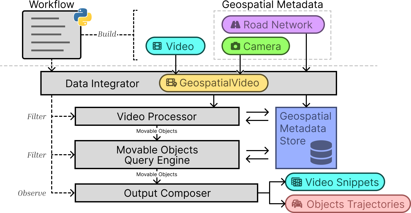
Figure 2. Geospatial Video Analytic Workflow Execution.

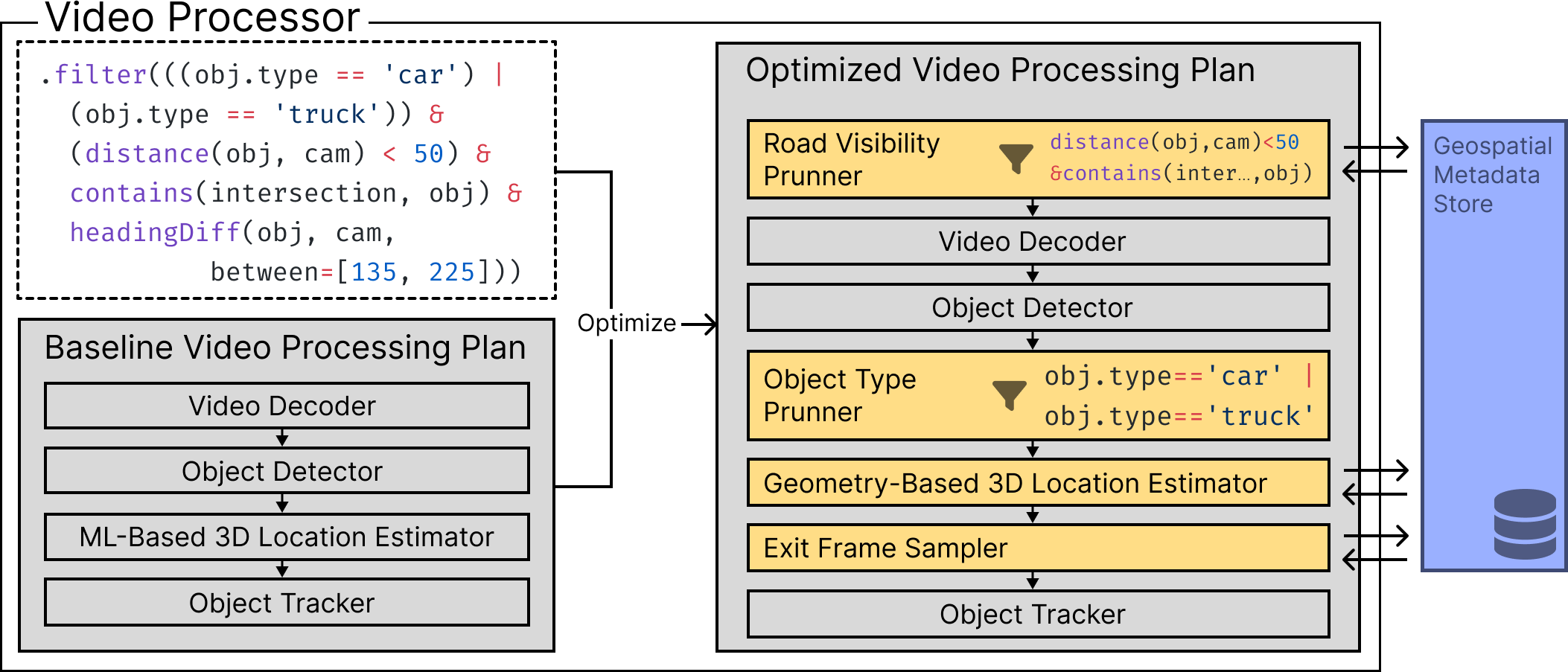
Figure 3. Video Processing Plan for Fig. 1.

6. Video Processing Optimization

We now describe how the video processor executes the workflow. State-of-the-art video inference uses ML models to extract the desired information, such as object positions and their trajectories within each video. Running such models is computationally expensive. Spatialyze’s video processor comes with four optimization techniques to reduce such runtime bottleneck. To be discussed below, the idea behind our optimization is to leverage the geospatial properties of the videos, and the Movable Objects’ inherited physical behaviors. Our optimization techniques include:

• Reducing the number of video frames that needs to be fed into the object detector, object tracker, and 3D location estimator (Sec. 6.1 and Sec. 6.4).

• Reducing the number of objects inputted into the object tracker (Sec. 6.2).

• Replacing a ML-based 3D location estimator with a light-weight function that does not rely on ML at all (Sec. 6.3).

We implement each optimization as a step in the Video Processing stage in Sec. 5.2.2. Besides the existing 4 processing steps in video processor, Spatialyze may place optimization steps in the middle of the video processing plan to reduce the amount of input into later processing steps based on the filter predicates:

• Spatialyze places the Road Visibility Pruner before the decoding step, when users specify the Geographic Constructs the objects of interest must be in. Doing so reduces the number of frames for all other steps in the video processing plan.

• If users filter on object types, then Spatialyze places the Object Type Pruner step right after the Object Detection step. It reduces the number of objects that Spatialyze needs to calculate for their 3D locations and tracking.

• Spatialyze replaces the ML-based 3D Location Estimation step with the much faster 0pt, if Spatialyze can assume that the objects of interest are on the ground, such as cars or people.

• Spatialyze places the Exit Frame Sampler step in between the 3D Location Estimation and the Object Tracking steps, if the users’ predicates focus on cars. It utilizes the 3D locations of the objects and the user-provided metadata to reduce the number of frames that need to be processed by the Object Tracking steps.

Fig. 3 shows where the video processor executes all the optimization steps. Line LABEL:line:pred-contain in Fig. 1 corresponds to Road Visibility Pruner. Line LABEL:line:pred-type filters by object type, so Spatialyze adds Object Type Pruner. The objects of interest are cars or trucks, so Spatialyze adds Exit Frame Sampler and 0pt. In the following sections, we discuss each optimization in detail.

6.1. Road Visibility Pruner

In our experiments, the runtime of ML models (Jocher et al., 2022; Zhou et al., 2019; Du et al., 2023) in the video processing plan takes 90% of the entire workflow execution runtime, on average. Hence, the goal of the Road Visibility Pruner is to remove frames that do not contain objects of user’s interest to reduce the overall runtime of the video processing plan.

6.1.1. High-Level Concepts

The Road Visibility Pruner uses Geographic Construct’s visibility as a proxy for a Movable Object’s visibility. Specifically, if a predicate includes contains(road,obj) and distance(cam,obj) < d; this means that obj is not visible in the frames where road is not visible within d meters; therefore, Spatialyze prunes out those frames. In Fig. 1 for an example, the Road Visibility Pruner partially executes lines LABEL:line:pred-distance-LABEL:line:pred-contain where the user searches for “cars within 50 meters at an intersection.” Using the road’s visibility as proxy, Spatialyze removes all frames that do not contain visible intersection within 50 meters as these frames will not contain any car of users’ interest.

The Road Visibility Pruner only concerns the visibility of Geographic Constructs. Therefore, it uses Geographic Constructs and Camera to decide whether to prune out a video frame. It uses the intrinsic and extrinsic properties of Camera (Zhang, 2014) to determine the viewable area of each of the camera according to the world coordinate system. It then determines if the viewable area of each frame includes any Geographic Construct of interest; frames that do not contain such constructs are dropped and will not be processed in the later stages of the video processing plan. Since the Road Visibility Pruner will be the first step of the video processing plan if applied, it can reduce the number of frames that need to be processed by subsequent ML models in the plan, and hence can substantially reduce overall execution time.

6.1.2. Algorithm

The Road Visibility Pruner works on a per-frame basis. For each video frame $i$ shot by a Camera at location $l_{i}$ with rotation $r_{i}$ and camera intrinsic $it_{i}$, the Road Visibility Pruner performs three steps to determine if the frame should be pruned out. First, it computes the 3D viewable space of the Camera at frame $i$. Then, it uses the viewable space to determine Geographic Constructs that are visible to the Camera at frame $i$. Finally, it uses the users’ filter predicates to determine if there is any Geographic Construct of interest visible in the frame. We explain each step below.

First, the Road Visibility Pruner calculates the 3D viewable space of the Camera at frame $i$. The viewable space is a pyramid (Fig. 4 side view). \small{A}⃝ is the location of the camera. \small{B}⃝, \small{C}⃝, \small{D}⃝, and \small{E}⃝ represent the top-left, top-right, bottom-right, and bottom-left of the frame at $d$ meters in front of the camera. We compute \small{B}⃝, \small{C}⃝, \small{D}⃝, and \small{E}⃝ by converting the mentioned 4 corner points of the frame from pixel coordinates (2D) to world coordinates (3D). This is done in 3 steps by by converting a point from: 1) Pixel to Camera Coordinate System; 2) Camera to World Coordinate System; and 3) Pixel to World Coordinate System.

Pixel Coordinate System to Camera Coordinate System

The equation for converting a 3D point $(x_{c},y_{c},z_{c})$ from camera coordinate system  to a 2D point $(x_{p},y_{p})$ in pixel coordinate system is:

(1) $$\left[\begin{smallmatrix}x_{p}\\ y_{p}\\ 1\end{smallmatrix}\right]=\left[\begin{smallmatrix}f_{x}&s&x_{0}\\ 0&f_{y}&y_{0}\\ 0&0&1\end{smallmatrix}\right]\times\left[\begin{smallmatrix}x_{c}\\ y_{c}\\ z_{c}\end{smallmatrix}\right]\cdot\frac{1}{z_{c}}$$

where $it_{i}=\left[\begin{smallmatrix}f_{x}&s&x_{0}\\ 0&f_{y}&y_{0}\\ 0&0&1\end{smallmatrix}\right]$ is a matrix representing the camera intrinsic, a set of parameters representing Camera’s focal lengths ($f_{x},f_{y}$), skew coefficient ($s$), and optical center in pixels ($x_{0},y_{0}$). The camera intrinsic is a set of parameters specific to each camera, independent of its location and rotation. It is used to convert 3D points from camera perspective to 2D points in pixels.

As our goal is to convert a 2D point in pixel ($x_{p}$ and $y_{p}$), we can find the 3D point in the camera coordinate system ($x_{c}$, $y_{c}$, and $z_{c}$) if we know the distance of the point from the camera ($z_{c}$). From Equation 1, we have:

(2) $$\begin{split}\left[\begin{smallmatrix}x_{c}\\ y_{c}\\ z_{c}\end{smallmatrix}\right]&=\left[\begin{smallmatrix}f_{x}&s&x_{0}\\ 0&f_{y}&y_{0}\\ 0&0&1\end{smallmatrix}\right]^{-1}\times\left[\begin{smallmatrix}x_{p}\\ y_{p}\\ 1\end{smallmatrix}\right]\cdot z_{c}\\ &=\left[\begin{smallmatrix}1/f_{x}&-s/(f_{x}f_{y})&(sy_{0}-f_{y}x_{0})/(f_{x}f_{y})\\ 0&1/f_{y}&-y_{0}/f_{y}\\ 0&0&1\end{smallmatrix}\right]\times\left[\begin{smallmatrix}x_{p}\\ y_{p}\\ 1\end{smallmatrix}\right]\cdot z_{c}\end{split}$$

Modifying Equation 2 so that the left side is $[x_{c},y_{c},z_{c},1]^{\top}$,

(3) $$\begin{split}\left[\begin{smallmatrix}x_{c}\\ y_{c}\\ z_{c}\\ 1\end{smallmatrix}\right]&=\left[\begin{smallmatrix}1/f_{x}&-s/(f_{x}f_{y})&(sy_{0}-f_{y}x_{0})/(f_{x}f_{y})&0\\ 0&1/f_{y}&-y_{0}/f_{y}&0\\ 0&0&1&0\\ 0&0&0&1\end{smallmatrix}\right]\times\left[\begin{smallmatrix}x_{p}z_{c}\\ y_{p}z_{c}\\ z_{c}\\ 1\end{smallmatrix}\right]\\ &=C\times\left[\begin{smallmatrix}x_{p}z_{c}&y_{p}z_{c}&z_{c}&1\end{smallmatrix}\right]^{\top}\\ \end{split}$$

where $C=\left[\begin{smallmatrix}1/f_{x}&-s/(f_{x}f_{y})&(sy_{0}-f_{y}x_{0})/(f_{x}f_{y})&0\\ 0&1/f_{y}&-y_{0}/f_{y}&0\\ 0&0&1&0\\ 0&0&0&1\end{smallmatrix}\right]$

Camera Coordinate System to World Coordinate System

For this conversion, we set up $R$, a $3\times 3$ matrix, representing the 3D rotation of the camera that is derived from the camera’s rotation quaternion. And $t$ is a 3D vector that represents the camera’s translation. Then, $[R|t]$ is a $3\times 4$ extrinsic matrix for converting 3D points from camera coordinate system $(x_{c},y_{c},z_{c})$ to 3D points $(x,y,z)$ in world coordinate system (Zhang, 2014):

(4) $$\left[\begin{smallmatrix}x&y&z\end{smallmatrix}\right]^{\top}=[R|t]\times\left[\begin{smallmatrix}x_{c}&y_{c}&z_{c}&1\end{smallmatrix}\right]^{\top}$$

Pixel Coordiante System to World Coordinate System

Combining the previous 2 conversions in Equation 3 and Equation 4, we can now convert 2D points from pixel-coordinate system to 3D points from world coordinate system using:

(5) $$\begin{split}\left[\begin{smallmatrix}x&y&z\end{smallmatrix}\right]^{\top}&=[R|t]\times C\times\left[\begin{smallmatrix}x_{p}z_{c}&y_{p}z_{c}&z_{c}&1\end{smallmatrix}\right]^{\top}\end{split}$$

4 corners of a video frame in World Coordinate System

To convert the 4 corners of a video frame from pixel to world coordinates, we modify Equation 5 where we substitute $z_{c}$ with $d$, and $x_{p}$ and $y_{p}$ with actual pixel values representing the 4 corners of the video frame; $w$ and $h$ are the width and height in pixels of the video frame, and each of $B,C,D,E$ is a $3\times 1$ vector representing its 3D location.

(6) $$\left[\begin{smallmatrix}B&C&D&E\end{smallmatrix}\right]=[R|t]\times C\times\left[\begin{smallmatrix}0&wd&wd&0\\ 0&0&hd&hd\\ d&d&d&d\\ 1&1&1&1\end{smallmatrix}\right]$$

After the corners of each frame are translated to world coordinates, the Road Visibility Pruner uses the viewable space to determine the Geographic Constructs that are visible by Camera at frame $i$. Each Geographic Construct’s area is defined using a 2D polygon. Specifically, all polygons representing Geographic Constructs are 2D in the $z=0$ plane. Therefore, the Road Visibility Pruner projects the computed 3D viewable space onto the $z=0$ plane. We define the top-down 2D viewable area as the convex hull (Sklansky, 1982) of the projected vertices \small{A}⃝, \small{B}⃝, \small{C}⃝, \small{D}⃝, and \small{E}⃝ (yellow highlight in Fig. 4’s top view). Any Geometric Construct that overlaps with the 2D viewable area is considered visible to the Camera at frame $i$. Once computed, we get visibleGTypes, a set of Geometric Construct types that are visible to the Camera at frame $i$.

Finally, the Road Visibility Pruner uses the users’ filter predicates to determine if there is any Geographic Construct of interest visible in the frame. It starts by examining the contains predicates in the filter. Then, it assigns each contains to $True$ if its first argument’s type is in visibleGTypes and $False$ otherwise. If the value of the transformed filter predicates is $False$, then the Road Visibility Pruner prunes out that frame.

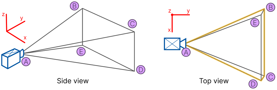
Figure 4. (Side) A 3D viewable space of a camera in pyramid shaped. (Top) Projected area of the pyramid onto $z=0$ plane.

6.1.3. Benefits and Limitations

The Road Visibility Pruner has an insignificant overhead runtime compared to the runtime it can save. Our experiments show that the Road Visibility Pruner takes 0.1% of the video processing runtime to execute, while saving up to 19.6% of the video processing runtime. So in the worst case that Road Visibility Pruner cannot prune out any video frames, the runtime increase is still negligible. However, having the Road Visibility Pruner in the video processing plan may cause tracking accuracy to drop in some scenarios. Using Sec. 3 as an example, if a car starts at an intersection, exits the intersection, and enters an intersection again. During the time that the car is not in any intersection, the camera may not capture any frames containing intersection. The Road Visibility Pruner will prune out the period of video frames where there is no intersection visible to the camera. This can lead to the object tracking algorithm considering the car before leaving the intersection and the car after entering the intersection for the second time to be two different cars.

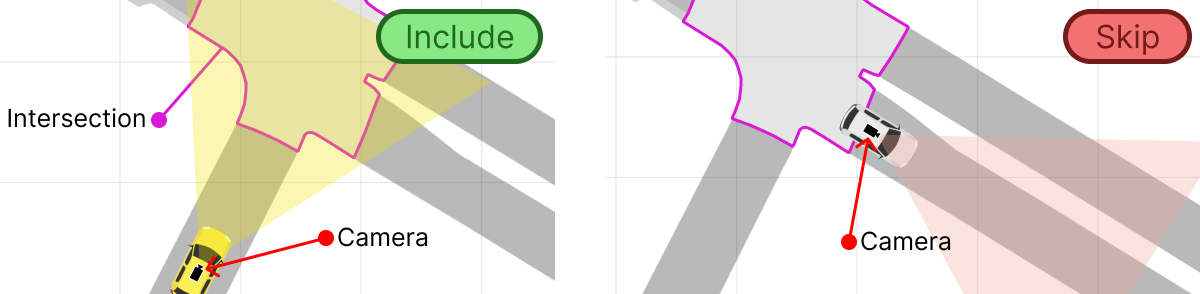
Figure 5. Sec. 3’s workflow looks for a car on an intersection; therefore, the video processor executes expensive ML models only on video frames with a visible intersection.

6.2. Object Type Pruner

The SORT-Family (Du et al., 2023; Wojke et al., 2017; Bewley et al., 2016) algorithms use the Hungarian method (Kuhn, 1955) to associate objects between each 2 consecutive video frames. The runtime of the Hungarian method scales with the number of objects to associate in each frame. Reducing the number of objects input into SORT-Family algorithms can hence directly reduce the runtime of the object tracking step of the plan.

6.2.1. High-Level Concepts

Spatialyze only needs to track objects that are of interest as stated in the workflow. The emphObject Type Pruner prunes out irrelevant objects from being tracked. We analyze users’ filter predicates to look for types of objects that are necessary for computing the workflow outputs. Using the predicates in Fig. 1 as an example, the Object Type Pruner partially executes the line LABEL:line:pred-type, where users only look for cars and trucks in the workflow outputs. The trajectories of other objects (e.g., humans or traffic lights) will not appear in the final workflow outputs anyway, so tracking them is unnecessary. Therefore, we only need to input objects that are detected as cars or trucks into object tracker to reduce its workload.

6.2.2. Benefits and Limitations

The Object Type Pruner primarily reduces object tracker’s runtime. Nevertheless, the Object Type Pruner has low overhead runtime of 0.06% and does not require any geospatial metadata, but can reduce up to 69% of the runtime spent on object tracking, which is 26% of the video processor runtime.

6.3. 0pt

Spatialyze uses an object’s distance from camera and its calculated bounding box to estimate its 3D location in our video processing plan. Specifically, we use YOLOv5 (Jocher et al., 2022) to estimate the bounding box and Monocular Depth Estimator (Godard et al., 2019) (Monodepth2) to estimate the object’s distance from camera in our baseline plan. Monodepth2 only requires monocular images (videos) to estimate each object’s distance from camera; therefore, it is extremely flexible in general use cases. Spatialyze can always use Monodepth2 to estimate any object’s distance from camera in a video frame. However, this algorithm is slow and can take upto 48% portion of the total baseline video processing runtime. Therefore, we explored an alternative algorithm that leverage existing geospatial metadata to speed up the process for estimating 3D object location.

6.3.1. High-Level Concepts

0pt leverages Camera to estimate an object’s 3D locations from its 2D bounding box. It is a substitution for Monodepth2 to estimate objects’ 3D locations. 0pt uses basic geometry calculations and requires 2 assumptions to hold. First, the object of interest must be on the ground. We can then assume that the lower horizontal border of the object’s bounding box is the point where the object touches the ground. Second, we can identify the equation of the plane that the object of interest is on. In Spatialyze, the plane $z=0$ is the ground, although our algorithm can be modified to use with any plane. The middle point of the lower border of each object’s 2D bounding box represents the point that it touches the ground (red star in Fig. 6).

6.3.2. Algorithm

0pt performs 2 steps to estimate 3D location of an object from its 2D bounding box. First, based on the second assumption, 0pt finds an equation that represents a Vector of Possible 3D Locations of an object. Second, based on the first and third assumptions, 0pt finds an Exact 3D Location from the vector that intersects with the ground.

Vector of Possible 3D Locations

Using Equation 5, we convert any 2D point in pixel coordinate system to a 3D point in world coordinate system, if we know $z_{c}$. Since we do not know $z_{c}$ in this case, we can derive a parametric equation representing all possible 3D points (red line in Fig. 6) converted from the 2D point. Let $d$ be the unknown distance of the object from the camera.

(7) $$\begin{split}\begin{bmatrix}x&y&z\end{bmatrix}^{\top}&=[R|t]\times C\times\begin{bmatrix}x_{p}d&y_{p}d&d&1\end{bmatrix}^{\top}\end{split}$$

Exact 3D Location

From our assumptions, we know that the bottom line of the object’s bounding box touches the ground. Therefore, $(x,y,z)$ also touches the ground. Because the ground is $z=0$ in our case, we can solve the Equation 7 for $d$. Once we know $d$, we can solve the parametric Equation 7 for $x$ and $y$ (blue star in Fig. 6).

6.3.3. Benefits and Limitations

0pt relies on the assumptions mentioned, which do not always hold, especially, the first one. Nevertheless, Spatialyze can analyze users’ filter predicates and tell whether the types of objects of interest can be assumed to touch the ground and only applies the optimization then. For example, “car,” “bicycle,” or “human” touch the ground, while “traffic light” does not. In addition, 0pt is 192$\times$ faster compared than Monodepth2 on average. If one of the estimated 3D locations of an object in a video frame ends up being behind the camera, which means that the object does not touch the ground, Spatialyze can fall back to use Monodepth2 for that frame. Otherwise, 0pt provides 99.48% runtime reduction on average for object 3D location estimation and 52% for the video processing.

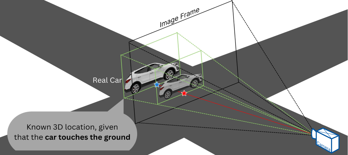
Figure 6. 0pt recovers the 3D location (blue star) of a car from its 2D location (red star).

6.4. Exit Frame Sampler

Object trajectories are computed in the object tracker step (Sec. 5.2.2) using an object tracking algorithm. Such algorithms, including that used in Spatialyze, perform tracking-by-detection (Leal-Taixé, 2014). An object detector detects objects in each video frame, but it does not determine which detections across multiple frames represent the same object. The object tracker performs data association by going through each frame and associating detections in the current frame to detections in the latest frame it previously performed data association on. As a result, a chain of associated detections represents an object trajectory, in this case, a Movable Object. However, not all detections are necessary in an object trajectory. For instance, suppose a car travels in a straight line from frame 1 to frame 3, where it is at location (0, 1) at frame 1, (0, 2) at frame 2, and (0, 3) at frame 3. The in-between detection (0, 2) at frame 2 is unnecessary as the detections at frame 1 and frame 3 produce the same straight-line trajectory.

Spatialyze’s Exit Frame Sampler utilizes users’ geospatial metadata (Camera and RoadNetwork) to heuristically prune out video frames that are likely to contain such unnecessary detections, by sampling only the frames that may contain at least one necessary detection. As a result, the object tracker only needs to perform data association on fewer frames, significantly reducing its runtime.

6.4.1. High-Level Concepts

Suppose a car is visible to a Camera and driving in a lane. As discussed in Sec. 4.1.1, a Movable Object of type “car” has 2 inherited physical behaviors: it follows the lane’s direction and travels at the speed limit regulated by traffic rules. The Exit Frame Sampler leverages these behaviors to estimate the trajectory of the car so that the object tracker need not perform data association on any frame from now on before any of the following events happens: i) a car exits its current lane; ii) a car exits the Camera’s view; iii) a new car enters the Camera’s view. These events are sampleEvents. The Exit Frame Sampler samples the frame when a sampleEvent happens for the object tracker to perform data association. The followings are the reasons.

For (i), when the car is in a lane, without object tracking, the Exit Frame Sampler assumes that it follows the lane’s direction until it reaches the end of the lane. After it exits the lane, it may enter an intersection and stop traveling in a straight line. To maintain the accuracy of the trajectory, the object tracker needs to perform data association at the frame right before the car exits the lane. In contrast, if the car is already at an intersection, it may not travel in a straight line; therefore, the object tracker cannot skip any frame.

Event (ii) is the first frame that the car is no longer visible to the Camera. If this event happens before the car exits its lane, although the car’s trajectory still continues in the lane, the object tracker needs to perform data association at the frame before the car is no longer visible to the Camera as the end of the car’s trajectory.

For (iii), if a new car enters the camera’s view, the object tracker needs to start tracking the new car at that frame.

If a frame contains multiple cars, the Exit Frame Sampler skips to the earliest frame that (i), (ii), or (iii) is estimated to happen for any car, which prevents incorrect tracking for any of them. We implement this idea as our sampling algorithm where given a current frame and its detected cars, it samples the next frame for the object tracker to perform data association. The Exit Frame Sampler executes this algorithm starting from the first frame of a video to find the next frame and skips to it. Then it repeats the procedure until the end of the video. In the end, the Exit Frame Sampler passes a list of frame numbers to the object tracker step to perform data association on.

Because the algorithm depends on the 2 mentioned inherited physical behaviors, it only works when users filter for Movable Objects with such behaviors, such as vehicles. Therefore, the video processor only adds the Exit Frame Sampler when users’ workflow Filters on the object type being vehicles.

6.4.2. Sampling Algorithm

Fig. 7 shows how the Exit Frame Sampler implements each sampleEvent mentioned above.

exitsLane implements (i) when the car exits the lane. Given the car’s location at the current frame (carLoc) and the lane that contains the car, we assume that the car drives in the lane straight along the lane’s direction. In line LABEL:line:exit-lane-loc, we model the car’s movement as a motion tuple (carLoc, lane.direction). We compute the intersection between the car’s motion tuple and the lane as the location where the car exits the lane. Given the car’s moving speed v, we know the time it reaches the exit location starting from the time of the current frame in line LABEL:line:exit-lane-time. We sample the last frame before the car reaches the exit location.

exitsCamera implements (ii) when the car exits the camera’s view. Knowing the car’s current location, moving direction, and speed, carMoves computes its location at any given frame after the current frame in line LABEL:line:car-moves. Then in line LABEL:line:view-contain, we use the viewable area of the Camera at each frame derived from Sec. 6.1 to find the first frame when the car’s location is not in the camera’s view of that frame. This is the frame when the car already exits the camera’s view, so we sample the frame before it.

newCar implements (iii) when a new car enters the Camera’s view. In line LABEL:line:more-car, we sample the first frame after the current one with more cars. The number of cars is a good heuristic to predict new arrivals because if this is the sampleEvent we choose eventually, it means that this event happens first—none of the cars have exited the camera’s view yet. So, the total number of cars has not changed if there is no new car entering the frame.

With the implementation of the sampleEvents, at the current frame, the Exit Frame Sampler first finds the frame in which we have more detections for sampleEvent (iii). Then for each car, the Exit Frame Sampler computes the frames to sample for sampleEvents (i) and (ii). Among (i), (ii), (iii), the Exit Frame Sampler choose the earliest sampleEvent as the next frame for the object tracker to perform data associations.

⬇

def exitsLane(currentFrame, carLoc, lane, v, cameras):

exitLaneLoc = intersection((carLoc, lane.direction), lane)!$\label{line:exit-lane-loc}$!

exitLaneTime = cameras[currentFrame].time +

distance(exitLaneLoc, carLoc) / v!$\label{line:exit-lane-time}$!

return lastFrameBefore(exitLaneTime) !$\label{line:last-frame}$!

def exitsCamera(currentFrame, carLoc, lane, v, cameras):

nextFrame = currentFrame + 1

while cameras[nextFrame].view.contains(!$\label{line:view-contain}$!

carMoves(carLoc, lane.direction, v, !$\label{line:car-moves}$!

cameras[nextFrame].time - cameras[currentFrame].time)):

nextFrame += 1

return lastFrameBefore(nextFrame)

def newCar(currentFrame):

nextFrame = currentFrame + 1

while numCars(nextFrame) <= numCars(currentFrame):!$\label{line:more-car}$!

nextFrame += 1

return nextFrame

Figure 7. Computing the events that might trigger a frame sample

6.4.3. Sampling Algorithm Walk-through

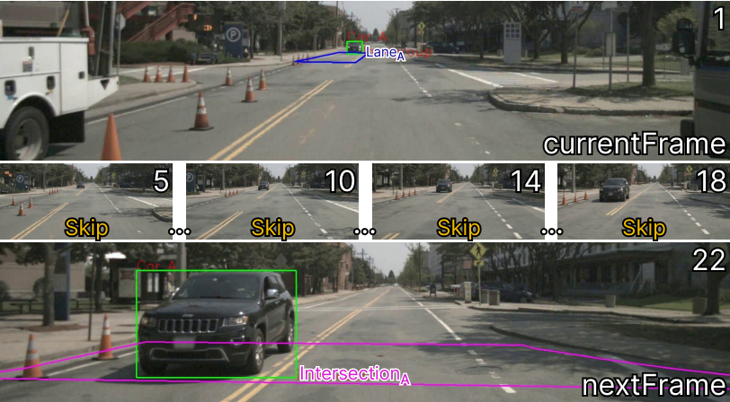
Figure 8. Example Results of Sampling Algorithm

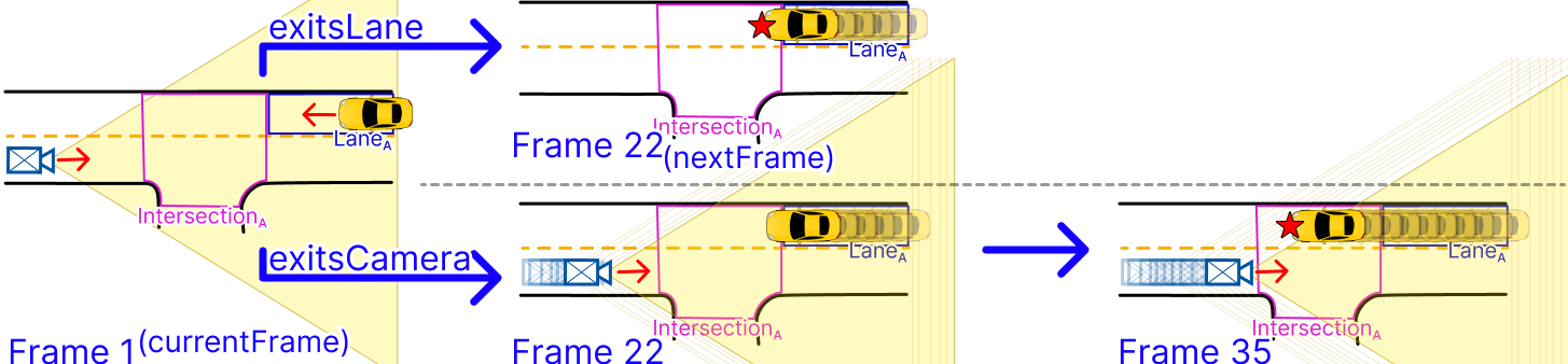
Figure 9. Sample Events exitsLane (i) and exitsCamera (ii)

Frame number 1 labeled as currentFrame in Fig. 8 was taken at 3:51:49.5 PM. Now, we illustrate how the Exit Frame Sampler gets the next frame to sample. In this frame, our object detector only detects one car, $Car_{A}$. The 3D Location Estimator step calculates its 3D location to be (70.92, 74.7, 0). We know the direction of $Lane_{A}$ is 181° counterclockwise from the east. We assume the car’s speed is 25mph based on common traffic rules. We also have the viewable area of all frames.

First, we compute the sampleEvent when there are new cars entering $Camera_{B}$’s view through newCar(currentFrame=1). We find that for the rest of the videos, there is only one car in the frame.

Then, we compute the sampleEvent when $Car_{A}$ exits $Lane_{A}$ through exitsLane(currentFrame=1,carLoc=(70.92, 74.7, 0), lane=$Lane_{A}$,v=25mph,$cameras$). In line LABEL:line:exit-lane-loc, $Car_{A}$’s motion tuple intersects $Lane_{A}$ at location (66.3, 72.7, 0) and $Car_{A}$ is estimated to reach there at 3:51:49.96 PM in line LABEL:line:exit-lane-time. We then find that the last frame before this time is frame 22, depicted as exitsLane in Fig. 9.

Finally, we compute the sampleEvent when $Car_{A}$ exits the $Camera_{B}$’s view through exitsCamera(currentFrame=1, carLoc=(70.92, 74.7, 0), lane=$Lane_{A}$, v=25mph, $cameras$). We find that the camera view of frame 35 does not contain $Car_{A}$’s position at frame 35 computed in line LABEL:line:car-moves. Therefore, we return frame 34 to sample, depicted as exitsCamera in Fig. 9.

Among the three sampleEvents, exitsLane in Fig. 9 returns frame 22, which is the earliest. Thus, the Exit Frame Sampler samples the last frame before $Car_{A}$ exits its lane at frame 22 labeled as nextFrame in Fig. 8, skipping all frames in between labeled “Skip.” The Exit Frame Sampler then repeats the algorithm to sample frames until it reaches the end of the video.

6.4.4. Benefits and Limitations

To show the effectiveness of the Exit Frame Sampler. we define the skipping ratio as $\scriptstyle\frac{\text{\# of frames skipped}}{\text{total \# of frames}}$. We benchmarked the average runtime of the object tracker when hardcoding the Exit Frame Sampler to report different skipping ratios. It decreases linearly as the Exit Frame Sampler skips more frames. When the skipping ratio is 30%, the average tracking runtime decreases by almost 50%. The real skipping ratio by the Exit Frame Sampler depends on the assumption of the maximum car speed. For common traffic conditions, the speed limit is 25 mph on lanes; the average skipping ratio on our experimental dataset is 13.1% which gives us 9.1% speed up in running our tracker.

Admittedly, the sampling algorithm may over-skip and the object tracker may lose track of the cars of interest. To diagnose if the Exit Frame Sampler suffers from this risk, we derived a maximum skipping threshold. We sample a set of videos. For each object in each video, we exhaustively search for the maximum skipping size before our tracker loses track of the object. Then, we take the median of all maximum skipping sizes from these tracks as the skipping threshold which is 5. We then constraint the Exit Frame Sampler to not skip more than 5 frames and got a +1% accuracy increase. This adds to the confidence in our implementation against over-skipping.

7. Evaluation

We have implemented a prototype of Spatialyze and evaluated its different components of against other state-of-the-art techniques. We also evaluate our optimization techniques with an ablation study by comparing Spatialyze’s video processing plans with and without each of them.

7.1. Experiments Setup

Queries

We implemented Spatialyze’s workflows using four realistic road scenarios, inspired by scenarios from Kim et al. (Kim et al., 2021b). These workflows allowed us to test Spatialyze against real-life situations, with varying conditions for each of them. The workflow started form loading in RoadNetworks and 240 Videos with their Cameras, similar to lines LABEL:line:world-LABEL:line:end-build in Fig. 1. Then, we filter the videos with one of the queries described below, similar to lines LABEL:line:object-LABEL:line:pred-heading. All queries look for nearby objects (closer than 50 meters). Finally, we save the filtered videos into video snippets files, similar to line LABEL:line:observe. Below are descriptions of the queries in natural language, as each of the systems that we compare against have their own syntax:

1. A pedestrian at an intersection facing perpendicularly to that of a camera mounted on a car.

2. 2 cars at an intersection moving in opposite directions.

3. Camera moving in the direction opposite to the lane direction, with another car (which is moving in the direction of the lane) within 10 meters of it.

4. A car and a camera moving together in the same direction on lanes; 2 other cars moving together on opposite lanes.

Dataset

We use the multi-modal AV datasets used in Kim et al. to evaluate Spatialyze. They comprise of 3 datasets that are needed for executing the 4 queries mentioned: 1) videos from on-vehicle cameras, 2) the cameras’ movement and specification, and 3) road network of Boston Seaport where the videos were shot. The former 2 datasets are directly from nuScenes (Caesar et al., 2019) (training set), and the later is from Scenic (Kim et al., 2021b; Fremont et al., 2020, 2019). From nuScenes, we randomly sampled 80 out of 467 scenes that are captured at the Boston Seaport from on-vehicle cameras; we chose videos from 3 front cameras for each scene; each video is 20 seconds long at 12 Hz. The runtime of Spatialyze’s execution per video does not depend on the number of input video; therefore, we have determined that 240 sampled videos are sufficient to demonstrate our contributions in Spatialyze.

Hardware

To run our experiments, we use Google Cloud Compute Engine with Nvidia T4; n1-highmem-4 Machine with 2 vCPUs (2 cores), 26 GB of Memory; and Balanced persistent disk.

7.2. Comparison with Other Systems

7.2.1. EVA

We compare the run-time of the Spatialyze pipeline with that of our EVA (Xu et al., 2022) implementation using the same queries. EVA is a VDBMS that allows for the definition of custom user-defined functions (UDFs), and also preforms a number of optimizations. Since EVA executes the queries on a frame-by-frame basis, it cannot compute object tracks (and hence object directions), so we modified the queries in our test to query for frames where:

1. A pedestrian is at an intersection.

2. 2 cars are at an intersection.

3. A car is on a lane within 10 meters of the camera.

4. 3 cars, each on a lane.

To make use of EVA ’s caching mechanisms, we compare with the run-times of the queries when they are run in series without resetting EVA and its database (so running QE1 directly after QE2, QE3 directly after QE2, and so on). The results are presented in Table 1.

Query	Spatialyze		EVA
	Runtime	LoC	Runtime	LoC
QE1	3.0 sec.	14	138.0 sec.	60
QE2	3.4 sec.	19	235.9 sec.	61
QE3	6.2 sec.	16	127.8 sec.	60
QE4	33.4 sec.	30	236.2 sec.	58
Shared		0		286

Table 1. Comparison of Spatialyze to EVA in terms of runtime-per-video and LoCs (lines of code). Shared lines are LoC that are used for both queries, e.g., object detection UDFs.

As shown, Spatialyze performs 7-68$\times$ faster with respect to EVA on these four queries. This is mainly because of Spatialyze not needing to run Monodepth depth detection on each frame, due to the Object Type Pruner and 0pt optimizations. In addition, Spatialyze shaves even more time by employing the Road Visibility Pruner to avoid costly YOLO and depth detections on frames where they are unnecessary. We also compare the line counts between the different systems and present these results in Table 1, where it is clear Spatialyze also makes query implementation much easier and requires less lines of code (LoC) to achieve the same result.

7.2.2. nuScenes

We compare the run-time of the Movable Objects Query Engine stage with the same queries implemented using the nuScenes Devkit (Caesar et al., 2019). NuScenes Devkit is a Python API used to query results from the nuScenes dataset (Caesar et al., 2019). We only compare the Movable Objects Query Engine stage as Devkit operates on already processed videos and ingested object annotations. Table 2 contains the results of this comparison.

Query	Spatialyze		nuScenes Devkit
	Runtime	LoC	Runtime	LoC
Q1	0.013 sec.	12	4.747 sec.	55
Q2	0.055 sec	18	39.390 sec.	61
Q3	0.114 sec.	14	13.348 sec.	66
Q4	1.551 sec.	29	Timed Out	123
Shared		0		78

Table 2. Comparison of Spatialyze to nuScenes Devkit in terms of runtime-per-video and LoCs (lines of code). Shared LoCs are LoCs that are used for all four queries.

As seen in Table 2, the Devkit implementation of Q4 (the query that dealt with 3 objects) timed out before finishing and producing a result; it ran out of memory during execution due to the creation of too many Python objects, as a result of materializing all possible combinations of 3 object tuples in memory before filtering them. It also takes significantly longer on average to execute the same query as Spatialyze, with Spatialyze achieving a 117-716$\times$ faster runtime. Two of the main factors that allow Spatialyze to achieve this better execution time are the following. First, Spatialyze pre-processes the road network data, generating additional columns and indexes that allow it to avoid costly joins, which contribute greatly to the large execution time of Devkit. Second, certain Devkit functions perform costly linear algebra that are avoided by Spatialyze using the geospatial metadata store. One example is when checking if an object is in the view of a camera. Devkit does this by projecting the 3D location onto the 2D frame, while Spatialyze uses the pre-stored view angle of the camera to quickly identify if the object is contained inside the camera frame or not. We once again compare the line count between the different systems, and present these results in Table 2, where we can see that the Spatialyze implementation once again takes far less lines of code.

7.2.3. OTIF

OTIF (Bastani and Madden, 2022) is a general-purpose object tracking algorithm that trains a segmentation proxy model and a recurrent method to reduce the frame sampling rate that is needed to get object tracks in the video. We compare the run-time of the Video Processor of Spatialyze with that of OTIF on computing tracks. We run each of the two systems on 240 randomly selected videos of our experiment dataset, and compare the average runtime per video. The training time of OTIF is 61m37s. After it is trained when the query asks for tracks of a certain object type such as cars or pedestrians, OTIF needs to spend 13.47s per video getting all the classified tracks before it can filter on object types. Since OTIF is not aware of the Geographic Constructs, if the query further filters objects on a specific RoadNetwork such as an intersection, in addition to the 13.47s tracking time, OTIF needs to do extra work to get the 3D coordinates of the tracks and filter them on the RoadNetworks. But for Spatialyze, our video processor applies all optimizations elaborated in Sec. 6, and it only takes 9.6s to get the tracks for each video. In fact, the runtime of Spatialyze to compute tracks is less than OTIF even without counting OTIF’s training time.

7.3. Ablation Study

To evaluate each of our optimization techniques, we manually construct video processing plans for the following 7 experiment setups. (SB) Baseline is a Baseline plan without any optimization. It includes the 4 processing steps mentioned discussed in Sec. 5.2.2. (S1) is the Baseline plan with the Road Visibility Pruner. (S2) is the Baseline plan with the Object Type Pruner. (S3) is the Baseline plan with Monocular Depth Estimator replaced with the 0pt. (S4) is the Baseline plan with the Exit Frame Sampler. (S5) is a plan with all optimizations except the Exit Frame Sampler. (S6) is a plan with all optimizations.

7.3.1. Execution time

The average runtime of our workflow execution without any optimization is 34 seconds for each video. When broken down, 0.01% of the time is spent in the Data Integrator; 89.9% in Video Processor; 9.5% in Movable Objects Query Engine; 0.6% in Output Composer. In this section, we evaluate the effect of each of our optimization techniques, by executing Spatialyze on the workflows discussed in Sec. 7.1. Because the video processing plans for Q3 and Q4 are the same, we do not discuss Q4 in this section.

Applying all optimization techniques, we achieve 2.5-5.3$\times$ speed up over the baseline plan, as shown in Fig. 10. The Road Visibility Pruner reduces the runtime of the entire plan. In Q3, it prunes out the frames that do not contain “lane,” which is 3.8% of the total amount. In Q1-2, the Road Visibility Pruner prunes out frames that do not contain “intersection.” “Intersections” are less common than “lanes” on the street, so the Road Visibility Pruner prunes out more frames at 21.5% of the total amount, resulting in 20.0% runtime reduction. The Object Type Pruner only reduces the runtime of StrongSORT. For Q2-4, the Object Type Pruner prunes out objects that are not cars or trucks, which is 36.5% of all objects, resulting in 7.0% runtime reduction. For Q1, the Object Type Pruner prunes out objects that are not pedestrians. The Object Type Pruner is more effective in this scenario as pedestrians are less frequent on the street. It prunes out 86.3% of all objects, resulting in 26.3% runtime reduction. The 0pt makes the runtime portion of 3D location estimation insignificant (from 48% to 0.55%). Q1 does not execute the Exit Frame Sampler because it only works with cars or trucks. The Exit Frame Sampler has an overhead runtime of executing Sec. 6.4.2; however, it significantly reduce the number of frames into StrongSORT (13.1%), resulting in 0.8% runtime reduction.

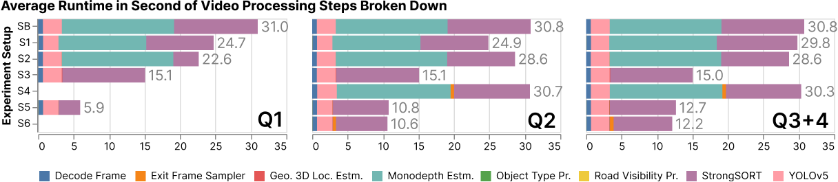
Figure 10. Average video processing time for each video of 20 seconds, comparing each optimization technique.

7.3.2. Accuracy

Our optimization techniques can potentially reduce object tracking accuracy as a result of dropping frames. To quantify this, we evaluate our optimization techniques using the execution results from (SB) setup as the ground truth. Then, we compare the the execution results from other setups against that of the (SB). We evaluate the accuracy for our two observer functions. First, because getObjects outputs Movable Objects and their tracks, we measure how each of our optimization techniques affects the tracking accuracy of the video processor. Second, because saveVideos saves snippets of videos that matches users’ query predicates, we measure how each of our optimization techniques affects the accuracy of the saved videos.

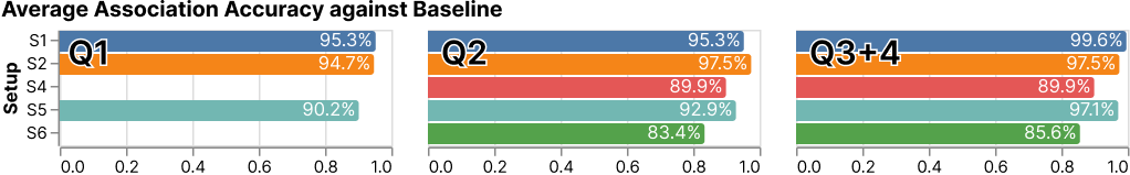
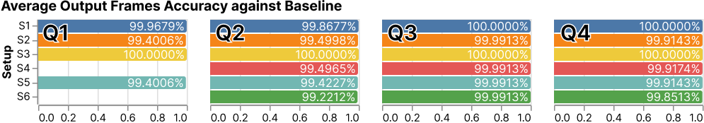
Figure 11. Association and video frames output accuracy against Baseline compared between experiment setups.

Tracking Output Accuracy

We evaluate our tracking accuracy of each experiment setup by comparing the tracking output from the experiment setup with the tracking output from (SB) setup, using HOTA (Luiten et al., 2020), an evaluation metric for measuring multi-object tracking accuracy. Using the ground truth trackings from a video and prediction trackings from the same video, HOTA returns an Association Accuracy (AssA), ranging from 0 to 1. AssA of 0 means that the prediction trackings are completely incorrect, and 1 means that the prediction trackings are the same as the ground truth. In this evaluation, the ground truth trackings are the tracking results from the (SB) setup, and the prediction trackings are the tracking results from each of the other setups. In Q1, we only compare the association accuracy of persons because Q1 does not produce any other object type. Similarly, in Q2-Q4, we only compare the association accuracy of cars and trucks. We also exclude object detections from the frame pruned by the Road Visibility Pruner because this pruning is a part of users’ predicates and will not be output for the users.

In Fig. 11, the Road Visibility Pruner (S1) causes a small accuracy drop of 0.4% for Q3-4 and 4.7% for Q1-2. The Object Type Pruner (S2) also causes a small accuracy drop of 2.5% from Q2-4 and 5.3% for Q1. We do not include 0pt (S3) into the results; since the object tracker only concerns the 2D bounding boxes of objects, 0pt does not affect the accuracy of the object tracker. Combining all 3 optimization techniques (S5), the video processor still produces accurate object tracks of 93.4% on average compared to (SB), while speeding up 2.5-5.3$\times$ of its runtime. With all optimization techniques (S6), the video processor’s accuracy for object tracking is 15.5% on average, while speeding up 1.65-4.32%, additionally.

Video Frame Output Accuracy

To compare the accuracy of video frames output, we execute Q1-4 with Spatialyze and compare the video frames output from each experiment setup with the video frames output from (SB). For each video in a setup, the video frame accuracy is the number of frames the plan outputs or drops correctly divided by the total number of frames. For example, for a video with 4 frames, if (SB) outputs frame 2 while plan X outputs frame 2 and 3, then the accuracy score for plan X is $3/4$ because plan X correctly outputs 2 and correctly dismisses frames 1 and 4.

Our results in Fig. 11 show that all of our optimization techniques have low negative impact to the accuracy of video processor. Specifically, Spatialyze can still accurately output and dismiss video frames with all of our optimization techniques. Notably, our 0pt does not have any negative impact on Spatialyze’s frame output accuracy on our evaluation datasets and experiment set up at all. These results show the accuracy of the 0pt in estimating objects 3D locations. The accuracy is comparable to that of the baseline ML-based approach that uses Monodepth2 (Godard et al., 2019) while providing 192$\times$ runtime speedup on average, causing 51.75% runtime reduction of the video processor on average.

8. Conclusion

We presented Spatialyze, a system for geospatial video analytics that leverages existing geospatial metadata and inherited physical behavior of objects in videos to speed up video processing. Spatialyze’s DSL, S-FLow, allows users to declaratively specify their geospatial video workflows using our build-filter-observe paradigm, and our evaluations show Spatialyze’s efficiency in processing geospatial video workflows when compared to state-of-the-art tools.

References

- (1)
- Anwar (2022) Aqeel Anwar. 2022. What are Intrinsic and Extrinsic Camera Parameters in Computer Vision? https://towardsdatascience.com/what-are-intrinsic-and-extrinsic-camera-parameters-in-computer-vision-7071b72fb8ec. Accessed: 2023-07-25.
- Bastani et al. (2020) Favyen Bastani, Songtao He, Arjun Balasingam, Karthik Gopalakrishnan, Mohammad Alizadeh, Hari Balakrishnan, Michael Cafarella, Tim Kraska, and Sam Madden. 2020. MIRIS: Fast Object Track Queries in Video. In Proceedings of the 2020 ACM SIGMOD International Conference on Management of Data (Portland, OR, USA) (SIGMOD ’20). Association for Computing Machinery, New York, NY, USA, 1907–1921. https://doi.org/10.1145/3318464.3389692
- Bastani and Madden (2022) Favyen Bastani and Samuel Madden. 2022. OTIF: Efficient Tracker Pre-Processing over Large Video Datasets. In Proceedings of the 2022 International Conference on Management of Data (Philadelphia, PA, USA) (SIGMOD ’22). Association for Computing Machinery, New York, NY, USA, 2091–2104. https://doi.org/10.1145/3514221.3517835
- Bewley et al. (2016) Alex Bewley, Zongyuan Ge, Lionel Ott, Fabio Ramos, and Ben Upcroft. 2016. Simple online and realtime tracking. In 2016 IEEE International Conference on Image Processing (ICIP). IEEE. https://doi.org/10.1109/icip.2016.7533003
- Bradski (2000) G. Bradski. 2000. The OpenCV Library. Dr. Dobb’s Journal of Software Tools (2000).
- Broström (2022) Mikel Broström. 2022. Real-time multi-camera multi-object tracker using YOLOv5 and StrongSORT with OSNet. https://github.com/mikel-brostrom/Yolov5_StrongSORT_OSNet.
- Caesar et al. (2019) Holger Caesar, Varun Bankiti, Alex H. Lang, Sourabh Vora, Venice Erin Liong, Qiang Xu, Anush Krishnan, Yu Pan, Giancarlo Baldan, and Oscar Beijbom. 2019. nuScenes: A multimodal dataset for autonomous driving. https://doi.org/10.48550/ARXIV.1903.11027
- Du et al. (2023) Yunhao Du, Zhicheng Zhao, Yang Song, Yanyun Zhao, Fei Su, Tao Gong, and Hongying Meng. 2023. StrongSORT: Make DeepSORT Great Again. arXiv:2202.13514 [cs.CV]
- Fremont et al. (2019) Daniel J. Fremont, Tommaso Dreossi, Shromona Ghosh, Xiangyu Yue, Alberto L. Sangiovanni-Vincentelli, and Sanjit A. Seshia. 2019. Scenic: a language for scenario specification and scene generation. In Proceedings of the 40th ACM SIGPLAN Conference on Programming Language Design and Implementation. ACM. https://doi.org/10.1145/3314221.3314633
- Fremont et al. (2020) Daniel J. Fremont, Edward Kim, Tommaso Dreossi, Shromona Ghosh, Xiangyu Yue, Alberto L. Sangiovanni-Vincentelli, and Sanjit A. Seshia. 2020. Scenic: A Language for Scenario Specification and Data Generation. arXiv:2010.06580 [cs] (Oct. 2020). http://arxiv.org/abs/2010.06580 arXiv: 2010.06580.
- Fritsch et al. (2013) Jannik Fritsch, Tobias Kuehnl, and Andreas Geiger. 2013. A New Performance Measure and Evaluation Benchmark for Road Detection Algorithms. In International Conference on Intelligent Transportation Systems (ITSC).
- Ge et al. (2021) Yongming Ge, Vanessa Lin, Maureen Daum, Brandon Haynes, Alvin Cheung, and Magdalena Balazinska. 2021. Demonstration of Apperception: A Database Management System for Geospatial Video Data. Proc. VLDB Endow. 14, 12 (oct 2021), 2767–2770. https://doi.org/10.14778/3476311.3476340
- Girshick (2015) Ross Girshick. 2015. Fast R-CNN. arXiv:1504.08083 [cs.CV]
- Girshick et al. (2014) Ross Girshick, Jeff Donahue, Trevor Darrell, and Jitendra Malik. 2014. Rich feature hierarchies for accurate object detection and semantic segmentation. arXiv:1311.2524 [cs.CV]
- Gloudemans and Work (2021) Derek Gloudemans and Daniel B. Work. 2021. Fast Vehicle Turning-Movement Counting using Localization-based Tracking. In 2021 IEEE/CVF Conference on Computer Vision and Pattern Recognition Workshops (CVPRW). 4150–4159. https://doi.org/10.1109/CVPRW53098.2021.00469
- Godard et al. (2019) Clément Godard, Oisin Mac Aodha, Michael Firman, and Gabriel Brostow. 2019. Digging Into Self-Supervised Monocular Depth Estimation. arXiv:1806.01260 [cs.CV]
- Griffin and Miller (2008) Timothy Griffin and Monica K. Miller. 2008. Child Abduction, AMBER Alert, and Crime Control Theater. Criminal Justice Review 33, 2 (2008), 159–176. https://doi.org/10.1177/0734016808316778 arXiv:https://doi.org/10.1177/0734016808316778
- Haynes et al. (2020) Brandon Haynes, Maureen Daum, Amrita Mazumdar, Magdalena Balazinska, Alvin Cheung, and Luis Ceze. 2020. VisualWorldDB: A DBMS for the Visual World. In Conference on Innovative Data Systems Research.
- Jocher et al. (2022) Glenn Jocher, Ayush Chaurasia, Alex Stoken, Jirka Borovec, NanoCode012, Yonghye Kwon, Kalen Michael, TaoXie, Jiacong Fang, imyhxy, Lorna, Zeng Yifu, 曾逸夫(Zeng Yifu), Colin Wong, Abhiram V, Diego Montes, Zhiqiang Wang, Cristi Fati, Jebastin Nadar, Laughing, UnglvKitDe, Victor Sonck, tkianai, yxNONG, Piotr Skalski, Adam Hogan, Dhruv Nair, Max Strobel, and Mrinal Jain. 2022. ultralytics/yolov5: v7.0 - YOLOv5 SOTA Realtime Instance Segmentation. https://doi.org/10.5281/zenodo.7347926
- Kang et al. (2017) Daniel Kang, John Emmons, Firas Abuzaid, Peter Bailis, and Matei Zaharia. 2017. NoScope: Optimizing Neural Network Queries over Video at Scale. Proc. VLDB Endow. 10, 11 (aug 2017), 1586–1597. https://doi.org/10.14778/3137628.3137664
- Kim et al. (2021a) Aleksandr Kim, Aljoša Ošep, and Laura Leal-Taixé. 2021a. EagerMOT: 3D Multi-Object Tracking via Sensor Fusion. arXiv:2104.14682 [cs.CV]
- Kim et al. (2021b) Edward Kim, Jay Shenoy, Sebastian Junges, Daniel Fremont, Alberto Sangiovanni-Vincentelli, and Sanjit Seshia. 2021b. Querying Labelled Data with Scenario Programs for Sim-to-Real Validation. arXiv:2112.00206 [cs.CV]
- Kuhn (1955) H. W. Kuhn. 1955. The Hungarian method for the assignment problem. Naval Research Logistics Quarterly 2, 1-2 (1955), 83–97. https://doi.org/10.1002/nav.3800020109 arXiv:https://onlinelibrary.wiley.com/doi/pdf/10.1002/nav.3800020109
- Kuipers (1999) Jack B. Kuipers. 1999. Quaternions and rotation sequences : a primer with applications to orbits, aerospace, and virtual reality. Princeton Univ. Press, Princeton, NJ. http://www.worldcat.org/title/quaternions-and-rotation-sequences-a-primer-with-applications-to-orbits-aerospace-and-virtual-reality/oclc/246446345
- Leal-Taixé (2014) Laura Leal-Taixé. 2014. Multiple object tracking with context awareness. (11 2014).
- Luiten et al. (2020) Jonathon Luiten, Aljos̆a Os̆ep, Patrick Dendorfer, Philip Torr, Andreas Geiger, Laura Leal-Taixé, and Bastian Leibe. 2020. HOTA: A Higher Order Metric for Evaluating Multi-object Tracking. International Journal of Computer Vision 129, 2 (oct 2020), 548–578. https://doi.org/10.1007/s11263-020-01375-2
- McDonald et al. (2021) Gavin G. McDonald, Christopher Costello, Jennifer Bone, Reniel B. Cabral, Valerie Farabee, Timothy Hochberg, David Kroodsma, Tracey Mangin, Kyle C. Meng, and Oliver Zahn. 2021. Satellites can reveal global extent of forced labor in the world’s fishing fleet. Proceedings of the National Academy of Sciences 118, 3 (2021), e2016238117. https://doi.org/10.1073/pnas.2016238117 arXiv:https://www.pnas.org/doi/pdf/10.1073/pnas.2016238117
- Park et al. (2020) Jaeyoon Park, Jungsam Lee, Katherine Seto, Timothy Hochberg, Brian A. Wong, Nathan A. Miller, Kenji Takasaki, Hiroshi Kubota, Yoshioki Oozeki, Sejal Doshi, Maya Midzik, Quentin Hanich, Brian Sullivan, Paul Woods, and David A. Kroodsma. 2020. Illuminating dark fishing fleets in North Korea. Science Advances 6, 30 (2020), eabb1197. https://doi.org/10.1126/sciadv.abb1197 arXiv:https://www.science.org/doi/pdf/10.1126/sciadv.abb1197
- Pezoa et al. (2016) Felipe Pezoa, Juan L Reutter, Fernando Suarez, Martín Ugarte, and Domagoj Vrgoč. 2016. Foundations of JSON schema. In Proceedings of the 25th International Conference on World Wide Web. International World Wide Web Conferences Steering Committee, 263–273.
- Redmon and Farhadi (2018) Joseph Redmon and Ali Farhadi. 2018. YOLOv3: An Incremental Improvement. arXiv (2018).
- Ren et al. (2016) Shaoqing Ren, Kaiming He, Ross Girshick, and Jian Sun. 2016. Faster R-CNN: Towards Real-Time Object Detection with Region Proposal Networks. arXiv:1506.01497 [cs.CV]
- Simon et al. (2019) Martin Simon, Karl Amende, Andrea Kraus, Jens Honer, Timo Sämann, Hauke Kaulbersch, Stefan Milz, and Horst Michael Gross. 2019. Complexer-YOLO: Real-Time 3D Object Detection and Tracking on Semantic Point Clouds. arXiv:1904.07537 [cs.CV]
- Sklansky (1982) Jack Sklansky. 1982. Finding the Convex Hull of a Simple Polygon. Pattern Recogn. Lett. 1, 2 (dec 1982), 79–83. https://doi.org/10.1016/0167-8655(82)90016-2
- Sparks (2023) Robert Sparks. 2023. 11 Security Camera Statistics & Data - 2023 update. https://opticsmag.com/security-camera-statistics/
- Tomar (2006) Suramya Tomar. 2006. Converting Video Formats with FFmpeg. Linux J. 2006, 146 (jun 2006), 10.
- Wojke et al. (2017) Nicolai Wojke, Alex Bewley, and Dietrich Paulus. 2017. Simple Online and Realtime Tracking with a Deep Association Metric. arXiv:1703.07402 [cs.CV]
- Wright (2023) Simon Wright. 2023. Autonomous cars generate more than 300 TB of data per year. https://www.tuxera.com/blog/autonomous-cars-300-tb-of-data-per-year/
- Xu et al. (2022) Zhuangdi Xu, Gaurav Tarlok Kakkar, Joy Arulraj, and Umakishore Ramachandran. 2022. EVA: A Symbolic Approach to Accelerating Exploratory Video Analytics with Materialized Views. In Proceedings of the 2022 International Conference on Management of Data (Philadelphia, PA, USA) (SIGMOD ’22). Association for Computing Machinery, New York, NY, USA, 602–616. https://doi.org/10.1145/3514221.3526142
- Zhang (2014) Zhengyou Zhang. 2014. Camera Parameters (Intrinsic, Extrinsic). Springer US, Boston, MA, 81–85. https://doi.org/10.1007/978-0-387-31439-6_152
- Zhou et al. (2019) Kaiyang Zhou, Yongxin Yang, Andrea Cavallaro, and Tao Xiang. 2019. Omni-Scale Feature Learning for Person Re-Identification. arXiv:1905.00953 [cs.CV]
- Zimányi et al. (2020) Esteban Zimányi, Mahmoud Sakr, and Arthur Lesuisse. 2020. MobilityDB: A Mobility Database Based on PostgreSQL and PostGIS. ACM Trans. Database Syst. 45, 4, Article 19 (dec 2020), 42 pages. https://doi.org/10.1145/3406534