TempFuser: Learning Tactical and Agile Flight Maneuvers in Aerial Dogfights using a Long Short-Term Temporal Fusion Transformer

Abstract

In aerial combat, dogfighting poses intricate challenges that demand an understanding of both strategic maneuvers and the aerodynamics of agile fighter aircraft. In this paper, we introduce TempFuser, a novel long short-term temporal fusion transformer designed to learn tactical and agile flight maneuvers in aerial dogfights. Our approach employs two distinct LSTM-based input embeddings to encode long-term sparse and short-term dense state representations. By integrating these embeddings through a transformer encoder, our model captures the tactics and agility of fighter jets, enabling it to generate end-to-end flight commands that secure dominant positions and outmaneuver the opponent. After extensive training against various types of opponent aircraft in a high-fidelity flight simulator, our model successfully learns to perform complex fighter maneuvers, consistently outperforming several baseline models. Notably, our model exhibits human-like strategic maneuvers even when facing adversaries with superior specifications, all without relying on explicit prior knowledge. Moreover, it demonstrates robust pursuit performance in challenging supersonic and low-altitude environments. Demo videos are available at https://sites.google.com/view/tempfuser.

I Introduction

Aerial dogfighting is the tactical art of maneuvering a fighter agent to reach a position to aim at an opponent in short-range combat situations. It is a highly interactive, constantly evolving problem where each agent attempts to maximize its positional advantage. For successful dogfights, the aerial agent needs situational awareness of strategy and maneuverability from both long and short-term perspectives. The agent should examine the aircraft’s long-term trajectories to understand opponent tactics. By comprehending the adversary’s tactics and reacting strategically, rather than chasing their immediate positions, the agent can gain an advantage and mitigate potential vulnerabilities. Additionally, the agent needs to understand the short-term dynamics of aircraft to handle the agile maneuvers of the opponent. High-speed fighter jets can lead to rapid and unpredictable shifts in airborne scenarios. Therefore, a quick grasp of the opponent’s dynamic maneuvers is crucial to secure an edge.

Figure 1: Our approach controls the F-16 (Right) to win against an opponent in the Digital Combat Simulator environment.

Most conventional methods use rule-based algorithms[1, 2, 3, 4, 5] that employ basic fighter maneuvers (BFMs) derived from human pilot experience[6]. However, they require complex handcrafted rules and rely heavily on heuristics for choosing maneuvers. On the other hand, learning-based methods, especially those based on deep reinforcement learning (Deep RL), implement complex policies through data-driven and experience-based schemes[7, 8, 9, 10, 11, 12, 13, 14, 15, 16, 17, 18, 19]. Without supervision of expert demonstrations, Deep RL allows for the optimization of policies through environment interactions using reward functions. However, despite the success of various network models in aerial applications, it remains challenging to develop an end-to-end model that effectively executes strategic maneuvers against diverse high-speed fighter aircraft.

In this paper, we propose TempFuser, a transformer-based policy network that integrates long and short-term temporal state representations to learn tactical and agile flight maneuvers in dogfights. Our method utilizes two separate LSTMs[20] to extract features of the overall flight maneuvers and instantaneous state transitions from the corresponding temporal trajectory inputs. Additionally, a transformer encoder[21] extracts global contexts from the temporal features, which reflect the tactical and dynamical characteristics of the aircraft. By integrating these distinct perspectives into the inference of the policy network, TempFuser enables agents to gain a comprehensive understanding of the tactical situation in agile dogfight scenarios and execute strategic end-to-end flight controls to defeat the opponent.

We tackle the aerial dogfight problem with Deep RL in the Digital Combat Simulator (DCS)[22], considered one of the most realistic environments for fighter jets. DCS offers a unique platform for configuring a wide range of high-fidelity aircraft models and airborne scenarios. We formulate the problem as an RL framework and design an energy-based reward function for learning strategic maneuvers.

We extensively validate our model against various aircraft, such as F-15E, F-16, F/A-18A, Su-27, and Su-30[23]. Our results show that TempFuser can learn challenging flight maneuvers without prior knowledge in an end-to-end manner and outperform various types of opponents, including those with superior technical specifications. Furthermore, it exhibits robust pursuit strategies during low-altitude, high-speed flight scenarios above Mach 1.

II Related Works

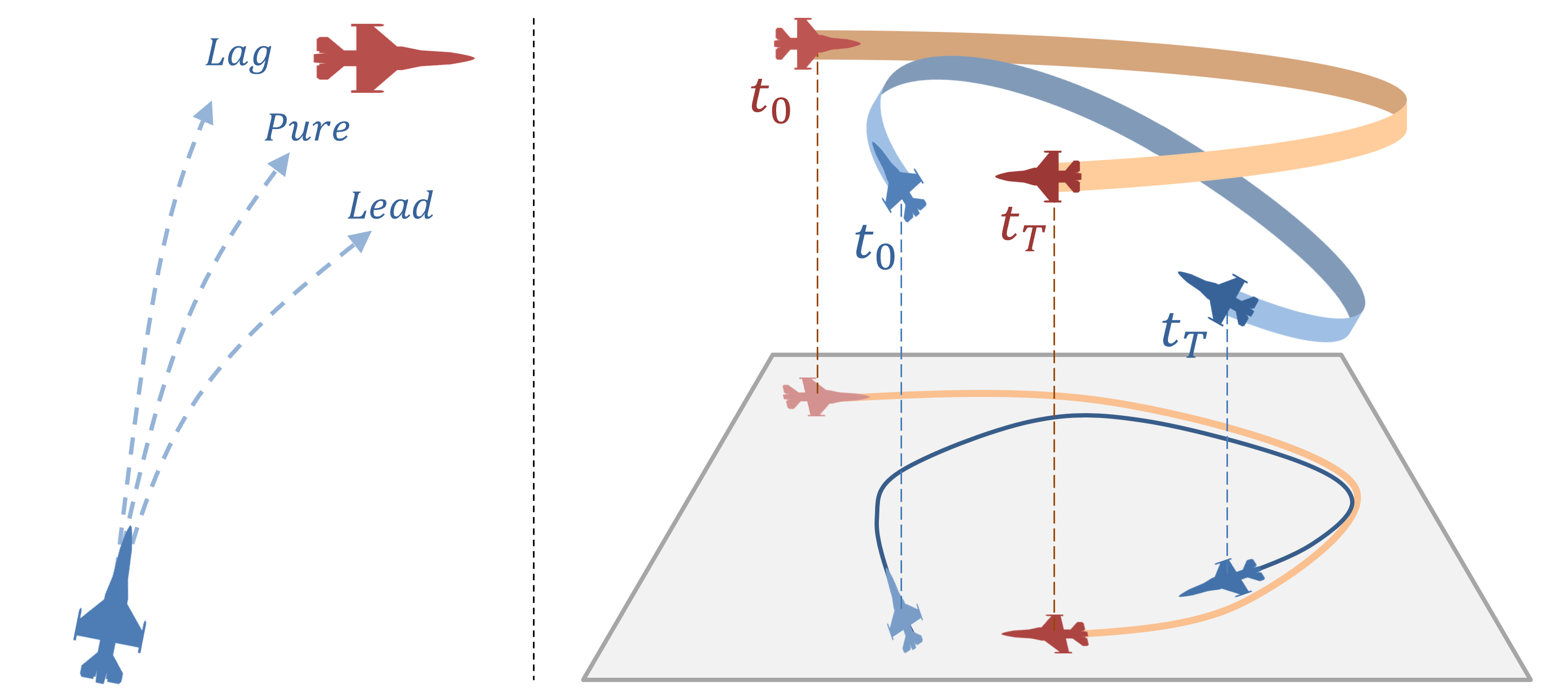
Figure 2: Human pilot’s tactical maneuvers: pursuit strategies (left) and an out-of-plane maneuver, Low Yo-Yo (right).

II-A Conventional Approaches

Based on human pilot tactics (Fig. 2) [6], most of the conventional studies used rule-based heuristics as a design approach. They proposed guidance laws with BFMs for the selection of pursuit strategies[1, 2, 3] and offensive/defensive maneuvers[4, 5] in air-to-air combat. Although heuristic-based methods were efficient in practice, they often suffered from the need for manual adjustment of parameters and flexibility issues in complex aerial environments. Several theoretical approaches utilized optimization methods, such as approximate dynamic programming (ADP) or differential game theory. The ADP provides a fast response by efficiently approximating the optimal policy[24, 25]. The differential game methods designed a scoring function matrix to generate optimal maneuvers[26, 27]. However, they often require a finite action representation for real-time computation, which is unsuitable for maneuvering in a large action space.

II-B Learning-based Approaches

Recent Deep RL-based studies can be categorized into two parts: hierarchical and end-to-end approaches. Hierarchical approaches involve a hierarchical structure with a high-level policy and a low-level controller. The policy infers discretized high-level actions in terms of maneuvers or tactics, while the controller computes low-level commands based on the actions. They construct a maneuver library[28] expanded by a set of basic control values to choose a flight maneuver[7, 8, 9, 10, 11]. Alternatively, they configure multiple sub-policies to select a proper strategy based on the current context of the combat geometry[12, 13, 14]. Despite their efficient policy optimization within a small search space, they are limited to pre-defined maneuvers and handcrafted strategies, resulting in a lack of generality. On the other hand, end-to-end methods directly map the geometry-based states into flight control actions. They design and train neural networks based on MLP[15, 16, 17, 18] or LSTM[19], which enable policy learning from experiential data and reward functions, eliminating the need for hand-designed components. However, it is less explored in the literature to develop an end-to-end policy network that can comprehend the tactical features of agile fighter jets without explicit prior knowledge.

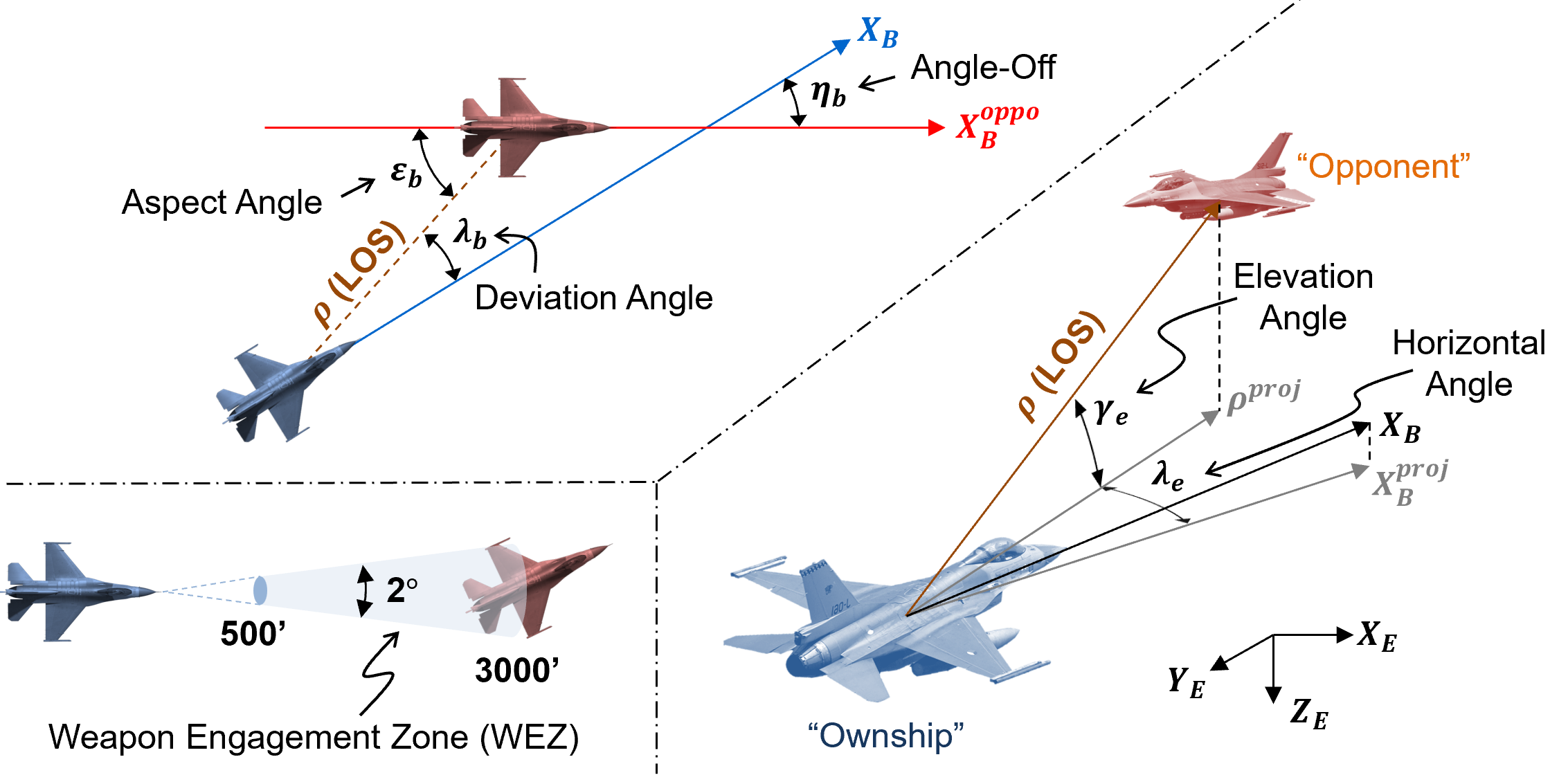
Figure 3: Geometries for aerial dogfights.

III Combat Geometries

The geometrical relationships between the aircraft in dogfights are illustrated in Fig. 3. For simplicity, the ego and opponent aircraft are referred to as the ownship and the opponent, respectively. The line-of-sight (LOS) vector $\boldsymbol{\rho}$ denotes a vector from the ownship to the opponent. The deviation and aspect angle ($\lambda_{b},\epsilon_{b}$) represent the angle between $\boldsymbol{\rho}$ and each heading vector of the ownship ($\boldsymbol{X_{b}}$) and opponent ($\boldsymbol{X^{oppo}_{b}}$), respectively. The angle-off $\eta_{b}$ indicates the angular difference between the heading vector of the ownship and opponent. We further define the horizontal and elevation deviation angles ($\lambda_{e},\gamma_{e}$) that are computed by projection with respect to the global plane $\boldsymbol{XY_{E}}$. In air combat research, the geometric area where the agent can effectively inflict damage is defined as the weapon engagement zone (WEZ), which is a two-degree spherical cone truncated at a distance range of 500 to $3,000\text{\,}\mathrm{f}\mathrm{t}$ from the ego aircraft[14].

IV Methodologies

IV-A State and Action Representation

The state space is represented by three elements: $x^{own}_{t},x^{oppo}_{t}$ and $a_{t-1}$. $x^{own}_{t}\in\mathbb{R}^{13}$ has aircraft aerodynamic states of the ownship as follows:

$$x^{own}_{t}=\{v^{b}_{x},a^{b}_{x},a^{b}_{z},\phi_{b},\theta_{b},\dot{\phi}_{b},\dot{\theta}_{b},\dot{\psi}_{b},\alpha_{b},\beta_{b},E,z_{e},v^{e}_{z}\}$$ (1)

where $v^{b}_{x}$ is the true airspeed which is aligned with the axis of the relative wind in aircraft. $a^{b}_{x},a^{b}_{z}$ are the longitudinal and vertical acceleration, and $\phi_{b},\theta_{b}$ are the roll and pitch angle in the body frame. $\dot{\phi}_{b},\dot{\theta}_{b},\dot{\psi}_{b}$ denote the rate of the roll, pitch, and yaw angle. $\alpha_{b}$ and $\beta_{b}$ indicate the angle of attack (AoA) and side slip angle. $E\!=z_{e}\!+(v^{b}_{x})^{2}/(2g)$ represents the specific energy of the ownship, where $z_{e}$ is the altitude and $g$ is the gravitational acceleration. $v^{e}_{z}$ is the vertical velocity in the earth frame. Another state element $x^{oppo}_{t}\in\mathbb{R}^{16}$ has geometric and dogfight-related state variables as

$$x^{oppo}_{t}=\{P^{bo}_{e},P^{bo}_{b},O^{bo}_{b},\lambda_{b},\epsilon_{b},\eta_{b},\lambda_{e},\gamma_{e},\xi_{own},\xi_{oppo}\},$$ (2)

where $P^{bo}_{e},P^{bo}_{b}\!\in\!\mathbb{R}^{3}$ denote the opponent’s relative position in the earth and body frame, respectively, $O^{bo}_{b}\!\in\!\mathbb{R}^{3}$ indicates the opponent’s relative orientation to the body frame. $\xi_{own},\xi_{oppo}$ refer to the life scores of the ownship and opponent. All the state elements are normalized to $[-1,1]$. We also append the previous action $a_{t-1}\!\in\!\mathbb{R}^{4}$ to the state, allowing our policy to infer the ownship’s underlying dynamics using aircraft states and past action[29]. The total features ${x}_{t}\!=\{x^{own}_{t},x^{oppo}_{t},a_{t-1}\}$ result in a 33D state space.

The action space is represented by four control commands:

$${a}_{t}=\{u_{\phi},u_{\theta},u_{\psi},u_{\tau}\}$$ (3)

where $u_{\phi},u_{\theta},u_{\psi},u_{\tau}$ specify the aileron, elevator, rudder, and thrust commands of the ownship in continuous space.

IV-B Long Short-Term Temporal Fusion Transformer

A schematic diagram of TempFuser is shown in Fig. 4. We configure long short-term state trajectories to represent tactical and dynamical state transitions. The short-term dense trajectory $s^{s}_{t}\!\in\mathbb{R}^{n_{s}\!\times 33}$ is a state history of length $n_{s}$ with a single-step interval that includes the current state $x_{t}$. Since $s^{s}_{t}$ has the same time resolution as the environment, the dense trajectory represents the dynamic state transition information (Eq. 4). On the other hand, the long-term sparse trajectory $s^{l}_{t}\!\in\mathbb{R}^{n_{l}\!\times 33}$ is a state history of length $n_{l}$ with multi-step interval $\Delta t$. It exhibits different state transitions from aircraft dynamics, containing the overall maneuver-level information (Eq. 5). In this work, we set $n_{s}\!=\!n_{l}\!=\!\Delta t\!=\!8$ to observe past state trajectories of sufficient length.

$${s}^{s}_{t} =[x_{t-(n_{s}\!-1)};x_{t-(n_{s}\!-2)};\cdots;x_{t-1};x_{t}]$$ (4)

$${s}^{l}_{t} =[x_{t-(n_{l}\!-1)\Delta t};x_{t-(n_{l}\!-2)\Delta t};\cdots;x_{t-\Delta t};x_{t}]$$ (5)

To handle the distinct temporal representations, we employ two LSTM-based input embedding pipelines. We first encode each temporal representation through a linear layer $\psi^{i}_{in}\in\mathbb{R}^{33\times d},i=\{l,s\}$ with ReLU nonlinearity. We then sequentially process each encoded trajectory feature with its corresponding LSTM. This generates hidden outputs for each trajectory, which we configure as a temporal input embedding (Eq. 6). By employing two separate LSTMs, we incorporate the sequential relational inductive bias[30] associated with both dense and sparse state transitions into the input state trajectories. As a result, the agent extracts not only the instantaneous physical properties but also the comprehensive features of the maneuvers from observations.

As all layers use the same layer size $d$, the two pipelines encode the input trajectories to long and short-term transition embeddings, $h_{l}\!\in\!\mathbb{R}^{n_{l}\!\times d}$ and $h_{s}\!\in\!\mathbb{R}^{n_{s}\!\times d}$, respectively.

$$h_{i}=\text{LSTM}(\text{ReLU}(\psi^{i}_{in}(s^{i}_{t}))),\quad i=\{l,s\}$$ (6)

We leverage a transformer encoder [21] that can learn global context to fuse two distinct transition embeddings. Before feeding the embeddings into the encoder, we concatenate them into a single sequential embedding and prepend a learnable class token $z_{class}\in\mathbb{R}^{1\times d}$. This token serves as a 1-D representation vector to summarize the sequence input and represent information about the multi-temporal state transition. Additionally, we add another learnable position embedding $z_{pos}\!\in\!\mathbb{R}^{(n_{l}+n_{s}+1)\times d}$ to the sequential embedding to provide a positional feature for each element (Eq. 7).

$$z_{0} =[z_{class};h^{1}_{l};h^{2}_{l};...;h^{n_{l}}_{l};h^{1}_{s};h^{2}_{s};...;h^{n_{s}}_{s}]+z_{pos}$$ (7)

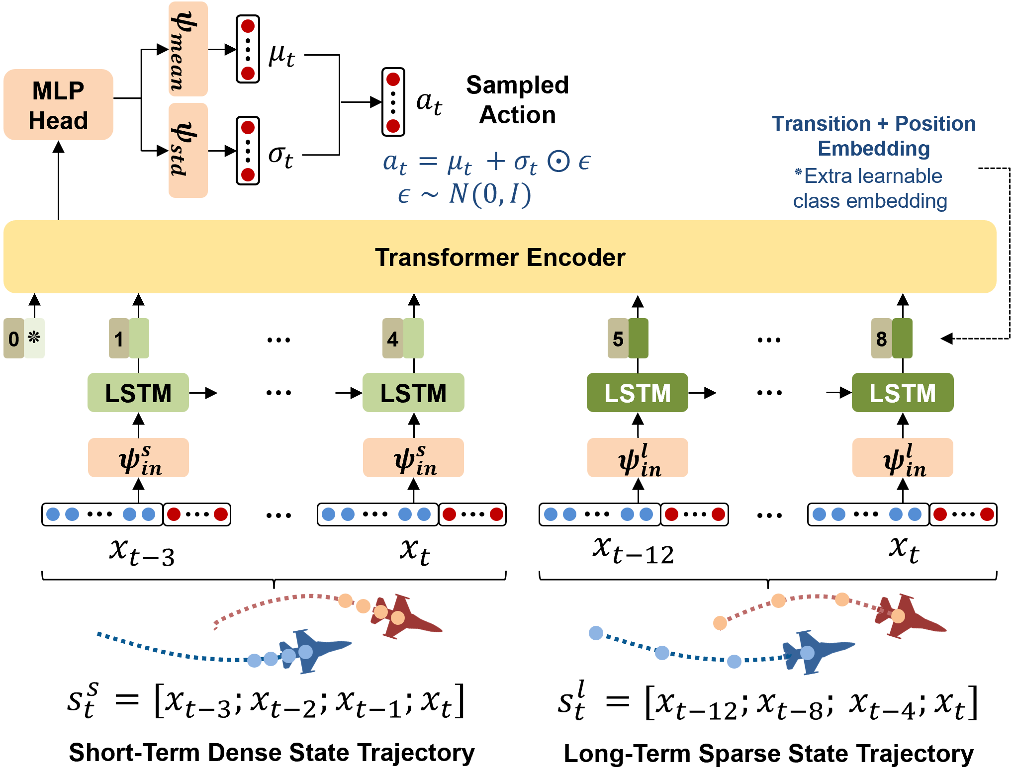
Figure 4: Overview of the TempFuser architecture for the policy network with the following example sets $n_{s}\!=\!n_{l}\!=\!\Delta t\!=\!4$.

Following [21], the transformer encoder consists of a multi-head self-attention (MSA) block and an MLP block, as well as layer normalizations (LN) and residual connections (Eq. 8, 9). The MLP has two FC layers with GeLU activation. The encoders are stacked $L$ times, increasing the capacity of the transformer network. The first element in the output of the last encoder ($z^{0}_{L}$), corresponding to the class token, is derived as the final output $y\in\mathbb{R}^{d}$ through another MLP head composed of a linear layer and LN (Eq. 10).

$$z^{\prime}_{k} =\text{MSA}(\text{LN}(z_{k-1}))+z_{k-1},\quad k=1,...,L$$ (8)

$$z_{k} =\text{MLP}(\text{LN}(z^{\prime}_{k}))+z^{\prime}_{k},\quad k=1,...,L$$ (9)

$$y =\text{MLP}(\text{LN}(z^{0}_{L}))$$ (10)

TempFuser computes the action $a_{t}\in\mathbb{R}^{4}$ in continuous space using a squashed Gaussian policy[31]. The mean and standard deviation of the action $\mu_{t},\sigma_{t}$ are computed through linear projections $\psi_{mean},\psi_{std}\in\mathbb{R}^{d\times 4}$, respectively (Eq. 11). During training, a stochastic action is sampled from these two values using the reparameterization trick of the Gaussian policy [32]. During evaluation, only the mean is used to derive a deterministic action. We use a nonlinear squashing function (tanh) for the action to be bounded within a finite range of [-1, 1] (Eq. 12).

$$\mu_{t} =\psi_{mean}(\text{LN}(y)),\quad\sigma_{t}=\psi_{std}(\text{LN}(y))$$ (11)

$${a}_{t} =\tanh{(\mu_{t}+\sigma_{t}\odot\xi)},\quad\xi\sim N(0,I).$$ (12)

IV-C Soft Actor-Critic with State Trajectories

We construct an actor-critic setup based on the Soft Actor-Critic (SAC), a sample efficient and robust off-policy algorithm [31]. The actor is our TempFuser-based policy denoted as $\pi_{\phi}$, parameterized by $\phi$. The critics are two Q-function networks: $Q_{\theta_{1}}$ and $Q_{\theta_{2}}$, parameterized by $\theta_{1}$ and $\theta_{2}$ respectively. Each Q-network has LSTM-based pipelines similar to those in the policy model. However, for training efficiency, we add layers to compute the Q-values based on a residual block[33] instead of the transformer structure.

TABLE I: Reward terms for aerial dogfights.

Reward Terms (Weight) Reward Functions Energy-Pursuit Score (2) $r_{1}=\kappa f_{p}(\lambda_{b},\left|\boldsymbol{\rho}\right|),\quad\kappa=\begin{cases}\hfil\left(1.5-E/E_{max}\right)&\hfil f_{p}<0\\ \hfil\left(0.5+E/E_{max}\right)&\hfil f_{p}\geq 0\end{cases}$ Horizontal Pursuit (1) $r_{2}=-\lambda_{e}/180\degree$ WEZ (Ownship, Opponent) (5) $r_{3}=\begin{cases}\hfil+1&\boldsymbol{\rho}\in\text{WEZ}_{own}\\ \hfil 0&\boldsymbol{\rho}\notin\text{WEZ}_{own}\end{cases}$, $r_{4}=\begin{cases}\hfil-1&\boldsymbol{\rho}\in\text{WEZ}_{oppo}\\ \hfil 0&\boldsymbol{\rho}\notin\text{WEZ}_{oppo}\end{cases}$ Specific Energy (0.5) $r_{5}=clip((E-E_{mid})/E_{mid},-1,+1)$ Altitude (15) $r_{6}=\left(0.5\left(1-\text{min}(0,{v}_{z}/{v}_{max})\right)\times\text{min}\left(0,\frac{z-z_{low}}{z_{low}-z_{min}}\right)\right)^{3}$ AoA (1) $r_{7}=\begin{cases}\hfil-\left|\alpha_{b}\right|/45\degree&\alpha_{b}<0\degree\\ \hfil 0&0\degree\leq\alpha_{b}<45\degree\\ \hfil-(\alpha_{b}-45\degree)/45\degree&\alpha_{b}\geq 45\degree\end{cases}$

Algorithm 1 summarizes the overall training process. At each episode, a fixed-size FIFO buffer $\mathcal{T}$ is initialized with $n_{l}\Delta t$ states observed through actions $a_{init}$ in the environment. In each step, the state trajectories $s^{l}_{t},s^{s}_{t}$ are indexed from the buffer $\mathcal{T}$. The trajectories are then fed to the policy $\pi_{\phi}$ to sample an action $a_{t}$ for interacting with the environment. After the agent observes the next states $x^{own}_{t+1},x^{oppo}_{t+1}$ and reward $r_{t}$, the oldest state is dequeued and $x_{t+1}\!=\{x^{own}_{t+1},x^{oppo}_{t+1},a_{t}\}$ is enqueued in $\mathcal{T}$. New state trajectories are indexed from the updated buffer, and the transition data is stored in a replay buffer $D$. During the update phase, The model parameters ($\theta_{1},\theta_{2},\phi$) with the temperature $\alpha$ are updated with the objective functions $J_{Q}(\theta_{1})$, $J_{Q}(\theta_{2})$, $J_{\pi}(\phi)$ and $J_{\alpha}(\alpha)$. The weight of the target Q-functions $\bar{\theta}_{1},\bar{\theta}_{2}$ are updated by Polyak Averaging[34] with a coefficient $\tau$.

IV-D Reward Function

The reward function $r_{t}$ is a weighted summation of the terms described in Table I. Overall, the reward encourages the agent to maximize the energy-pursuit score ($r_{1}$), enhance horizontal pursuit performance ($r_{2}$), position the enemy within the ownship’s WEZ ($r_{3}$), and avoid the enemy’s WEZ ($r_{4}$), all while managing $E$ close to the desired energy $E_{des}$ ($r_{5}$). Concurrently, it motivates the agent to maneuver within a safe altitude ($r_{6}$) and the proper AoA ranges ($r_{7}$), preventing crashes and aerodynamic stalls.

Algorithm 1 SAC Training Algorithm with State Trajectories

Input: $\phi,\theta_{1},\theta_{2}$
Output: Optimized parameters $\phi,\theta_{1},\theta_{2}$

1:$\bar{\theta}_{1}\leftarrow\theta_{1},\bar{\theta}_{2}\leftarrow\theta_{2},D\leftarrow\emptyset,\mathcal{T}^{\dagger}\leftarrow\emptyset$

2:for each episode do

3:    while $n_{l}\Delta t$ steps do

4:         Execute action ${a}_{init}$ and observe $x^{own}_{t+1},x^{oppo}_{t+1},r_{t}$

5:         $\mathcal{T}.\text{enqueue}(\{x^{own}_{t+1},x^{oppo}_{t+1},a_{init}\})$     

6:    Initialize ${s}^{s}_{t},{s}^{l}_{t}$ by indexing from $\mathcal{T}$

7:    while not done do

8:         ${a}_{t}\sim\pi_{\phi}({a}_{t}|{s}^{s}_{t},{s}^{l}_{t})$

9:         Execute action ${a}_{t}$ and observe $x^{own}_{t+1},x^{oppo}_{t+1},r_{t}$

10:         $\mathcal{T}.\text{dequeue}()$ and $\mathcal{T}.\text{enqueue}(\{x^{own}_{t+1},x^{oppo}_{t+1},a_{t}\})$

11:         ${s}^{s}_{t+1}\leftarrow\{\mathcal{T}[n_{l}\Delta t\!-(n_{s}\!-1)];\mathcal{T}[n_{l}\Delta t\!-(n_{s}\!-2)];\cdots;\newline \hskip 54.00009pt\mathcal{T}[n_{l}\Delta t-1];\mathcal{T}[n_{l}\Delta t]\}$

12:         ${s}^{l}_{t+1}\!\leftarrow\{\mathcal{T}[\Delta t];\mathcal{T}[2\Delta t];\cdots;\mathcal{T}[(n_{l}\!-1)\Delta t];\mathcal{T}[n_{l}\Delta t]\}$

13:         $D\leftarrow D\cup\{({s}^{s}_{t},{s}^{l}_{t},{a}_{t},r_{t},{s}^{s}_{t+1},{s}^{l}_{t+1})\}$

14:         ${s}^{s}_{t}\leftarrow{s}^{s}_{t+1},{s}^{l}_{t}\leftarrow{s}^{l}_{t+1}$     

15:    for each gradient step do

16:         $\theta_{i}\leftarrow\theta_{i}-\lambda_{Q}\nabla_{\theta_{i}}J_{Q}(\theta_{i})$ for $i\in\{1,2\}$

17:         $\phi\leftarrow\phi-\lambda_{\pi}\nabla_{\phi}J_{\pi}(\phi),\ \alpha\leftarrow\alpha-\lambda_{\alpha}\nabla_{\alpha}J_{\alpha}(\alpha)$

18:         $\bar{\theta}_{i}\leftarrow\tau\theta_{i}+(1-\tau)\bar{\theta}_{i}$ for $i\in\{1,2\}$     

19:^†The index of $\mathcal{T}$ is started from 1.

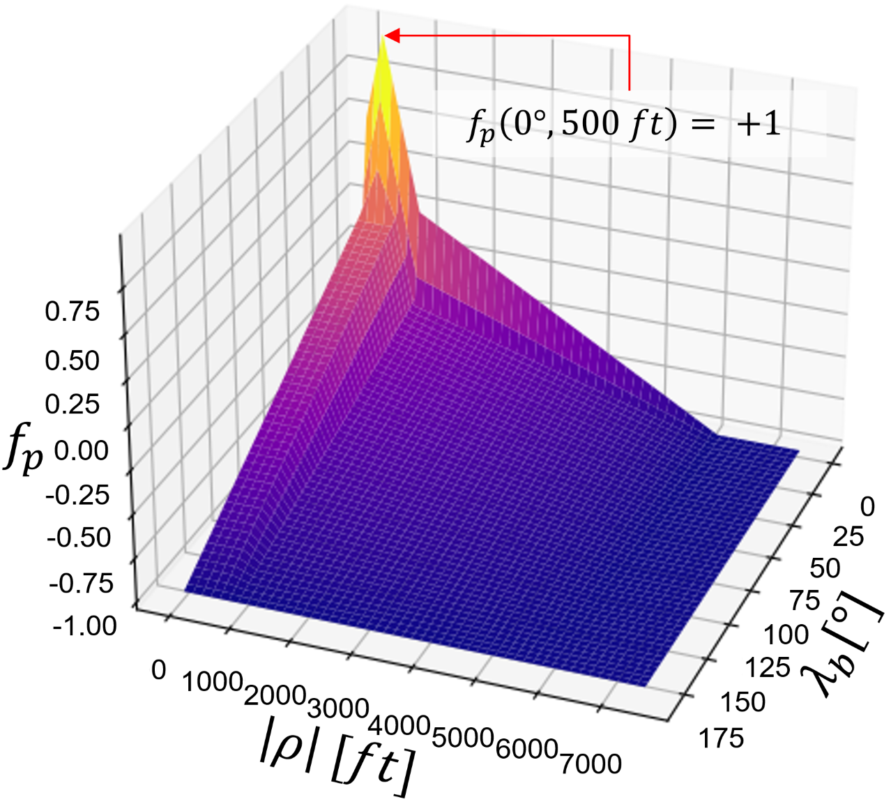
Figure 5: Pursuit score function.

The energy-pursuit score consists of a pursuit score function $f_{p}$ (Fig. 5) and a factor $\kappa$. The function assigns higher scores to deviation angles ($\lambda_{b}$) closer to zero and relative distances ($\left|\boldsymbol{\rho}\right|$) closer to the desired distance ($500\text{\,}\mathrm{f}\mathrm{t}$) inside the WEZ. $\kappa$ is determined by the sign of $f_{p}$ and scales the magnitude of $r_{1}$ by $E$. This energy-embedded pursuit score incentivizes the agent to effectively maintain sufficient specific energy by managing potential and kinetic energy when tracking the opponent.

The altitude reward activates from $z_{low}\!=\!$1,000\text{\,}\mathrm{f}\mathrm{t}$$ to prevent the agent from descending below $z_{min}\!=\!$250\text{\,}\mathrm{f}\mathrm{t}$$. Inspired by the collision term in [35], we design the penalty to become more severe as the size of the negative vertical velocity ($v_{z}$) increases. This encourages the agent to reduce its descent rate when entering low altitude areas.

V Experiment

TABLE II: Quantitative Evaluation against 4 Opponents (F-15E, F-16, F/A-18, Su-27) and an Unseen Aircraft (Su-30)

v.s. F-15E v.s. F-16 v.s. F/A-18 v.s. Su-27 v.s. Su-30 Method Win (%) $\uparrow$ Loss (%) $\downarrow$ Damage (%) $\uparrow$ Life (%) $\uparrow$ Win (%) $\uparrow$ Loss (%) $\downarrow$ Damage (%) $\uparrow$ Life (%) $\uparrow$ Win (%) $\uparrow$ Loss (%) $\downarrow$ Damage (%) $\uparrow$ Life (%) $\uparrow$ Win (%) $\uparrow$ Loss (%) $\downarrow$ Damage (%) $\uparrow$ Life (%) $\uparrow$ Win (%) $\uparrow$ Loss (%) $\downarrow$ Damage (%) $\uparrow$ Life (%) $\uparrow$ DCS-Ace 34.6 43.0 38.9 54.4 38.3 39.6 38.8 59.1 18.7 58.0 32.9 32.3 22.9 41.8 37.0 52.7 9.2 66.4 19.2 28.6 MLP 37.3 58.5 38.2 40.2 3.7 87.6 4.6 10.1 6.5 85.1 8.2 10.8 1.7 31.3 3.8 53.3 5.7 72.4 7.3 20.0 LSTM 88.6 10.9 91.8 89.0 28.6 64.2 38.5 34.9 83.8 15.4 88.5 79.4 55.7 35.3 67.2 60.0 60.4 39.3 71.3 58.5 LS-LSTM 83.3 16.7 86.7 78.2 75.6 20.1 83.2 77.5 88.1 11.7 90.8 87.0 82.6 14.4 85.9 77.0 62.4 36.8 69.7 60.3 TempFuser 93.5 6.5 94.2 92.5 86.3 13.4 96.0 86.6 89.1 10.9 90.3 86.2 92.5 7.0 95.1 92.0 86.1 13.9 90.8 81.2

V-A Environment Setup

We configured dogfight scenarios using DCS that has high-fidelity flight dynamics and a range of mission configuration tools. We selected the F-16 for our agent, which is an example of a mature fighter jet.

Figure 6: Mission scenarios.

Fig. 6 shows scenario configurations with spawn points and directions. In training episodes, our agent (blue) was initialized with an altitude of $15,000\text{\,}\mathrm{f}\mathrm{t}$ and a speed of $500\text{\,}\mathrm{k}\mathrm{t}$, and the opponent (red), with different altitudes ($10,000\text{\,}\mathrm{-}$$18,000\text{\,}\mathrm{f}\mathrm{t}$), was randomly spawned with various locations within $30,000\text{\,}\mathrm{f}\mathrm{t}$ from our agent. In the evaluation, the ownship and opponent were spawned facing each other at a distance of $10,000\text{\,}\mathrm{f}\mathrm{t}$, participating in episodes designed to facilitate fair performance comparisons. Each episode was reset under the following conditions: 1) if the altitude of any agent fell below $z_{min}$, 2) if the life of any agent dropped to 0, 3) if the ownship reached a maximum of 9,000 time steps, or 4) if agents collided with each other.

We set up various opponent fighter jets as depicted in Fig. 7. In training, the opponent was randomly selected from four aircraft: one with equivalent aerodynamic specifications (F-16), two with comparable specifications (F-15E, F/A-18A), and one with superior specifications (Su-27) compared to our agent’s aircraft[23]. Alongside the four aircraft, we additionally spawned the Su-30 in evaluation, which had not been encountered during training, to assess the robustness of our policy against a new opponent.

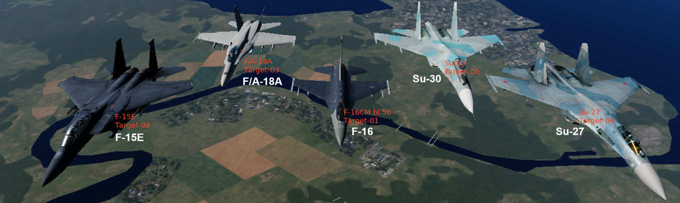
Figure 7: Different types of aircraft for the opponent in DCS.

V-B Baseline Schemes

• DCS-Ace: This is a built-in AI model with the most challenging pilot skill, Ace, in the DCS simulator [22].

• MLP: This is a multilayer perceptron network that observes only the current state $x_{t}$ (akin to [17]).

• LSTM: This considers the short-term state trajectory $s^{s}_{t}$ only based on an LSTM layer (similar to [19]).

• LS-LSTM: This scheme employs the long short-term temporal input embeddings using $s^{l}_{t},s^{s}_{t}$, but consists only of LSTM layers without the transformer encoder.

V-C Evaluation

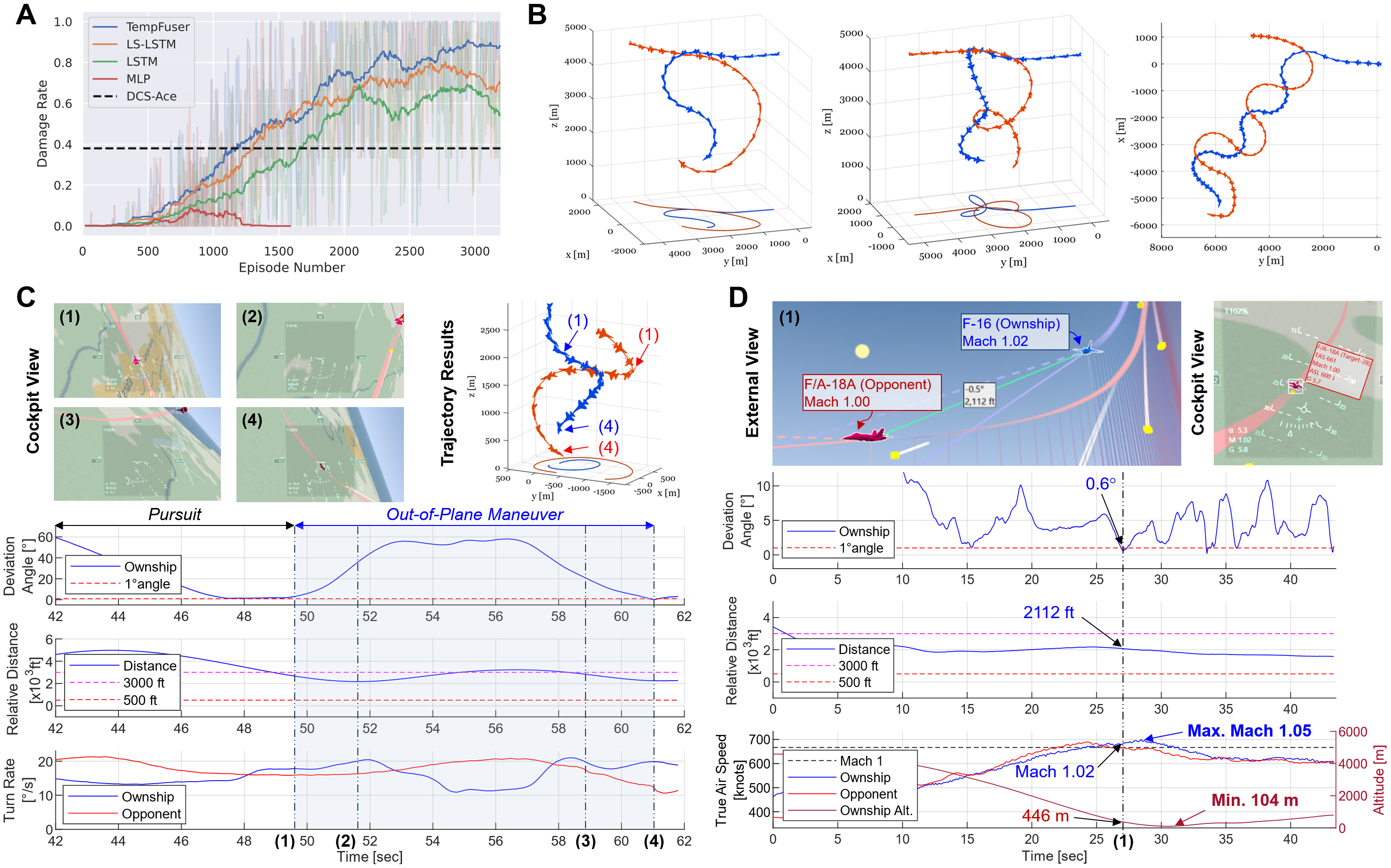
Figure 8: Evaluation results. (A): Learning curves of the normalized damage rate against the opponent. (B): Results of engagements against the opponent (left: F-15E, middle: F-16, right: Su-27). 3D flight and horizontally projected trajectories of the ownship (blue) and opponent (red) are illustrated from the beginning until the winning moment. (C): Quantitative results of learned tactical out-of-plane maneuvers against a superior-spec aircraft (Su-30). (D): Quantitative results of a near-sonic speed scenario against the F/A-18A opponent. All the cockpit and external views are visualized by Tacview[36].

Learning Curves: We evaluated learning curves across different policies using the WEZ damage ratio. This ratio signifies the proportion of the opponent’s life that our agent has reduced through the use of WEZ. Fig. 8 (A) compares the performance of different baseline policies. The results show that our model surpasses other baseline models in terms of learning speed and convergence. The MLP was unable to learn the appropriate maneuvers to confront aggressive opponents. While the LSTM successfully learned aerial dogfights and achieved a damage rate of over $50\%$, its performance plateaued at around $60\%$. By employing the long and short-term features, the LS-LSTM exhibited better performance than the LSTM. However, as it only concatenates the two features without adequately integrating them, it failed to fully leverage their combined potential, preventing it from surpassing the $80\%$ performance threshold. By incorporating the transformer architecture, TempFuser effectively captured the opponent’s tactical and dynamic attributes, resulting in an average WEZ damage of $90\%$.

Quantitative Performance: Table II summarizes the performance of the different policies against the four types of aircraft and an unseen aircraft, the Su-30. We use four quantitative evaluation metrics: win rate (Win), loss rate (Loss), WEZ damage rate (Damage), and ownship’s life score rate (Life). Each metric is calculated as an average of 400 episode results. Our model generally outperforms other baseline models in terms of win and damage rates. The non-learning DCS-Ace often fell short of achieving a conclusive outcome (win/loss) and struggled against fighters with higher aerodynamic specifications (Su-27, Su-30). When it comes to the learnable models, the F-16, Su-27, and Su-30 aircraft pose the greatest challenge as opponents, as the aerodynamic specifications of the ownship are either equal to or lower than those of the opponent. Only the models that incorporate both long and short-term trajectory inputs (LS-LSTM, TempFuser) demonstrate remarkable successes, achieving a win/damage rate of over $50\%$ against the various types of opponents, including those challenging aircraft. However, the performance of the LS-LSTM notably diminished against the unobserved opponent (Su-30), with win/damage rates falling to around $60\%$. Our TempFuser, on the other hand, exhibits only a minor performance decrement while effectively reducing the opponent’s life score by an average of $90\%$, achieving the highest win rate ($86\%$) and life rate ($81\%$).

V-D Learned Flight Behavior

Basic Flight Maneuvers: Fig. 8 (B) shows the flight trajectories of our agent against the three different opponents (F-15E, F-16, Su-27) during engagements. The overall results show that our method successfully learns the maneuverability of fighter jets, enabling it to perform faster turning maneuvers and secure an advantage through complex combinations of the four control commands. Fig. 8 (B, left) illustrates the result of an episode against an F-15E opponent. While the opponent performed with an average turn rate of $7.85\text{\,}\mathrm{\SIUnitSymbolDegree}$/s (max. $16.80\text{\,}\mathrm{\SIUnitSymbolDegree}$/s), our agent showed a more rapid average turn rate of $11.18\text{\,}\mathrm{\SIUnitSymbolDegree}$/s (max. $26.41\text{\,}\mathrm{\SIUnitSymbolDegree}$/s), enabling it to quickly gain a favorable position and outperform the enemy agent.

Furthermore, our agent demonstrated strategic reactive behavior against the opponent performing complex turns. Fig. 8 (B, middle) depicts a scenario with the F-16 opponent, which is the same aircraft as our agent. When the opponent performed two turning descents, our model responded by executing a spiral dive with a tighter radius and faster turning speed, eventually winning the scenario by targeting the anticipated area where the enemy was expected to reach. As another scenario, Fig. 8 (B, right) displays the results against an aggressive opponent (Su-27). With superior aerodynamic properties compared to the ownship, the Su-27 performed high-speed flight maneuvers, making pursuit challenging. In response, our TempFuser-based agent executed Flat Scissors-like maneuvers[6], intersecting the opponent’s trajectory and effectively targeting the fast-moving aircraft.

Tactical Flight Maneuvers: Without explicit prior knowledge, our method discovers and learns tactical maneuvers that are close to the human pilot’s skills depicted in Fig. 2. Fig. 8 (C) illustrates the results of an engaging situation against the Su-30. Our method executed pursuit maneuvers until 49.7 sec, reducing the tracking error and relative distance by up to $1.4\text{\,}\mathrm{\SIUnitSymbolDegree}$and $2,621\text{\,}\mathrm{f}\mathrm{t}$ ((1) in C). However, the pursuit method alone was not able to place the Su-30, which has a faster average speed of $496\text{\,}\mathrm{k}\mathrm{t}$ ($919\text{\,}\mathrm{k}\mathrm{m}\mathrm{/}\mathrm{h}$), in the effective damage zone of our F-16. To overcome this situation, our method demonstrated an out-of-plane maneuver that leveraged gravity assistance to perform a rapid turn toward the anticipated path of the opponent, despite the increased tracking angle error ((1-4) in C). Those tactical maneuvers enabled our agent to stay within the opponent’s turning circle while keeping the distance within $500\text{\,}\mathrm{-}$$3,000\text{\,}\mathrm{f}\mathrm{t}$, even against the faster opponent. Moreover, our agent achieved a more rapid instantaneous turn rate ($20.97\text{\,}\mathrm{\SIUnitSymbolDegree}$/s) than the opponent, strategically placing it within our aircraft’s WEZ ((4) in C).

Robust Pursuit in Supersonic Speed: We further investigated the robustness of the policy in aggressive scenarios, specifically at supersonic speeds. Fig. 8 (D) illustrates an aerial scene with overall quantitative results where our agent tracked an F/A-18A opponent evading to a low altitude with near-supersonic velocity. As the deviation angle decreased, the opponent increased its speed by descending to an altitude below $500\text{\,}\mathrm{f}\mathrm{t}$. Against such a high-speed adversary, our agent maintained the desired distance while traveling at Mach 1.02 and reduced the deviation angle by up to 0.6°. It then executed high-speed pursuit up to Mach 1.05 at a critically low altitude while keeping the proper distance within the WEZ range (near $2,000\text{\,}\mathrm{f}\mathrm{t}$). Finally, it won against the adversary by accumulating damage. These results show the robustness of our policy model to aim the agile opponent in supersonic situations while considering safe altitude requirements.

VI Conclusion

We introduced TempFuser, a long short-term temporal fusion transformer designed for aerial dogfights. Our model integrates both long and short-term trajectory representations to effectively capture the tactics and dynamic-level features of agile fighter jets engaged in aggressive combat scenarios. In high-fidelity airborne scenarios, the proposed model outperforms other baseline methods, across a diverse range of opponent aircraft types. Our model successfully learns tactical flight maneuvers and robust pursuit strategies without relying on heuristic knowledge.

We believe our work has potential for broader applications beyond dogfights. It could be extended to other agile and interactive scenarios, such as autonomous racing, where understanding the strategies of other aggressive agents is crucial. In future research, we aim to adapt our method to these fields, as well as to enhance it for multi-agent scenarios beyond the one-versus-one context.

References

- [1] G. H. Burgin and L. Sidor, “Rule-based air combat simulation,” Tech. Rep., 1988.
- [2] D.-I. You and D. H. Shim, “Design of an aerial combat guidance law using virtual pursuit point concept,” Proceedings of the Institution of Mechanical Engineers, Part G: Journal of Aerospace Engineering, vol. 229, no. 5, pp. 792–813, 2015.
- [3] N. Ramírez López and R. Żbikowski, “Effectiveness of autonomous decision making for unmanned combat aerial vehicles in dogfight engagements,” Journal of Guidance, control, and Dynamics, vol. 41, no. 4, pp. 1021–1024, 2018.
- [4] H. Shin, J. Lee, D. H. Shim, and D.-I. You, “Design of a virtual fighter pilot and simulation environment for unmanned combat aerial vehicles,” in AIAA Guidance, Navigation, and Control Conference, 2017, p. 1027.
- [5] H. Shin, J. Lee, H. Kim, and D. H. Shim, “An autonomous aerial combat framework for two-on-two engagements based on basic fighter maneuvers,” Aerospace Science and Technology, vol. 72, pp. 305–315, 2018.
- [6] R. L. Shaw, “Fighter combat,” Tactics and Maneuvering; Naval Institute Press: Annapolis, MD, USA, 1985.
- [7] X. Zhang, G. Liu, C. Yang, and J. Wu, “Research on air confrontation maneuver decision-making method based on reinforcement learning,” Electronics, vol. 7, no. 11, p. 279, 2018.
- [8] Q. Yang, J. Zhang, G. Shi, J. Hu, and Y. Wu, “Maneuver decision of uav in short-range air combat based on deep reinforcement learning,” IEEE Access, vol. 8, pp. 363–378, 2019.
- [9] D. Hu, R. Yang, J. Zuo, Z. Zhang, J. Wu, and Y. Wang, “Application of deep reinforcement learning in maneuver planning of beyond-visual-range air combat,” IEEE Access, vol. 9, pp. 32 282–32 297, 2021.
- [10] Z. Fan, Y. Xu, Y. Kang, and D. Luo, “Air combat maneuver decision method based on a3c deep reinforcement learning,” Machines, vol. 10, no. 11, p. 1033, 2022.
- [11] J. Hu, L. Wang, T. Hu, C. Guo, and Y. Wang, “Autonomous maneuver decision making of dual-uav cooperative air combat based on deep reinforcement learning,” Electronics, vol. 11, no. 3, p. 467, 2022.
- [12] Z. Yang, D. Zhou, H. Piao, K. Zhang, W. Kong, and Q. Pan, “Evasive maneuver strategy for ucav in beyond-visual-range air combat based on hierarchical multi-objective evolutionary algorithm,” IEEE Access, vol. 8, pp. 46 605–46 623, 2020.
- [13] H. Piao, Z. Sun, G. Meng, H. Chen, B. Qu, K. Lang, Y. Sun, S. Yang, and X. Peng, “Beyond-visual-range air combat tactics auto-generation by reinforcement learning,” in 2020 International Joint Conference on Neural Networks (IJCNN), 2020, pp. 1–8.
- [14] A. P. Pope, J. S. Ide, D. Mićović, H. Diaz, D. Rosenbluth, L. Ritholtz, J. C. Twedt, T. T. Walker, K. Alcedo, and D. Javorsek, “Hierarchical reinforcement learning for air-to-air combat,” in 2021 international conference on unmanned aircraft systems (ICUAS). IEEE, 2021, pp. 275–284.
- [15] Q. Yang, Y. Zhu, J. Zhang, S. Qiao, and J. Liu, “Uav air combat autonomous maneuver decision based on ddpg algorithm,” in 2019 IEEE 15th international conference on control and automation (ICCA). IEEE, 2019, pp. 37–42.
- [16] W. Kong, D. Zhou, Z. Yang, K. Zhang, and L. Zeng, “Maneuver strategy generation of ucav for within visual range air combat based on multi-agent reinforcement learning and target position prediction,” Applied Sciences, vol. 10, no. 15, p. 5198, 2020.
- [17] J. Yoo, H. Seong, D. H. Shim, J. H. Bae, and Y.-D. Kim, “Deep reinforcement learning-based intelligent agent for autonomous air combat,” in 2022 IEEE/AIAA 41st Digital Avionics Systems Conference (DASC). IEEE, 2022, pp. 1–9.
- [18] L. Li, Z. Zhou, J. Chai, Z. Liu, Y. Zhu, and J. Yi, “Learning continuous 3-dof air-to-air close-in combat strategy using proximal policy optimization,” in 2022 IEEE Conference on Games (CoG). IEEE, 2022, pp. 616–619.
- [19] J. H. Bae, H. Jung, S. Kim, S. Kim, and Y.-D. Kim, “Deep reinforcement learning-based air-to-air combat maneuver generation in a realistic environment,” IEEE Access, vol. 11, pp. 26 427–26 440, 2023.
- [20] S. Hochreiter and J. Schmidhuber, “Long short-term memory,” Neural computation, vol. 9, no. 8, pp. 1735–1780, 1997.
- [21] A. Dosovitskiy, L. Beyer, A. Kolesnikov, D. Weissenborn, X. Zhai, T. Unterthiner, M. Dehghani, M. Minderer, G. Heigold, S. Gelly et al., “An image is worth 16x16 words: Transformers for image recognition at scale,” arXiv preprint arXiv:2010.11929, 2020.
- [22] Eagle Dynamics, “Digital combat simulator world,” 2023, accessed: 2023-08-24. [Online]. Available: https://www.digitalcombatsimulator.com
- [23] A. Bongers and J. L. Torres, “Measuring technological trends: A comparison between us and ussr/russian jet fighter aircraft,” Technological Forecasting and Social Change, vol. 87, pp. 125–134, 2014.
- [24] J. S. McGrew, J. P. How, B. Williams, and N. Roy, “Air-combat strategy using approximate dynamic programming,” Journal of guidance, control, and dynamics, vol. 33, no. 5, pp. 1641–1654, 2010.
- [25] M. Wang, L. Wang, T. Yue, and H. Liu, “Influence of unmanned combat aerial vehicle agility on short-range aerial combat effectiveness,” Aerospace Science and Technology, vol. 96, p. 105534, 2020.
- [26] M. Ardema and N. Rajan, “An approach to three-dimensional aircraft pursuit–evasion,” in Pursuit-Evasion Differential Games. Elsevier, 1987, pp. 97–110.
- [27] H. Park, B.-Y. Lee, M.-J. Tahk, and D.-W. Yoo, “Differential game based air combat maneuver generation using scoring function matrix,” International Journal of Aeronautical and Space Sciences, vol. 17, no. 2, pp. 204–213, 2016.
- [28] F. Austin, G. Carbone, M. Falco, H. Hinz, and M. Lewis, “Game theory for automated maneuvering during air-to-air combat,” Journal of Guidance, Control, and Dynamics, vol. 13, no. 6, pp. 1143–1149, 1990.
- [29] X. B. Peng, M. Andrychowicz, W. Zaremba, and P. Abbeel, “Sim-to-real transfer of robotic control with dynamics randomization,” in 2018 IEEE international conference on robotics and automation (ICRA). IEEE, 2018, pp. 1–8.
- [30] P. W. Battaglia, J. B. Hamrick, V. Bapst, A. Sanchez-Gonzalez, V. Zambaldi, M. Malinowski, A. Tacchetti, D. Raposo, A. Santoro, R. Faulkner et al., “Relational inductive biases, deep learning, and graph networks,” arXiv preprint arXiv:1806.01261, 2018.
- [31] T. Haarnoja, A. Zhou, K. Hartikainen, G. Tucker, S. Ha, J. Tan, V. Kumar, H. Zhu, A. Gupta, P. Abbeel et al., “Soft actor-critic algorithms and applications,” arXiv preprint arXiv:1812.05905, 2018.
- [32] J. Schulman, N. Heess, T. Weber, and P. Abbeel, “Gradient estimation using stochastic computation graphs,” arXiv preprint arXiv:1506.05254, 2015.
- [33] K. He, X. Zhang, S. Ren, and J. Sun, “Deep residual learning for image recognition,” in Proceedings of the IEEE conference on computer vision and pattern recognition, 2016, pp. 770–778.
- [34] B. T. Polyak and A. B. Juditsky, “Acceleration of stochastic approximation by averaging,” SIAM journal on control and optimization, vol. 30, no. 4, pp. 838–855, 1992.
- [35] H. Seong, C. Jung, S. Lee, and D. H. Shim, “Learning to drive at unsignalized intersections using attention-based deep reinforcement learning,” in 2021 IEEE International Intelligent Transportation Systems Conference (ITSC). IEEE, 2021, pp. 559–566.
- [36] R. Software, “Tacview - the universal flight data analysis tool,” 2023, accessed: 2023-08-24. [Online]. Available: http://www.tacview.net/