Imbalanced Large Graph Learning Framework for FPGA Logic Elements Packing Prediction

Abstract

Packing is a required step in a typical FPGA CAD flow. It has high impacts to the performance of FPGA placement and routing. Early prediction of packing results can guide design optimization and expedite design closure. In this work, we propose an imbalanced large graph learning framework, ImLG, for prediction of whether logic elements will be packed after placement. Specifically, we propose dedicated feature extraction and feature aggregation methods to enhance the node representation learning of circuit graphs. With imbalanced distribution of packed and unpacked logic elements, we further propose techniques such as graph oversampling and mini-batch training for this imbalanced learning task in large circuit graphs. Experimental results demonstrate that our framework can improve the F1 score by 42.82% compared to the most recent Gaussian-based prediction method. Physical design results show that the proposed method can assist the placer in improving routed wirelength by 0.93% and SLICE occupation by 0.89%.

I Introduction

In a typical FPGA CAD flow, packing clusters all the low-level logic elements such as lookup tables (LUTs) and flip-flops (FFs) into the basic operational objects, i.e., basic logic elements (BLEs) in configurable logic blocks (CLBs) for the placement, as shown in Fig. 1. Packing is usually performed during placement and routing (P&R), and its quality has high impacts on the P&R closure.

State-of-the-art (SOTA) FPGA placement algorithms [1]–[4] require packing prediction in the optimization iterations for logic resource estimation. [1] and [2] propose to predict packing by setting static empirical resource demands, which has poor generalization among designs. [3] and [4] propose a Gaussian-based approach for packing prediction through estimating resource demands. Despite its effectiveness, the previous approaches have two major drawbacks. Firstly, resource demands alone are not enough to decide whether an instance can be packed or not. Secondly, as the number of packed elements is much larger than that of unpacked ones, these approaches are not able to capture the imbalanced distribution of packing results, causing low accuracy on predicting unpacked elements, i.e., high false positive rates.

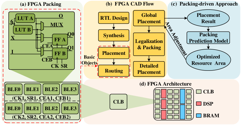
Figure 1: The packing-driven FPGA CAD flow.

As an FPGA design can be represented as a circuit graph, packing prediction can be viewed as a graph learning task on large circuit graphs with physical information and imbalanced label distribution on nodes. Recent studies have shown promising results of leveraging graph neural networks (GNNs) for related tasks like routing congestion prediction in physical design [6] – [8]. Inspired by these works, in this work, we propose an imbalanced large graph learning framework for packing prediction of logic elements in the FPGA desgin flow. Different from routing congestion prediction, packing prediction is more challenging since the operational objects in this task are instance-level logic elements with complex netlists and imbalanced distribution of packing labels.

The key contributions are summarized as follows.

• We propose a new graph learning based paradigm for FPGA packing prediction with graph oversampling and mini-batch training to handle imbalanced distribution of packed and unpacked elements.

• We propose a region-encoding based feature extraction scheme that aligns with the local nature of packing process.

• We propose a homophily-aware feature aggregation method to capture the differences between packed elements and unpacked ones, which enhances the quality of embeddings.

Detailed experiments demonstrate that our framework outperforms the most recent Gaussian-based method in prediction accuracy. And this technique improves the routed wirelength by 0.93% and the SLICE occupation by 0.89% for physical design.

The rest of the paper is organized as follows. Section II introduces the background and overview. Section III provides the proposed framework. Section IV demonstrates the results. Section V concludes the paper.

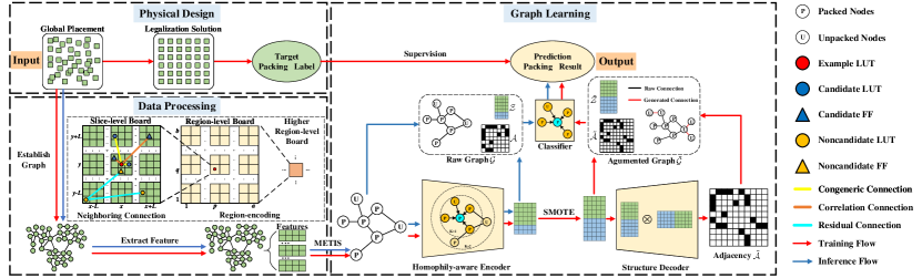
Figure 2: Proposed imbalanced large graph learning framework.

II Preliminaries and Overview

II-A FPGA Architecture

To detail the FPGA architecture, a typical architecture Xilinx UltraScale VU095 is illustrated in Fig. 1, in which a CLB slice contains eight BLEs and each BLE further contains two LUTs and FFs. The LUTs or FFs satisfying constraints are packed into the high-level BLEs. And each CLB is composed of LUTs and FFs with specific logical constraints.

II-B Imbalanced Graph Learning for Binary Classification

Given the packing prediction can be modeled as a binary node classification task on an imbalanced graph $\mathcal{G}_{im}$, where the number of packed elements is much larger than that of unpacked ones by more than $10:1$. Such biased data greatly weaken the classification performance of the GNN model. The current SOTA methods, such as [15][16], solve this problem with data oversampling algorithms, as it has been found to be the most effective and stable solution. These methods aim to balance the raw data distribution for achieving good classification performance on the augmented balanced graph.

II-C Packing Prediction in elfPlace

In elfPlace, legalization and packing are carried out simultaneously. Therefore, in the global placement stage, elfPlace performs a Gaussian method to predict packing results by estimating resource demands and thus assigning appropriate resources for each instance. This packing-driven approach has the ability to enhance circuit quality. However, considering the low prediction accuracy of the Gaussian method, a better packing prediction paradigm will be proposed to assist the placer to achieve better solution.

II-D Overview of Proposed Framework

The overall framework is depicted in Fig. 2, which consists of physical design, data processing, and graph learning. The red row represents the training flow, while the blue row represents the inference flow.

The physical design generates the target packing labels through a legalization process. This part is only performed in the training stage. Regarding data processing, the packing-specific connection and encoding scheme are performed to represent a global placement solution as a graph. Moreover, graph learning achieves the mapping of nodes to packing results by leveraging the graph oversampling with mini-batch training and the homophily-aware aggregation method. With the well-trained GNN model, the packing results of a completely new design can be rapidly inferred without the physical design stage.

III Packing-specific Data Processing

To better training of the GNN model, two packing-specific data-processing methods are proposed, namely, (1) graph establishment with neighbor-priority connection and (2) feature extraction with region-encoding. The first method can effectively reduce the network size and improve the training efficiency, while the second method can extract more informative features for the packing problem.

III-A Graph Establishment with Neighbor-priority Connection

To establish the graph of the global placement, the difficulty is to build appropriate edges with the fixed number of nodes, since excessive edges bring two defects: (1) high computational burden and (2) redundancy information utilization.

To alleviate these deficiencies, we propose a neighbor-priority connection scheme based on the Direct-Legalize [3] shown in the slice-level board of Fig. 2, which are (1) Congeneric Connection: Node $u$, and its congeneric node $v$ satisfy $max\left(\left|x_{v}-x_{u}\right|,\left|y_{v}-y_{u}\right|\right)\leq L$, and the packing constraints are connected together, where $(x_{u},y_{u})$ and $(x_{v},y_{v})$ are the coordinates of $u$ and $v$, respectively, and $L$ is empirically set to five CLB slices. (2) Correlation Connection: We add connections for LUT and FF, in which the LUT’s output pin and the FF’s data pin share the same net. This maintains the correlation between the sub-graph of LUTs and FFs. (3) Residual Connection: We follow the netlist to build edges between the isolated nodes and other nodes with logic relationships.

The above procedures can greatly reduce the adjacency size and also preserve informative connections as much as possible.

III-B Feature Extraction with Region-encoding

It is well known that informative features have a very important impact on the performance of machine learning models. However, for packing prediction, two main challenges exist: (1) few attributes can be utilized, and (2) efficient feature representations are desired. To overcome these, we propose an attributed feature extraction (AFE) method with a region-encoding scheme.

In the proposed framework, we make full use of the element type and element location, and encode them as features. First, a six-bit code is used to represent six instance types, which are {LUT2,$\cdots$, LUT6, FF}. Second, we adopt a region-encoding scheme to represent the location attribute illustrated in the region-level board of Fig. 2. In practice, we partition the layout into multiple regions and then encode the instance’s location according to the region in which it falls. By repeating this process, we can customize the location features’ dimension. This approach can greatly reduce the features’ dimension size and generate similar location features for the neighboring logic elements.

IV Imbalanced Large Graph Neural Networks

We present the imbalanced large graph (ImLG) neural networks, which comprise an improved model based on [9]. The packing-specific improvements are summarized as follows.

• We propose a homophily-aware aggregation method for the class-rebalanced autoencoder, which captures the differences between nodes.

• We add a penalty term for the graph reconstruction error, which enhances the dependability of the augmented graph’s topology structure.

• We implement cross-graph inductive learning through the mini-batch training strategy.

We first introduce the graph-oversampling-based model architecture shown in Figure 2. The raw graph is loaded into the homophily-aware encoder to obtain informative graph embeddings. With the help of synthetic minority oversampling (SMOTE) algorithms [16], the minority embeddings are artificially generated. Then, the structure decoder reconstructs the graph topology from the augmented embeddings, and the classifier performs prediction on the augmented graph. With a well-trained encoder and classifier, the prediction labels can be directly inferred on an unseen graph without the SMOTE and graph reconstruction steps.

IV-A Graph-oversampling-based Model

Our model consists of a class-rebalanced autoencoder that implements graph oversampling and a graph-based classifier that enables node binary classification.

IV-A1 Homophily-aware Encoder for Embedding Mapping

Since the unpacked logic elements are surrounded by the packed ones in the circuit layout, measuring the homophily is an effective way to differ between these two types of elements. Thus, for each node $v$, we implement a specialized aggregation method aiming to capture the homophily, which can be expressed as

$${\mathcal{Z}}_{v}=\sigma\left(\mathbf{W}^{1}\cdot\operatorname{CONCAT}(\mathcal{X}_{v},\mathcal{X}_{N}^{v},\mathcal{X}_{N}^{v}-\mathcal{X}_{v})\right),$$ (1)

where $\sigma$ is the activation function, $\mathbf{W}^{1}$ the learnable weight matrix, and $\mathcal{Z}_{v},\mathcal{X}_{v}$, and $\mathcal{X}_{N}^{v}$ the embedding, raw feature, and aggregated neighbor feature of node $v$, respectively.

IV-A2 Raw Graph Oversampling

We first utilize the SMOTE algorithm to generate the augmented embedding $\widetilde{\mathcal{Z}}$, which is performed by the structure decoder using the inner product to reconstruct the augmented adjacency $\widetilde{\mathcal{A}}$. The adjacency matrix $\widetilde{\mathcal{A}}$ has $\widetilde{\mathcal{A}}_{ij}=1$ if there is an edge between node $i$ and $j$.

IV-A3 Graph-based Classifier

We adopt GraphSAGE for classification on the augmented graph $\widetilde{\mathcal{G}}=(\widetilde{\mathcal{A}},\widetilde{\mathcal{Z}})$ to output $\widetilde{\mathcal{P}}$, from which the prediction packing labels $\widetilde{\mathcal{Y}}^{\prime}$ can be obtained through an $argmax$ operation.

Algorithm 1 Model training algorithm.

0:  Graph $\mathcal{G}$ with adjacency $\mathcal{A}$, feature $\mathcal{X}$, label $\mathcal{Y}$;

0:  Optimal network parameters $\bm{\theta}_{Enc}$, $\bm{\theta}_{Dec}$, $\bm{\theta}_{Clf}$ for $Encoder$, $Decoder$, $Classifier$, respectively;

1:  $G_{c}$ $\leftarrow$ partition ${G}$ by METIS;

2:  $\bm{\theta}_{Enc}$, $\bm{\theta}_{Dec}$, $\bm{\theta}_{Clf}$ $\leftarrow$ initialize network parameters

3:  for iter=$1,\cdots,max\_iter$ do

4:     $\hat{\mathcal{G}}=(\hat{\mathcal{A}},\hat{\mathcal{X}},\hat{\mathcal{Y}})$ $\leftarrow$ random mini-batch from $G_{c}$;

5:     $\hat{\mathcal{Z}}\leftarrow Encoder(\hat{\mathcal{A}},\hat{\mathcal{X}})$;

6:     $\widetilde{\mathcal{Z}}\leftarrow$ SMOTE for $\hat{\mathcal{Z}}$;

7:     $\widetilde{\mathcal{A}}\leftarrow Decoder(\widetilde{\mathcal{Z}})$;

8:     $\widetilde{\mathcal{Y}}\leftarrow Classifier(\widetilde{\mathcal{A}},\widetilde{\mathcal{Z}})$

9:     Compute loss $\mathcal{L}_{rec},\mathcal{L}_{clf}$ followed Eqs. (2), (4);

10:     // Update model parameters

11:     $\bm{\theta}_{Enc}\stackrel{{\scriptstyle+}}{{\longleftarrow}}-\nabla_{\bm{\theta}_{Enc}}(\mathcal{L}_{rec}+\mathcal{L}_{clf})$;

12:     $\bm{\theta}_{Dec}\stackrel{{\scriptstyle+}}{{\longleftarrow}}-\nabla_{\bm{\theta}_{Dec}}\mathcal{L}_{rec}$;

13:     $\bm{\theta}_{Clf}\stackrel{{\scriptstyle+}}{{\longleftarrow}}-\nabla_{\bm{\theta}_{Clf}}\mathcal{L}_{clf}$;

14:  end for

TABLE I: ISPD 2016 Contest Benchmarks Statistics

Benchmark	LUT	FF	Minority	Ratio
FPGA01	50K	55K	8087	7.69%
FPGA02	100K	66K	7969	4.57%
FPGA03	250K	170K	40105	9.55%
FPGA04	250K	172K	46468	11.02%
FPGA05	250K	174K	46773	11.02%
FPGA06	350K	352K	92373	13.15%
FPGA07	350K	355K	96683	13.68%
FPGA08	500K	216K	40055	5.59%
FPGA09	500K	366K	93249	10.76%
FPGA10	350K	600K	107428	11.31%
FPGA11	480K	363K	80325	9.52%
FPGA12	500K	602K	86833	7.88%

IV-B Model Optimization with Reconstruction-error Penalty

The loss function of the autoencoder can be written as

$$\mathcal{L}_{rec}=\|(\mathbf{A}-\widetilde{\mathbf{A}}_{R})\odot\bm{\eta}\|_{F}^{2},$$ (2)

where $\widetilde{\mathbf{A}}_{R}$ refers to predicted connections between nodes in the raw graph $G$, $\odot$ represents the Hadamard product, and the penalty term $\bm{\eta}$ can be written as

$$\bm{\eta}_{i,j}=\left\{\begin{array}[]{l}1\quad\text{ if }\mathbf{A}_{i,j}=0\\ \eta\quad\text{ otherwise }\end{array}\right.,$$ (3)

where $\eta>1$ imposes more cost on the reconstruction error of the non-zero elements.

The loss function of the classifier is expressed by Eq. (4):

$$\mathcal{L}_{clf}=\sum_{u\in\tilde{\mathcal{V}}}\sum_{c\in\mathcal{C}}\left(\mathbf{1}\left(Y_{u}==c\right)\cdot\log\left(\widetilde{\mathcal{P}}_{u,c}\right)\right).$$ (4)

where $Y_{u}$ is the predicted result of node $u$, and $\widetilde{\mathcal{P}}_{u,c}$ the probability that node $u$ belongs to class $c$. Above all, the overall optimization objective of the proposed model can be written as

$$\min_{\phi,\varphi}\mathcal{L}_{clf}+\lambda\cdot\mathcal{L}_{rec},$$ (5)

wherein $\phi$ and $\varphi$ are the parameters for the autoencoder and classifier, respectively, and $\lambda$ is the parameter that controls the trade-off between structure reconstruction and node classification.

IV-C Graph Partition & Model Training Algorithm

To handle the large placement graph, we partition it into clusters using the graph-clustering algorithm METIS. We set the clustering configuration to create clusters of approximately $10,000$ nodes each, with the ISPD 2016 contest benchmarks rounded to the nearest integer to achieve the target cluster size. We use Algorithm 1 to train our model on these clusters.

TABLE II: Comparison of Different Methods on ISPD 2016 Contest Benchmarks

Methods	Gaussian Method [4]				Cluster-SAGE [13]				Proposed ImLG
	TPR@20	TPR@40	F1 score	AUC	TPR@20	TPR@40	F1 score	AUC	TPR@20	TPR@40	F1 score	AUC
FPGA01	0.2787	0.4777	0.1368	0.5726	0.3716	0.6276	0.4800	0.6617	0.4746	0.7498	0.5212	0.7254
FPGA02	0.2725	0.5450	0.0853	0.5756	0.3201	0.6332	0.4884	0.6488	0.4403	0.6504	0.5122	0.7177
FPGA03	0.1783	0.3566	0.1213	0.4885	0.4264	0.6184	0.4804	0.6646	0.5184	0.7336	0.5902	0.7371
FPGA04	0.1875	0.3751	0.1436	0.4936	0.3234	0.6504	0.4723	0.6580	0.4907	0.7070	0.5969	0.7199
FPGA05	0.1866	0.3731	0.1438	0.4951	0.4029	0.6746	0.4717	0.6827	0.4863	0.7047	0.5932	0.7174
FPGA06	0.1807	0.3480	0.1671	0.5281	0.3749	0.6328	0.4921	0.6477	0.4918	0.7285	0.5886	0.7371
FPGA07	0.1805	0.3456	0.1688	0.5265	0.3700	0.6730	0.4731	0.6826	0.4789	0.6989	0.5998	0.7115
FPGA08	0.2758	0.5515	0.1004	0.5748	0.3413	0.6478	0.4856	0.6843	0.4553	0.7556	0.5188	0.7354
FPGA09	0.1988	0.3976	0.1466	0.5145	0.3684	0.6584	0.4715	0.6678	0.4432	0.6985	0.5779	0.7128
FPGA10	0.1917	0.5959	0.1526	0.6210	0.5046	0.7902	0.4781	0.7480	0.5968	0.8550	0.5987	0.7789
FPGA11	0.2306	0.4576	0.1489	0.5628	0.4527	0.7059	0.4750	0.6885	0.5005	0.7227	0.5351	0.7127
FPGA12	0.2799	0.4634	0.1423	0.6198	0.5036	0.7334	0.4995	0.7185	0.5503	0.7787	0.5630	0.7574
Average	0.2201	0.4406	0.1381	0.5477	0.3968	0.6705	0.4807	0.6783	0.4939	0.7320	0.5663	0.7303

V Experiment Results

V-A Experimental Setup

To validate the effectiveness of the proposed packing prediction framework, we conduct experiments on ISPD 2016 contest benchmarks. The detailed statistics of the benchmark are shown in Table I, where “K” denotes $1000$, “Minority” represents the number of unpacked logic elements, and “Ratio” represents the proportion of the minority class.

The proposed model is implemented using the PyTorch framework, utilizing a single NVIDIA GeForce RTX 3090 GPU. The Adam optimizer is employed with a learning rate of $1e-3$ and weight decay of $5e-4$ to update the model parameters. The maximum training epoch is set to 1000. The routing process is executed using Vivado tool.

TABLE III: Comparison of Effectivenes of Different Feature Extraction Methods

Methods	ClusterSAGE +GCGE		Proposed ImLG+GCGE		ClusterSAGE +AFE		Proposed ImLG+AFE
	F1 score	AUC	F1 score	AUC	F1 score	AUC	F1 score	AUC
FPGA01	0.3940	0.5242	0.4800	0.5376	0.4800	0.6617	0.5212	0.7254
FPGA02	0.3500	0.5422	0.4986	0.5918	0.4884	0.6488	0.5122	0.7177
FPGA03	0.4590	0.5303	0.4749	0.5530	0.4804	0.6646	0.5902	0.7371
FPGA04	0.4344	0.5192	0.4709	0.5453	0.4723	0.6580	0.5969	0.7199
FPGA05	0.4098	0.5409	0.4708	0.5524	0.4717	0.6827	0.5932	0.7174
FPGA06	0.4069	0.5292	0.4778	0.5489	0.4921	0.6477	0.5886	0.7371
FPGA07	0.4168	0.5120	0.4633	0.5353	0.4731	0.6826	0.5998	0.7115
FPGA08	0.3895	0.5077	0.4856	0.5388	0.4856	0.6843	0.5188	0.7354
FPGA09	0.4183	0.5216	0.4715	0.5368	0.4715	0.6678	0.5779	0.7128
FPGA10	0.4145	0.5233	0.4700	0.5525	0.4781	0.7480	0.5987	0.7789
FPGA11	0.4333	0.5088	0.4749	0.5221	0.4750	0.6885	0.5351	0.7127
FPGA12	0.3944	0.5122	0.4795	0.5281	0.4995	0.7185	0.5630	0.7574
Average	0.4101	0.5226	0.4765	0.5452	0.4807	0.6783	0.5663	0.7303

V-B Models Evaluation

In this subsection, we compare our proposed ImLG with the following two baseline methods.

• Gaussian Method: An analytic packing-prediction approach in [4] through estimating the resource demands.

• Cluster-SAGE: An improved version of ClusterGCN [10] developed by us, which achieves cross-graph training and further improves generalizability.

The evaluation utilizes four standard binary classification metrics: TPR (true positive rate), FPR (false positive rate), AUC (area under the curve), and F1 score. TPR@20 and TPR@40 denote TPR values at FPR=0.2 and 0.4, respectively. The experimental results are shown in Table II. Our proposed method outperforms Cluster-SAGE and the Gaussian method by 8.56% and 42.82% in F1 score, respectively.

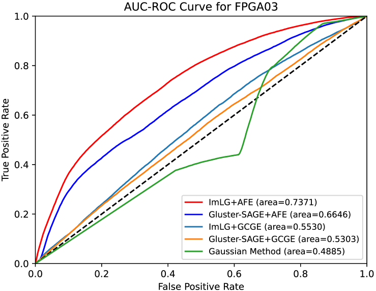
Figure 3: Performance Comparison of Various Models on FPGA03 Using AUC-ROC Curves.

V-C Comparison of feature-extraction methods

We compare the efficiency of the proposed AFE method and generalizable cross-graph embedding (GCGE) method [7] shown in TABLE III. The column headed “ImLG+AFE” indicates that the ImLG model uses the AFE method, and other columns are similar. From the statistics, the proposed AFE method consistently achieves better AUC and F1 score evaluations than the GCGE method, which indicates that the AFE method tends to generate quality features for the packing prediction task. Fig. 3 presents a performance comparison of various models on the FPGA03, indicating that graph-based approaches utilizing the AFE method outperform the Gaussian approach by a significant margin.

V-D Improvement on Physical Design

We integrate our well-trained packing predictor into our placer and present experimental results in TABLE IV. The two columns represent the placement results obtained by the placer using the Gaussian method and the ImLG model to implement the packing prediction, respectively. The“WL” and “SO” metrics indicate the routed wirelength and occupied SLICE sites, respectively. “WLR” and “SOR” represent the wirelength and occupation ratios normalized to our proposed method. The experiments show that our packing predictor improves the routed wirelength by 0.93% and SLICE occupation by 0.89%, supporting our assumption that a well-predicted model can guide the placer to achieve better wirelength with minimal resource usage.

TABLE IV: Routed Wirelength (WL) and SLICE Occupation (SO) Comparsion on ISPD 2016 Benchmarks

Methods	Our Placer[19] + Gaussian Method[4]				Our Placer[19] + ImLG
	WL	WLR	SO	SOR	WL	WLR	SO	SOR
FPGA01	322575	1.0023	8189	1.0272	321843	1.0000	7972	1.0000
FPGA02	581221	1.0044	14722	1.0035	578955	1.0000	14671	1.0000
FPGA03	2875306	1.0024	37157	1.0020	2868524	1.0000	37083	1.0000
FPGA04	4871569	1.0016	37252	1.0020	4863815	1.0000	37177	1.0000
FPGA05	9283586	1.0060	41197	1.0171	9228212	1.0000	40504	1.0000
FPGA06	5729110	1.0014	55227	1.0039	5720987	1.0000	55013	1.0000
FPGA07	8621724	1.0039	57396	1.0119	8588057	1.0000	56721	1.0000
FPGA08	7421319	1.0065	67057	1.0170	7373437	1.0000	65933	1.0000
FPGA09	10587173	1.0010	67145	1.0016	10576955	1.0000	67035	1.0000
FPGA10	6131167	1.0182	65873	1.0198	6021620	1.0000	64596	1.0000
FPGA11	10055329	1.0374	67070	1.0004	9692931	1.0000	67042	1.0000
FPGA12	6569251	1.0271	67188	1.0003	6396026	1.0000	67167	1.0000
Norm.	6087444	1.0093	48789	1.0089	6019255	1.0000	48409	1.0000

VI Conclusion

In this paper, we develop a graph learning based FPGA packing prediction framework that can achieve inductive learning on large FPGA designs with an imbalanced distribution of labels. We present dedicated feature extraction and homophily-aware feature aggregation methods to enhance node representation learning. We further propose techniques like graph oversampling and mini-batching training to tackle imbalanced label distribution in large graphs. Experimental results on the ISPD 2016 contest benchmarks showed that the proposed framework outperformed the most recent Gaussian-based method by 42.82% in F1 score. Physical design results demonstrated that our approach improved routed wirelength by 0.93% and SLICE occupation by 0.89%.

References

- [1] G. Chen, C.-W. Pui, W.-K. Chow, K.-C. Lam, J. Kuang, E. F. Y. Young and B. Yu, “RippleFPGA: Routability-driven simultaneous packing and placement for modern FPGAs,” IEEE Trans. Com-put.-Aided Design Integr. Circuits Syst., vol. 37, no. 10, pp. 2022–2035, Oct. 2017.
- [2] R. Pattison, Z. Abuowaimer, S. Areibi, G. Gréwal, and A. Vannelli, “GPlace: A congestion-aware placement tool for ultrascale FPGAs,” in Proc. ICCAD, Austin, TX, USA, 2016, pp. 1–7.
- [3] W. Li and D. Z. Pan, “A new paradigm for FPGA placement without explicit packing,” IEEE Trans. Comput.-Aided Design Integr. Circuits Syst., vol. 38, no. 11, pp. 2113–2126, Nov. 2018.
- [4] W. Li, Y. Lin and D. Z. Pan, “elfPlace: Electrostatics-based Placement for Large-Scale Heterogeneous FPGAs,” in Proc. ICCAD, Westminster, CO, USA, 2019, pp. 915–922.
- [5] W. Li, S. Dhar and D. Z. Pan, “ UTPlaceF: A routability-driven FPGA placer with physical and congestion aware packing,” IEEE Trans. Comput.-Aided Design Integr. Circuits Syst., vol. 37, no. 4, pp. 869-882, Apr. 2018.
- [6] R. Kirby, S. Godil, R. Roy, B. Catanzaro, “CongestionNet: Rout-ing congestion prediction using deep graph neural networks,” in Proc. VLSI-Soc, Cuzco, Peru, 2019, pp. 217-222.
- [7] A. Ghose, V. Zhang, Y. Zhang, D. Li, W. Liu and M. Coates, “Generalizable cross-graph embedding for GNN-based congestion prediction,” in Proc. ICCAD, Munich, Germany, 2021, pp. 1-9.
- [8] X. Chen, Z. Di, W. Wu, Q. Wu, J. Shi and Q. Feng, “Detailed routing short violation prediction using graph-based deep learning model,” in IEEE Trans. Circuits Syst. II Express Briefs, vol. 69, no. 2, pp. 564-568, Feb. 2022.
- [9] T. Zhao, X. Zhang, and S. Wang, “Graphsmote: Imbalanced node classification on graphs with graph neural networks,” in Proc. WSDM, New York, NY, USA, 2021, pp. 833–841.
- [10] W.-L. Chiang, X. Liu, S. Si, Y. Li, S. Bengio and C.-J. Hsiseh, “Cluster-GCN:An efficient algorithm for training deep and large graph convolutional networks,” in Proc. KDD, Anchorage, AK, USA, 2019, pp. 257-266.
- [11] B. Perozzi, R. AI-Rfou and S. Skiena, “Deepwalk: Online learning of social representations,” in Proc. KDD, New York, NY, USA, 2014, pp. 701-710.
- [12] J. Tang, M. Qu, M. Wang, M. Zhang, J. Yan and Q. Mei, “LINE: Large-scale information network embedding,” in Proc. WWW, Florence, Italy, 2015, pp. 1067-1077.
- [13] W. L. Hamilton, R. Ying and J. Leskovec, “Inductive representation learning on large graphs,” in Proc. NIPS, Long Beach, CA, USA, 2017, pp. 1025-1035.
- [14] K. M. Ting, “An instance-weighting method to induce cost-sensitive trees,” IEEE Trans. Knowl. Data Eng., vol. 13, no. 3, pp. 659-665, Jun. 2002.
- [15] L. Qu, H. Zhu, R. Zheng, Y. Shi and H. Yin, ”ImGAGN: Imbalanced network embedding via generative adversarial graph networks,” in Proc. KDD, Singapore, 2021, pp. 1390-1398.
- [16] N. V. Chawla, K. W. Bowyer, L. O. Hall, and W. P. Kegelmeyer, ”SMOTE: Synthetic Minority Over-sampling Technique,” J. Artif. Intell. Res., vol. 16, no.11, pp. 321-357, Mar. 2002.
- [17] H. Fan, F. Zhang, and Z. Li, “AnomalyDAE: Dual autoencoder for anomaly detection on attributed networks,” in Proc. ICASSP, Barcelona, Spain, 2020, pp. 5685-5689.
- [18] T. N. Kipf and M. Welling, “Variational graph auto-encoders,” in Proc. NIPS, 2016.
- [19] J. Mai, Y. Meng, Z. Di, and Y. Lin, “Multi-electrostatic FPGA placement considering SLICEL-SLICEM heterogeneity and clock feasibility,” in Proc. DAC, San Francisco, CA, USA, 2022, pp. 649-654.