Towards Scene-Text to Scene-Text Translation

Abstract

In this work, we study the task of “visually” translating scene text from a source language (e.g., English) to a target language (e.g., Chinese). Visual translation involves not just the recognition and translation of scene text but also the generation of the translated image that preserves visual features of the text, such as font, size, and background. There are several challenges associated with this task, such as interpolating font to unseen characters and preserving text size and the background. To address these, we introduce VTNet, a novel conditional diffusion-based method. To train the VTNet, we create a synthetic cross-lingual dataset of 600K samples of scene text images in six popular languages, including English, Hindi, Tamil, Chinese, Bengali, and German. We evaluate the performance of VTNet through extensive experiments and comparisons to related methods. Our model also surpasses the previous state-of-the-art results on the conventional scene-text editing benchmarks. Further, we present rigorous qualitative studies to understand the strengths and shortcomings of our model. Results show that our approach generalizes well to unseen words and fonts. We firmly believe our work can benefit real-world applications, such as text translation using a phone camera and translating educational materials. Code and data will be made publicly available.

1 Introduction

Machine Translation has shown remarkable growth in the last few years, partly attributed to the adoption of neural models [3, 10, 49, 8, 52, 9]. In parallel, substantial advancements have also been made in speech-to-speech translation [30, 37, 23, 31, 24] where the goal is to develop systems that are capable of accurately interpreting spoken language in one dialect and seamlessly translating it into another while preserving the voice of the original speaker, thus enabling in some cases, effective cross-lingual communication in real-time. Drawing inspiration from these research directions, we present an analogous problem in the scene text domain, namely “scene-text to scene-text translation” or, in short, “visual translation”. The visual translation task aims to translate text present in images from a source language to the target language while preserving the visual characteristics of the text and background as illustrated in Figure 1. Visual Translation has extensive applications, e.g., transforming the travel experience by allowing tourists to instantly understand sign boards in foreign languages and enabling seamless interaction with the visual world without language barriers.

Presently, understanding the text on a signboard, for instance, involves taking a picture, recognizing the text using a scene text recognizer, and then translating it using Machine Translation models. Although this process works, it is time-consuming, cognitively taxing, and becomes ineffective when seeking a seamless interaction with the visual world. Aiming to streamline this process, Google Lens [13], a popular phone application, recognizes and translates text in images and superimposes a “patch” of translated text onto the original. Although this produces a translated image, the output tends to appear unnatural, leading to poor user experience, especially when the fonts are complex, texts are curved or the background is non-uniform (We provide a case study in Section 5.6). To address this issue, our work introduces a suitable method that generates visually coherent translated text, while also generalizing to unseen fonts, text shapes, and natural scene backgrounds.

By drawing parallels with the speech-to-speech translation (S2ST) problem, we devise an approach based on widely used S2ST methods, comprising three components: automatic speech recognition (ASR), text-to-text machine translation (MT), and text-to-speech (TTS) synthesis. Similarly, we propose a visual translation system that integrates scene-text recognition (STR), text-to-text machine translation (MT), and scene-text synthesis (STS) to generate the desired image. This cascaded system offers practical advantages over an end-to-end system, as fully-supervised end-to-end training necessitates a substantial collection of input/output image pairs, which can be challenging to obtain compared to parallel text pairs for MT or image-text pairs for STR. As STR and MT models are extensively explored in the literature, and several off-the-shelf methods are available, we prioritize developing the STS model, which aims to produce the desired translated and visually coherent scene-text image while utilizing established approaches for MT and STR.

To address visual translation, we propose VTNet – a novel method that adopts a denoising diffusion probabilistic model (DDPM) based approach that aims to generate a cross-lingual text image with the supervision of a style text image in a one-shot approach. To train VTNet, a suitable cross-lingual dataset is required, which contains parallel samples of word translations. Such data should also contain similar or the same visual features for each sample, such as the font, text color, and background. However, such occurrences are rare in the wild, and thus to combat this scarcity of a parallel dataset for visual translation, we generate a synthetic dataset VT-Syn that contains 600K word-level translation samples between languages of English-to-Hindi, English-to-Tamil, English-to-Chinese, English-to-Bengali, English-to-German, and Hindi-to-English. We train our model using this synthetic dataset and evaluate its performance by translating synthetic word images as well as scene text appearing in natural scene images.

We make the following contributions:

First, we study the under-explored task of visual translation that aims to translate text in images to a target language, while preserving its font, style, position, and background. To the best of our knowledge, the comprehensive study of this problem has largely been unexplored in the existing literature.

Second, we introduce a novel conditional-diffusion-based method, VTNet to perform cross-lingual scene-text synthesis required for visual translation. It achieves the best performance on our task, surpassing the related competitive methods. Further, it also achieves state-of-the-art results on the conventional scene-text editing benchmarks.

Third, since training a visual translation model is highly infeasible using real-world images due to the unavailability of large-scale paired scene text images in two different languages, we rely on training using synthetic images. To this end, we provide a method for the synthetic generation of paired images containing words in different languages that share the same visual properties. Using this generator, we create VT-Syn, a parallel corpus of words in six languages (English, Hindi, Chinese, Bengali, Tamil, and German) containing 600K visually diverse and paired word-level translations in image form.

Fourth, we extensively evaluate our problem and model on various applications, such as the translation of text in natural images, digital images, and lecture slides. We discuss our successes and limitations associated with the problem and present directions for future research. We shall make our code and data publicly available.

2 Related Work

Machine Translation: It is a well-studied area [6, 21, 39, 10, 49, 8] that aims to convert a text from its source language to a target language. Current state-of-the-art models for machine translation are deep-learning based [10, 49, 8]. In the speech domain, Speech-to-Speech Translation (S2ST) aims to translate speech from one language to another while preserving the speaker’s voice and accent [30, 37, 23, 31, 24]. Inspired by these lines of work, we focus on text translation in the visual modality, which brings newer research challenges, such as preserving font properties and integrity of the image background, which needs to be addressed to produce visually appealing translations.

Image Generation: The generative adversarial networks (GANs) have shown impressive results for generating photo-realistic images  [12, 4, 26]. Although GANs achieve high-quality generations, they do not easily converge during training and are susceptible to mode collapse that leads to less diversity in their generations [48]. Addressing these shortcomings, a new family of likelihood-based models namely denoising diffusion  [19, 45] has emerged. They define a Markov chain of diffusion steps that gradually destruct data by adding noise and then learn to reverse the diffusion process to reconstruct the original data from noise. Unlike GANs, diffusion models have a stable training process and higher sampling diversity. They have remarkably achieved the state-of-the-art results on a wide array of generation tasks such as text-to-image generation [42, 43], audio generation [28], 3D-shape generation [38], and video generation [18]. We adopt them for our task, and to the best of our knowledge, we are the first to introduce a diffusion-based model in the area of scene-text editing.

Editing Text in Images: The problem of editing text in images has witnessed significant research interest in recent years [50, 51, 41, 32, 29, 40]. This task aims to modify scene text to target content while retaining visual properties of the original text. SRNet [50] is one such method that learns an end-to-end GAN-based style-retention network. SwapText [51] improved upon the SRNet architecture by modeling the geometrical transformation of the text using spatial points. More recently, TextStyleBrush [29], RewriteNet [32], and MOSTEL [40] introduce a self-supervised training approach on real-world images for this task. Further, TextStyleBrush is evaluated on handwritten images as well. Authors in [41] proposed a character-wise text editor model for this task. However, their approach assumes source and target text instances are of the same length, which is not always true, especially in the translation task. A more recent approach MOSTEL [40] also introduces stroke-level modifications to produce more photo-realistic generations. Despite demonstrating a few selected qualitative results for cross-lingual editing, these works have only scratched the surface of this area and it remains largely unexplored and understudied. Our work aims to fill this gap.

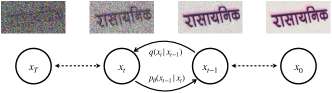
Figure 2: Overview of the diffusion process: (i) forward process $q$ corrupts the image $x_{0}$ through iterative addition of noise, and (ii) reverse process $p_{\theta}$ reconstructs the original image by predicting the noise added at each timestep $t$.

3 Background on Diffusion Model

In this section, we briefly review the denoising diffusion probabilistic model (DDPM) [19, 45] or diffusion model, which has demonstrated impressive performance in the task of image generation [7, 42, 43, 5]. Diffusion models are generative models that gradually introduce noise to data and use a probabilistic approach to reverse this process and learn the underlying data distribution. The model employs Markov chains to perform two steps: (i) the forward or diffusion process that corrupts the input data $x_{0}$ through iterative addition of noise, and (ii) the reverse or denoising process that learns to recover the original data $x_{0}$ by denoising the latent variable $x_{T}$, where $T$ is the total number of diffusion steps. The model assumes $x_{t}\in\mathbb{R}^{d}$ to be the result at the end of each diffusion timestep $t\in\{1,2,\ldots,T\}$, with all sharing the same dimension of $d$. The forward process is deterministic, whereas the reverse process is parameterized by a learnable neural network. Figure 2 illustrates the diffusion model, and the supplementary material provides a formal description of both processes.

4 VTNet: A Diffusion-based Visual Translation Network

Given an image of a word in the source language ($x_{src}$), our goal is to generate an image of the word in the target language ($x_{tgt})$, i.e., perform scene text-to-scene text translation. To this end, we introduce Visual Translation Network (VTNet) – a unified framework that involves a two-stage generation process as illustrated in Figure 3 (a). VTNet is a conditional diffusion-based model that is trained to generate three images in the visual translation process – the background, foreground, and target images. Formally, given the source image $x_{src}$ and a gray-scale target word image $x_{w}$, we aim to learn a conditional noise predictor $f_{\theta_{1}}$ to generate the background $x_{bg}$ and foreground images $x_{fg}$. Further, we utilize $x_{bg}$ and $x_{fg}$ to learn a conditional noise predictor $f_{\theta_{2}}$ for the generation of the target image $x_{tgt}$. Table 1 describes the major notations used in this paper. We describe VTNet and its training and inference below.

Notation	Description
$T$	Total number of time steps in the diffusion process
$x_{t}$	Image at time step $t$
$x_{src}$	Image of word in source language
$x_{tgt}$	Image of word in target language
$x_{w}$	Gray-scale image of target word
$x_{bg}$	Image of text-free background
$x_{fg}$	Image of source text as foreground
$\eta_{t}$	Noise sampled from Gaussian $\mathcal{N}$ at time $t$
$t_{e}$	Embedding for time step $t$
$\beta_{t}$	Variance schedule for the diffusion process
$f_{\theta_{1}},f_{\theta_{2}}$	Parameterized conditional noise predictor networks
$E_{src},E_{w},E_{fb}$	Parameterized image encoder networks

Table 1: Notations used in this paper.

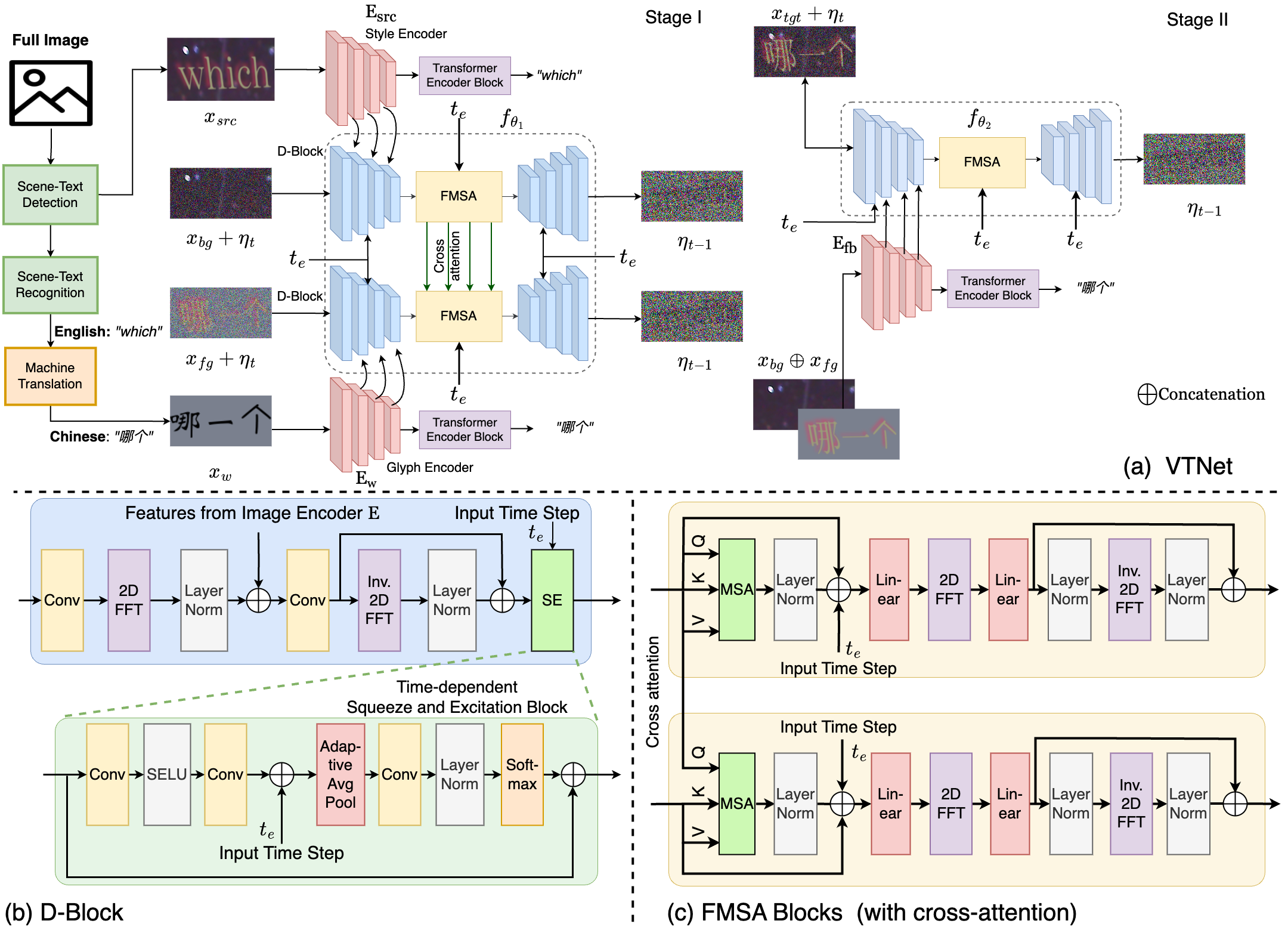
Figure 3: Our method, VTNet involves cross-lingual editing of text in a source image ($x_{src}$) to generate the target image ($x_{tgt}$) while preserving the visual properties of the text. (a) Training of VTNet is in two stages: (i) Stage I involves learning a noise predictor network ($f_{\theta_{1}}$) for background ($x_{bg}$) and foreground images ($x_{fg}$), that is conditioned on the source ($x_{src}$) and target word ($x_{w}$) images respectively; (ii) Stage II involves learning a noise predictor network ($f_{\theta_{2}}$) for $x_{tgt}$, that is conditioned on the concatenated input of $x_{fg}\oplus x_{bg}$. (b) Overview of the Decoder Block (D-Block) and its components. (c) Overview of the Fourier-based Multiheaded Self-Attention (FMSA) block. (SE: Squeeze-and-Excitation block [20], SELU: Scaled Exponential Linear Unit, MSA: Multiheaded Self-Attention, FFT: Fast-Fourier Transform).

Conditional Noise Predictor Network: The conditional noise predictor network $f_{\theta}$ predicts the noise $\eta_{t}$ added at each timestep in the diffusion process and is conditioned on input image information. As illustrated in Figure 3 (a), VTNet consists of two noise predictors $f_{\theta_{1}}$ and $f_{\theta_{2}}$. Each of them takes a word image $x_{t}$, output of the image encoder $E$, and timestep embedding $t_{e}$ as input. It consists of four D-blocks for down-sampling (Figure 3 (b)), followed by eight FMSA blocks (Figure 3 (c), and four additional D-blocks to perform upsampling of the feature maps. The D-Block consists of a sequence of convolution, Fast Fourier Transform (FFT), inverse Fast Fourier Transform (inverse FFT), and an adaptation of the Squeeze and Excitation (SE) block [20] which is dependent on timestep information. Our utilization of Fourier-convolutions is motivated by their recent success in generative tasks of image inpainting [47] and image super-resolution [44] which improves perceptual quality and parameter efficiency of the network. The SE block is utilized to selectively emphasize informative features and suppress less informative ones, resulting in improved performance. The FMSA block consists of a multiheaded-self attention layer (MSA) [49] followed by linear and Fourier operations. In the noise predictor $f_{\theta_{1}}$, we perform cross-attention between the FMSA blocks, inspired by the co-attention mechanism in ViLBERT [35] to facilitate information transfer from source image $x_{src}$ to generate foreground image $x_{fg}$.

Training: Image Encoder: An image encoder $E$ encodes information from input images, which is added to each downsampling D-Block in the noise predictor network to conditionally guide the generation process. In VTNet, we use three image encoders: (i) Style Encoder $E_{src}$ for encoding style of the source image, (ii) Glyph Encoder $E_{w}$ for encoding the glyphs and characters of the target text content, and (iii) Target Image Encoder $E_{fb}$ for encoding the generated foreground and background content, as shown in Figure 3 (a). It utilises four D-Block networks as employed in the noise predictor network. Each image encoder is also appended with two transformer encoder blocks that are used to train the model using CTC loss [15], to better encode the text content in images. As shown in Figure 3 (a), training is performed in the following two stages: In the stage-1, we aim to a learn conditional noise predictor to generate $x_{bg}$ and $x_{fg}$ conditioned on the $x_{src}$ and $x_{w}$ image input, respectively. Let $T$ be the total diffusion steps, $E_{src}$ and $E_{w}$ be the image encoders, and $f_{\theta_{1}}$ be the conditional noise predictor at stage I. We encode $x_{src}$ and $x_{w}$ as follows: $x_{{src}_{e}}=E_{src}(x_{src})$ and $x_{w_{e}}=E_{w}(x_{w})$. We then sample noise $\eta_{t}\sim\mathcal{N}(\mathbf{0},\mathbf{I})$ at timestep $t\sim\{0,1,\ldots,T-1\}$. Further, we optimize the noise predictor in Stage I by taking the gradient step on:

$$\nabla_{\theta}||\eta_{t}-f_{\theta_{1}}(x_{{fg}_{r}},x_{{bg}_{r}},x_{{src}_{e}},x_{w_{e}},t)||,$$ (1)

where,

$$x_{{fg}_{r}} = \sqrt{\bar{\alpha}_{t}}x_{fg}+\sqrt{1-\bar{\alpha}_{t}}\eta_{t},$$ (2)

$$x_{{bg}_{r}} = \sqrt{\bar{\alpha}_{t}}x_{bg}+\sqrt{1-\bar{\alpha}_{t}}\eta_{t}.$$ (3)

by setting $\alpha_{t}=1-\beta_{t}$ and $\bar{\alpha_{t}}=\prod_{s=1}^{t}\alpha_{s}$ where $\beta_{t}$ is the variance schedule of the diffusion process that determines how much noise is added at each timestep.

In the stage-2, we consider $E_{fb}$ as the image encoder for the target image $x_{tgt}$, which is conditioned on the concatenation of the generated background and foreground images $(x_{fg}\oplus x_{bg})$. We consider $T$ as the total diffusion steps and $f_{\theta_{2}}$ as the conditional noise predictor. We encode $(x_{fg}\oplus x_{bg})$ as $x_{fb_{e}}=E_{fb}(x_{fg}\oplus x_{bg})$. Then we sample noise $\eta_{t}\sim\mathcal{N}(\mathbf{0},\mathbf{I})$ and timestep $t\sim\{0,1,\ldots,T-1\}$. Further, we optimize the noise predictor in this Stage by taking the gradient step on:

$$\nabla_{\theta}||\eta_{t}-f_{\theta_{2}}(x_{{tgt}_{r}},x_{fb_{e}},t)||$$ (4)

where,

$$x_{{tgt}_{r}}=\sqrt{\bar{\alpha}_{t}}x_{tgt}+\sqrt{1-\bar{\alpha}_{t}}\eta_{t}.$$ (5)

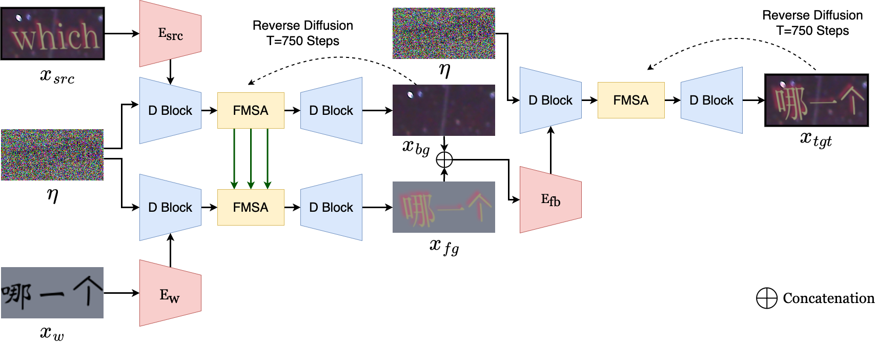
Figure 4: Model Inference. During model inference, given a source image $x_{src}$ and synthetically-generated target word image $x_{w}$, we use the learned conditional noise predictor $f_{\theta_{1}}$ to generate the background $x_{bg}$ and foreground $x_{fg}$ images from sampled noise $\eta$. The generations are then used by $f_{\theta_{2}}$ to generate the target image $x_{tgt}$ in the desired language. This generation occurs through a reverse diffusion process over $T$=750 steps.

Inference. In the inference stage, we use the learned VTNet to generate the target image $x_{tgt}$ from sampled Gaussian noise $\eta_{T}$, conditioned source image $x_{src}$, target word image $x_{w}$ inputs as illustrated in Figure 4. Similar to training, we perform inference in two stages: (i)In the first stage, we are given the source image $x_{src}$ and target word image $x_{w}$, learned conditional noise predictor $f_{\theta_{1}}$ and image encoders $E_{src}$ and $E_{w}$ and we consider $T$ steps for the reverse diffusion process. We sample noise $\eta_{t}\sim\mathcal{N}(\mathbf{0},\mathbf{I})$ and encode $x_{src}$ and $x_{w}$ as $x_{{src}_{e}}=E_{src}(x_{src})$ and $x_{{w}_{e}}=E_{w}(x_{w})$. Starting from timestep $t=T-1$ to $t=0$ we re-compute $\eta_{t-1}$ as follows:

$$\eta_{t-1}=\frac{1}{\sqrt{\bar{\alpha_{t}}}}\left(\eta_{t}-\frac{1-\alpha_{t}}{\sqrt{(1-\bar{\alpha_{t}})}}f_{\theta_{1}}(\eta_{t},\eta_{t},x_{{src}_{e}},x_{w_{e}},t)\right).$$ (6)

These steps are repeated in reverse progression until $t=0$ step where we obtain $x_{fg}$ and $x_{bg}$ images. (ii) In syage-2, we utilize the concatenation of $x_{fg}$ and $x_{bg}$ images to conditionally generate the target image $x_{tgt}$. We consider the learned image encoder $E_{fb}$ and conditional noise predictor $f_{\theta_{2}}$, and $T$ steps for the reverse diffusion process. We sample noise $\eta_{t}\sim\mathcal{N}(\mathbf{0},\mathbf{I})$ and obtain $x_{fb_{e}}=E_{fb}(x_{fg}\oplus x_{bg})$. Starting from timestep $t=T-1$ to $t=0$ we re-compute $\eta_{t-1}$ as follows:

$$\eta_{t-1}=\frac{1}{\sqrt{\bar{\alpha_{t}}}}\left(\eta_{t}-\frac{1-\alpha_{t}}{\sqrt{(1-\bar{\alpha_{t}})}}f_{\theta_{2}}(\eta_{t},x_{{fb}_{e}},t)\right).$$ (7)

At the end of this reverse diffusion, we obtain the final target word image $x_{tgt}$ in desired language.

Method	Eng $\rightarrow$ Hin			Eng $\rightarrow$ Tam			Eng $\rightarrow$ Ben
	P $\uparrow$	S $\uparrow$	F $\downarrow$	P $\uparrow$	S $\uparrow$	F $\downarrow$	P $\uparrow$	S $\uparrow$	F $\downarrow$
SRNet [50]	23.04	0.840	28.08	23.98	0.839	28.80	25.88	0.831	27.99
SwapText [51]	27.09	0.881	24.76	26.87	0.880	22.19	27.98	0.862	24.52
MOSTEL [40]	30.87	0.910	15.21	31.09	0.910	14.67	29.98	0.910	15.00
VTNet (Ours)	34.98	0.930	10.09	35.78	0.950	10.19	34.02	0.932	11.52
Method	Eng $\rightarrow$ Chi			Eng $\rightarrow$ Ger			Hin $\rightarrow$ Eng
	P $\uparrow$	S $\uparrow$	F $\downarrow$	P $\uparrow$	S $\uparrow$	F $\downarrow$	P $\uparrow$	S $\uparrow$	F $\downarrow$
SRNet [50]	26.00	0.840	29.90	26.19	0.851	28.02	24.31	0.840	29.01
SwapText [51]	26.99	0.871	25.98	28.34	0.881	22.01	26.78	0.870	24.10
MOSTEL [40]	30.12	0.908	14.02	29.92	0.910	15.08	28.78	0.910	13.96
VTNet (Ours)	35.19	0.951	12.07	35.02	0.953	9.01	32.00	0.949	10.54

Table 2: Performance comparison across baselines on the VT-Syn test set. Details in Section 5.4 (P: PSNR, S: SSIM, F: FID, Eng: English, Hin: Hindi, Tam: Tamil, Ben: Bengali, Chi: Chinese, Ger: German).

5 Experiments

5.1 Datasets

VT-Syn. To study visual translation, a dataset is required which contains paired images of text in different languages with identical visual properties (style, font, orientation, and size). However, obtaining such data from the real world is impractical due to the rarity of visually identical translated texts. To overcome this challenge, we introduce VT-Syn, a synthetically generated corpus of 600K visually diverse translated word images in six languages: English, Hindi, Chinese, Bengali, Tamil, and German. We utilized an Indic-language scene-text image generator [36] and modified it to generate samples of scene-text in paired languages with controllable parameters for font, style, color, and spatial transformations to ensure visual diversity. Each sample contains source image ($x_{src}$), target word image ($x_{w}$), background image ($x_{bg}$), foreground image ($x_{fg}$), and target image ($x_{tgt}$). We collect 560 publicly available fonts and use a vocabulary of 3K commonly used words in each target language and use [14] to get the corresponding translations in source language. Few samples from VT-Syn are shown in Figure 5. Train-Test Split: The dataset is divided into six categories of translations: (i) English $\rightarrow$ Hindi, (ii) English $\rightarrow$ Chinese, (iii) English $\rightarrow$ Bengali, (iv) English $\rightarrow$ Tamil, (v) English $\rightarrow$ German, and (vi) Hindi $\rightarrow$ English, each set containing 100K samples. We use 85K, 10K, and 5K samples chosen at random for the train, test and validation set, respectively. Data and generation code will be made publicly available. More details provided in the supplementary material.

ICDAR 2013 [25] was created as part of the ICDAR Robust Reading Competition [25]. It consists of 1.1K natural scene-text images that primarily feature English words. Despite not including paired images of translated words, we use this dataset to evaluate the performance of the baselines on real-world images using text recognition accuracy as an indirect metric.

IIIT-ILST [36] consists of 3K multilingual natural scene-text images, and was proposed to evaluate scene-text recognition methods in Indic languages [36]. We use a subset of this dataset containing Hindi words to evaluate Hin$\to$Eng baselines.

Temper-Syn2k and Temper-Scene [40] are evaluation datasets for the conventional scene-text editing task. Temper-Syn2k contains 2K synthetically created English word pairs, and Temper-Scene contains 7.7K real scene-text source images. We evaluate VTNet on this data to understand its performance in the conventional English-to-English scene-text editing task.

Additionally, we also create 25 digital-born images of internet memes and lecture slides to qualitatively analyze the performance of our model on digital images in Section 8.

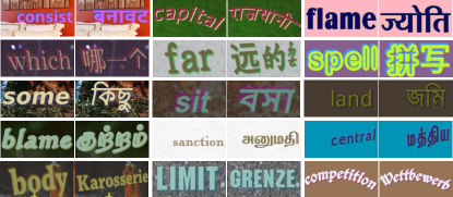
Figure 5: VT-Syn dataset examples, which contains synthetically generated images of translated words in different languages with diverse fonts, text colors, sizes, orientations, and backgrounds (natural scene, texture or plain colors).

5.2 Baselines

We compare our VTNet with three competitive scene-text editing approaches: (i) SRNet [50], which is a modular generative method that uses a GAN architecture and a pre-trained VGG19 model. As the original implementation is not publicly available, we use a third-party implementation; (ii) SwapText [51] extends the SRNet architecture by adding a text-swapping network and a self-attention network to learn better correspondences between the content and style features; and (iii) MOSTEL [40] is the state-of-the-art scene-text-editing baseline, which introduces a framework for stroke-level modifications that prioritize learning editing rules in text regions and preserve the integrity of background regions. All methods are trained in a supervised setting on the VT-Syn train sets to ensure a fair comparison. Note that other scene-text editing models, such as RewriteNet [32] and TextStyleBrush [29], did not have publicly available implementations when writing this paper.

Method	E$\to$H	E$\to$T	E$\to$B	E$\to$C	E$\to$G	H$\to$E
SRNet [50]	0.39	0.43	0.40	0.42	0.41	0.48
SwapText [51]	0.54	0.57	0.59	0.57	0.56	0.55
MOSTEL [40]	0.80	0.75	0.74	0.70	0.84	0.87
VTNet (Ours)	0.83	0.77	0.77	0.72	0.87	0.89
Ground Truth	0.85	0.77	0.77	0.75	0.88	0.91

Table 3: Text recognition accuracy on visually translated images from the VT-Syn test set. The column source $\rightarrow$ target indicates that the recognizer is evaluated on the target language. Results on Ground Truth (original target) images are also provided for reference. (E: English, H: Hindi, T: Tamil, B: Bengali, C: Chinese, G: German).

Method	ICDAR 2013 [25]				IIIT-ILST [36]
	E$\to$H	E$\to$T	E$\to$B	E$\to$C	H$\to$E
SRNet [50]	0.39	0.30	0.32	0.41	0.48
SwapText [51]	0.41	0.30	0.34	0.43	0.48
MOSTEL [40]	0.45	0.32	0.36	0.46	0.50
VTNet (Ours)	0.46	0.34	0.38	0.48	0.52

Table 4: Text recognition accuracy on visually translated images from datasets containing real-world images.

5.3 Evaluation Metrics

We use standard evaluation metrics that are commonly used in the scene-text editing [50, 51, 29] and image generation [17] literature to evaluate the performance of baselines on the Visual Translation task: (i) PSNR, which is the peak signal-to-noise ratio, (ii) SSIM, which is the mean of structural similarity and (iii) Fréchet inception distance or FID, which is the distance between features extracted by pre-trained InceptionV3 [17]. We aim for higher PSNR and SSIM values and lower FID values. Additionally, we evaluate the readability of the generated text using a scene-text recognizer [2] in the target language, and report the text recognition accuracy, as done in [29, 40]. To measure the subjective quality of image generation, we also conduct a human evaluation study to assess the relative preference between the baseline generations in Section 5.7.

Method	Temper-Syn2k [40]				Temper-Scene [40]
	MSE$\downarrow$	PSNR$\uparrow$	SSIM$\uparrow$	FID$\downarrow$	Acc$\uparrow$
pix2pix [22]	0.0732	12.01	0.349	164.24	18.382
SRNet [50]	0.0193	18.66	0.610	41.26	32.298
SwapText [51]	0.0174	19.43	0.652	35.62	60.634
MOSTEL [40]	0.0123	20.81	0.721	29.48	76.790
VTNet (Ours)	0.0083	23.36	0.740	26.29	79.890

Table 5: Quantitative results on the conventional scene-text editing task, evaluated on the Temper-Syn2k and Temper-Scene datasets [40].

Method	PSNR$\uparrow$	SSIM$\uparrow$
w/o Cross-attention layer	27.98	0.899
w/o Fourier-Conv layers	29.99	0.919
w/o SE Blocks	30.92	0.901
w/o FMSA Blocks	25.63	0.857
w/o Text Recognition	33.91	0.939
VTNet (Full Model)	34.50	0.944

Table 6: Ablation study results comparing the performance of the proposed VTNet with specific components removed on VT-Syn test set (w/o: ”without”).

Method	PSNR$\uparrow$	SSIM$\uparrow$
VAE [27]	25.08	0.844
Pix2Pix [22]	28.72	0.882
WGAN [1]	30.90	0.910
WGAN-GP [16]	31.21	0.925
Ours	34.50	0.944

Table 7: Performance comparison of VTNet with various generative model architectures on VT-Syn test set.

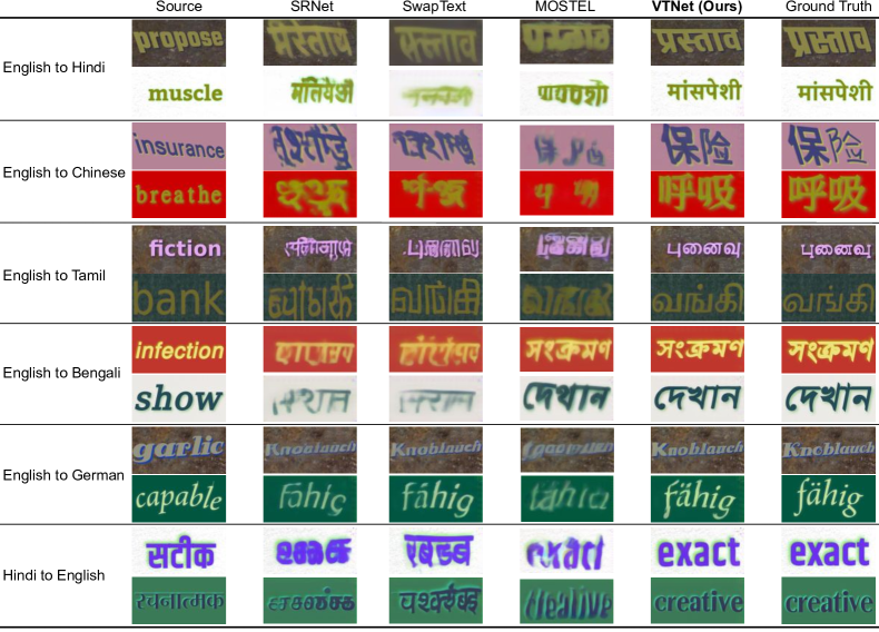
Figure 6: Word-level Results. We show a few generation results from the baselines on the VT-Syn test set. We also provide source and ground truth target images for reference (best viewed in color).

5.4 Results and Discussions

Main Results: We present the results of our visual translation task on the VT-Syn test set in Table 2. We trained each baseline for every translation category in the dataset. Our proposed model, VTNet, outperforms all baseline methods across all categories and metrics. We noticed that GAN-based models such as SRNet, SwapText, and MOSTEL underperformed our diffusion-based generative model. We believe this is due to the well-known issue of lower diversity in generations by GAN-based models and their tendency for mode collapse. While MOSTEL outperformed SRNet and SwapText by following stroke guidance maps to identify explicit text regions to edit, it still failed to surpass the superior generational quality of our VTNet, as shown in Figure 6.

Text Recognition Accuracy: In addition to measuring the visual appearance of the generations using PSNR, SSIM, and FID, we also measured the correctness and legibility of the generated text through the text recognition accuracy metric. We used ViTSTR [2] scene-text recognizer (pre-trained on each target language) in Table 3 for synthetic images on the VT-Syn test set, and Table 4 for real-world images from the ICDAR’13 [25] and IIIT-ILST [36] datasets. Although this is the only indirect metric to assess performance on real-world images, it does not account for consistency in visual properties, which is important for our task.

Scene-Text Editing: To evaluate how well VTNet performs on conventional and well-explored scene-text editing task, we tested it on two standard public benchmarks: Temper-Syn2k and Temper-Scene [40]. Our method outperformed the previous state-of-the-art baseline, MOSTEL, on every metric in both benchmarks, as shown in Table 5. These results confirm the superiority of diffusion-based models in general scene-text editing tasks.

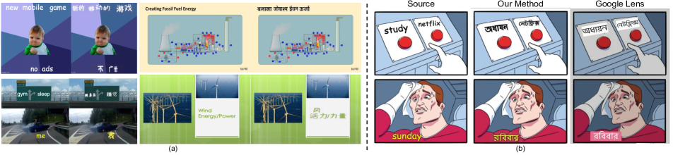
Figure 7: Visual translation results for digital-born images of memes and lecture slides. In (b) we compare VTNet with Google Lens, a popular phone app, that does not interpolate fonts or maintain background consistency in the visual translation task.

Metric	Total Diffusion Steps
	150	250	350	500	750	1000
PSNR $\uparrow$	27.9	29.3	30.4	31.9	33.9	34.5
SSIM $\uparrow$	0.87	0.88	0.90	0.91	0.93	0.94
Time (s)	3.00	4.00	4.81	5.9	8.81	10.10

Table 8: Analysis of VTNet with respect to the number of total diffusion steps ($T$). Time indicates inference time.

Method	PSNR $\uparrow$	SSIM $\uparrow$	Size (M params)	Time (s)
Small	28.52	0.868	3.36	3.90
Medium	30.78	0.891	4.21	4.87
Large	32.76	0.928	5.49	6.78
X-Large (Ours)	34.50	0.944	8.20	8.76

Table 9: Model-size based analysis for VTNet. Model sizes are varied by adjusting the number of blocks in the FMSA component (Small: 1, Medium: 3, Large: 6, and X-Large: 8 blocks). Size indicates model size measured in million parameters.

Method	Steps	P $\uparrow$	S $\uparrow$	F $\downarrow$	Time (s)
SRNet [50]	-	24.90	0.840	28.60	0.88
SwapText [51]	-	27.33	0.876	23.90	0.90
Mostel [40]	-	30.12	0.909	14.65	0.83
VTNet	750	34.50	0.944	10.57	8.76
VTNet (DDIM [46])	10	34.01	0.939	11.21	1.82
VTNet (DPM-Solver++ [34])	6	34.12	0.940	11.04	0.89

Table 10: Impact of Diffusion Samplers (DDIM and DPM-Solver++) on VTNet with a comparison to other baselines. Steps refer to total diffusion steps.

5.5 Ablation and Analysis

Ablation Study: We conducted an ablation study on our VTNet model to understand the contribution of each component. We evaluated the impact of removing the cross-attention layer between the Fourier-based Multiheaded Self-Attention (FMSA) blocks by replacing it with a simple D-block connection. We also removed specific layers in the D-blocks and FMSA blocks such as the Fourier-Convolutional (FC) layers, Squeeze-and-Excitation (SE) blocks, and the FMSA blocks themselves. Furthermore, we measured the importance of the text-recognition objective in our network. The results, presented in Table 6, show that removing any of these components leads to a degradation in performance across all metrics compared to the full VTNet model. Notably, the cross-attention layer is the most crucial component, while using FC and SE blocks leads to further improvements.

Effect of generative model backbones: We compared the performance of VTNet with various generative model backbones, including VAE [27], Pix2Pix [22], WGAN [1], and WGAN-GP [16], as shown in Table 7. As expected, using diffusion leads to improved quality in our task over GAN-based methods. Among the GAN-based methods, WGAN-GP performs closest to our method.

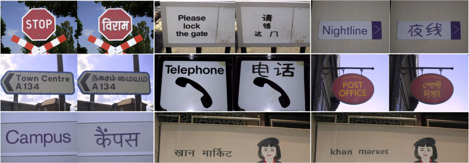
Figure 8: A selection of visual translation results for natural scene images shown in pairs (Left: source, Right: translated). These results are verified and found correct by native speakers of these languages.

Effect of diffusion steps: We varied the number of diffusion steps $T$ and evaluated the performance of VTNet on our task. Results are shown in Table 8. Increasing $T$ leads to higher PSNR and SSIM values but also longer inference time. However, the performance improvement becomes marginal after $T=750$, while inference time significantly increases. Therefore, we chose $T=750$ as the optimal hyperparameter value.

Model size: We evaluated the impact of model size on performance by varying the number of FMSA-Blocks in VTNet and reported the results in Table 9. As we increased the number of FMSA-Blocks, the performance consistently improved, indicating that our diffusion model benefits from a more capable and parameterized network.

Usage of Diffusion Samplers: In order to enable real-time inference for visual translation, we optimized our VTNet using diffusion samplers. These samplers are advanced solvers for diffusion models, significantly reducing the required time-steps (around 10) while maintaining high generation quality. We evaluated two samplers, DDIM [46] and DPM-Solver++[34], as shown in Table10. The results show that using a sampler such as DPM-Solver++ achieves a remarkable 10$\times$ reduction in inference time with just 6 time-steps, causing only a marginal decrease in performance. This demonstrates the potential of such efficient samplers for real-world applications, particularly for “instant” visual translation using mobile phone cameras.

5.6 Qualitative Analysis

To evaluate the effectiveness of our method, we conduct a qualitative analysis on natural scene images. We detect text in the images using EAST [53] and recognize the text using ViTSTR [2]. Our VTNet model is then applied to obtain the visual translation results. Figure8 presents the visual translation process for scene-text in natural images selected from the ICDAR 2003[25] and IIIT-ILST [36] datasets. Our model captures various text styles and fonts commonly seen in the real world and can generalize to different languages. In addition, we present qualitative results for visual translation in digitally-created images of internet memes and educational lecture slides in Figure7(a). Further, we compare the visual translation results between our method and Google Lens, a popular mobile phone app in Figure 7(b). At the time of writing this paper, although Google Lens can perform correct translations, it fails to accurately match the visual properties of the source text, resulting in translations that may appear unnatural and not photo-realistic.

Method	Hin$\to$Eng	Eng$\to$Hin	Eng$\to$Tam	Eng$\to$Ben
SRNet [50]	2.0	4.0	8.0	8.0
SwapText [51]	8.0	10.0	10.0	12.0
MOSTEL [40]	16.0	18.0	8.0	16.0
VTNet (Ours)	74.0	70.0	68.0	64.0

Table 11: Human evaluation of generated results, expressed as relative percentage preferences between generations produced by the baselines. Details in Section 5.7.

5.7 Human Evaluation

Evaluating text style and appearance is often subjective. To compare generations by baselines, we conduct a human evaluation. We assess preferences for generations produced by baseline models across four language translations: Eng$\rightarrow$Hin, Hin$\rightarrow$Eng, Eng$\rightarrow$Ben, and Eng$\rightarrow$Tam. We randomly select 25 real-world examples from ICDAR 2013 [25] and IIIT-ILST [36], and 25 synthetic examples from VT-Syn test set. We then present each evaluator with image generations in their native language from each baseline and ask them to choose their preferred generation based on text appearance and correctness. Four native speakers of the target languages, aged between 21-28, participate in the study. The results of our evaluation are presented in Table 11. We find that evaluators predominantly prefer the generations from our model across all four languages over that of SRNet [50], SwapText [51], and MOSTEL [40]. We attribute this preference to the superior generation quality achieved by our diffusion-based generative model.

5.8 Implementation Details

Xavier initialization [11] is used to initialize the 8.2M parameters of VTNet. It is trained end-to-end with a batch size of 64 for 800K iterations, with input sizes varying between 128$\times$64 and 256$\times$128 to handle image size variability. The AdamW [33] optimizer with an initial learning rate of $1e-5$ and exponential weight decay is used to optimize the training of the Stage 1 network, while RMSProp optimizer with a learning rate of $1e-4$ and a linear scheduler is used for the Stage 2 network. Both networks are trained for 50 hours on 2$\times$ Nvidia A5000 GPUs with 24GB VRAM each. More details are provided in the supplementary paper.

6 Limitations and Future Work

While our proposed framework has demonstrated promising results through extensive quantitative, qualitative, and human evaluations, there are still some limitations to address: (i) Single-Word Translation: Currently, our framework can only perform single-word generation and is not trained for phrase-level or sentence-level translation. (ii) Inference Time: VTNet takes approximately 0.89 seconds to generate when using DPM-Solver++, which needs to be further optimized for real-time applications. (iii) Font Coverage: Our model supports translations among only six different languages and 560 different text fonts. We leave addressing these challenges as a future scope of this work.

7 Conclusion

We presented VTNet – a diffusion-based model for the under-explored yet important task of visual translation of scene text. Our model currently supports translation between English to Hindi, English to Tamil, English to Bengali, English to Chinese, English to German, and Hindi to English languages. We conduct extensive experiments and ablations that demonstrate the efficacy and superiority of our proposed diffusion-based approach. We also qualitatively analyze our results that further highlight the application of our work for visual translation in the domains of natural scene-text images, digital memes, and lecture slides. In the future, we aim to increase our coverage of fonts and languages and move from word-level to line-level translation.

Appendix A Diffusion Processes

Here we provide a formal description of the forward and reverse diffusion processes involved in Diffusion Models [19].

Forward Process. The posterior $q(x_{1:T}|x_{0})$ is termed as the diffusion or forward process. This process transforms the input data $x_{0}\sim q(x_{0})$ to pure noise $x_{T}\sim q(x_{T})$. The forward process is fixed to a Markov chain which iteratively generates a sequence $x_{1},x_{2},\ldots,x_{T}$ by adding Gaussian noise $\eta$ to the data according to a noise schedule $\{\beta_{t}\in(0,1)\}_{t=1}^{T}$. We express this mathematically below:

$$\begin{split}q(x_{1:T}|x_{0})=\prod_{t=1}^{T}q(x_{t}|x_{t-1}),\\ q(x_{t}|x_{t-1})=\mathcal{N}(x_{t};\sqrt{1-\beta_{t}}x_{t-1},\beta_{t}\mathbf{I}),\end{split}$$ (8)

Here $\mathcal{N}$ is a Gaussian distribution, $\beta_{t}$ is a constant, and $\mathbf{I}$ is an identity covariance matrix. By setting $\alpha_{t}=1-\beta_{t}$ and $\bar{\alpha_{t}}=\prod_{s=1}^{t}\alpha_{s}$, we can sample $x_{t}$ at any timestep $t$ in closed form:

$$q(x_{t}|x_{0})=\mathcal{N}(x_{t};\sqrt{\bar{\alpha_{t}}}x_{0},(1-\bar{\alpha_{t}})\mathbf{I}),$$ (9)

This can be further reparameterized as:

$$x_{t}=\sqrt{\bar{\alpha_{t}}}x_{0}+\sqrt{1-\bar{\alpha_{t}}}\eta,\quad\eta\sim\mathcal{N}(\mathbf{0},\mathbf{I}).$$ (10)

Reverse Process. The reverse process seeks to regenerate the input data $x_{0}$ from the Gaussian noise $x_{T}$. This process is linked to a Markov chain parameterized with a prior distribution $p(x_{T})=\mathcal{N}(x_{T};\mathbf{0},\mathbf{I})$ and a learnable transition kernel $p_{\theta}(x_{t-1}|x_{t})$:

$$\begin{split}p_{\theta}(x_{0:T-1}|x_{T})=\prod_{t=1}^{T}p_{\theta}(x_{t-1}|x_{t}),\\ p_{\theta}(x_{t-1}|x_{t})=\mathcal{N}(x_{t-1};\mu_{\theta}(x_{t},t),\rho_{\theta}(x_{t},t)^{2}\mathbf{I}),\end{split}$$ (11)

Here $\mu_{\theta}$ and $\rho_{\theta}$ represent the learnable mean and variance functions, respectively. However, following [19], we keep the variance fixed to $\mathbf{I}$ and only learn the mean $\mu_{\theta}$.

During training, we maximize the variational lower bound (ELBO) on negative log-likelihood and use KL-divergence and variance reduction [19]:

$$\mathbb{E}[-\log p_{\theta}(x_{0})]\leq L=\mathbb{E}_{q}\bigg{[}\underbrace{D_{KL}({q(x_{T}|x_{0})}~{}||~{}{p(x_{T})}}_{L_{T}})$$

$$+\sum_{t>1}\underbrace{D_{KL}({q(x_{t-1}|x_{t},x_{0})}~{}||~{}{p_{\theta}(x_{t-1}|x_{t}))}}_{L_{t-1}}\underbrace{-\log p_{\theta}(x_{0}|x_{1})}_{L_{0}}\bigg{]}.$$ (12)

This transformation requires a direct comparison between $p_{\theta}(x_{t-1}|x_{t})$ and its corresponding diffusion process posteriors. Setting $\tilde{\mu}_{t}(x_{t},x_{0})=\frac{\sqrt{\bar{\alpha}_{t-1}}\beta_{t}}{1-\bar{\alpha}_{t}}x_{0}+\frac{\sqrt{\alpha_{t}}(1-\bar{\alpha}_{t-1})}{1-\bar{\alpha}_{t}}x_{t}$, we have

$$q(x_{t-1}|x_{t},x_{0})=\mathcal{N}(x_{t-1};\tilde{\mu}_{t}(x_{t},x_{0}),\tilde{\beta}_{t}\textbf{I}).$$ (13)

Eq. (9), (11) and (13) assure that all KL divergences in Eq. (12) are comparisons between Gaussians. With $\sigma_{\theta}^{2}=\tilde{\beta}_{t}=\frac{1-\bar{\alpha}_{t-1}}{1-\bar{\alpha}_{t}}\beta_{t}$ for $t>1,~{}\tilde{\beta}_{1}=\beta_{1}$, and constant $C$, we have

$$L_{t-1}=q{\frac{1}{2\sigma_{t}^{2}}\|\tilde{\mu}_{t}(x_{t},x_{0})-\mu_{\theta}(x_{t},t)\|^{2}}+C.$$

The training process follows [19], where the evidence lower bound (ELBO) is simplified, with $x_{0}$ and $t$ as inputs with $f_{\theta}$ as the learnable noise predictor:

$$\min_{\theta}L_{t-1}(\theta)=\mathbb{E}_{x_{0},\eta,t}\Bigr{[}{\|\eta-f_{\theta}(\sqrt{\bar{\alpha}_{t}}x_{0}+\sqrt{1-\bar{\alpha}_{t}}\eta,~{}t)\|^{2}}\Bigr{]},$$ (14)

In inference, we first sample $x_{T}\sim\mathcal{N}(x_{T};\textbf{0},\textbf{I})$, and then sample $x_{t-1}\sim p_{\theta}(x_{t-1}|x_{t})$ according to Eq. (11), where

$$\begin{split}\mu_{\theta}(x_{t},t)&=\frac{1}{\sqrt{\alpha_{t}}}\left(x_{t}-\frac{\beta_{t}}{\sqrt{1-\bar{\alpha}_{t}}}f_{\theta}(x_{t},t)\right),\\ \rho_{\theta}(x_{t},t)&=\tilde{\beta}_{t}^{\frac{1}{2}},t\in\{T,T-1,...,1\}.\end{split}$$

Hyperparameter	Value
Diffusion steps	750
No. of FMSA Blocks	8
No. of D-Blocks	6
No. of Transformer Encoder-
Blocks (For text recognition loss)	2
Model size	8.2 M
Image sizes (varied during training)	$\mathbb{R}^{128\times 64\times 3}$, $\mathbb{R}^{256\times 128\times 3}$
Diffusion noise schedule (Stage 1)	Linear
Diffusion noise schedule (Stage 2)	Exponential
Batch size	64
Learning rate (Stage 1)	$1.0\times 10^{-5}$
Learning rate (Stage 2)	$1.0\times 10^{-4}$
Learning rate schedule (Stage 1 & 2)	Cosine annealing
Optimizer (Stage 1)	AdamW
Optimizer (Stage 2)	RMSProp
Training Iterations	800K
Dropout	0.0

Table 12: Configuration used in the training of VTNet model.

A.1 Implementation Details

We use Xavier initialization [11] to initialize the 8.2 million parameters of VTNet. It is trained end-to-end with a batch size of 64 for 800K iterations, with input sizes varying between 128$\times$64 and 256$\times$128 to handle image size variability. The AdamW [33] optimizer with an initial learning rate of $1e-5$ and exponential weight decay is used to optimize the training of the Stage 1 network, while RMSProp optimizer with a learning rate of $1e-4$ and a linear scheduler is used for the Stage 2 network. Both networks are trained for 50 hours on 2$\times$ Nvidia A5000 GPUs with 24GB VRAM each. We provide the hyperparameters used in the training of VTNet in Table 12 for reproducibility.

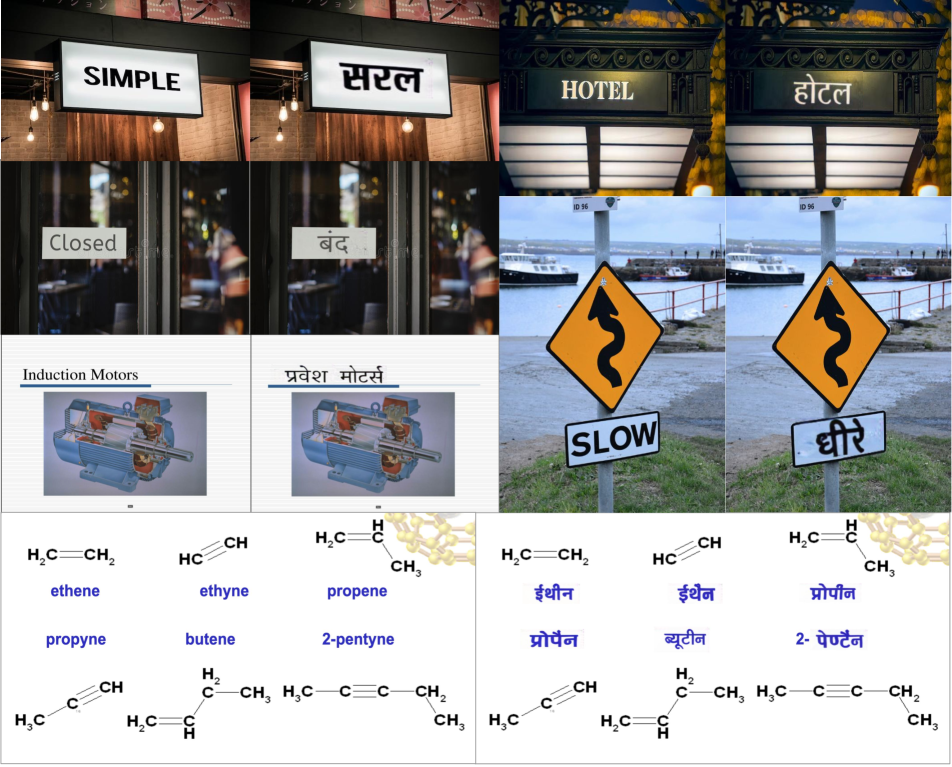
Figure 9: A selection of visual translation results for natural scene and digital-born images shown in pairs (Left/Top: source, Right/Bottom: translated). These results are verified and found correct by native speakers of these languages.

Appendix B Visual Results

We look at a few more visual results for generations from our model, VTNet in Figure 9. We perform visual translations for images from the ICDAR 2013 dataset [25], as well as a few digital-born images of memes and lecture slides created by us.

Appendix C Synthetic Dataset Generation

In this work, we introduce VT-Syn, a collection of 600K visually diverse synthetically generated scene-text samples for studying the proposed task of Visual Translation. We create this dataset using our synthetic text image generator which is a modified form of an Indic synthetic text generator [36], altered to provide more control, transformations, and paired samples in source and target languages. This generator is created using ImageMagick, an open-source image composition and editing tool.

Fonts

For the generation of texts for the six languages (English, Hindi, Chinese, Bengali, Tamil, and German), we collect a large number of open-source fonts (i.e., 560) across all languages. To be specific, the number of fonts for each language is – Hindi: 97, Chinese: 43, Bengali: 68, Tamil: 158, and English/German: 194. Next, we obtain a lexicon of 3.1K word translations for the six translation categories.

Background Images

A popular problem with scene-text editing problems is that the methods often fail to generalize to complex or detailed backgrounds [51, 40]. To handle this, we use a suitably large collection of 20K background images consisting of (i) natural scene images, (ii) textures, and (iii) plain colors. We randomly sample a background image from this large collection during the dataset generation process.

Controllable parameters

To enhance diversity in generated text images, we provide the controllable parameters of stretching, skewing, and rotating, along with other effects such as adding a shadow and color blending. We ensure these parameters reflect the realness of natural scene text.

Each generated sample consists of six images: source image ($x_{src}$), target word image ($x_{w}$), background image ($x_{bg}$), foreground image ($x_{fg}$), and target image ($x_{tgt}$). We will publicly release the dataset as well as the code to generate the VT-Syn dataset upon acceptance of this work.

References

- [1] Martin Arjovsky, Soumith Chintala, and Léon Bottou. Wasserstein generative adversarial networks. In International conference on machine learning, pages 214–223. PMLR, 2017.
- [2] Rowel Atienza. Vision transformer for fast and efficient scene text recognition. In International Conference on Document Analysis and Recognition, pages 319–334. Springer, 2021.
- [3] Dzmitry Bahdanau, Kyunghyun Cho, and Yoshua Bengio. Neural machine translation by jointly learning to align and translate. In ICLR, 2015.
- [4] Andrew Brock, Jeff Donahue, and Karen Simonyan. Large scale gan training for high fidelity natural image synthesis. arXiv preprint arXiv:1809.11096, 2018.
- [5] Hyungjin Chung, Byeongsu Sim, Dohoon Ryu, and Jong Chul Ye. Improving diffusion models for inverse problems using manifold constraints. In Advances in Neural Information Processing Systems, 2022.
- [6] Pratik Desai, Amit Sangodkar, and Om P Damani. A domain-restricted, rule based, english-hindi machine translation system based on dependency parsing. In Proceedings of the 11th international conference on natural language processing, pages 177–185, 2014.
- [7] Prafulla Dhariwal and Alexander Nichol. Diffusion models beat gans on image synthesis. Advances in Neural Information Processing Systems, 2021.
- [8] Sergey Edunov, Myle Ott, Michael Auli, and David Grangier. Understanding back-translation at scale. In EMNLP. Association for Computational Linguistics, 2018.
- [9] Angela Fan, Shruti Bhosale, Holger Schwenk, Zhiyi Ma, Ahmed El-Kishky, Siddharth Goyal, Mandeep Baines, Onur Celebi, Guillaume Wenzek, Vishrav Chaudhary, et al. Beyond english-centric multilingual machine translation. The Journal of Machine Learning Research, 22(1):4839–4886, 2021.
- [10] Jonas Gehring, Michael Auli, David Grangier, Denis Yarats, and Yann N Dauphin. Convolutional sequence to sequence learning. In International conference on machine learning, pages 1243–1252. PMLR, 2017.
- [11] Xavier Glorot and Yoshua Bengio. Understanding the difficulty of training deep feedforward neural networks. In Proceedings of the thirteenth international conference on artificial intelligence and statistics, pages 249–256. JMLR Workshop and Conference Proceeding, 2010.
- [12] Ian Goodfellow, Jean Pouget-Abadie, Mehdi Mirza, Bing Xu, David Warde-Farley, Sherjil Ozair, Aaron Courville, and Yoshua Bengio. Generative adversarial networks. Communications of the ACM, 63(11):139–144, 2020.
- [13] Google Lens Application.
- [14] Google Translate API.
- [15] Alex Graves, Santiago Fernández, Faustino Gomez, and Jürgen Schmidhuber. Connectionist temporal classification: labelling unsegmented sequence data with recurrent neural networks. In Proceedings of the 23rd international conference on Machine learning, pages 369–376, 2006.
- [16] Ishaan Gulrajani, Faruk Ahmed, Martin Arjovsky, Vincent Dumoulin, and Aaron C Courville. Improved training of wasserstein gans. Advances in neural information processing systems, 30, 2017.
- [17] Martin Heusel, Hubert Ramsauer, Thomas Unterthiner, Bernhard Nessler, and Sepp Hochreiter. Gans trained by a two time-scale update rule converge to a local nash equilibrium. Advances in neural information processing systems, 30, 2017.
- [18] Jonathan Ho, William Chan, Chitwan Saharia, Jay Whang, Ruiqi Gao, Alexey Gritsenko, Diederik P Kingma, Ben Poole, Mohammad Norouzi, David J Fleet, et al. Imagen video: High definition video generation with diffusion models. arXiv preprint arXiv:2210.02303, 2022.
- [19] Jonathan Ho, Ajay Jain, and Pieter Abbeel. Denoising diffusion probabilistic models. Advances in Neural Information Processing Systems, 33:6840–6851, 2020.
- [20] Jie Hu, Li Shen, and Gang Sun. Squeeze-and-excitation networks. In Proceedings of the IEEE conference on computer vision and pattern recognition, pages 7132–7141, 2018.
- [21] Arvi Hurskainen and Jörg Tiedemann. Rule-based machine translation from english to finnish. In Proceedings of the Second Conference on Machine Translation (WMT2017). The Association for Computational Linguistics, 2017.
- [22] Phillip Isola, Jun-Yan Zhu, Tinghui Zhou, and Alexei A Efros. Image-to-image translation with conditional adversarial networks. In Proceedings of the IEEE conference on computer vision and pattern recognition, pages 1125–1134, 2017.
- [23] Ye Jia, Ron J Weiss, Fadi Biadsy, Wolfgang Macherey, Melvin Johnson, Zhifeng Chen, and Yonghui Wu. Direct speech-to-speech translation with a sequence-to-sequence model. arXiv preprint arXiv:1904.06037, 2019.
- [24] Takatomo Kano, Sakriani Sakti, and Satoshi Nakamura. Transformer-based direct speech-to-speech translation with transcoder. In 2021 IEEE Spoken Language Technology Workshop (SLT), pages 958–965. IEEE, 2021.
- [25] Dimosthenis Karatzas, Faisal Shafait, Seiichi Uchida, M. Iwamura, Lluís Gómez i Bigorda, Sergi Robles Mestre, Joan Mas Romeu, David Fernández Mota, Jon Almazán, and Lluís-Pere de las Heras. Icdar 2013 robust reading competition. 2013 12th International Conference on Document Analysis and Recognition, pages 1484–1493, 2013.
- [26] Tero Karras, Miika Aittala, Samuli Laine, Erik Härkönen, Janne Hellsten, Jaakko Lehtinen, and Timo Aila. Alias-free generative adversarial networks. Advances in Neural Information Processing Systems, 34:852–863, 2021.
- [27] Diederik P Kingma and Max Welling. Auto-encoding variational bayes. arXiv preprint arXiv:1312.6114, 2013.
- [28] Zhifeng Kong, Wei Ping, Jiaji Huang, Kexin Zhao, and Bryan Catanzaro. Diffwave: A versatile diffusion model for audio synthesis. arXiv preprint arXiv:2009.09761, 2020.
- [29] Praveen Krishnan, Rama Kovvuri, Guan Pang, Boris Vassilev, and Tal Hassner. Textstylebrush: transfer of text aesthetics from a single example. arXiv preprint arXiv:2106.08385, 2021.
- [30] Alon Lavie, Alex Waibel, Lori Levin, Michael Finke, Donna Gates, Marsal Gavalda, Torsten Zeppenfeld, and Puming Zhan. Janus-iii: Speech-to-speech translation in multiple languages. In 1997 IEEE International Conference on Acoustics, Speech, and Signal Processing, volume 1, pages 99–102. IEEE, 1997.
- [31] Ann Lee, Peng-Jen Chen, Changhan Wang, Jiatao Gu, Sravya Popuri, Xutai Ma, Adam Polyak, Yossi Adi, Qing He, Yun Tang, et al. Direct speech-to-speech translation with discrete units. arXiv preprint arXiv:2107.05604, 2021.
- [32] Junyeop Lee, Yoonsik Kim, Seonghyeon Kim, Moonbin Yim, Seung Shin, Gayoung Lee, and Sungrae Park. Rewritenet: Reliable scene text editing with implicit decomposition of text contents and styles. arXiv preprint arXiv:2107.11041, 2021.
- [33] Ilya Loshchilov and Frank Hutter. Decoupled weight decay regularization. In 7th International Conference on Learning Representations, ICLR 2019, New Orleans, LA, USA, May 6-9, 2019. OpenReview.net, 2019.
- [34] Cheng Lu, Yuhao Zhou, Fan Bao, Jianfei Chen, Chongxuan Li, and Jun Zhu. Dpm-solver++: Fast solver for guided sampling of diffusion probabilistic models. ArXiv, abs/2211.01095, 2022.
- [35] Jiasen Lu, Dhruv Batra, Devi Parikh, and Stefan Lee. Vilbert: Pretraining task-agnostic visiolinguistic representations for vision-and-language tasks. Advances in neural information processing systems, 32, 2019.
- [36] Minesh Mathew, Mohit Jain, and CV Jawahar. Benchmarking scene text recognition in devanagari, telugu and malayalam. In 2017 14th IAPR International Conference on Document Analysis and Recognition (ICDAR), volume 7, pages 42–46. IEEE, 2017.
- [37] Satoshi Nakamura, Konstantin Markov, Hiromi Nakaiwa, Gen-ichiro Kikui, Hisashi Kawai, Takatoshi Jitsuhiro, J-S Zhang, Hirofumi Yamamoto, Eiichiro Sumita, and Seiichi Yamamoto. The atr multilingual speech-to-speech translation system. IEEE Transactions on Audio, Speech, and Language Processing, 14(2):365–376, 2006.
- [38] Alex Nichol, Heewoo Jun, Prafulla Dhariwal, Pamela Mishkin, and Mark Chen. Point-e: A system for generating 3d point clouds from complex prompts. arXiv preprint arXiv:2212.08751, 2022.
- [39] Tommi A Pirinen. Apertium-fin-eng–rule-based shallow machine translation for wmt 2019 shared task. In Proceedings of the Fourth Conference on Machine Translation (Volume 2: Shared Task Papers, Day 1), pages 335–341, 2019.
- [40] Yadong Qu, Qingfeng Tan, Hongtao Xie, Jianjun Xu, Yuxin Wang, and Yongdong Zhang. Exploring stroke-level modifications for scene text editing. arXiv preprint arXiv:2212.01982, 2022.
- [41] Prasun Roy, Saumik Bhattacharya, Subhankar Ghosh, and Umapada Pal. Stefann: scene text editor using font adaptive neural network. In Proceedings of the IEEE/CVF Conference on Computer Vision and Pattern Recognition, pages 13228–13237, 2020.
- [42] Nataniel Ruiz, Yuanzhen Li, Varun Jampani, Yael Pritch, Michael Rubinstein, and Kfir Aberman. Dreambooth: Fine tuning text-to-image diffusion models for subject-driven generation. arXiv preprint arXiv:2208.12242, 2022.
- [43] Chitwan Saharia, William Chan, Saurabh Saxena, Lala Li, Jay Whang, Emily Denton, Seyed Kamyar Seyed Ghasemipour, Burcu Karagol Ayan, S Sara Mahdavi, Rapha Gontijo Lopes, et al. Photorealistic text-to-image diffusion models with deep language understanding. arXiv preprint arXiv:2205.11487, 2022.
- [44] Abhishek Kumar Sinha, S Manthira Moorthi, and Debajyoti Dhar. Nl-ffc: Non-local fast fourier convolution for image super resolution. In Proceedings of the IEEE/CVF Conference on Computer Vision and Pattern Recognition, pages 467–476, 2022.
- [45] Jascha Sohl-Dickstein, Eric Weiss, Niru Maheswaranathan, and Surya Ganguli. Deep unsupervised learning using nonequilibrium thermodynamics. In International Conference on Machine Learning, pages 2256–2265. PMLR, 2015.
- [46] Jiaming Song, Chenlin Meng, and Stefano Ermon. Denoising diffusion implicit models. arXiv:2010.02502, October 2020.
- [47] Roman Suvorov, Elizaveta Logacheva, Anton Mashikhin, Anastasia Remizova, Arsenii Ashukha, Aleksei Silvestrov, Naejin Kong, Harshith Goka, Kiwoong Park, and Victor Lempitsky. Resolution-robust large mask inpainting with fourier convolutions. In Proceedings of the IEEE/CVF winter conference on applications of computer vision, pages 2149–2159, 2022.
- [48] Hoang Thanh-Tung and Truyen Tran. Catastrophic forgetting and mode collapse in gans. In 2020 international joint conference on neural networks (ijcnn), pages 1–10. IEEE, 2020.
- [49] Ashish Vaswani, Noam Shazeer, Niki Parmar, Jakob Uszkoreit, Llion Jones, Aidan N Gomez, Łukasz Kaiser, and Illia Polosukhin. Attention is all you need. Advances in neural information processing systems, 30, 2017.
- [50] Liang Wu, Chengquan Zhang, Jiaming Liu, Junyu Han, Jingtuo Liu, Errui Ding, and Xiang Bai. Editing text in the wild. In Proceedings of the 27th ACM international conference on multimedia, pages 1500–1508, 2019.
- [51] Qiangpeng Yang, Jun Huang, and Wei Lin. Swaptext: Image based texts transfer in scenes. In Proceedings of the IEEE/CVF Conference on Computer Vision and Pattern Recognition, pages 14700–14709, 2020.
- [52] Guangxiang Zhao, Xu Sun, Jingjing Xu, Zhiyuan Zhang, and Liangchen Luo. Muse: Parallel multi-scale attention for sequence to sequence learning. arXiv preprint arXiv:1911.09483, 2019.
- [53] Xinyu Zhou, Cong Yao, He Wen, Yuzhi Wang, Shuchang Zhou, Weiran He, and Jiajun Liang. East: an efficient and accurate scene text detector. In Proceedings of the IEEE conference on Computer Vision and Pattern Recognition, 2017.