Self-similarity and the direct (enstrophy) cascade in forced two-dimensional fluid turbulence

Abstract

A widely used statistical theory of 2D turbulence developed by Kraichnan, Leith, and Batchelor (KLB) predicts a power-law scaling for the energy, $E(k)\propto k^{\alpha}$ with an integral exponent $\alpha={-3}$, in the inertial range associated with the direct cascade. In the presence of large-scale coherent structures, a power-law scaling is observed, but the exponent often differs substantially from the value predicted by the KLB theory. Here we present a dynamical theory which describes the key physical mechanism behind the direct cascade and sheds new light on the relationship between the structure of the large-scale flow and the scaling of the small-scale structures in the inertial range. This theory also goes a step beyond KLB, to predict the upper and lower bounds of the inertial range as well as the energy scaling in the dissipation range.

1 Introduction

Fluid turbulence is a paradigm unsolved problem of classical physics and mathematics. It occupies a unique place in science due to its complicated chaotic and multiscale nature and in engineering due to its ubiquity and practical importance. The origins of turbulent cascades, which are responsible for generating structure at multiple scales are among the key mysteries. In particular, in two-dimensional (2D) turbulence, there are two different cascades: direct and inverse (Clercx & Van Heijst, 2009; Boffetta & Ecke, 2012). Specifically, the inverse cascade transfers energy from smaller to larger scales, while the direct cascade transfers enstrophy from larger to smaller scales. Here we focus on fluid flows driven at large scales, for which it is the direct cascade that is primarily responsible for the multiscale nature of turbulence.

The first theoretical, statistical description of both the inverse and direct cascade was developed by Kraichnan (1967), Leith (1968) and Batchelor (1969). In particular, for the direct cascade, the KLB theory predicts the energy density in the Fourier space to scale as a power law, $E(k)\propto k^{-3}$. Experiments (Rivera et al., 2014) and numerical simulations (Herring & McWilliams, 1985; Legras et al., 1988; Maltrud & Vallis, 1991) however generally find the spectrum to be steeper, with $E(k)$ exhibiting scaling close to a power law $k^{\alpha}$ with a non-integral exponent in the range $-5<\alpha<-3$. The deviations from the predictions of the KLB theory, which assumes the small scales to be uncorrelated, have been attributed to the presence of coherent structures, which introduce correlations. Indeed, the integral scaling exponent $\alpha=-3$ can be recovered if the coherent structures, and hence the correlations, are artificially destroyed (Benzi et al., 1988; Maltrud & Vallis, 1991; Borue, 1993; Chen et al., 2003). The importance of coherent structures, which reflect the accumulation of energy at large scales caused by the inverse cascade, has been recognized already by Kraichnan (1971) whose logarithmic correction to the $k^{-3}$ power law reflects the nonlocal nature of the direct cascade.

While no systematic description of the effects of coherent structures has been developed so far, several different mechanisms that may contribute to the direct cascade have been explored. Earlier studies have focused on the stretching of patches of vorticity, essentially treated as a passive scalar, by the neighboring vortices, leading to filamentation. In particular, Saffman (1971) predicted the exponent $\alpha=-4$ by using a simplified picture which assumed that the vorticity is uniform inside each patch and the corresponding vorticity field has a finite number of discontinuities along any straight line. Corresponding scaling, however, is only observed at early times, while on longer time scales both assumptions break down and the spectrum tends to becomes less steep (Brachet et al., 1987). It was hypothesized that, on longer time scales, vorticity filaments are stretched as they are wound up around vortices, generating a fractal structure that is characterized by a nonintegral exponent. For point vortices, the corresponding exponent was predicted to be $\alpha=-11/3=-3.6(6)$ (Moffatt, 1986; Gilbert, 1988). While these results established a relationship between the topology of the large-scale flow and the scaling exponent, they did not explain the lack of universality observed in the presence of coherent structures. Indeed, coherent structures feature vortices with a wide variety of shapes and hence stretching properties (Zhigunov & Grigoriev, 2022).

More recent studies have identified straining regions of large-scale flows, rather than vortices, as playing a key role in the direct cascade. Numerical results of Chen et al. (2003) suggest that the primary physical mechanism behind the direct cascade is “vortex thinning,” i.e., steepening of the vorticity gradients in strain-dominated regions of the flow. This picture is supported by the experimental studies of Kelley & Ouellette (2011) and Liao & Ouellette (2015) which found that, at small scales, the spectral fluxes of both the energy and the enstrophy are enhanced in regions that are predominantly straining. This relation is particularly clear in numerical simulations of body-forced turbulence on a square doubly periodic domain where the large-scale flow at high Reynolds numbers ($Re$) is dominated by a pair of counter-rotating vortices, and vorticity filaments are mostly found in the straining regions (Zhigunov & Grigoriev, 2022). The presence of pronounced coherent structures in this flow leads to particularly strong deviations from the KLB predictions, with the scaling exponent reaching values as high as $\alpha\approx-5$. While convincing, this evidence is qualitative, and a quantitative theory is yet to be developed that can explain and predict the scaling exponents found in both numerics and experiments and their connection to the spatial and temporal properties of coherent structures.

This paper introduces the key elements of such a quantitative theory for bounded flows that reach statistical equilibrium in the presence of driving and dissipation. The paper is structured as follows. We will start by analyzing the large- and small-scale structures of vorticity that emerge in direct numerical simulations of high-$Re$ 2D flows in Section 2. Section 3 introduces self-similar solutions of the Euler equation describing vortex thinning in the inertial range. The Fourier spectra of these self-similar solutions and the associated energy and enstrophy fields are computed in Section 4. The results are discussed in Section 5 and conclusions are presented in Section 6.

2 High-$Re$ flow in two dimensions

To gain intuition into the physical mechanism of the direct cascade, it is helpful to analyze typical vorticity structures that emerge in high-$Re$ incompressible flows driven by steady large-scale forcing on a doubly periodic domain ($0\leq x,y<2\pi$). Such flows can be described by the Navier-Stokes equation

$$\partial_{t}{\omega}+{\bf u}\cdot\nabla{\bf\omega}=\nu\nabla^{2}{\omega}+\varphi,$$ (1)

written in terms of vorticity $\omega=\partial_{x}u_{y}-\partial_{y}u_{x}=-\nabla^{2}\psi$, where $u_{x}=\partial_{y}\psi$ and $u_{y}=-\partial_{x}\psi$ are the velocity components, $\psi$ is the stream function, and $\varphi$ describes the external forcing. In this section, we will focus on the results of numerical simulations of turbulent flow with $\nu=10^{-5}$ driven by a steady checkerboard forcing $\varphi=\sin(4x)\sin(4y)$ reported by Zhigunov & Grigoriev (2022). The forcing wavenumber $k_{f}=4\sqrt{2}$ was chosen to be sufficiently low to make sure there is a large separation between the forcing scale and the Taylor microscale $\ell_{t}=Re^{-1/2}\ell_{0}$ at which viscous effects become important. Here, the Reynolds number is defined as $Re=\mathcal{E}\ell_{0}^{2}/\nu$, where $\mathcal{E}$ describes the characteristic magnitude of velocity gradient tensor elements $\partial_{i}u_{j}$, and the characteristic length scale $\ell_{0}$ and velocity scale $\mathcal{E}\ell_{0}$ are both $O(1)$, so that $\ell_{t}=(\nu/\mathcal{E})^{1/2}$. To make sure the small-scale structures are resolved, the flow was computed on a grid with resolution $2048\times 2048$. Accounting for the 2/3 dealiasing used in the numerical simulations, this corresponds to the highest resolved wavenumber of $k_{max}=682$.

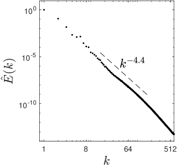
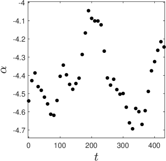
Figure 1: The energy of a turbulent flow. (a) The energy spectrum averaged over a long time interval ($10^{3}$ nondimensional units). (b) The exponent of the spectrum show at intervals of the characteristic time scale $T_{c}=10$, averaged with nearby points.

The large-scale flow is found to be insensitive to the particular choice of the forcing profile, so long as its frequency is relatively low (Kim & Okamoto, 2010, 2015; Kim et al., 2017). This is due to the accumulation of the energy at the largest scales accessible to the flow, as illustrated by Figure 1(a), caused by the inverse cascade. The energy spectrum averaged over a long time interval is found to exhibit a power-law scaling $E(k)\propto k^{\alpha}$ over roughly a decade in the wavenumber ($16\leq k\leq 170$). This scaling indicates the presence of an inertial range characteristic of fully developed turbulence. The exponent $\alpha\approx-4.4$ is found to be quite different from that predicted by KLB theory.

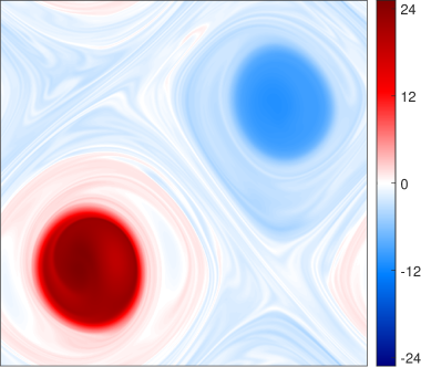
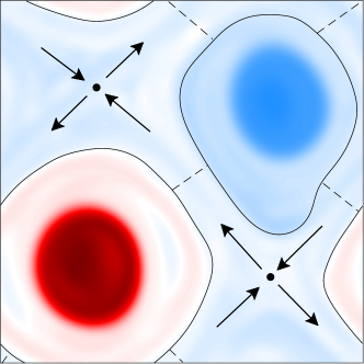
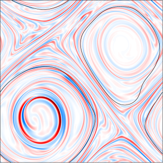
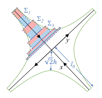
Figure 2: Typical snapshot of a High-$Re$ turbulent flow. (a) Vorticity field $\omega$. (b) The large-scale component of $\omega$ (corresponding to wavenumbers $k\leq 16$) features two pronounced counter-rotating vortices. The boundaries between regions dominated by vortical and straining flow are shown as solid black lines and the boundaries between the two hyperbolic regions are shown as dashed black lines. The arrows indicate the direction of the flow in each hyperbolic region and the corresponding stagnation points are shown as black circles. Everything is shown in a reference frame co-moving with the large-scale vortex pattern. (c) The small-scale component of $\omega$ (corresponding to wavenumbers $k\geq 16$) features pronounced vorticity filaments. (d) The local coordinate system and geometry of a hyperbolic region of the flow. The color map in all four panels uses red (blue) shades to indicate positive (negative) values of vorticity.

Figure 2(a) shows a typical snapshot of the turbulent flow. We decomposed this flow into a small-scale and large-scale component by applying a filter which corresponds to a smoothed circular window with radius $O(k_{f})$ in Fourier space, so the entire inertial range is included in the small-scale component. Several features of this flow are worth pointing out. The large-scale flow shown in Figure 2(b) is organized by a pair of counter-rotating vortices. The region outside the vortex cores is dominated by the straining flow, with the strain driven by the two vortices. The region of straining flow has vorticity which is nearly uniform. The large-scale flow is not static, rather, a large fraction of the time, it is found to be nearly time-periodic (Zhigunov & Grigoriev, 2022). Although time-dependent, the flow structure remains largely unchanged, with both vortices executing a nearly circular motion. There are four stagnation points, a pair of elliptic ones inside the vortex cores and another pair of hyperbolic ones inside the region of straining flow outside of the vortex cores. When averaged over the characteristic time scale $T_{c}\approx 10$, which corresponds to the approximate period of the large-scale flow, the energy spectrum retains a power-law shape. However, the associated exponent $\alpha$ is found to vary over a significant range of values, as Figure 1(b) shows, reflecting the changes in the properties of the large-scale flow on time scales longer than $T_{c}$.

These results appear to be quite representative. Similar large-scale coherent structures in the form of “vortex crystals” (Aref et al., 2003) are also found to form for flows forced at small scales (Smith & Yakhot, 1994; Chertkov et al., 2007), even though they tend to take a rather long time to emerge. Notably, this behavior characteristic of forced turbulence is quite different from that found for freely decaying turbulence (McWilliams, 1984; Bracco et al., 2000) where pronounced coherent structures fail to form.

Most of the small-scale vorticity has filamentary structure with the filaments mostly confined to the region of straining flow, as illustrated by Figure 2(c). This region can be decomposed into a pair of hyperbolic regions, each one containing a hyperbolic stagnation point. Inside each hyperbolic region, the filaments are mostly oriented along the extending direction of the straining flow, although some filaments are found to be oriented along the contracting direction. Some filamentary vorticity is also found inside the vortex cores. These filaments are found predominantly in the regions where the gradient of the large-scale vorticity is the largest and are oriented transversely to this gradient. Hence, both the straining and vortical regions contribute to the direct cascade, with the former corresponding to the picture described by Kraichnan (1971) and the latter corresponding to the picture described by Moffatt (1986) and Gilbert (1988). We will focus here on the straining region which contains most of the filamentary vorticity.

3 Self-similar solutions and the direct cascade

In the inertial range $k_{f}\ll k\ll k_{t}$, both the forcing and the viscous dissipation can be ignored, so the flow is effectively described by the Euler equation

$$\partial_{t}\omega+{\bf u}\cdot\nabla\omega=0.$$ (2)

As discussed in the previous section, inside each hyperbolic region, the large-scale flow has essentially constant vorticity. Consider a reference frame in which a hyperbolic stagnation point remains at the origin and an orthogonal coordinate system with the $y$ coordinate oriented along the extending direction of the flow, as shown in Figure 2(d). The velocity ${\bf u}_{l}$ of the large-scale flow inside the hyperbolic region can be written as

$${\bf u}_{l}=-\mathcal{E}x\hat{x}+\mathcal{E}(y+2\cot(\theta)x)\hat{y},$$ (3)

where $\mathcal{E}$ is the strain rate and $\theta$ is the angle between the extending and contracting direction, hence the large-scale vorticity in the hyperbolic region is simply $\omega_{l}=2\mathcal{E}\cot\theta$. For the simulations considered here, the time-dependence of the large-scale flow manifests mostly as a slow overall drift of the pattern, hence the strain rate $\mathcal{E}>0$, the orientation of the $y$ axis, and the angle $\theta$ can be considered constant (or at least slowly varying). This limit correspond to the adiabatic approximation used by Lapeyre et al. (1999, 2001).

Separating the flow into the large- and small-scale contributions and substituting the result into the Euler equation yields

$$\partial_{t}\omega_{s}+{\bf u}_{l}\cdot\nabla\omega_{s}=-{\bf u}_{s}\cdot\nabla\omega_{s}.$$ (4)

This evolution equation shows that small-scale vorticity $\omega_{s}$ can be considered a passive scalar that is advected by the large-scale flow ${\bf u}_{l}$, as is commonly assumed (Kraichnan, 1971), only when the term ${\bf u}_{s}\cdot\nabla\omega_{s}$ vanishes. Indeed, when the level sets of the streamfunction $\psi_{s}$ describing the small-scale component of the flow are aligned with the level sets of the small-scale vorticity $\omega_{s}$, the right-hand-side of Equation (4) disappears, so small-scale vorticity effectively becomes a passive scalar. This will be the case for vorticity filaments whose radius of curvature is large compared with their thickness. As Figure 2(c) illustrates, this condition is satisfied almost everywhere except for the small regions where the filaments are folded sharply.

In practice, the extending and contracting directions of the straining flow tend to be nearly orthogonal so, without loss of generality, we will assume $\theta=\pi/2$ in most of the discussion below. The corresponding streamfunction then becomes $\psi_{l}=-\mathcal{E}xy$ and the large-scale vorticity vanishes, $\omega_{l}=0$. Inside the hyperbolic region

$$|xy|\lesssim h^{2},$$ (5)

bounded by the level sets of $\psi_{l}$, Equation (4) reduces to

$$\partial_{t}\omega-\mathcal{E}x\partial_{x}\omega+\mathcal{E}y\partial_{y}\omega=0.$$ (6)

The shape (and the characteristic thickness $h$) of the hyperbolic region depends on the properties of the large-scale flow. As illustrated by Figure 2(b), the hyperbolic region does not have to be reflection-symmetric with respect to either the extending or contracting direction. We assume it to be symmetric, without loss of generality, to simplify the notations. The general solution to the linear equation (6) can be found using the method of characteristics

$$\omega=g(\chi,\eta),$$ (7)

where $g$ are arbitrary functions of the similarity variables $\chi=\ln|x|+\mathcal{E}t$ and $\eta=\ln|y|-\mathcal{E}t$. This family of solutions is dynamically self-similar, i.e., $\omega(e^{\mathcal{E}T}x,e^{-\mathcal{E}T}y,t)=\omega(x,y,t+T)$ for any $T$.

Consider, for instance, small-scale vorticity filaments oriented along the extending direction, in which case

$$\omega=g_{c}^{\pm}(\chi),$$ (8)

where the superscript denotes the sign of $x$. This family of solutions describes vortex thinning associated with stretching of filaments as they are advected towards the $y$ axis. The functions $g_{c}^{\pm}(\chi)$ are determined by the variation in the vorticity field at the “entrances” to the hyperbolic region where $x=\pm\ell_{0}$. Since vorticity at $x=\ell_{0}$ and $x=-\ell_{0}$ will generally be different, so $g_{c}^{+}(\chi)$ and $g_{c}^{-}(\chi)$ will also be different. These self-similar solutions describe vorticity filaments whose characteristic thickness decreases exponentially fast, $\Delta x(t)\propto e^{-\mathcal{E}t}$.

For a time-periodic large-scale flow with period $T$, the vorticity field at the entrances to the hyperbolic region will also be time-periodic. As a result, we will have $\omega(x,t+T)=\omega(x,t)$ inside the hyperbolic region as well. Under these conditions, Equation 8 describes a vorticity field which is self-similar in the conventional sense, i.e., $\omega(\Lambda x,t)=\omega(x,t)$, where $\Lambda=e^{\mathcal{E}T}>1$ and $|x|<\ell_{0}/\Lambda$. This is illustrated in Figure 2(d); the vorticity field inside the region $\Sigma_{1}$ is compressed along the $x$ direction and stretched in the $y$ direction by the same factor $\Lambda$ after one period and mapped onto the region $\Sigma_{2}$. Similarly, the region $\Sigma_{2}$ is mapped onto the region $\Sigma_{3}$, etc. In the remainder of this paper, we will focus on the spectral properties of vorticity fields described by such self-similar solutions which describe the flux of enstrophy towards smaller scales.

In conclusion of this section, for completeness, we should point out the existence of another family of self-similar solutions

$$\omega=g_{e}^{\pm}(\eta),$$ (9)

where $g_{e}^{\pm}(\eta)$ are again arbitrary functions and the superscript denotes the sign of $y$. This family of solutions describes vorticity filaments oriented along the contracting direction of the straining flow. These filaments become thicker, rather than thinner, with their characteristic thickness growing as $\Delta y(t)\propto e^{\mathcal{E}t}$, hence this family of solutions describes so-called backscatter, or flux of enstrophy towards larger scales. For time-periodic large-scale flow, the corresponding small-scale vorticity field is also self-similar, $\omega(\Lambda^{-1}y,t)=\omega(y,t+T)$. Such solutions will only be dynamically relevant when the vorticity at the entrance of the hyperbolic region varies slowly in the $x$ and quickly in the $y$ direction. Indeed, this is commonly found to be the case in turbulent flow as illustrated in Figure 2(c). We will delay the discussion of backscatter until Section 5.

4 Fourier spectra

As discussed in the previous section, the flux of enstrophy towards small scales can be described by a dynamically self-similar vorticity field which belongs to the family defined by Equation (8). For a time-periodic large-scale flow with period $T=2\pi/\Omega$, the self-similar solution becomes periodic in the similarity variable $\chi$ and can be expanded as a Fourier series

$$\omega=\sum_{n=1}^{\infty}a_{n0}^{\pm}\cos[ns\chi+\phi_{n0}^{\pm}]=\sum_{n=1}^{\infty}a_{n0}^{\pm}\cos[ns\ln|x|+n\Omega t+\phi_{n0}^{\pm}],$$ (10)

where $s=\Omega/\mathcal{E}=2\pi/\ln(\Lambda)$, $a_{n0}^{\pm}$ are the Fourier amplitudes, and $\phi_{n0}^{\pm}$ are the corresponding phases. Note that, in the co-moving reference frame, the forcing $\varphi$ acquires time-dependence; the amplitudes $a_{n0}^{\pm}$ and phases $\phi_{n0}^{\pm}$ are determined by the spatial and temporal profile of this time-dependent forcing. Before proceeding to compute the enstrophy spectrum associated with the small-scale vorticity component, let us consider the effect of finite viscosity.

4.1 Effect of viscosity

In the presence of viscosity, self-similarity of the small-scale vorticity field in a hyperbolic region will break down when the filament thickness becomes comparable to the Taylor microscale $\ell_{t}$. Equation (6) should be replaced with

$$\partial_{t}\omega-\mathcal{E}x\partial_{x}\omega-\nu\partial_{x}^{2}\omega=0.$$ (11)

Small viscosity implies that the ratio $\epsilon=\nu/\mathcal{E}=\ell_{t}^{2}$ is small compared with $\ell_{0}^{2}$. In the inertial range, the product $\epsilon x^{-2}=(\ell_{t}/x)^{2}\ll 1$, and we can represent the effect of viscosity perturbatively using a WKB expansion

$$\omega=\frac{1}{2}\sum_{n=1}^{\infty}a_{n0}^{\pm}\exp\left[\Theta_{n0}(\chi)+\epsilon x^{-2}\Theta_{n1}(\chi)+\epsilon^{2}x^{-4}\Theta_{n2}(\chi)+\cdots\right]+\text{c.c.},$$ (12)

where c.c. denotes complex conjugate. For $\epsilon=0$, the corrections disappear and we should recover the inviscid solution (10), hence

$$\Theta_{n0}(\chi)=ins\chi+i\phi^{\pm}_{n0}=ins\ln|x|+in\Omega t+i\phi^{\pm}_{n0}.$$ (13)

Substituting (12) into (11) and collecting terms of different orders in $\epsilon$, we find

$$\Theta_{n1}(\chi) =\frac{\Theta_{n0}^{\prime\prime}(\chi)+\Theta_{n0}^{\prime}(\chi)[\Theta_{n0}^{\prime}(\chi)-1]}{2},$$ (14)

etc. Substituting the expression for $\Theta_{n0}(\chi)$ into this equation, we find

$$\Theta_{n1} =\frac{-ins-n^{2}s^{2}}{2}.$$ (15)

The vorticity is therefore given by the spatially modulated version of the original self-similar solution

$$\omega(x,t)\approx\sum\limits_{n=1}^{\infty}a_{n}^{\pm}(x)\cos\left[ns\ln|x|+n\Omega t+\phi_{n}(x)\right],$$ (16)

where, to leading order in $\ell_{t}/x$,

$$\phi_{n}^{\pm}(x)=\phi^{\pm}_{n0}-\frac{ns}{2}\frac{\ell_{t}^{2}}{x^{2}}$$ (17)

and

$$a_{n}^{\pm}(x)=a_{n0}^{\pm}\exp\left[-\frac{n^{2}s^{2}}{2}\frac{\ell_{t}^{2}}{x^{2}}\right].$$ (18)

As expected, we recover the original self-similar solution in the inertial range, $|x|\gg\ell_{t}$, while, in the dissipation range, $|x|\lesssim\ell_{t}$, its amplitude becomes strongly attenuated. It is straightforward to compute the solutions to a higher order in perturbation theory although additional corrections have a minor effect in both the inertial range and the dissipation range.

4.2 Enstrophy spectrum

To determine the scaling of enstrophy, recall that small-scale vorticity is confined to the hyperbolic regions of the large-scale flow, with each hyperbolic region giving essentially the same contribution. This confinement can be represented by making the amplitudes $a_{n}^{\pm}$ a function of both $x$ and $y$. The streamlines of the large-scale flow correspond to constant values of the product $xy$ so, in the absence of viscosity, the amplitudes should be a function of $xy$. Here we will assume a Gaussian profile, so that, in the presence of viscosity,

$$a_{n}(x,y)=a_{n0}^{\pm}\exp\left[-\frac{n^{2}s^{2}}{2}\frac{\ell_{t}^{2}}{x^{2}}-\frac{x^{2}y^{2}}{h^{4}}\right],$$ (19)

although other choices will yield qualitatively similar results. The corresponding vorticity field is shown in Figure 3(a) for the special case of solution (10)

$$\omega=\cos(s\chi)$$ (20)

used here for illustration purposes.

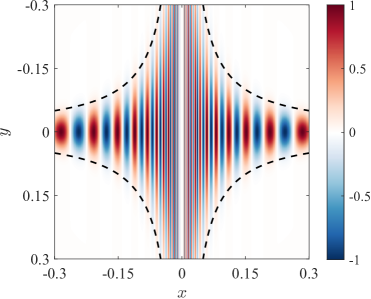
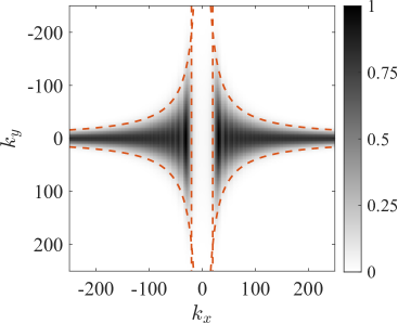
Figure 3: A snapshot of the vorticity field $\omega({\bf x},t)$ defined by Eq. (20) in the physical space for $s=20$, $h=0.1$, $\ell_{0}=1$, and $Re=10^{7}$ (a). The black dashed line represents the boundary of the hyperbolic region given by inequality (5). The corresponding (normalized) power spectrum $\hat{H}({\bf k})$ (b). The boundaries defined by Equations (36) and (37) are shown as red dashed lines.

The Fourier spectrum of the vorticity field corresponding to the general solution (10) is given by

$$\hat{\omega}({\bf k},t) \approx\sum\limits_{n=1}^{\infty}\frac{a_{n0}^{-}}{2}\int_{-\ell_{0}}^{0}dx\int_{-\ell_{0}}^{\ell_{0}}dy\exp\left[f_{ns}({\bf k},{\bf x})+in\Omega t+i\phi_{n0}^{-}\right]$$

$$+\sum\limits_{n=1}^{\infty}\frac{a_{n0}^{+}}{2}\int_{0}^{\ell_{0}}dx\int_{-\ell_{0}}^{\ell_{0}}dy\exp\left[f_{ns}({\bf k},{\bf x})+in\Omega t+i\phi_{n0}^{+}\right]+\textit{c.c.},$$ (21)

where

$$f_{r}({\bf k},{\bf x})=ir\ln|x|-\frac{ir+r^{2}}{2k_{t}^{2}x^{2}}-\frac{x^{2}y^{2}}{h^{4}}+i{\bf k}\cdot{\bf x},$$ (22)

and we have defined the characteristic wavenumber $k_{t}=1/\ell_{t}$ corresponding to the Taylor microscale. The integrals can be evaluated using the saddle-point approximation. The saddle point ${\bf x}_{s}$ is found by solving the equation $\nabla f_{r}({\bf k},{\bf x}_{s})=0$,

$$x_{s} =-\frac{r}{k_{x}}X(\beta_{r}),$$

$$y_{s} =\frac{ik_{y}h^{4}}{2x_{s}^{2}}.$$ (23)

Here $X(\beta)$ is the dominant root of the cubic equation $X^{2}-X^{3}+\beta=0$ which corresponds to the limit $X(0)=1$,

$$\beta_{r}=-i\frac{\alpha}{2r^{3}}+\frac{1-ir}{r^{2}}\kappa^{2},$$ (24)

and we introduced the short-hand notations $\kappa=k_{x}/k_{t}$ and $\alpha=k_{x}^{2}k_{y}^{2}h^{4}$.

So long as $\left|\textit{Re}[x_{s}]\right|<\ell_{0}$, the saddle point approximation yields

$$\hat{\omega}({\bf k},t) \approx\sum\limits_{n=1}^{\infty}\frac{\pi a_{n0}^{-}\exp\left[f_{ns}({\bf k},{\bf x}_{s})+in\Omega t+i\phi_{n0}^{-}\right]}{2\sqrt{-g_{ns}({\bf k},{\bf x}_{s})}}$$

$$+\sum\limits_{n=1}^{\infty}\frac{\pi a_{n0}^{+}\exp\left[f_{ns}({\bf k},{\bf x}_{s})+in\Omega t+i\phi_{n0}^{+}\right]}{2\sqrt{-g_{ns}({\bf k},{\bf x}_{s})}}+\textit{c.c.}$$ (25)

where

$$f_{r}({\bf k},{\bf x}_{s}) =ir\ln\left|\frac{r}{k_{x}}\right|+irF(\beta_{r}),$$

$$F(\beta) =\ln X(\beta)-X(\beta)-\frac{\beta}{2X^{2}(\beta)}$$ (26)

and

$$g_{r}({\bf k},{\bf x}_{s}) =\det(\nabla\nabla f_{r})|_{{\bf x}_{s}}=\frac{irG(\beta_{r})}{h^{4}},$$

$$G(\beta) =2+6\frac{\beta}{X^{2}(\beta)}.$$ (27)

Let us define the average of the enstrophy spectrum over a period of the large-scale flow

$$\hat{H}(\mathbf{k})=\frac{1}{T}\int_{0}^{T}|\hat{\omega}({\bf k},t)|^{2}dt.$$ (28)

Using appropriate orthogonality relations, we find

$$\hat{H}(\mathbf{k})\approx 2\pi^{2}h^{4}\sum_{n=1}^{\infty}H_{n}A(ns,\alpha_{n},\kappa),$$ (29)

where

$$H_{n}=\frac{1}{4}\left|a_{n0}^{-}e^{i\phi_{n0}^{-}}+a_{n0}^{+}e^{i\phi_{n0}^{+}}\right|^{2}$$ (30)

and the wavenumber dependence is contained entirely in the amplitudes

$$A(r,\alpha,\kappa)=\frac{e^{\text{Re}[2f_{r}]}}{r|G(\beta_{r})|}.$$ (31)

Note that, in the absence of viscosity, the enstrophy spectrum depends on the wavenumber only through the nondimensional combination $\alpha$, with the amplitude $A(r,\alpha,\kappa)$ being a decreasing function of $\alpha$. Therefore, at high $Re$, the enstrophy is confined to a hyperbolic region in the Fourier space as well, as illustrated in Figure 3(b). The width of the hyperbolic region can be easily estimated in various limiting cases. In the limit of $r$-large, $\beta$ is small and we can use the Taylor expansion

$$X(\beta)=1+\beta-2\beta^{2}+\cdots.$$ (32)

Keeping the leading order terms in $\beta$, we find an explicit expression for the amplitude

$$A(r,\alpha,\kappa)\approx\frac{1}{2r}\exp\left[-\frac{\alpha}{2r^{2}}-\kappa^{2}\right].$$ (33)

The approximation (32) is accurate for $r\gtrsim 10$, but it starts to break down for smaller values of $r$, especially when $\kappa$ is low. This is illustrated in Figure 4 which compares this approximation with the exact result (31) for $\kappa=0.1$ and $\kappa=2$ representative of the inertial and dissipation range, respectively. For $r$-small, one should instead consider the limit of $\beta$-large where

$$X(\beta)=\beta^{1/3}+\frac{1}{3}+\frac{1}{9}\beta^{-1/3}+\cdots$$ (34)

and, to leading order in $\beta$,

$$A(r,\alpha,\kappa)\approx\frac{1}{6r\left|\beta_{r}^{1/3}\right|}\exp\left[-3r\text{Re}\left[i\beta_{r}^{1/3}\right]\right].$$ (35)

This approximation is found to be accurate for $r\lesssim 0.1$, as illustrated in Figure 4.

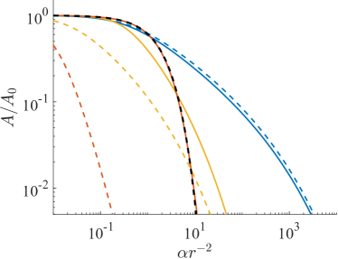
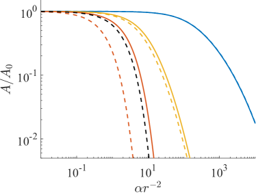
Figure 4: The amplitude function $A(r,\alpha,\kappa)$, normalized by $A_{0}=A(r,0,\kappa)$, for $\kappa=0.1$ (a) and $\kappa=2$ (b) with $r=20$ (red), $r=1$ (yellow), and $r=0.05$ (blue). The results based on the exact solution $X(\beta)$ (solid lines) are compared with those based on the power series expansion of $X(\beta)$ in the limits of low $\beta$ (black dashed line) and high $\beta$ (colored dashed lines).

Let $\bar{n}$ be the dominant harmonic in the Fourier series (10) and $\bar{r}\equiv\bar{n}s$. In the inertial range, the amplitude (35) becomes independent of $r$, hence the hyperbolic region is defined by the inequality

$$|k_{x}k_{y}|\lesssim\frac{z(\bar{r})}{h^{2}},\qquad z(\bar{r})=\begin{cases}1,&\bar{r}\lesssim 0.1,\\ 2\bar{r},&\bar{r}\gtrsim 10.\end{cases}$$ (36)

Furthermore, the saddle-point approximation which underlies Equation (31) is only accurate when the saddle lies inside the integration domain, i.e., $|x_{s}|<\ell_{0}$ which corresponds to

$$|k_{x}|\gtrsim k_{s}\equiv\frac{\bar{r}}{\ell_{0}}.$$ (37)

For $|k_{x}|<k_{s}$, the amplitude $A(r,\alpha,\kappa)$ becomes exponentially small. As Figure 3(b) illustrates, the inequalities (36) and $\eqref{eq:ks}$ describe well the boundaries of the region in the Fourier space outside of which the enstrophy spectrum essentially vanishes. The maximal width of the enstrophy spectrum in the $k_{y}$ direction can be estimated by setting $k_{x}=k_{s}$ in Equation (36), yielding

$$\max_{k_{x}}|k_{y}|\lesssim k_{h}\equiv\frac{z(\bar{r})\ell_{0}}{\bar{r}h^{2}}.$$ (38)

The enstrophy scaling can be determined by integrating $\hat{H}(\mathbf{k})$ over the annular region $k<|{\bf k}|<k+dk$. For $k\gtrsim\max(k_{s},k_{h})$, the dominant contribution to the integral comes from the two arcs near the $k_{x}$ axis where the annular region intersects the hyperbolic region defined by the inequality (36). For $k\gtrsim k_{a}$, where

$$k_{a}\equiv\frac{2\sqrt{2\bar{r}}}{h},$$ (39)

these arcs are well-approximated by straight lines with $k_{x}=k$, such that

$$H(k)=4\pi^{2}h^{2}\sum\limits_{n=1}^{\infty}H_{n}\left[\int_{0}^{\infty}A(ns,\alpha,\kappa)\frac{d\alpha}{\sqrt{\alpha}}\right]_{k_{x}=k}\,k^{-1}.$$ (40)

In the inertial range, we can set $\kappa=0$, so the expression in square brackets becomes $k$-independent and we find $H(k)\propto k^{-1}$, as predicted by the KLB theory.

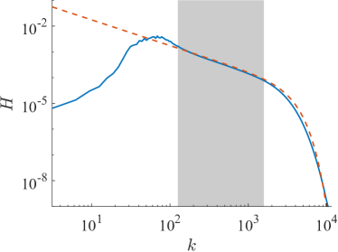
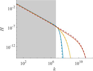
Figure 5: The enstrophy spectrum $H(k)$. (a) The result obtained by direct numerical evaluation of the time-average (28), shown as a solid blue line, is compared with the analytical result (41), shown as a dashed red line, for the vorticity field (20) with $s=20$, $h=0.1$, $\ell_{0}=1$, and $Re=10^{7}$. (b) The spectrum calculated using the saddle-point approximation (40) for $s=20$ (blue), $s=2$ (yellow), and $s=0.2$ (red) and $Re=10^{12}$ (solid lines). Dashed lines show the fits to an expression of the form $H\propto\exp{(-b(k/k_{t})^{\gamma})}k^{-1}$, where $b=1$ and $\gamma=2$ for $s=20$; $b=0.74$ and $\gamma=0.71$ for $s=1$; $b=0.018$ and $\gamma=2/3$ for $s=0.05$. In both panels, gray background represents the inertial range whose boundaries are given by Equations (43) and (44).

Further progress can be made in various limiting cases. For $s$-large, the integral in (40) can be evaluated with the help of (33), yielding

$$H(k)=2\pi^{5/2}h^{2}\sum_{n=1}^{\infty}H_{n}e^{-(k/k_{t})^{2}}k^{-1}$$ (41)

with the Gaussian envelope describing the effect of viscosity. The corresponding energy spectrum is given by

$$E(k) \propto k^{-2}H(k)\propto e^{-(k/k_{t})^{2}}\,k^{-3}.$$ (42)

The analytical result (41) accurately represents the enstrophy spectrum computed numerically in both the inertial and dissipation range, as Figure 5(a) illustrates. As expected, the boundary between these two regions is defined by the Taylor microscale $k_{t}=\ell_{t}^{-1}=Re^{1/2}\ell_{0}^{-1}$. Noticeable deviations from power-law scaling are found for $k\gtrsim k_{d}$, where

$$k_{d}=\frac{k_{t}}{2}.$$ (43)

s The low-wavenumber boundary of the inertial range should be described by

$$k_{c}\equiv\max\left(k_{s},k_{h},k_{a}\right).$$ (44)

Both boundaries are indeed in good agreement with the numerically computed spectra corresponding to the self-similar vorticity field (20) as can be seen in Figure 5. Note that, in the limit of $s\to 0$, $k_{c}=k_{h}\propto s^{-1}$, while, in the limit $s\to\infty$, $k_{c}=k_{s}\propto s$. Hence, the inertial range should be the widest for intermediate values of $s$.

For $s$-small, the integrals in (40) can be evaluated using the approximation (35) for $1\leq n\leq n_{\text{max}}$, where $n_{\text{max}}\sim 0.1/s$. The integrals are dominated by values of $\alpha$ much smaller than unity, and, in this limit, we can use a series expansion

$$3r\beta_{r}^{1/3}\approx-c_{1,r}\kappa^{2/3}-c_{2,r}\alpha\kappa^{-4/3},$$ (45)

where we have defined the coefficients $c_{1,r}=-3(r-ir^{2})^{1/3}$ and $c_{2,r}=\frac{i}{2}(r-ir^{2})^{-2/3}$. Assuming the series (10) truncated at $n_{\text{max}}$ accurately describes the small-scale vorticity field, we can write

$$H(k)\approx\sum_{n=1}^{n_{\textit{max}}}\int_{0}^{\infty}\frac{2\pi^{2}H_{n}h^{4}}{|c_{1,ns}|\kappa^{2/3}}\exp{\left[-\mathrm{Im}(c_{1,ns})\kappa^{2/3}-\mathrm{Im}(c_{2,ns})\frac{\alpha}{\kappa^{4/3}}\right]}\frac{d\alpha}{\sqrt{\alpha}}.$$ (46)

Evaluating the integrals with the help of the saddle node approximation, we find

$$H(k)\approx\frac{2^{3/2}\pi^{5/2}h^{2}}{\sqrt{3}}\sum_{n=1}^{n_{\textit{max}}}H_{n}e^{-\mathrm{Im}(c_{1,ns})(k/k_{t})^{2/3}}k^{-1},$$ (47)

where we used the relation $|c_{1,r}|\,[\mathrm{Im}(c_{2,r})]^{1/2}\approx\sqrt{3/2}$ which holds at small values of $r$. It should be pointed out that, for $s$-small and $\max(k_{s},k_{a})<k<k_{h}$, the integral of $\hat{H}({\bf k})$ over the annular region should include the contribution from the hyperbolic region near the $k_{y}$-axis, which would require a correction to Equation (40). This correction should be relatively small and therefore is not considered here.

The accuracy of the approximations (41) and (47) can be confirmed by comparing them with the integral (40) evaluated numerically. Figure 5(b) shows the respective results computed for the vorticity field (20). For both $s=20$ and $s=0.05$, the enstrophy spectrum is indeed well-described by the analytical results (41) and (47), respectively. While both approximations break down at the intermediate values of $s$, we can leverage the functional form of these approximations to speculate that the enstrophy spectrum generally has the form

$$H(k)\propto e^{-b(s)\,(k/k_{t})^{\gamma(s)}}\,k^{-1},$$ (48)

where the exponent $\gamma$ interpolates between the values of $2/3$ and 2 for $s$-low and $s$-high, respectively. For the intermediate value $s=1$, we find the spectrum can indeed be fitted quite well by this expression with $b=0.74$ and $\gamma=0.71$.

The theory presented here clearly is not directly applicable to the DNS discussed in Section 2. For instance, the predicted exponent $\alpha=-3$ is substantially different from the observed value $\alpha=-4.4$ describing the long-time average. Nonetheless, some of the observations are in reasonable agreement with the predictions. In the DNS, we find $\mathcal{E}\approx 3.7$, $\Omega\approx 0.63$, $\ell_{0}=2\sqrt{2}\pi/4\approx 2.2$, $h\approx 1$, and $\bar{n}=1$, with the largest uncertainty in the value of $h$. This yields $\bar{r}=s\approx 0.17$, $Re\approx 3.7\times 10^{5}$, $k_{t}\approx 608$, $k_{s}\approx 0.07$, $k_{h}\approx 13$, and $k_{a}\approx 1.2$. Indeed, the energy spectrum shown in Figure 1(a) is found to be reasonably close to a power law in the predicted inertial range $k_{c}<k<k_{d}$, where $k_{c}\approx 13$ and $k_{d}\approx 304$. The deviation from power-law scaling in the predicted dissipation range $k>k_{d}$ is found to be fairly weak, consistent with the low value of $s$, as illustrated in Figure 5(b). A quantitative comparison of the predicted and observed scaling in the dissipation range would require $k_{\text{max}}\gg k_{t}$ and hence a far finer mesh than that used in our DNS (which corresponds to $k_{\text{max}}\approx 1.1k_{t}$).

4.3 Effect of the angle between extending and contracting directions

In the analysis above, we assumed the extending and contracting directions of the large-scale flow to intersect at right angles. However, the key results hold for arbitrary angles $\theta$. In the general case, it is convenient to use an orthogonal coordinate system where the $y$ axis is aligned with the extending direction. For this choice of the coordinate system, small-scale vorticity can still be described by the self-similar solution (8), where $\chi=\ln|x|+\mathcal{E}t$ and $\eta=\ln|y+x\cot(\theta)|-\mathcal{E}t$. Although the shape of the hyperbolic region,

$$\left|xy+\cot(\theta)x^{2}\right|\lesssim h^{2},$$ (49)

will be somewhat different, as illustrated in Figure 6(a) for $\theta\approx 45^{\circ}$.

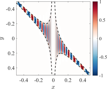
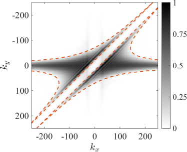
Figure 6: A snapshot of the vorticity field $\omega({\bf x},t)$ defined by Eq. (20) in the physical space for $s=20$, $h=0.1$, $\ell_{0}=1$, $Re=10^{7}$, and $\theta\approx 45^{\circ}$ (a). The black dashed line represents the boundary of the hyperbolic region given by inequality (49). The corresponding (normalized) power spectrum $\hat{H}(\mathbf{k})$ (b). The boundaries of the hyperbolic region defined by Eqs. (50) and (51) are shown as red dashed lines.

The enstrophy spectrum will also remain confined to a region of hyperbolic shape in Fourier space, with the “contracting” and “extending” directions making an angle $\theta$, as illustrated in Figure 6(b). The boundaries of this region are given by

$$\left|k_{x}k_{y}-\cot(\theta)k_{y}^{2}\right|\approx\frac{z(\bar{r})}{h^{2}}$$ (50)

and

$$\left|k_{x}-\cot(\theta)k_{y}\right|\approx\frac{\bar{r}}{\ell_{0}}.$$ (51)

The enstrophy spectrum in both the inertial and dissipation range changes rather insignificantly when the angle $\theta$ is varied. The most notable differences are at lower wavenumbers, as illustrated in Figure 7. In particular, the lower bound $k_{c}$ of the inertial range shifts towards higher wavenumbers when $\theta$ deviates increasingly from $90^{\circ}$. The shift of $k_{c}$ is due primarily to the spectral gap defined by Equation (51) progressively overlapping with the hyperbolic region near the $k_{x}$ axis.

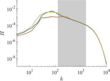
Figure 7: The enstrophy spectrum corresponding to the vorticity field (20) for different angles between the extending and contracting directions: $\theta=90^{\circ}$ (blue), $\theta=45^{\circ}$ (yellow) and $\theta=11.3^{\circ}$ (red). The gray background represents the inertial range for $\theta=90^{\circ}$.

5 Discussion

The useful analogy with chaotic advection of passive scalars (Kraichnan, 1971) yields substantial insight into the physical mechanisms of the direct cascade. Previous numerical simulations suggested that this analogy only holds in the hyperbolic regions of the flow (Lapeyre et al., 2001). The analysis presented in Section 3 shows that this analogy is much more nuanced. Specifically, we find the small-scale vorticity to behave as a passive scalar in regions where (i) vorticity of the large-scale flow is nearly constant and (ii) the curvature of the vorticity filaments representing small scales is low. In particular, even inside the hyperbolic regions, the sharp folds of the vorticity filaments are not simply advected by the large-scale flow ${\bf u}_{l}$; the small-scale flow ${\bf u}_{s}$ also plays an important role. On the other hand, we may find this analogy to hold inside the elliptic regions of the flow. For instance, large-scale vorticity inside vortex cores is often found to be relatively uniform – the flow field shown in Figure 2(a) represents an example of this – so that small-scale vorticity there satisfies the same evolution equation as in the hyperbolic regions and can also be considered a passive scalar.

The physical mechanism of the direct cascade described in this paper provides an explicit, quantitative relation between the properties of coherent structures and the scaling of enstrophy and energy in the inertial range. This mechanism refines the qualitative picture proposed by Kraichnan (1971) which involves stretching of filamentary vorticity in the straining regions of the large-scale flow. As shown here, the dynamics of vorticity filaments is described by a novel class of exact, self-similar (and hence scale-free) solutions of the Euler equation, naturally leading to a power-law scaling. Unlike the solutions of the Navier-Stokes equation describing coherent substructures (Deguchi, 2015; Eckhardt & Zammert, 2018; Yang et al., 2019; Doohan et al., 2019; Azimi & Schneider, 2020) or the solutions of the Euler equation describing large-scale coherent structures (Zhigunov & Grigoriev, 2022), the dynamically self-similar solutions reported here span the entire inertial range associated with the direct cascade. The relationship between different classes of solutions and the two cascades in high-$Re$ two-dimensional turbulence is summarized in Figure 8. It is worth emphasizing that, just as in the case of exact solutions of the Euler equation describing large-scale flows (Zhigunov & Grigoriev, 2022), dynamically self-similar solutions describing the direct cascade belong to families spanned by an infinite number of continuous parameters.

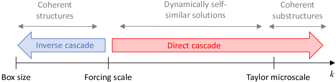
Figure 8: The relationship between the spatial scales, the cascades, and various classes of exact solutions of the governing equations in high-$Re$ two-dimensional turbulence.

Vortex thinning in the hyperbolic regions of the large-scale flow is exponentially fast. In contrast, the mechanism considered by Moffatt (1986) and Gilbert (1988) describes a relatively slow linear stretching of vorticity filaments in the vortical (elliptic) regions. Therefore, while both mechanisms operate at the same time, the former one plays the dominant role in the direct cascade and explains how power-law spectra can emerge on rather short time scales. Of course, the presence of these two mechanisms does not exclude other physical mechanisms that may contribute to the transport of enstrophy between scales. For instance, vorticity filaments can be stretched exponentially fast inside the vortex cores. Indeed, a time-dependent large-scale flow is generally expected to generate chaotic advection and global mixing in such circular geometries, provided various symmetries are broken (Grigoriev, 2005). We may also find exponential stretching of vorticity filaments at the edges of vortex cores, where the frequency of the time-dependent component of the flow is resonant with the frequency at which fluid elements are advected around the vortex by the time-independent component, as predicted by the KAM theory (Cartwright et al., 1999). Indeed, pronounced vortex filaments are found in these narrow regions as well, as illustrated by Figure 2(a).

Time-dependence of the large-scale flow, which has not been fully appreciated previously, also plays a critical role in vortex thinning in the hyperbolic regions. Chaotic advection generally requires both stretching and folding. While stretching is generic in any flow with nontrivial structure, folding is a direct result of time-dependence. It should be emphasized that the mechanism described by Moffatt (1986) and Gilbert (1988) involves no time-dependence and hence no folding. In the hyperbolic regions, the structure of vorticity filaments, and the associated Fourier spectrum, is crucially impacted by both the time-dependent and time-independent component of the large-scale flow. In particular, the ratio $s$ of the associated time scales introduced here, strongly affects the small-scale structures that emerge and hence the scaling of the energy and enstrophy. Note that while the turbulent flow considered here is not time-periodic on long time scales, it is found to be nearly time-periodic on short time scales (Zhigunov & Grigoriev, 2022). Since the stretching of filaments is exponentially fast, the large-scale flow can be considered time-periodic with a slow drift in $s$ reflected in the variation of the exponent $\alpha$ shown in Figure 1(b).

The KLB theory crucially relies on the assumption that stretching of small-scale vorticity patches in different hyperbolic regions is uncorrelated. Deviations from the KLB predictions are expected whenever this assumption breaks down. Indeed, for the numerical simulations of turbulence considered here, the large-scale flow, a representative snapshot of which is shown in Figure 2, has two hyperbolic regions. The dynamics in the two hyperbolic regions are strongly correlated. In particular, the stretching (contracting) direction in one hyperbolic region is well-aligned with the contracting (stretching) direction in the other. In order to understand and describe the non-universal aspects of the direct cascade and, in particular, determine the enstrophy/energy scaling in the inertial range, these correlations imposed by the large-scale flow have to be understood and properly quantified.

Each of the two saddle points of the large-scale flow has an associated stable and unstable manifold whose directions coincide, near the saddle, with the contracting and extending direction of the flow. When the large-scale flow is time-periodic, the unstable manifold of one saddle crosses the stable manifold of the other, forming a heteroclinic tangle (Ottino, 1990), as illustrated in Figure 9(a). Since the large-scale flow acts to align vorticity filaments in each hyperbolic region along the corresponding unstable manifold, this tangle is what controls the shape and orientation of the filaments. When the filaments leave one hyperbolic region, they enter the other, and the angle at which the unstable manifold of one saddle intersect the stable manifold of the other depends on the amplitude of the time-dependent component of the large-scale flow. As illustrated in Figure 9(b), the relative orientation of the manifolds also affects the structure of the vorticity field at the entrance to each hyperbolic region and hence determines whether the small-scale vorticity inside each hyperbolic region is described by either of the two self-similar solutions $g_{c}^{\pm}(\xi)$ and $g_{e}^{\pm}(\eta)$ introduced in Section 3 or the general solution (7) that depends on both similarity variables. For time-periodic large-scale flows, the heteroclinic tangle also controls the shape and thickness $h$ of the hyperbolic regions, substantially simplifying the analysis compared to the aperiodic case where even separating the flow domain into elliptic and hyperbolic regions is not straightforward (Haller, 2001).

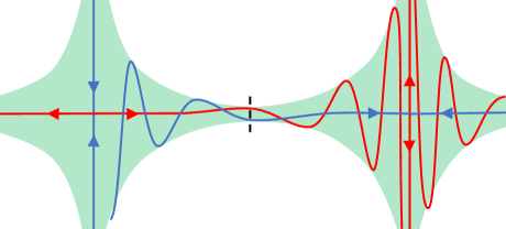
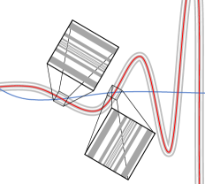
Figure 9: Vorticity transport in hyperbolic regions (shown in green) of a time-periodic large-scale flow. (a) Unstable manifolds (red) of a saddle tangling with the stable manifold (blue) of an adjacent saddle. The dashed line shows the boundary between the hyperbolic regions. (b) Small-scale structure of the vorticity field with vorticity filaments (grayscale) locally aligned along the unstable manifold.

The presence of small-scale structure at the entrance to a hyperbolic region could in itself have a significant impact on the enstrophy/energy scaling and requires further study. The results presented in Section 4.2 illustrate one way in which the scaling $H(k)\propto k^{-1}$ might break down when the vorticity field at the entrance to a hyperbolic region contains multiple scales. The left boundary of the inertial range is predicted to scale as $k_{c}=k_{s}\propto ns$ in the limit of $ns$-large. When the Fourier series (10) includes contributions with high $n$, one may find $k_{c}>k_{d}$, so that our prediction (40) becomes inaccurate for all $k$, leading to a different scaling (or at least a different scaling exponent).

Furthermore, as Figure 2 shows, at the entrances to both hyperbolic regions, vorticity field has a lot of small-scale structure with vorticity filaments preferentially aligned along the contracting direction of the large-scale flow. The dynamics of vorticity filaments with such orientation is described by the self-similar solution $g_{e}^{\pm}(\eta)$ representing the flux of enstrophy towards large, rather than small, scales. Proper quantitative description of this phenomenon known as backscatter is crucial for subgrid-scale modeling. However, correlations induced by the large-scale flow are accounted for neither in the KLB theory nor in the stochastic approaches to modeling eddy viscosity (Kraichnan, 1976; Leslie & Quarini, 1979; Leith, 1990). Backscatter amplifies the large scales at the expense of the small scales and should therefore, make the spectra of enstrophy and energy steeper, in perfect agreement with the results of our numerical simulations shown in Figure 1. It is worth emphasizing that enstrophy flows in both directions at all times, with the flux towards small (large) scales in regions where small-scale vorticity filaments are preferentially aligned along the extending (contracting) direction of the large-scale flow. Backscatter, and consequently the energy/enstrophy scaling in the inertial range, are non-universal and cannot be expected to be described properly by statistical descriptions agnostic of coherent structures.

6 Conclusion

We introduced here a mechanistic, dynamical description of the vortex thinning mechanism which explains when the classical KLB theory of the direct cascade in two-dimensional turbulence applies and when and why it fails. This description crucially relies on two classes of solutions of the Euler equation: (weakly unstable) time-periodic solutions describing the “large” scales (i.e., scales comparable to the system size) and self-similar solutions describing the “small” scales or, more specifically, a wide range of scales representing the inertial range. The self-similar, i.e., scale-free, nature of the latter class of solutions is the fundamental reason why power-law scaling of energy and enstrophy is found in the inertial range, regardless of whether the scaling exponent is integer or fractal.

Our dynamical description not only reproduces the predictions of the KLB theory for the energy/enstrophy scaling in the inertial range, but also predicts the scaling in the dissipation range. The inertial range scaling $E(k)\propto k^{-3}$ (or, equivalently, $H(k)\propto k^{-1}$) predicted by the KLB theory reflects the universal aspect of two-dimensional turbulence: exponentially fast stretching of small-scale vorticity filaments as they are advected by the large-scale flow inside the hyperbolic regions of that flow. What the KLB theory fails to describe is the correlations between adjacent hyperbolic regions associated with the structure of the large-scale flow, i.e., the presence of coherent structures, which lead to varying degrees of backscatter (enstrophy flux from small to large scales).

In the absence of correlations between adjacent hyperbolic regions, the enstrophy/energy spectra are found to have a universal scaling exponent in the inertial range. However, the wavenumber range over which this scaling is found is not universal. Its high-wavenumber boundary depends on the Reynolds number, while the low-wavenumber boundary depends on the properties of the large-scale flow, i.e., the characteristic size and width of the hyperbolic regions as well as the ratio of the strain rate $\mathcal{E}$ of the time-independent component of the flow and the characteristic temporal frequency $\Omega$ of the time-dependent component. Similarly, the scaling in the dissipative range is found to be non-universal and to depend on this ratio.

This study does not provide an explicit relation between the properties of coherent structures (i.e., the spatial and temporal structure of the large-scale flow) and the spectrum of the enstrophy and energy generated in the inertial range by the direct cascade. However, it makes explicit the limitations of the KLB theory and paves the way for a more general description of the direct cascade that would explain this relation and would be capable of predicting the spectra based on the properties of coherent structures. Even without such a detailed description, it becomes apparent that fractal scaling exponents observed in experiments and numerical simulations based on the Navier-Stokes equation are due to the emergence of fractal filamentary structures generated by chaotic advection of small-scale vorticity through connected hyperbolic regions of the large-scale flow.

Acknowledgements. This material is based upon work supported by the National Science Foundation under grant no. 2032657.

Declaration of interests. The authors report no conflict of interest.

References

- Aref et al. (2003) Aref, Hassan, Newton, Paul K, Stremler, Mark A, Tokieda, Tadashi & Vainchtein, Dmitri L 2003 Vortex crystals. Advances in applied Mechanics 39, 2–81.
- Azimi & Schneider (2020) Azimi, Sajjad & Schneider, Tobias M 2020 Self-similar invariant solution in the near-wall region of a turbulent boundary layer at asymptotically high reynolds numbers. Journal of Fluid Mechanics 888.
- Batchelor (1969) Batchelor, George K 1969 Computation of the energy spectrum in homogeneous two-dimensional turbulence. The Physics of Fluids 12 (12), II–233.
- Benzi et al. (1988) Benzi, R, Patarnello, S & Santangelo, P 1988 Self-similar coherent structures in two-dimensional decaying turbulence. Journal of Physics A: Mathematical and General 21 (5), 1221.
- Boffetta & Ecke (2012) Boffetta, Guido & Ecke, Robert E 2012 Two-dimensional turbulence. Annual Review of Fluid Mechanics 44, 427–451.
- Borue (1993) Borue, Vadim 1993 Spectral exponents of enstrophy cascade in stationary two-dimensional homogeneous turbulence. Physical review letters 71 (24), 3967.
- Bracco et al. (2000) Bracco, A., McWilliams, J. C., Murante, G., Provenzale, A. & Weiss, J. B. 2000 Revisiting freely decaying two-dimensional turbulence at millennial resolution. Physics of Fluids 12 (11), 2931–2941, arXiv: https://pubs.aip.org/aip/pof/article-pdf/12/11/2931/12525238/2931_1_online.pdf.
- Brachet et al. (1987) Brachet, ME, Meneguzzi, M, Politano, H & Sulem, PL 1987 Computer simulation of decaying two-dimensional turbulence. In Advances in Turbulence, pp. 245–254. Springer.
- Cartwright et al. (1999) Cartwright, Julyan HE, Feingold, Mario & Piro, Oreste 1999 An introduction to chaotic advection. Mixing: Chaos and turbulence pp. 307–342.
- Chen et al. (2003) Chen, Shiyi, Ecke, Robert E, Eyink, Gregory L, Wang, Xin & Xiao, Zuoli 2003 Physical mechanism of the two-dimensional enstrophy cascade. Physical review letters 91 (21), 214501.
- Chertkov et al. (2007) Chertkov, M, Connaughton, C, Kolokolov, I & Lebedev, V 2007 Dynamics of energy condensation in two-dimensional turbulence. Physical review letters 99 (8), 084501.
- Clercx & Van Heijst (2009) Clercx, HJH & Van Heijst, GJF 2009 Two-dimensional navier–stokes turbulence in bounded domains. Applied Mechanics Reviews 62 (2).
- Deguchi (2015) Deguchi, Kengo 2015 Self-sustained states at kolmogorov microscale. Journal of Fluid Mechanics 781.
- Doohan et al. (2019) Doohan, Patrick, Willis, Ashley P. & Hwang, Yongyun 2019 Shear stress-driven flow: the state space of near-wall turbulence as . Journal of Fluid Mechanics 874, 606–638.
- Eckhardt & Zammert (2018) Eckhardt, Bruno & Zammert, Stefan 2018 Small scale exact coherent structures at large Reynolds numbers in plane Couette flow. Nonlinearity 31 (2), R66.
- Gilbert (1988) Gilbert, Andrew D 1988 Spiral structures and spectra in two-dimensional turbulence. Journal of Fluid Mechanics 193, 475–497.
- Grigoriev (2005) Grigoriev, Roman O 2005 Chaotic mixing in thermocapillary-driven microdroplets. Physics of fluids 17 (3), 033601.
- Haller (2001) Haller, George 2001 Lagrangian structures and the rate of strain in a partition of two-dimensional turbulence. Physics of Fluids 13 (11), 3365–3385.
- Herring & McWilliams (1985) Herring, JR & McWilliams, JC 1985 Comparison of direct numerical simulation of two-dimensional turbulence with two-point closure: the effects of intermittency. Journal of Fluid Mechanics 153, 229–242.
- Kelley & Ouellette (2011) Kelley, Douglas H & Ouellette, Nicholas T 2011 Spatiotemporal persistence of spectral fluxes in two-dimensional weak turbulence. Physics of Fluids 23 (11), 115101.
- Kim et al. (2017) Kim, Sun-Chul, Miyaji, Tomoyuki & Okamoto, Hisashi 2017 Unimodal patterns appearing in the two-dimensional navier–stokes flows under general forcing at large reynolds numbers. European Journal of Mechanics - B/Fluids 65, 234–246.
- Kim & Okamoto (2010) Kim, Sun-Chul & Okamoto, Hisashi 2010 Vortices of large scale appearing in the 2d stationary navier–stokes equations at large reynolds numbers. Japan Journal of Industrial and Applied Mathematics 27 (1), 47–71.
- Kim & Okamoto (2015) Kim, Sun-Chul & Okamoto, Hisashi 2015 Unimodal patterns appearing in the kolmogorov flows at large reynolds numbers. Nonlinearity 28 (9), 3219.
- Kraichnan (1967) Kraichnan, Robert H 1967 Inertial ranges in two-dimensional turbulence. The Physics of Fluids 10 (7), 1417–1423.
- Kraichnan (1971) Kraichnan, Robert H. 1971 Inertial-range transfer in two- and three-dimensional turbulence. Journal of Fluid Mechanics 47 (3), 525–535.
- Kraichnan (1976) Kraichnan, Robert H 1976 Eddy viscosity in two and three dimensions. Journal of Atmospheric Sciences 33 (8), 1521–1536.
- Lapeyre et al. (2001) Lapeyre, G, Hua, BL & Klein, P 2001 Dynamics of the orientation of active and passive scalars in two-dimensional turbulence. Physics of Fluids 13 (1), 251–264.
- Lapeyre et al. (1999) Lapeyre, G, Klein, P & Hua, BL 1999 Does the tracer gradient vector align with the strain eigenvectors in 2d turbulence? Physics of fluids 11 (12), 3729–3737.
- Legras et al. (1988) Legras, B, Santangelo, P & Benzi, R 1988 High-resolution numerical experiments for forced two-dimensional turbulence. EPL (Europhysics Letters) 5 (1), 37.
- Leith (1990) Leith, CE 1990 Stochastic backscatter in a subgrid-scale model: Plane shear mixing layer. Physics of Fluids A: Fluid Dynamics 2 (3), 297–299.
- Leith (1968) Leith, Cecil E 1968 Diffusion approximation for two-dimensional turbulence. The Physics of Fluids 11 (3), 671–672.
- Leslie & Quarini (1979) Leslie, DC & Quarini, GL 1979 The application of turbulence theory to the formulation of subgrid modelling procedures. Journal of fluid mechanics 91 (1), 65–91.
- Liao & Ouellette (2015) Liao, Yang & Ouellette, Nicholas T 2015 Correlations between the instantaneous velocity gradient and the evolution of scale-to-scale fluxes in two-dimensional flow. Physical Review E 92 (3), 033017.
- Maltrud & Vallis (1991) Maltrud, ME & Vallis, GK 1991 Energy spectra and coherent structures in forced two-dimensional and beta-plane turbulence. Journal of Fluid Mechanics 228, 321–342.
- McWilliams (1984) McWilliams, James C 1984 The emergence of isolated coherent vortices in turbulent flow. Journal of Fluid Mechanics 146, 21–43.
- Moffatt (1986) Moffatt, HK 1986 Advances in turbulence. Springer-Verlag, Berlin 284, 284.
- Ottino (1990) Ottino, Julio M 1990 Mixing, chaotic advection, and turbulence. Annual Review of Fluid Mechanics 22 (1), 207–254.
- Rivera et al. (2014) Rivera, MK, Aluie, Hussein & Ecke, RE 2014 The direct enstrophy cascade of two-dimensional soap film flows. Physics of Fluids 26 (5), 055105.
- Saffman (1971) Saffman, PG 1971 On the spectrum and decay of random two-dimensional vorticity distributions at large reynolds number. Studies in Applied Mathematics 50 (4), 377–383.
- Smith & Yakhot (1994) Smith, Leslie M & Yakhot, Victor 1994 Finite-size effects in forced two-dimensional turbulence. Journal of Fluid Mechanics 274, 115–138.
- Yang et al. (2019) Yang, Qiang, Willis, Ashley P & Hwang, Yongyun 2019 Exact coherent states of attached eddies in channel flow. Journal of Fluid Mechanics 862, 1029–1059.
- Zhigunov & Grigoriev (2022) Zhigunov, Dmitriy & Grigoriev, Roman O. 2022 Exact coherent structures in fully developed two-dimensional turbulence.