The effect of Quantum Statistics on the sensitivity in an SU(1,1) interferometer

Abstract

We theoretically study the effect of quantum statistics of the light field on the quantum enhancement of parameter estimation based on cat state input the SU(1,1) interferometer. The phase sensitivity is dependent on the relative phase $\theta$ between two coherent states of Schrödinger cat states. The optimal sensitivity is achieved when the relative phase is $\pi$, i.e., odd coherent states input. For a coherent state input into one port, the phase sensitivity of the odd coherent state into the second input port is inferior to that of the squeezed vacuum state input. However, in the presence of losses the Schrödinger cat states are more resistant to loss than squeezed vacuum states. As the amplitude of Schrödinger cat states increases, the quantum enhancement of phase sensitivity decreases, which shows that the quantum statistics of Schrödinger cat states tends towards Poisson statistics from sub-Poisson statistics or super-Poisson statistics.

I Introduction

In quantum metrology, the Mach–Zehnder interferometer (MZI) and its variant SU(1,1) interferometer Yurke86 had been used as a generic model to realize precise measurement of phase. Using quantum measurement techniques to beat the standard quantum limit (SQL) has received a lot of attention in recent years Helstrom67 ; Holevo82 ; Caves81 ; Braunstein94 ; Braunstein96 ; Lee02 ; Giovannetti06 ; Zwierz10 ; Giovannetti04 ; Giovannetti11 ; Hudelist14 . By optimizing over all possible estimators, measurements, and probe states the accuracy of parameter estimation can be improved. Forty years ago, Caves Caves81 suggested to replace the vacuum fluctuations with the squeezed-vacuum light in the MZI to reach a sub-shot-noise sensitivity. Soon after, various quantum resources were used to improve the measurement precision Xiao ; Grangier ; Dowling08 ; N00N . Due to the even coherent states also are superposition of even number states, they are closely related to the squeezed vacuum states, but with different coefficients. The even and odd coherent states is called also Schrödinger cat states and is written as $|cat\rangle=(|\alpha\rangle+e^{i\theta}|-\alpha\rangle)/\sqrt{N}$ with $N=2+2e^{-2\alpha^{2}}cos\theta$ is the normalization factor and $\theta$ is the relative phase, where $\theta=0$, $\pi$, and $\pi/2$ corresponds to the even coherent states, odd coherent states, and Yurke-Stoler states Gerry05 . The even and odd coherent states have been predicted in interferometric detection of gravitation waves for reducing the optimal intensity of the input laser Ansari . The photon statistics of single-mode and multimode even and odd coherent states are also studied Buzik92 ; Ansari94 . The use of non-classical states can enhance the accuracy of parameter estimation, which comes from the quantum statistics of non-classical states: super-Poissonian statistics or sub-Poissonian statistics. Given a constraint on the amplitude of Schrödinger cat state, analyzing the quantum enhancement of the parameter estimation by changing the quantum statistics of the cat state is worth studying to further explain the origin of the quantum enhancement of the phase parameter estimation. On the other hand, the measurement precision of interferometers will be reduced in the presence of environment noise Escher ; Dem12 ; Dem09 . For interferometers, the photon losses is a typical decoherence process to be taken into account. Analyzing and studying the influence of photon loss on the sensitivity of the cat state, and comparing the result with that of the squeezed vacuum state is very helpful for the application of the cat state in quantum metrology.

Quantum parameter estimation theory establishes the ultimate lower bound to the sensitivity with which a classical parameter (e.g., phase shift $\phi$) that parameterizes the quantum state can be measured. The popular way to obtain the lower bounds in quantum metrology, is to use the method of the quantum Fisher information (QFI) Braunstein94 ; Braunstein96 . It establishes the best precision that can be attained with a given quantum probe. In recent years, to obtain the QFI many efforts have been made by theory Toth ; PezzBook ; Demkowicz ; Wang ; Jarzyna ; Monras ; Pinel ; Liu ; Gao ; Jiang ; Safranek ; Sparaciari15 ; Sparaciari and experiments Strobel ; Hauke . Since interferometers as a generic model to realize precise estimation of phase shift, the corresponding QFI has been studied. For the MZI, Jarzyna et al. Jarzyna studied the QFIs between phase shifts in the single arm case and in the two-arm case and presented the differences between them. Many measurement processes do not include phase reference, and the conclusions of QFI-only calculations will be overestimated, which cannot be realized at all via exact inputs and measurements Jarzyna ; Takeoka ; Zhong ; Zhang . For phase shifts in the two-arm case, the phase estimation can be considered as a two parameter estimation problem. In general, the calculation of the quantum Fisher information matrix (QFIM) is necessary Lang1 ; Lang2 ; Ataman ; You19 ; Zhong2 .

In this paper, we study the cat state injection SU(1,1) interferometer and analyze the relationship between photon statistics and phase sensitivity. To avoid overestimation from QFI-only calculation, the conclusive quantum Craḿer-Rao bound (QCRB) based on the QFIM approach is derived. The sensitivity of the optimized cat state input and the squeezed vacuum state input are compared and studied, as well as the loss-resistant behavior in the presence of losses.

II Phase sensitivity

II.1 QFI and Mandel Q-parameter

An SU(1,1) interferometer is considered, as shown in Fig. 1, where the nonlinear beam splitters (NBSs) can be realized by the optical parametric amplifiers (OPAs) or four-wave mixing (FWM) Jing11 ; Chen15 . In the Heisenberg picture the transformation of the mode operators is

$$\hat{a}=u\hat{a}_{0}+v\hat{b}_{0}^{\dagger},\text{ \ }\hat{b}^{\dagger}=u^{\ast}\hat{b}_{0}^{\dagger}+v^{\ast}\hat{a}_{0},$$ (1)

where $u=\cosh g$, and $v=e^{i\theta_{g}}\sinh g$. After the light field passing the first NBS, as shown in Fig. 1, the two beams sustain phase shifts, i.e., mode $a$ undergoes a phase shift of $\phi_{a}$ and mode $b$ undergoes a phase shift of $\phi_{b}$. The transformation of phase shift is described as

$$\hat{U}_{\phi}^{ab}=\exp[i\phi_{a}\hat{n}_{a}+i\phi_{b}\hat{n}_{b}]=\exp(i\phi_{s}\hat{g}_{s})\exp(i\phi_{d}\hat{g}_{d}),$$ (2)

where $\hat{n}_{a}=\hat{a}^{\dagger}\hat{a}$, $\hat{n}_{b}=\hat{b}^{\dagger}\hat{b}$, $\phi_{s,d}=\phi_{a}\pm\phi_{b}$ and $g_{s,d}=(\hat{n}_{a}\pm\hat{n}_{b})/2$. In the SU(1,1) interferometer the quantity to estimate is the phase sum $\phi_{s}$ Kok10 .

In general, the phase estimation as a two-parameter estimation problem, the QFIM approach is necessary. For the estimation of $\phi_{s}$ and $\phi_{d}$ we can use the method of QFIM, which is given by a two-by-two matrix

$$\mathcal{F}=\left[\begin{array}[]{cc}F_{ss}&F_{sd}\\ F_{ds}&F_{dd}\end{array}\right],$$ (3)

where $F_{ij}=4(\langle\psi_{\phi}|\hat{g}_{i}\hat{g}_{j}|\psi_{\phi}\rangle-\langle\psi_{\phi}|\hat{g}_{i}|\psi_{\phi}\rangle\langle\psi_{\phi}|\hat{g}_{j}|\psi_{\phi}\rangle)$ ($i,j=s,d$). In the SU(1,1) interferometer, we are usually interested in the estimation of only $\phi_{s}$ and its corresponding QFI is given by

$$\mathcal{F}=\frac{1}{\Delta^{2}\phi_{s}}=F_{ss}-\frac{F_{sd}F_{ds}}{F_{dd}}.$$ (4)

After calculation, the $\mathcal{F}$ is worked as

$$\mathcal{F}=4\frac{\langle\Delta^{2}\hat{n}_{a}\rangle\langle\Delta^{2}\hat{n}_{b}\rangle-Cov[n_{a},n_{b}]^{2}}{\langle\Delta^{2}\hat{n}_{a}\rangle+\langle\Delta^{2}\hat{n}_{b}\rangle-2Cov[n_{a},n_{b}]},$$ (5)

where $\langle\Delta^{2}\hat{n}_{i}\rangle=\langle\hat{n}_{i}^{2}\rangle-\langle\hat{n}_{i}\rangle^{2}$ ($i=a,b$), $Cov[n_{a},n_{b}]=\langle\hat{n}_{a}\hat{n}_{b}\rangle-\langle\hat{n}_{a}\rangle\langle\hat{n}_{b}\rangle$, $\langle\cdot\rangle$ denotes the average value $\left\langle\psi\right|\cdot|\psi\rangle$, and $|\psi\rangle$ is the state of probe state $|\psi_{in}\rangle$ after being prepared by a NBS. We use the Mandel $Q$-parameter to describe the photon statistics of state $|\psi\rangle$, which is given by

$$Q_{i}=\frac{\left\langle\hat{n}_{i}^{2}\right\rangle-\langle\hat{n}_{i}\rangle^{2}}{\langle\hat{n}_{i}\rangle}-1\text{ }(i=a,b),$$ (6)

where $\langle\Delta\hat{n}_{i}\rangle=\sqrt{\langle\Delta^{2}\hat{n}_{i}\rangle}$. Using the Mandel $Q$-parameter, the $\mathcal{F}$ is rewritten as

$$\mathcal{F}=\frac{4(\left\langle\hat{n}_{a}\right\rangle\left\langle\hat{n}_{b}\right\rangle(Q_{a}+1)(Q_{b}+1)-Cov[\hat{n}_{a},\hat{n}_{b}]^{2})}{\left\langle\hat{n}_{b}\right\rangle(Q_{b}+1)+\left\langle\hat{n}_{a}\right\rangle(Q_{a}+1)-2Cov[\hat{n}_{a},\hat{n}_{b}]}.\text{ }\text{ }$$ (7)

Note that $Q_{a,b}$ here describes the Mandel $Q$-value of the light field in the two arms of the interferometer.

The above inequality shows that the metrological advantage of nonclassical light is primarily the photon statistics Mandel parameters $Q_{a}$ and $Q_{b}$ in the two arms of interferometer, and convariance $Cov[\hat{n}_{a},\hat{n}_{b}]$. Next, we study the effect of quantum statistics of input fields on the sensitivity in an SU(1,1) interferometer.

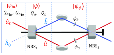
Figure 1: Schematic of an SU(1,1) interferometer. $|\psi_{in}\rangle$: initial state; $|\psi\rangle$: probe preparation; $|\psi_{\phi}\rangle$: state after phase encoding. $\phi_{a}$, $\phi_{b}$: phase shift; $\mathrm{NBS}_{1,2}$: nonlinear beam splitter; $Q_{a_{in},b_{in}}$, and $Q_{a,b}$ are the Mandel Q-parameters of the input light fields and the light fields of the two arms inside the interferometer, respectively.

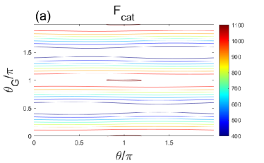
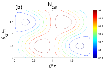
Figure 2: Schrödinger cat state and coherent state input. (a) QFI $F_{cat}$ and (b) total number of photons $N_{cat}$ inside the interferometer as a function of $\theta$ and $\theta_{G}$, where $g=1.2$, $\alpha=1.2$, and $\beta_{G}=1.8$.

II.2 QFI of Schrödinger cat state and coherent state

We analysis for the input of Schrödinger cat state $|cat\rangle=(|\alpha\rangle+e^{i\theta}|-\alpha\rangle)/\sqrt{N}$ with $N=2+2e^{-2\alpha^{2}}cos\theta$ in mode $a$ and coherent state $|\beta\rangle$ ($\beta=\left|\beta\right|e^{i\theta_{\beta}}$) in mode $b$. By using the QFIM method, we have

$$\mathcal{F}_{\mathrm{cat}} = \sinh^{2}(2g)[\bar{n}_{\alpha}+(1+2\bar{n}_{\alpha})\left|\beta\right|^{2}+1]$$

$$+ 4\cosh^{2}(2g)\left|\beta\right|^{2}+4\cosh(2g)\bar{n}_{q}+4(\bar{n}_{Q}-\bar{n}_{q}^{2})$$

$$- 4\frac{[\cosh(2g)\left|\beta\right|^{2}+(\alpha^{2}+\bar{n}_{\alpha})\bar{n}_{q}]^{2}}{\alpha^{4}+\bar{n}_{\alpha}-\bar{n}_{\alpha}^{2}+\left|\beta\right|^{2}},$$ (8)

with

$$\bar{n}_{q} = (e^{-2|\alpha|^{2}}\sin\theta/z_{s})\sinh(2g)\alpha\left|\beta\right|\sin(\theta_{G}),$$

$$\bar{n}_{Q} = \frac{1}{2}\sinh^{2}(2g)\alpha^{2}\left|\beta\right|^{2}\cos(2\theta_{G}),$$ (9)

where $\theta_{G}=\theta_{\beta}-\theta_{g}$, $\bar{n}_{\alpha}=\langle cat|\hat{a}_{0}^{{\dagger}}\hat{a}_{0}|cat\rangle=\alpha^{2}(z_{d}/z_{s})$ with $z_{s,d}=1\pm e^{-2\alpha^{2}}cos\theta$, $\bar{n}_{\alpha}$ is the average photon number of cat state. Based on the QFI, the ultimate precision bound of phase sensitivity is given by the QCRB

$$\Delta\phi_{\mathrm{QCRB}}=\frac{1}{\sqrt{m\mathcal{F}}},$$ (10)

where $m$ is the number of independent repeats of the experience.

When $\beta=0$, i. e., $|cat\rangle_{a}\otimes|0\rangle_{b}$ input, $\mathcal{F}_{\mathrm{cat}}$ is reduced to QFI of Schrödinger cat state and vacuum state

$$\mathcal{F}_{\mathrm{cat}}=\sinh^{2}(2g)(1+\bar{n}_{\alpha}).$$ (11)

The QFI of above Eq. (11) is dependent on the average photon number of cat state $\bar{n}_{\alpha}$. For a given amplitude $\alpha$ of Schrödinger cat state, when the relative phases $\theta$ is changed, the average number of photon $\bar{n}_{\alpha}$ is also changed. When $\theta=0$, $\pi$, and $\pi/2$, $\bar{n}_{\alpha}$ corresponds to $\alpha^{2}\frac{1-e^{-2\alpha^{2}}}{1+e^{-2\alpha^{2}}}<\alpha^{2}$, $\alpha^{2}\frac{1+e^{-2\alpha^{2}}}{1-e^{-2\alpha^{2}}}>\alpha^{2}$, and $\alpha^{2}$. When $\theta=(2k+1)\pi$ ($k=0,1,2,\cdots$), the maximal $\bar{n}_{\alpha}$ is obtained for a given $\alpha$. When $\beta\neq 0$, for a given $\alpha$ and $|\beta|$, the QFI $\mathcal{F}_{\mathrm{cat}}$ as a function of $\theta$ and $\theta_{G}$ is shown in Fig. 2(a). The maximum value of QFI $\mathcal{F}_{\mathrm{cat}}$ occurs at $\theta=(2k+1)\pi$ and $\theta_{G}=k\pi$ ($k=0,1,2,\cdots$). Thus, the optimal sensitivity is achieved when odd coherent state input.

The quantum enhancement of phase sensitivity can be explained by the Mandel $Q$-parameter of input fields. The $Q$-parameter for the even coherent states is $Q_{a_{in}}=4\alpha^{2}e^{-\alpha^{2}}/(1+e^{-4\alpha^{2}})>0$ indicating super-Poissonian statistics, and for the odd coherent states is $Q_{a_{in}}=4\alpha^{2}e^{-\alpha^{2}}/(1+e^{-4\alpha^{2}})<0$ indicating sub-Poissonian statistics, and for Yurke-Stoler states is $Q_{a_{in}}=0$. Since the odd coherent state input can obtain the optimal phase sensitivity, that is, the input field with sub-Poisson statistics $(Q_{a_{in}}<0)$ can obtain the best sensitivity for phase measurement, which is opposite to the $Q_{a}$ and $Q_{b}$ value of the light field of the two arms inside the interferometer.

As $\alpha$ becomes large, $Q_{a_{in}}$ $\rightarrow 0$, which shows the effect of Schrödinger cat states is equivalent to coherent state. The enhancement of phase sensitivity due to quantum statistics gradually decreases to $0$ as $\alpha$ increases.

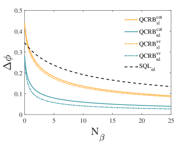
Figure 3: Phase sensitivity versus the photon number $N_{\beta}$ with the two input states $\left|cat\right\rangle_{a}\otimes\left|\beta\right\rangle_{b}$ and $\left|\xi\right\rangle_{a}\otimes\left|\beta\right\rangle_{b}$ and average photon number $\bar{n}_{\alpha}=\bar{n}_{s}$, $\alpha=2$, $g=1.2$, $\eta_{a}=0.5$, $\eta_{b}=1$, $\theta=\pi$ and $\theta_{G}=\pi$. QCRB${}_{p}^{k}$: $k\in$[cat, $\left|cat\right\rangle_{a}\otimes\left|\beta\right\rangle_{b}$ case; sv, $\left|\xi\right\rangle_{a}\otimes\left|\beta\right\rangle_{b}$ case], $p\in$[sl, single arm loss case; nl, lossless case]. The black dotted line is the SQL in the lossless case.

III Comparison between cat state and Squeezed state

It is also worthwhile to compare the above result with that of squeezed vacuum $|0,\xi\rangle$ $(\xi=re^{i\eta}$) in mode $a$ and coherent state in mode $b$, where $r$ is the squeezing strength of the squeezed vacuum, and its QFI is as follows You19 :

$$\mathcal{F}_{{}_{\mathrm{sv}}} = \sinh^{2}(2g)[\left|\beta\right|^{2}e^{2r}+\cosh^{2}(r)]$$ (12)

$$+\cosh^{2}(2g)\frac{8\left|\beta\right|^{2}\sinh^{2}(2r)}{4\left|\beta\right|^{2}+2\sinh^{2}(2r)}.$$

When $\beta=0$, $\mathcal{F}_{\mathrm{sv}}$ is reduced to

$$\mathcal{F}_{\mathrm{sv}}=\sinh^{2}(2g)[1+\bar{n}_{s}],$$ (13)

where $\bar{n}_{s}=\sinh^{2}r$, $\bar{n}_{s}$ is the average photon number of the squeezed vacuum state. Comparing Eq. (11) with Eq. (13), their QFIs are equal when $\bar{n}_{\alpha}=$ $\bar{n}_{s}$.

The total number of photons $\langle\hat{N}\rangle$ inside the SU(1,1) interferometer is given by $\langle\hat{N}\rangle\equiv\langle\hat{a}^{{\dagger}}\hat{a}\rangle+\langle\hat{b}^{{\dagger}}\hat{b}\rangle$. For input state $|0,\xi\rangle_{a}\otimes|\beta\rangle_{b}$ and $|cat\rangle_{a}\otimes|\beta\rangle_{b}$, their total number of photons $N_{\mathrm{sv}}$ and $N_{\mathrm{cat}}$ are respectively as follows:

$$N_{\mathrm{sv}} = \cosh(2g)(\left|\beta\right|^{2}+\bar{n}_{s})+2\sinh^{2}g,$$ (14)

$$N_{\mathrm{cat}} = \cosh(2g)(\left|\beta\right|^{2}+\bar{n}_{\alpha})+2\sinh^{2}g+2\bar{n}_{q},$$ (15)

where the first term on the right-hand side, $\cosh(2g)(\left|\beta\right|^{2}+\bar{n}_{s})$ or $\cosh(2g)(\left|\beta\right|^{2}+\bar{n}_{\alpha})$, results from the amplification process of the input photon number and the second one $2\sinh^{2}g$ corresponds to amplification of the vacuum input state or the so-called spontaneous process. The expression $N_{\mathrm{cat}}$ has an additional term, $2\bar{n}_{q}$, which is due to the intensity correlation of the two input fields. When odd coherent state input [$\theta=(2k+1)\pi$ ($k=0,1,2,\cdots$)], $\bar{n}_{q}$ equals 0.

Fig. 2(b) shows the contour lines of $N_{\mathrm{cat}}$ as a function of $\theta$ and $\theta_{G}$. The maximum value of $N_{\mathrm{cat}}$ occurs in two regions that are symmetric about $\theta=\theta_{G}=\pi$. The parameters corresponding to the maximum value of the phase-sensitive photon number and QFI are different, because QFI depends more on the fluctuation and statistical properties of the input light field.

For a given $\alpha$ ($\bar{n}_{\alpha}=\bar{n}_{s}$) and $\theta_{G}=\theta=\pi$, the sensitivity of $|0,\xi\rangle_{a}\otimes|\beta\rangle_{b}$ and $|cat\rangle_{a}\otimes|\beta\rangle_{b}$ input is compared in Fig. 3, which agrees with the result given by Lang and Caves Lang1 . That is, for a coherent state input into one port, the best state to inject into the second input port is the squeezed vacuum state.

IV Losses

In this section, we investigate the effects of losses on the phase sensitivity. We use the extended model Zeng23 to calculate the QFIMs in the presence of losses in one arm and losses in two arms.

For the enlarged system-environment state, the QFI $\mathcal{C}_{\mathrm{cat}}$ is given by

$$\mathcal{C}=\left[\begin{array}[]{cc}C_{ss}&C_{sd}\\ C_{ds}&C_{dd}\end{array}\right],$$ (16)

where

$$C_{ij} = 4[\left\langle\psi\right|_{S}\left\langle l\right|_{E}\sum_{l\mathrm{cat}}\frac{d\hat{\Pi}_{l}^{{\dagger}}(x_{s},x_{d})}{d\phi_{i}}\frac{d\hat{\Pi}_{l}(x_{s},x_{d})}{d\phi_{j}}\left|\psi\right\rangle_{S}\left|l\right\rangle_{E}$$

$$-\left\langle\psi\right|_{S}\left\langle l\right|_{E}\sum_{l}i\frac{d\hat{\Pi}_{l}^{{\dagger}}(x_{s},x_{d})}{d\phi_{i}}\hat{\Pi}_{l}(x_{s},x_{d})\left|\psi\right\rangle_{S}\left|l\right\rangle_{E}$$

$$\times\left\langle\psi\right|_{S}\left\langle l\right|_{E}\sum_{l}-i\hat{\Pi}_{l}^{{\dagger}}(x_{s},x_{d})\frac{d\hat{\Pi}_{l}(x_{s},x_{d})}{d\phi_{j}}\left|\psi\right\rangle_{S}\left|l\right\rangle_{E}],$$

$$i,j \in (d,s).$$ (17)

Because the additional freedom supplied by the environment should increase the QFI. Therefore, $\mathcal{C}_{\mathrm{cat}}$ should be larger or equal to $\mathcal{F}_{\mathrm{cat}}$. The relation between $\mathcal{F}_{\mathrm{cat}}$ and $\mathcal{C}_{\mathrm{cat}}$ is found to be

$$\mathcal{F}_{\mathrm{cat}}=\underset{\{\hat{\Pi}_{l}(x_{s},x_{d})\}}{\min}\mathcal{C}_{cat}\left[|\psi\rangle,\hat{\Pi}_{l}(x_{s},x_{d})\right].$$ (18)

Usually, losses in the interferometers can be modeled by adding the fictitious beam splitters, and the lossy evolution of the field in two arms is described by the Kraus operator $\hat{\Pi}_{l}(\phi_{s},\phi_{d})$ with considering the phase shift. In realistic systems the photon losses are distributed throughout the arms of the interferometer, which is described by the parameter $\gamma$, instead of simply inserting the fictitious beam splitters before or after the phase shift.

IV.1 Kraus operators of losses in one arm and in two arms

Photon losses, a very usual noise, may happen at any stage of the phase process and is modeled by the fictitious beam splitter introduced in the interferometer arms. Firstly, we consider the photon losses in just one of the two arms, for example arm $a$. A possible set of Kraus operators describing the process without considering the phase shift is

$$\hat{\Pi}_{l_{a}}=\sqrt{\frac{(1-\eta_{a})^{l_{a}}}{l_{a}!}}\eta_{a}^{\hat{n}_{a}/2}\hat{a}^{l_{a}},$$ (19)

where $\eta_{a}$ quantifies the photon losses of arm $a$ ($\eta_{a}=1$, lossless case; $\eta_{a}=0$, complete absorption).

When the photon losses before or after the phase shifts, the Kraus operators $\hat{\Pi}_{l_{a}}(\phi_{s},\phi_{d})$ including the phase factor the general form ($\hbar=1$) is given by Escher

$$\hat{\Pi}_{la}(\phi_{s},\phi_{d}) = \sqrt{\frac{(1-\eta_{a})^{l_{a}}}{l_{a}!}}e^{i\phi_{d}\frac{(\hat{a}^{\dagger}\hat{a}-\hat{b}^{\dagger}\hat{b}-\gamma l_{a})}{2}}$$ (20)

$$\times e^{i\phi_{s}\frac{(\hat{a}^{\dagger}\hat{a}+\hat{b}^{\dagger}\hat{b}-\gamma l_{a})}{2}}\eta_{a}^{\hat{n}_{a}/2}\hat{a}^{{}^{l_{a}}},$$

where $\gamma=0$ and $\gamma=-1$ describe the photons loss before and after the phase shifts, respectively.

Interferometers with photon losses in both arms can be treated in a similar way. A possible set of Kraus operators describing the process is Gong17

$$\hat{\Pi}_{l_{a},l_{b}}(\phi_{s},\phi_{d})= \sqrt{\frac{(1-\eta_{a})^{l_{a}}(1-\eta_{b})^{l_{b}}}{l_{a}!l_{b}!}}e^{i\phi_{d}\frac{\hat{n}_{a}-\hat{n}_{b}-\gamma_{a}l_{a}+\gamma_{b}l_{b}}{2}}$$

$$\times e^{i\phi_{s}\frac{\hat{n}_{a}+\hat{n}_{b}-\gamma_{a}l_{a}-\gamma_{b}l_{b}}{2}}\eta_{a}^{\frac{\hat{n}_{a}}{2}}\eta_{b}^{\frac{\hat{n}_{b}}{2}}\hat{a}^{l_{a}}\hat{b}^{l_{b}},$$ (21)

where $\eta_{a}$ ($\eta_{b}$) quantifies the photon losses of arm $a$ ($b$). $\gamma_{a}=0$ and $\gamma_{b}=0$ ($\gamma_{a}=-1$ and $\gamma_{b}=-1$) describe the photons loss before (after) the phase shifts of arm $a$ and arm $b$.

IV.2 Sensitivities of different input states with losses

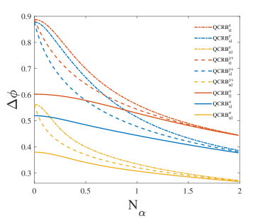
Figure 4: Phase sensitivity versus photon number $N_{\alpha}$ for different interferometer loss cases in the case of $\left|cat\right\rangle_{a}\otimes\left|\beta\right\rangle_{b}$ input with $\left|\beta\right|=0.5$, $g=1.2$, $\eta_{a}=0.5$ and $\eta_{b}=1$ (single-arms loss case), $\eta_{a}=\eta_{b}=0.5$ (two-arms loss case), and $\theta_{G}=\pi$. QCRB${}_{p}^{k}$: $k\in$[o, odd coherent states input case; e, even coherent states input case; ys, Yurke-Stoler states input case], $p\in$[nl, lossless case; sl, single-arm loss case; tl, two-arms loss case].

In the case of SU(1,1) interferometers, for phase sum estimation the optimal bound $\mathcal{C}_{\mathrm{cat}}^{\mathrm{opt}}$ for losses in one arm with arbitrary pure state input is worked out by Zeng et al. Zeng23 , which is given by:

$$\mathcal{C}_{\mathrm{cat}}^{\mathrm{opt}}=\frac{4}{\Upsilon}[\langle\hat{n}_{a}\rangle\frac{\eta_{a}}{1-\eta_{a}}\zeta^{2}\langle(\Delta n_{b})^{2}\rangle+\langle\hat{n}_{a}\rangle^{2}(\frac{\eta_{a}}{1-\eta_{a}})^{2}\kappa^{2}\zeta],\text{ \ }$$ (22)

where

$$\Upsilon=(\frac{\eta_{a}\langle\hat{n}_{a}\rangle}{1-\eta_{a}})^{2}\kappa^{2}(\langle(\Delta n_{a})^{2}\rangle+\langle(\Delta n_{b})^{2}\rangle-2Cov[\hat{n}_{a},\hat{n}_{b}])$$

$$+\langle\hat{n}_{a}\rangle\frac{\eta_{a}}{1-\eta_{a}}\zeta(2\kappa^{2}+\zeta)+\zeta^{2}\langle(\Delta n_{b})^{2}\rangle,$$ (23)

and

$$\zeta = \langle(\Delta n_{a})^{2}\rangle\langle(\Delta n_{b})^{2}\rangle-Cov[\hat{n}_{a},\hat{n}_{b}]^{2},$$

$$\kappa = \langle(\Delta n_{b})^{2}\rangle-Cov[\hat{n}_{a},\hat{n}_{b}].$$ (24)

The QFI for losses in two arms is given as follows:

$$\mathcal{C}_{\mathrm{cat}}=C_{ss}-\frac{C_{sd}C_{ds}}{C_{dd}},$$ (25)

where

$$C_{ss} = \overline{\left\langle\Delta\hat{n}_{a}^{2}\right\rangle}+\overline{\left\langle\Delta\hat{n}_{b}^{2}\right\rangle}+2\overline{Cov[\hat{n}_{a},\hat{n}_{b}]},$$

$$C_{dd} = \overline{\left\langle\Delta\hat{n}_{a}^{2}\right\rangle}+\overline{\left\langle\Delta\hat{n}_{b}^{2}\right\rangle}-2\overline{Cov[\hat{n}_{a},\hat{n}_{b}]},$$

$$C_{sd} = C_{ds}=\overline{\left\langle\Delta\hat{n}_{a}^{2}\right\rangle}+\overline{\left\langle\Delta\hat{n}_{b}^{2}\right\rangle},$$ (26)

where $\overline{\left\langle\Delta\hat{n}_{a}^{2}\right\rangle}=[1-\Gamma_{a}(1-\eta_{a})]^{2}\left\langle\Delta\hat{n}_{a}^{2}\right\rangle+\Gamma_{a}^{2}(1-\eta_{a})\eta_{a}\left\langle\hat{n}_{a}\right\rangle$, $\overline{\left\langle\Delta\hat{n}_{b}^{2}\right\rangle}=[1-\Gamma_{b}(1-\eta_{b})]^{2}\left\langle\Delta\hat{n}_{b}^{2}\right\rangle+\Gamma_{b}^{2}(1-\eta_{b})\eta_{b}\left\langle\hat{n}_{b}\right\rangle$, $\overline{Cov[\hat{n}_{a},\hat{n}_{b}]}=[1-\Gamma_{a}(1-\eta_{a})][1-\Gamma_{b}(1-\eta_{b})]Cov[\hat{n}_{a},\hat{n}_{b}]$, $\Gamma_{a}=\gamma_{a}+1$, and $\Gamma_{b}=\gamma_{b}+1$.

In the above expression (25), the matrix elements $C_{ij}$ are a function of $\Gamma_{a}$ and $\Gamma_{b}$. Then minimizing $\mathcal{C}_{\mathrm{cat}}$ by the parameters $\Gamma_{a}$ and $\Gamma_{b}$, the optimal $\Gamma_{a}^{\mathrm{opt}}$ and $\Gamma_{b}^{\mathrm{opt}}$ is obtained. Substituting $\Gamma_{a}^{\mathrm{opt}}$ and $\Gamma_{b}^{\mathrm{opt}}$ into $\mathcal{C}_{\mathrm{cat}}$, the minimum $\mathcal{C}_{\mathrm{cat}}^{\mathrm{opt}}$ is obtain, i.e., $\mathcal{F}_{\mathrm{cat}}$ in the presence of losses in two arms is achieved. However, $\mathcal{C}_{\mathrm{cat}}$ is more complex, and we cannot obtain an analytical solution, which can be shown by the numerical solution according to different input states.

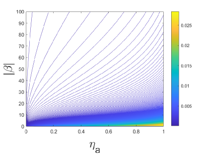
Figure 5: Phase sensitivity difference $\Delta\phi_{cat-sv}$ between $\left|cat\right\rangle_{a}\otimes\left|\beta\right\rangle_{b}$ and $\left|\xi\right\rangle_{a}\otimes\left|\beta\right\rangle_{b}$ input with $\bar{n}_{\alpha}=\bar{n}_{s}$ as a function of the photon loss factor $\eta_{a}$ and the amplitude $\left|\beta\right|$ of the coherent state. Parameters: $\alpha=2$, $g=1.2$, $\theta=\pi$ and $\theta_{G}=\pi$.

When the Schrödinger cat state and coherent state ($|cat\rangle_{a}\otimes|\beta\rangle_{b}$) input, the average number of photons and variances in the two arms, and the covariance are

$$\langle\hat{n}_{a}\rangle_{\mathrm{cat}} = \cosh^{2}(g)\bar{n}_{\alpha}+\sinh^{2}(g)(1+\left|\beta\right|^{2})+\bar{n}_{q},$$

$$\langle\hat{n}_{b}\rangle_{\mathrm{cat}} = \cosh^{2}(g)\left|\beta\right|^{2}+\sinh^{2}(g)(1+\bar{n}_{\alpha})+\bar{n}_{q},$$ (27)

and

$$\langle(\Delta n_{a})^{2}\rangle_{\mathrm{cat}} = \sinh^{4}(g)\left|\beta\right|^{2}+\sinh^{2}(g)\bar{n}_{q}$$

$$+\frac{1}{4}\sinh^{2}(2g)(2\bar{n}_{\alpha}\left|\beta\right|^{2}+\bar{n}_{\alpha}+\left|\beta\right|^{2}+1)$$

$$+\cosh^{2}(g)(1-2\alpha^{2}-2\bar{n}_{\alpha})\bar{n}_{q}$$

$$+\cosh^{4}(g)(\alpha^{4}+\bar{n}_{\alpha}-\bar{n}_{\alpha}^{2})+\bar{n}_{Q}-\bar{n}_{q}^{2},$$

$$\langle(\Delta n_{b})^{2}\rangle_{\mathrm{cat}} = \cosh^{4}(g)\left|\beta\right|^{2}+\cosh^{2}(g)\bar{n}_{q}$$

$$+\frac{1}{4}\sinh^{2}(2g)(2\bar{n}_{\alpha}\left|\beta\right|^{2}+\bar{n}_{\alpha}+\left|\beta\right|^{2}+1)$$

$$+\sinh^{2}(g)(1-2\alpha^{2}-2\bar{n}_{\alpha})\bar{n}_{q}$$

$$+\sinh^{4}(g)(\alpha^{4}+\bar{n}_{\alpha}-\bar{n}_{\alpha}^{2})+\bar{n}_{Q}-\bar{n}_{q}^{2},$$

$$cov(\hat{n}_{a},\hat{n}_{b})_{\mathrm{cat}} = \cosh(2g)(1-\bar{n}_{\alpha}-\alpha^{2})\bar{n}_{q}+\bar{n}_{Q}-\bar{n}_{q}^{2}$$ (28)

$$+\frac{1}{4}\sinh^{2}(2g)[\alpha^{4}+2\left|\beta\right|^{2}+1$$

$$+\bar{n}_{\alpha}(2+2\left|\beta\right|^{2}-\bar{n}_{\alpha})].$$

Similarly, for vacuum squeezed state and coherent state ($|\xi\rangle_{a}\otimes|\beta\rangle_{b}$) input we have

$$\langle\hat{n}_{a}\rangle_{\mathrm{sv}} = \cosh^{2}(g)\sinh^{2}r+\sinh^{2}(g)(\left|\beta\right|^{2}+1),$$

$$\langle\hat{n}_{b}\rangle_{\mathrm{sv}} = \cosh^{2}(g)\left|\beta\right|^{2}+\sinh^{2}(g)\cosh^{2}r,$$ (29)

$$\langle(\Delta^{2}n_{a})\rangle_{\mathrm{sv}} = \sinh^{4}(g)\left|\beta\right|^{2}+2\cosh^{4}(g)\sinh^{2}r\cosh^{2}r$$

$$+\frac{1}{4}\sinh^{2}(2g)(\left|\beta\right|^{2}e^{2r}+\cosh^{2}r),$$

$$\langle(\Delta n_{b})^{2}\rangle_{\mathrm{sv}} = \cosh^{4}(g)\left|\beta\right|^{2}+2\sinh^{4}(g)\sinh^{2}r\cosh^{2}r$$

$$+\frac{1}{4}\sinh^{2}(2g)(\left|\beta\right|^{2}e^{2r}+\cosh^{2}r),$$

$$cov(\hat{n}_{a},\hat{n}_{b})_{\mathrm{sv}} = \frac{1}{4}\sinh^{2}(2g)(\left|\beta\right|^{2}+\left|\beta\right|^{2}e^{2r}$$ (30)

$$+2\sinh^{2}r\cosh^{2}r+\cosh^{2}r).$$

The phase sensitivity versus photon number $N_{\alpha}$ with $|cat\rangle_{a}\otimes|\beta\rangle_{b}$ input is shown in Fig. 4. There are three cases: two arm loss case (light green lines), single arm loss case (blue lines) and lossless case (light yellow lines), and each case there are also three different cat states input: even coherent states (dashed-dotted lines), Yurke-Stoler states (dashed lines) and odd coherent states (solid lines). It is shown that the sensitivity of odd coherent state input is optimal with or without loss. The sensitivity decreases as the losses increase from one arm to two arms. As the coherent states of Schrödinger cat states increase, the quantum enhancement of phase sensitivity decreases and goes to $0$, where the Mandel $Q$-parameter $Q_{a_{in}}$ goes to $0$, and the effect of Schrödinger cat states is equivalent to coherent state.

Next, we numerically compare the loss resistance of the cat state and the squeezed vacuum state. Considering that there is loss in the arm of cat state and squeezed state, such as $\eta_{a}=50\%$, the phase sensitivity of them can still exceed SQL as shown in Fig. 3, where $\Delta\phi_{\mathrm{SQL}}=1/\sqrt{\langle\hat{N}\rangle}$ with $\langle\hat{N}\rangle$ the total number of photons. In the presence of loss, the sensitivity of squeezed state input is still better than cat state input, but the advantage of squeezed state input is smaller than lossless case. The phase sensitivity difference $\Delta\phi_{\mathrm{cat-sv}}$ as a function of $|\beta|$ and $\eta_{a}$ is shown in Fig. 5, where this difference between them becomes smaller and smaller as the loss (1-$\eta_{a}$) and amplitude of the input coherent state $|\beta|$ increase for given $\bar{n}_{\alpha}=$ $\bar{n}_{s}$. The numerical result $\Delta\phi_{\mathrm{cat-sv}}$ shows that the Schrödinger cat states are more resistant to loss than squeezed vacuum states.

V conclusion

In conclusion, we theoretically study the quantum enhancement of the parameter estimation by changing the quantum statistics of the Schrödinger cat state with it input the SU(1,1) interferometer. The phase sensitivity is dependent on the relative phase $\theta$ between two coherent states of Schrödinger cat states. The optimal sensitivity is achieved when the odd coherent states input with sub-Poissonian statistics. Compared with the squeezed vacuum state, the phase sensitivity of the odd coherent state is inferior, but is more resistant to loss. These results should be helpful in the practical application, such as quantum precision measurement, quantum sensing, and so on.

VI Acknowledgments

This work is supported by the Innovation Program for Quantum Science and Technology 2021ZD0303200; the National Natural Science Foundation of China Grants No. 11974111, No. 12274132, No. 12234014, No. 11654005, No. 11974116, No. 11874152, and No. 91536114; Shanghai Municipal Science and Technology Major Project under Grant No. 2019SHZDZX01; Innovation Program of Shanghai Municipal Education Commission No. 202101070008E00099; the National Key Research and Development Program of China under Grant No. 2016YFA0302001; Chinese National Youth Talent Support Program; and Fundamental Research Funds for the Central Universities. W. Z. acknowledges additional support from the Shanghai Talent Program.

References

• (1) B. Yurke, S. L. McCall, and J. R. Klauder, SU(2) and SU(1 1) interferometers, Phys. Rev. A 33, 4033 (1986).
• (2) C. W. Helstrom, Quantum Detection and Estimation Theory (Academic, New York, 1976).
• (3) A. S. Holevo, Probabilistic and Statistical Aspects of Quantum Theory (North-Holland, Amsterdam, 1982).
• (4) C. M. Caves, Quantum-mechanical noise in an interferometer, Phys. Rev. D 23, 1693(1981)
• (5) S. L. Braunstein and C. M. Caves, Statistical distance and the geometry of quantum states, Phys. Rev. Lett. 72, 3439 (1994).
• (6) S. L. Braunstein, C. M. Caves, and G. J. Milburn, Generalized uncertainty relations: Theory, examples, and Lorentz invariance, Ann. Phys. 247, 135 (1996).
• (7) H. Lee, P. Kok, and J. P. Dowling, J Mod, A quantum Rosetta stone for interferometry, Opt 49, 2325 (2002).
• (8) V. Giovannetti, S. Lloyd, and L. Maccone, Quantum Metrology, Phys. Rev. Lett. 96, 010401 (2006).
• (9) M. Zwierz, C. A. Pérez-Delgado, and P. Kok, General Optimality of the Heisenberg Limit for Quantum Metrology, Phys. Rev. Lett. 105, 180402 (2010).
• (10) V. Giovannetti, S. Lloyd, and L. Maccone, Quantum-Enhanced Measurements: Beating the Standard Quantum Limit, Science 306, 1330 (2004).
• (11) V. Giovannetti, S. Lloyd, and L. Maccone, Advances in quantum metrology, Nature photonics 5, 222 (2011).
• (12) F. Hudelist, J. Kong, C. Liu, J. Jing, Z. Y. Ou, and W. Zhang, Quantum metrology with parametric amplifier-based photon correlation interferometers, Nat. Commun. 5, 3049 (2014).
• (13) M. Xiao, L. A. Wu, and H. J. Kimble, Precision Measurement beyond the Short Noise Limit, Phys. Rev. Lett. 59, 278 (1987).
• (14) P. Grangier, R. E. Slusher, B. Yurke, and A. LaPorta, Squeezed-Light-Enhanced Polarization Interferometer, Phys. Rev. Lett. 59, 2153 (1987).
• (15) J. P. Dowling, Quantum optical metrology–the lowdown on high-N00N states, Contemporary Physics 49, 125 (2008).
• (16) A. N. Boto, P. Kok, D. S. Abrams,S. L. Braunstein, C. P. Williams, and J. P. Dowling, Quantum Interferometric Optical Lithography: Exploiting Entanglement to Beat the Diffraction Limit, Phys. Rev. Lett. 85, 2733 (2000).
• (17) C. C. Gerry and P. L. Knight, Introductory Quantum Optics (Cambridge University Press, Cambridge, 2005).
• (18) N. A. Ansari, L. Di Fiore, M. A. Man’ko, V. I. Man’ko, S. Solimeno, and F. Zaccaria, Quantum limits in interferometric gravitational-wave antennas in the presence of even and odd coherent states, Phys. Rev. A 49, 2151 (1994).
• (19) V. Buz̆ek, A. Vidiella-Barranco, and P. L. Knight, Superpositions of coherent states: Squeezing and dissipation, Phys. Rev. A 45, 6570 (1992).
• (20) N. A. Ansari and V. I. Man’ko, Photon statistics of multimode even and odd coherent light, Phys. Rev. A 50, 1942 (1994).
• (21) B. M. Escher, R. L. de Matos Filho and L. Davidovich, General framework for estimating the ultimate precision limit in noisy quantum-enhanced metrology, Nat. Phys. 7, 406 (2011).
• (22) R. Demkowicz-Dobrzanski, J. Kolodynski, and M. Guta, The elusive Heisenberg limit in quantum-enhanced metrology, Nat. Commun. 3, 1063 (2012).
• (23) R. Demkowicz-Dobrzanski, U. Dorner, B. J. Smith, J. S. Lundeen, W. Wasilewski, K. Banaszek, and I. A. Walmsley, Quantum phase estimation with lossy interferometers, Phys. Rev. A 80, 013825 (2009).
• (24) G. Toth and I. Apellaniz, Quantum metrology from a quantum information science perspective, J. Phys. A 47, 424006 (2014).
• (25) L. Pezzè and A. Smerzi, in Proceedings of the International School of Physics “Enrico Fermi”, Course CLXXXVIII “Atom Interferometry” edited by G. Tino and M. Kasevich (Società Italiana di Fisica and IOS Press, Bologna, 2014), p. 691.
• (26) R. Demkowicz-Dobrzanski, M. Jarzyna, J. Kolodynski, Quantum limits in optical interferometry, Progress in Optics 60, 345 (2015).
• (27) X.-B. Wang, T. Hiroshima, A. Tomita, M. Hayashi, Quantum information with Gaussian states, Opt. Reports 448, 1 (2007).
• (28) M. Jarzyna and R. Demkowicz-Dorbrzanski, Quantum interferometry with and without an external phase reference, Phys. Rev. A 85, 011801(R) (2012).
• (29) C. Sparaciari, S. Olivares, and M. G. A. Paris, Gaussian-state interferometry with passive and active elements, Phys. Rev. A 93, 023810 (2016).
• (30) A. Monras, Phase space formalism for quantum estimation of Gaussian states, arXiv:1303.3682v1 (2013).
• (31) O. Pinel, P. Jian, N. Treps, C. Fabre, and D. Braun, Quantum parameter estimation using general single-mode Gaussian states, Phys. Rev. A 88, 040102(R) (2013).
• (32) Jing Liu, Xiaoxing Jing, and Xiaoguang Wang, Phase-matching condition for enhancement of phase sensitivity in quantum metrology, Phys. Rev. A 88, 042316 (2013).
• (33) Y. Gao and H. Lee, Bounds on quantum multiple-parameter estimation with Gaussian state, Eur. Phys. J. D 68, 347 (2014).
• (34) Z. Jiang, Quantum Fisher information for states in exponential form, Phys. Rev. A 89, 032128 (2014).
• (35) D. Safranek, A. R. Lee, and I. Fuentes, Quantum parameter estimation using multi-mode Gaussian states, New J. Phys. 17, 073016 (2015).
• (36) C. Sparaciari, S. Olivares, and M. G. A. Paris, Bounds to precision for quantum interferometry with Gaussian states and operations, J. Opt. Soc. Am. B 32, 1354 (2015).
• (37) H. Strobel, W. Muessel, D. Linnemann, T. Zibold, D. B. Hume, L. Pezze, A. Smerzi, M. K. Oberthaler, Fisher information and entanglement of non-Gaussian spin states, Science 345, 424 (2014).
• (38) P. Hauke, M. Heyl, L. Tagliacozzo, and P. Zoller, Measuring multipartite entanglement through dynamic susceptibilities, Nat. Phys. 12, 778 (2016).
• (39) M. Takeoka, K. P. Seshadreesan, C. You, S. Izumi, and J. P. Dowling, Fundamental precision limit of a Mach-Zehnder interferometric sensor when one of the inputs is the vacuum, Phys. Rev. A 96, 052118 (2017).
• (40) W. Zhong, Y. Huang, X.Wang, and S.-L. Zhu, Optimal conventional measurements for quantum-enhanced interferometry, Phys. Rev. A 95, 052304 (2017).
• (41) J.-D. Zhang, Z.-J. Zhang, L.-Z. Cen, J.-Y. Hu, and Y. Zhao, Nonlinear phase estimation: Parity measurement approaches the quantum Cramér-Rao bound for coherent states, Phys. Rev. A 99, 022106 (2019).
• (42) M. D. Lang and C. M. Caves, Optimal Quantum-Enhanced Interferometry Using a Laser Power Source, Phys. Rev. Lett. 111, 173601 (2013).
• (43) M. D. Lang and C. M. Caves, Optimal quantum-enhanced interferometry, Phys. Rev. A 90, 025802 (2014).
• (44) S. Ataman, A. Preda, and R. Ionicioiu, Phase sensitivity of a Mach-Zehnder interferometer with single-intensity and difference-intensity detection, Phys. Rev. A 98, 043856 (2018).
• (45) C. You, S. Adhikari, X. Ma, M. Sasaki, M. Takeoka, and J. P. Dowling, Conclusive precision bounds for SU(1,1) interferometers, Phys. Rev. A 99, 042122 (2019).
• (46) W. Zhong, F. Wang, L. Zhou, P. Xu, and Y. Sheng, Quantum-enhanced interferometry with asymmetric beam splitters, Sci. China Phys. Mech. Astron. 63, 260312 (2020).
• (47) J. Jing, C. Liu, Z. Zhou, Z. Y. Ou, and W. Zhang, Realization of a nonlinear interferometer with parametric amplifiers, Appl. Phys. Lett. 99, 011110 (2011).
• (48) B. Chen, C. Qiu, S. Chen, J. Guo, L. Q. Chen, Z. Y. Ou, and W. Zhang, Atom-Light Hybrid Interferometer, Phys. Rev. Lett. 115, 043602 (2015).
• (49) P. Kok and B.W. Lovett, Introduction to Optical Quantum Information Processing, Cambridge University Press, 2010.
• (50) Q.-K. Gong, X.-L. Hu, D. Li, C.-H. Yuan, Z. Y. Ou, and W. Zhang, Intramode correlations enhanced phase sensitivities in an SU(1,1) interferometer, Physical Review A 96, 033809 (2017).
• (51) J. Zeng, D. Li, L. Q. Chen, W. Zhang, and C.-H. Yuan, Ultimate precision limit of SU(2) and SU(1,1) interferometers in noisy metrology, arXiv:2302.09823