Combining observational and experimental data for causal inference considering data privacy

Abstract

Combining observational and experimental data for causal inference can improve treatment effect estimation. However, many observational data sets cannot be released due to data privacy considerations, so one researcher may not have access to both experimental and observational data. Nonetheless, a small amount of risk of disclosing sensitive information might be tolerable to organizations that house confidential data. In these cases, organizations can employ data privacy techniques, which decrease disclosure risk, potentially at the expense of data utility. In this paper, we explore disclosure limiting transformations of observational data, which can be combined with experimental data to estimate the sample and population average treatment effects. We consider leveraging observational data to improve generalizability of treatment effect estimates when a randomized experiment (RCT) is not representative of the population of interest, and to increase precision of treatment effect estimates. Through simulation studies, we illustrate the trade-off between privacy and utility when employing different disclosure limiting transformations. We find that leveraging transformed observational data in treatment effect estimation can still improve estimation over only using data from an RCT.

1 Introduction

A growing literature is developing ways to combine experimental and observational studies for causal inferences (Colnet et al., 2021). While treatment effect estimates from randomized experiments (RCTs) can be free from confounding bias, observational studies generally provide a richer source of information on a population of interest. The internet has given rise to more observational datasets that may be used to address the same questions as randomized experiments. Therefore, there should be more opportunities to leverage observational and RCT data together for improved treatment effect estimation. However, in practice it is not always the case that a researcher has access to both sources of data due to data privacy Snoke and Bowen (2020).

Many government agencies have useful data that they cannot release to the public in order to preserve data privacy. Data privacy refers to the right of individuals whom the data describe to control what information about themselves is shared Fellegi (1972); Raghunathan (2021). Typically sensitive data that is released to the public is sanitized in various ways, which potentially render the released data less useful. For example, only aggregate statistics or a sample of the data may be released, or small values are censored. There is a trade-off to consider, between data privacy, a right to be upheld, and the amount of information researchers can access to answer societal questions.

Balancing data privacy and releasing useful information is ultimately a policy decision. There are currently no overarching policies in the U.S. regulating data privacy or confidentiality Schwartz (2013); Bellovin et al. (2018). Rather, data privacy is legislated on a sector-by-sector basis Schwartz (2013). For example, patient, student, financial, and additional data from U.S. governmental agencies data are protected by separate acts: HIPPA, FERPA, FCRA, and CIPSEA (Health Insurance Portability and Accountability Act; Family Educational Rights and Privacy Act; Fair Credit Reporting Act; Confidential Information Protection and Statistical Efficiency Act) Schwartz (2013); Wood et al. (2018). On the other hand, members of the European Union and other countries throughout the world have adopted data privacy legislation with broad scopes across sectors Schwartz (2013). We do not address the legality of different approaches to data privacy. Rather, we raise these issues to establish that data stewards operate in different legal contexts, which may or may not provide specific procedures for protecting data privacy. In this paper we illustrate the trade-off between privacy and utility when combining experimental and observational data for causal inference. This could inform data stewards who want to release data that is as useful as possible while balancing data privacy.

We consider the setting in which analysts of an RCT could use auxiliary, observational data to improve treatment effect estimation, but the relevant auxiliary data cannot be released. In this paper, we explore ways that stewards of observational data could transform the data to preserve data privacy, so that it could be combined with experimental data for treatment effect estimation. While there are many ways to combine observational and experimental data that can improve estimation, we consider leveraging auxiliary data to (1) estimate treatment effects for a population of interest when the RCT sample is not representative of that population and (2) increase precision of RCT estimates. Through simulation studies, we explore the utility of different disclosure limiting transformations of auxiliary data for such estimation. We aim to encourage conversation between the literature that combines experimental and observational data for causal inference and the data privacy literature.

This paper is organized as follows. Section 2 establishes notation and the causal estimands and estimators of interest. Section 3 provides background on data privacy techniques and presents disclosure limiting transformations of auxiliary data. Section 4 describes simulation studies to evaluate the utility of the proposed transformations in treatment effect estimation that integrates transformed auxiliary data and RCT data and discusses the results. Section 5 concludes.

2 Leveraging Observational and Experimental Data in Causal Inference

The presentation in this section primarily follows Colnet et al. (2021). Consider a randomized experiment with $n$ subjects and a related auxiliary, observational, study with $m$ subjects, sampled from some population. For example, in a medical trial conducted to evaluate a treatment for sleep apnea there may also be electronic health records for thousands of patients across a country with sleep apnea. We denote $\mathcal{R}=\{i:1,...,n\}$ as the index set for subjects in the randomized experiment and $\mathcal{O}=\{i:n+1,...,m+n\}$ as the index set for subjects in the auxiliary (observational) study. Let $S_{i}$ be an indicator of whether subject $i$ is in the RCT sample, and $\pi_{i}^{S}=P(S_{i}=1)$ be the probability of selection into the RCT. The probability of selection into the RCT may depend on subject $i$’s observable characteristics, so that the RCT sample is not necessarily representative of the population. Let $T$ be a binary treatment indicator so $T_{i}=1$ if subject $i$ is assigned to treatment and $T_{i}=0$ if subject $i$ is assigned to control. We assume the probability that a subject in the RCT is assigned treatment, $\pi_{i}=P(T_{i}=1),0<\pi_{i}<1$, is known. In the setting we consider, we do not require the treatment to be observed in the observational study. Throughout this paper, the following conventions will be used: fixed quantities are in lowercase, random quantities are in uppercase, scalars are non-bolded, and vectors or matrices are bolded.

Following Neyman et al. (1935) and Rubin (1974), each subject has two potential outcomes, one which would be observed if treated, $Y^{t}_{i}$, and the other under control, $Y^{c}_{i}$. The observed outcome is a function of the potential outcomes and the treatment assignment: $Y_{i}=T_{i}Y^{t}_{i}+(1-T_{i})Y^{c}_{i}.$

Researchers may be interested in a number of causal estimands. This work explores integrating experimental and observational data, under data privacy considerations, to estimate the the population average treatment effect (PATE), as well as the RCT sample average treatment effect (SATE). The PATE is the expected treatment effect for a population of interest: $\tau_{PATE}=\mathbb{E}[Y^{t}-Y^{c}]$. The SATE is the expected treatment effect for an RCT sample: $\tau_{SATE}=\mathbb{E}[Y^{t}-Y^{c}|S=1]$. Combining experimental and observational data can improve estimating both the PATE and the SATE in different ways, as discussed in the following sections.

2.1 Generalizing to Populations of Interest

Treatment effects estimated only with an RCT do not necessarily generalize to a population of interest. Consider estimating the PATE for the population from which subjects of an RCT were sampled. If the subjects in the RCT are systematically different from this population (i.e., there is some selection bias to inclusion in the RCT), and the treatment effect depends on subject characteristics, then an estimate of the PATE with only the RCT data is biased. Further it will be unclear how “far off” the estimate is. In this case, we say that the RCT estimate does not generalize to the population. Observational studies are often more representative of the population from which they were sampled. Therefore, to estimate the PATE, it is useful to leverage information from an auxiliary observational study.

The literature proposes a number of estimates for the PATE which integrate experimental and observational data (Cole and Stuart, 2010; Stuart et al., 2011; Lesko et al., 2017; Dahabreh et al., 2019; Lee et al., 2021). See Colnet et al. (2021) for a full review. We consider the calibration weighted (CW) estimator proposed by Lee et al. (2021) because a statistical summary of auxiliary data is sufficient for this approach.

The CW estimator Lee et al. (2021) is a variation of the inverse probability weighted (IPW) estimator (Horvitz and Thompson, 1952; Robins et al., 1994),

$$\hat{\tau}^{IPW}=\sum_{i\in\mathcal{R}}\Big{[}T_{i}\frac{Y_{i}}{\pi_{i}}-(1-T_{i})\frac{Y_{i}}{1-\pi_{i}}\Big{]}.$$

The IPW estimator only uses data from the RCT ($i\in\mathcal{R})$ so it may be biased for the PATE. The CW estimator re-weights the RCT subjects in the IPW estimator. After weighting, the empirical covariate distribution of the RCT subjects more closely matches that of the auxiliary subjects ($i\in\mathcal{O})$ (which are assumed to represent the population of interest). Let ${\bm{X}_{i}}$ denote the vector of observed covariates for subject $i$. The CW estimator is defined as:

$$\hat{\tau}^{CW}=\sum_{i\in\mathcal{R}}\hat{w}({\bm{X}_{i}})\Big{[}T_{i}\frac{Y_{i}}{\pi_{i}}-(1-T_{i})\frac{Y_{i}}{1-\pi_{i}}\Big{]}$$

Each subject $i\in\mathcal{R}$ is assigned a weight $\hat{w}(\cdot)$, which is estimated using covariates from the auxiliary study and the RCT, solving the optimization problem: $\underset{w_{1},...,w_{n}}{\min}\sum_{i=1}^{n}w_{i}\log w_{i}$, subject to $w_{i}\geq 0$, $\sum_{i=1}^{n}w_{i}=1$ and

$$\sum_{i\in\mathcal{R}}w_{i}g({\bm{X}_{i}})=\frac{1}{m}\sum_{i\in\mathcal{O}}g({\bm{X}_{i}}).$$ (1)

Equation 1 is the key restriction on $w_{i}$ for generalizability - the goal is for the weighted sum of $g({\bm{X}_{i}})$ in the RCT sample to be equal to the simple mean of $g({\bm{X}_{i}})$ in the auxiliary sample. Two reasonable choices for $g(\cdot)$ would be $g(\bm{z})=\bm{z}$ and $g(\bm{z})=\bm{z}\bm{z}^{\prime}$. With these choices, the first or second empirical moments of the RCT sample covariates are calibrated to those moments of the auxiliary sample covariates since $\frac{1}{m}\sum_{i\in\mathcal{O}}g({\bm{X}_{i}})$ is a consistent estimator of $E[g(\bm{X})]$ for the auxiliary study. Lee et al. (2021) note that the calibration weighting estimator is a consistent estimator for the PATE if either (1) the probability of RCT participation can be modeled as $\exp\{\eta_{0}^{T}g(\bm{X})\}$ for some $\eta_{0}$ or (2) the conditional average treatment effect is a linear function of $g(\bm{X})$.

2.2 Improving Experimental Precision

We next consider a context in which the treatment effect for only an RCT sample is of interest. Even though there may no longer be a larger population of interest, incorporating information from observational data can still prove useful, in this case by improving the precision of an estimate of the SATE.

RCTs often have small sample sizes, so RCT estimates of the SATE may lack precision. A common approach to improving precision is covariate adjustment. Covariate adjustment accounts for variance in $Y_{i}$ which is not due to the treatment, but rather some observed covariates. A popular adjusted estimator for the SATE is the estimated coefficient for the treatment assignment in a regression model. One might consider a linear model $Y_{i}=\alpha+\tau T_{i}+\bm{\beta}{\bm{X}_{i}}+\varepsilon_{i}$ with the standard OLS assumptions. We denote the regression estimator for the SATE, estimated using OLS and the RCT covariates, as ${\hat{\tau}^{OLS}({\bm{X}}_{\{i\in\mathcal{R}\}})}$. The increase in precision achieved by covariate adjustment depends on how much of the variance in $Y_{i}$ can be explained by the observed covariates.

Because observational studies typically have much larger sample sizes than randomized experiments ($m>>n$), including information from an auxiliary study can improve precision more than covariate adjustment with the RCT sample alone. There are various ways that auxiliary information can be integrated into RCT analysis to improve precision (Pocock, 1976; Viele et al., 2014; Aronow and Middleton, 2013; Deng et al., 2013; Gui, 2020; Opper, 2021; Gagnon-Bartsch et al., 2021). For example, one part of the literature leverages historical controls from observational studies or previously run RCTs to improve precision in RCT estimates by pooling the different sources of data (Pocock, 1976; Viele et al., 2014). We focus on an approach that uses auxiliary observational data to construct a highly predictive covariate for the outcome of interest in the RCT.

Let $\hat{Y}_{i}$ denote a prediction for subject $i$ from a model fit on the auxiliary data and ${\hat{\bm{Y}}_{\mathcal{O}}}$ denote the $n\times 1$ vector of such predictions for the RCT subjects ($i\in\mathcal{R}$). Especially when there are a large number of covariates, a model fit on (large) auxiliary data will potentially be more informative of the outcome of interest than a model fit on (small) RCT data. For this reason, we expect ${\hat{\bm{Y}}_{\mathcal{O}}}$ to be a powerful covariate to adjust for the variability in the RCT outcome, which is not explained by the treatment assignment. We replace the RCT covariates with ${\hat{\bm{Y}}_{\mathcal{O}}}$ in the regression estimator, which can improve precision beyond covariate adjustment with the RCT covariates Opper (2021); Gagnon-Bartsch et al. (2021). We denote this regression estimator, using the auxiliary prediction as a covariate as ${\hat{\tau}^{OLS}({\hat{\bm{Y}}_{\mathcal{O}}})}$. We focus on this estimator for the SATE, integrating experimental and observational data, because all that is required from the auxiliary data is a model of the outcome of interest.

3 Disclosure Limiting Transformations of Auxiliary Data

In the previous section we discussed two estimators that combine experimental and observational data. In practice, one entity may not have access to both types of data. We assume that analysts with access to a randomized experiment are interested in incorporating information from a relevant auxiliary, observational, study. However, the data stewards of the auxiliary study cannot release the data ($(Y_{i},{\bm{X}_{i}}),i\in\mathcal{O}$) due to data privacy. Therefore, we consider transformations of the restricted auxiliary data that limit disclosure risk and can be used in the estimators discussed in the previous section (${\hat{\tau}^{CW}}$ and ${\hat{\tau}^{OLS}({\hat{\bm{Y}}_{\mathcal{O}}})}$). In this section we introduce data privacy frameworks (3.1), define the disclosure limiting transformations that we compare in this work (3.2 and 3.3), and discuss the trade-off between privacy and utility (3.4).

3.1 Data Privacy

With the rise of the internet and an explosion of data availability, computer scientists and statisticians have been considering issues of data privacy for the past four decades (see Duncan and Pearson, 1991; Fienberg, 2000; Aggarwal and Yu, 2008; Matthews and Harel, 2011; Salas and Domingo-Ferrer, 2018; Slavkovic and Seeman, 2022, for reviews). Two distinct but related concepts are data privacy and data confidentiality. Data privacy is defined as the right of individuals to control information about themselves Fellegi (1972). Data confidentiality is the agreement between individuals and data stewards regarding the extent to which others can access any private/sensitive information provided Fellegi (1972); Raghunathan (2021). Disclosure risk refers to the risk that an attacker could access sensitive information from released data. Historically there was a focus on microdata, data which has information at an individual level and includes information that could be used to identify an individual, however more recent work considers the risk of disclosure for statistical summaries (Slavkovic and Seeman, 2022). The goal of data privacy methods is to reduce disclosure risk.

We can view data privacy techniques as falling into two primary frameworks: statistical disclosure control (SDC) and differential privacy (DP) (see Slavkovic and Seeman, 2022; Raghunathan, 2021, for detailed discussions). SDC aims to uphold data privacy by maintaining data confidentiality. SDC techniques include, for example, synthetic data, cell suppression, data swapping, matrix masking and noise additions to limit the risk for disclosure of individual identities and attributes Matthews and Harel (2011). There is not one measure of disclosure risk in the SDC framework. On the other hand, the DP framework provides a mathematical definition for disclosure risk, although for a specific type of risk (discussed in the following section). We consider techniques under both frameworks in this paper, and use the term disclosure limitation to mean limiting the risk of disclosing sensitive information, not specifically referring to SDC.

3.1.1 Differential Privacy

Dwork et al. (2006); Dwork (2006) introduced differential privacy in the early 2000’s. Differential privacy is considered the first rigorous mathematical quantification of disclosure risk for privacy-preserving algorithms. Differentially private algorithms limit the difference in distribution between outputs of the algorithm generated from datasets that differ by only one observation Bowen and Garfinkel (2021).

Consider a private dataset $\bm{d}$ and a dataset $\bm{d}^{\prime}$ which is a subset of $\bm{d}$, differing by one observation. Formally, a random algorithm $\mathcal{K}$ achieves $\epsilon$-differential privacy if

$$\frac{P(\mathcal{K}(\bm{d})\in R)}{P(\mathcal{K}(\bm{d}^{\prime})\in R)}\leq\exp(\epsilon)$$

for all ($\bm{d},\bm{d}^{\prime}$) and all $R\subseteq\mbox{image}(\mathcal{K})$. This is the typical representation of the bound, which is agnostic to whether $\bm{d}$ or $\bm{d}^{\prime}$ is in the denominator. The parameter $\epsilon>0$ is chosen by the researcher and can be thought of as a “privacy budget.” The smaller the privacy budget $\epsilon$, the less risk of disclosure.

Algorithms that achieve $\epsilon$-differential privacy can be impractical as the outputs may not resemble the restricted statistics closely enough to be useful. Therefore, multiple relaxations have been developed including $(\epsilon,\delta)$-differential privacy (Dwork and Smith, 2010) which guarantees that:

$$P(\mathcal{K}(\bm{d})\in R)\leq P(\mathcal{K}(\bm{d}^{\prime})\in R)\exp(\epsilon)+\delta$$

In other words, $\mathcal{K}$ achieves $\epsilon$-differential privacy with probability $1-\delta$. We will focus on $(\epsilon,\delta)$-differential privacy in this paper. A common algorithm which achieves $(\epsilon,\delta)$-differential privacy is the Gaussian mechanism (Dwork and Roth, 2013), which adds random Gaussian noise to a statistic (called a query in the literature) calculated from the restricted data. Let $f(\bm{d})\in\mathbb{R}^{k},k\geq 1$ be a statistic, then $\mathcal{K}(\bm{d},\gamma)=f(\bm{d})+N_{k}(0,\gamma\bm{I})$. $\mathcal{K}(\bm{d},\gamma)$ achieves $(\epsilon,\delta)$-differential privacy when

$$\gamma=\Delta f\sqrt{2\log(1.25/\delta)}/\epsilon$$

$$\Delta f=\max\limits_{\bm{d},\bm{d}^{\prime}}||f(\bm{d}^{\prime})-f(\bm{d})||_{2}.$$

The researcher chooses $\epsilon$ and $\delta$, and $\Delta f$ is a straightforward calculation from the confidential data.

Differentially private algorithms maintain a couple of benefits. First, the definition makes no assumptions about the information that an attacker has. Differentially private algorithms are also robust to post processing, so any transformation of a differentially private output is still differentially private. When multiple statistics are calculated from the same data, the amount of privacy budget used for each statistic is simply added to calculate the total privacy budget used, called composition. The composition of a $(\epsilon_{1},\delta_{1})$-differentially private algorithm and a $(\epsilon_{2},\delta_{2})$-differentially private algorithm applied to the same data is a $(\epsilon_{1}+\epsilon_{2},\delta_{1}+\delta_{2})$-differentially private algorithm. Therefore, to maintain $(\epsilon,\delta)$-differential privacy among $q$ different statistics $f(\bm{d})$ from the same data, a $(\epsilon/q,\delta/q)$-differentially private algorithm is applied to each statistic.

There is a clear trade-off between the privacy budget $(\epsilon,\delta)$ and the magnitude of the noise added to the statistic ($\gamma$). The magnitude of the noise added to statistics additionally depends on the sensitivity of statistics to changing one observation in the confidential data (therefore, the largest outlier) and increases with the number of statistics calculated from the data. Therefore, the magnitude of the noise added can be so large that the transformed data is no longer useful, if the privacy budget is small.

Organizations have started adopting differential privacy for disclosure limitation in recent years Wood et al. (2018). Notably, the U.S. Census Bureau implemented a differentially private algorithm for releases of the 2020 Census redistricting data with $\epsilon=17.14,\delta=10^{-10}$ (Jarmin, 2021). There are no guidelines for choosing the privacy budget $\epsilon$ and $\delta$, which is ultimately a policy choice Bowen and Garfinkel (2021). In general, organizations currently use large privacy budgets because they make many queries from the same dataset. For example, in 2020 Google had a monthly privacy budget of $\epsilon\approx 80$ for Mobility Reports Rogers et al. (2020).

3.2 Synthetic Data

Rubin (1993) introduced the idea of generating and releasing a synthetic version of the data when raw microdata cannot be released. Rubin (1993) and Little (1993) viewed synthetic data as a missing data problem, where the sensitive information was missing and could be imputed with multiple imputation. In general, synthetic data replaces sensitive information in the original data with values generated from statistical summaries of the original data Snoke et al. (2018); Raghunathan (2021). We focus on fully synthetic data in this paper, where all of the observations and attributes are synthesized. Even though no observations from the confidential data are released in such synthetic data, there is still a risk of information disclosure Bellovin et al. (2018). A popular parametric method for data synthesis generates variable sequentially, generating the next variable with a model fit on the already synthesized variables (Nowok et al., 2016). Recently, methods have been developed to generate differentially private synthetic data Wilchek and Wang (2021); Boedihardjo et al. (2022). Synthetic data is appealing as a disclosure limiting transformation of confidential data because it can technically be analyzed with the same methods as the original data. Making valid inferences with synthetic data requires clear communication from the data steward to the public of how the data can be analyzed.

3.3 Noise Additions to the Gram Matrix

The major benefit of synthetic data is that it is at the same observation level as the confidential data that cannot be released. However, the estimators discussed in Section 2 do not require the individual level auxiliary data. Estimating the PATE with ${\hat{\tau}^{CW}}(\cdot)$, only requires the first or second empirical moments of the auxiliary data. Estimating the SATE with ${\hat{\tau}^{OLS}({\hat{\bm{Y}}_{\mathcal{O}}})}$, only requires predictions from a model fit of the covariates on the outcome of interest with the auxiliary data. Therefore, we consider statistical summaries of the auxiliary data to limit disclosure risk.

We define the data matrix $\bm{D}_{m\times p+2}$ with observations $\bm{D}_{i}=(1,Y_{i},{\bm{X}_{i}})$. Let $\bm{Y}$ denote the $m\times 1$ vector of observed outcomes, ${\bm{X}}$ denote the $m\times p$ matrix of covariates, and $\bm{1}$ denote a $m\times 1$ vector of 1’s. Then, the gram matrix of the data matrix ${\bm{G}}=\bm{D}^{\prime}\bm{D}/m$ includes ${\bm{X}}^{\prime}{\bm{X}}/m$, ${\bm{X}}^{\prime}\bm{Y}/m$, $\hat{\mu}_{Y}=\bm{1}^{\prime}\bm{Y}/m$, and $\hat{\bm{\mu}}_{x}=\bm{1}^{\prime}{\bm{X}}/m$. The coefficients $\bm{\beta}$ for an OLS model are estimated as $\hat{\bm{\beta}}=({\bm{X}}^{\prime}{\bm{X}})^{-1}{\bm{X}}^{\prime}\bm{Y}$, so ${\bm{G}}$ is sufficient to estimate $\hat{\bm{\beta}}$ for the auxiliary study to leverage in ${\hat{\tau}^{OLS}({\hat{\bm{Y}}_{\mathcal{O}}})}$. ${\bm{G}}$ includes the first and second empirical moments of $\bm{D}$, to leverage in ${\hat{\tau}^{CW}}(\cdot)$.

Therefore, the gram matrix of the auxiliary data ${\bm{G}}$ seems like a sensible place to start for a disclosure limiting transformation of the data. In fact, ${\bm{G}}=\bm{D}^{\prime}\bm{D}/m$ is a special version of matrix masking, a SDC technique Duncan and Pearson (1991). However, this type of matrix masking does not meet current standards for disclosure limitation, so we propose releasing a noisy version of the gram matrix of the auxiliary data. We explore two approaches to adding noise, discussed in the following sections.

3.3.1 Differentially Private (DP) Transformation

${\bm{G}}$ is a symmetric matrix of statistics calculated from the data $\bm{D}$. Therefore, we can think of the upper triangle of ${\bm{G}}$ as a vector of statistics with length $k=\frac{1}{2}(p^{2}+5p+2)$ and could apply the Gaussian mechanism as described in Section 3.1.1 to this vector with some privacy budget $(\epsilon,\delta)$. However, the magnitude of the Gaussian noise added to each element of the vector depends on the largest difference of the upper triangle of ${\bm{G}}$ given one observation is removed. The columns of $\bm{D}$ might be on vastly different scales and with different variances. This is therefore not the best approach to attain $(\epsilon,\delta)$-differential privacy while adding as little noise as possible.

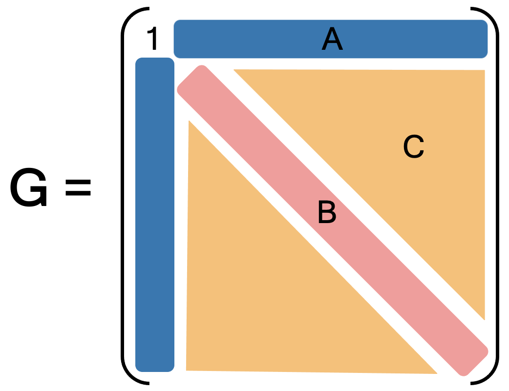
Figure 1: Illustration of how the gram matrix ${\bm{G}}$ can be partitioned into separate parts, which correspond to the column means (A), empirical second moments (B) and empirical moments of the columns cross multiplied (C).

Instead, we divide the upper triangle of ${\bm{G}}$, including the diagonal, into different elements, as illustrated in Figure 1, and divide the privacy budget among those elements. Define the vector of column means, $\hat{\bm{\mu}}=(\hat{\mu}_{Y},\hat{\bm{\mu}}_{x})$, the vector of column variances $\hat{\bm{\sigma}}^{2}=((\bm{Y}-{\bm{1}}\hat{\mu}_{Y})^{\prime}(\bm{Y}-{\bm{1}}\hat{\mu}_{Y})/m,\mathrm{diag}[({\bm{X}}-{\bm{1}}\hat{\bm{\mu}}_{x})^{\prime}({\bm{X}}-{\bm{1}}\hat{\bm{\mu}}_{x})/m])$, and the correlation matrix $\hat{\bm{R}}_{p+1\times p+1}$ of $\bm{D}$. Then, $\bm{G}$ can be reconstructed as illustrated in Figure 1 with A = $\hat{\bm{\mu}}$, B = $\hat{\bm{\sigma}}^{2}+\hat{\bm{\mu}}^{2}$ (where the square on $\hat{\bm{\mu}}^{2}$ is defined entrywise), and C is the upper triangle of a matrix $\hat{\bm{C}}$ with $\hat{\bm{C}}_{\ell,j}$ = $\hat{\bm{R}}_{\ell,j}\hat{\bm{\sigma}}_{\ell}\hat{\bm{\sigma}}_{j}+\hat{\bm{\mu}}_{\ell}\hat{\bm{\mu}}_{j}$. We construct $(\epsilon,\delta)-$differentially private ${\bm{G}}$ as follows:

1. Calculate $\hat{\bm{\mu}}$, $\hat{\bm{\sigma}}$, and $\hat{\bm{R}}$.

2. Apply the Gaussian mechanism to each element of $\hat{\bm{\mu}}$ and $\hat{\bm{\sigma}}$ with a portion of the privacy budget, generating $\hat{\bm{\mu}}_{dp},\hat{\bm{\sigma}}_{dp}$.

3. Treat the upper triangle, non-diagonal entries of $\hat{\bm{R}}$ as a vector and apply the Gaussian mechanism with the remainder of the privacy budget to generate $\hat{\bm{R}}_{dp}$.

4. Reconstruct a differentially private gram matrix ${\bm{G}^{\ast}}$ using $\hat{\bm{\mu}}_{dp}$ and $\hat{\bm{\sigma}}_{dp}$, and $\hat{\bm{R}}_{dp}$.

We divide the privacy budget between $\hat{\bm{\mu}}$, $\hat{\bm{\sigma}}$, and the upper triangle of $\hat{\bm{R}}$ proportionally to the number of elements in each. Therefore, $\hat{\bm{\mu}}$ and $\hat{\bm{\sigma}}$ are allocated $\frac{2(p+1)}{p^{2}+5p+4}$ and the upper triangle of $\hat{\bm{R}}$ is allocated $\frac{p^{2}+p}{p^{2}+5p+4}$ of the privacy budget. We apply the Gaussian mechanism to each element of $\hat{\bm{\mu}}$ and $\hat{\bm{\sigma}}$ separately, so the privacy budget is further divided by $p+1$ for each element. Due to the composition theorem, the resulting noisy gram matrix ${\bm{G}^{\ast}}$ is $(\epsilon,\delta)-$differentially private. Dividing the gram matrix into these elements allows adding a smaller magnitude of noise while still achieving differential privacy – $\hat{\bm{R}}$ is calculated after first scaling columns of $\bm{D}$ and applying the Gaussian mechanism element-wise to $\hat{\bm{\mu}}$ and $\hat{\bm{\sigma}}$ accounts for scale differences between columns.

3.3.2 Entry-wise Noise (EN) Transformation

When adding noise after computing ${\bm{G}}$, as in the DP transformation, there is no guarantee that the properties of a gram matrix (e.g. positive definiteness) will be maintained. Therefore, as an alternative approach, we propose adding a small amount of random noise to each entry of the auxiliary data, and then calculating the gram matrix from this noisy version of the data. Formally, let $\bm{E}$ be a matrix of random noise, then calculate $\bm{\tilde{}}{\bm{D}}=\bm{D}+\bm{E}$ and release ${\tilde{\bm{G}}}=\tilde{\bm{D}}^{\prime}\tilde{\bm{D}}$. Therefore, ${\tilde{\bm{G}}}$ is a legitimate gram matrix, and maintains the associated properties. An additional benefit is that fitting OLS with ${\tilde{\bm{G}}}$ has a nice interpretation as an error in variables model. A reasonable choice for the variance of the noise added to each element is the variance of the element’s column, which can be estimated with the empirical variance.

We do not provide a quantification of the disclosure limitation achieved by this entry-wise noise (EN) transformation in this paper. In practice, data stewards may use different measures of disclosure risk (see, for example Slavkovic and Seeman, 2022, §2.2). Within the SDC framework, data stewards might choose the magnitude of noise to add to each element of $\bm{D}$, evaluate the risk of disclosure based on that choice, then increase or decrease the noise based on that evaluation and repeat until disclosure risk is suitably low Bowen (2021).

3.4 Privacy-Utility Trade-off

With any disclosure limiting procedure, there is a trade-off between privacy and utility Matthews and Harel (2011); Bowen (2021); Slavkovic and Seeman (2022). To maximize utility, analysts would want the original data, and thus there would be no data privacy. On the other hand, for there to be no disclosure risk, the data could not be released, so there would be no utility. Data stewards therefore must decide on a tolerable disclosure risk and a measure of data utility in order to balance the two competing forces. This is not a trivial task. As discussed in Section 1, depending on the context, there are not necessarily formal guidelines for determining a tolerable disclosure risk. Additionally, anticipating all of the desired uses of a dataset is not feasible.

In this paper, we consider specific measures of utility: the mean squared error (MSE) of ${\hat{\tau}^{CW}}(\cdot)$ and variance of ${\hat{\tau}^{OLS}({\hat{\bm{Y}}_{\mathcal{O}}})}$. We do not specify a tolerable disclosure risk. Rather, the simulation studies in the following section explore the privacy-utility trade-off when employing the disclosure limiting transformations discussed above.

4 Simulation Studies

We conduct two simulation studies to compare the utility of privacy transformed auxiliary data in estimators of the PATE and SATE respectively. As baselines, we use the simple difference (or difference-in-means) estimator $\hat{\tau}^{DM}$ and regression estimator ${\hat{\tau}^{OLS}({\bm{X}}_{\{i\in\mathcal{R}\}})}$, which only rely on RCT data. The simple difference estimator is the difference in the mean outcomes for the subjects assigned treatment and those assigned control. These are compared to the calibration weighted estimator and regression estimator incorporating the disclosure limiting transformations of the auxiliary data, discussed in Sections 3.2 and 3.3.

4.1 Generalizing to Populations of Interest

We consider a setting where there is an RCT and a related observational study which were both sampled from a population of interest. The aim is to estimate the PATE for this population of interest. The auxiliary study is representative of this population. However, the RCT sample is not representative of the population of interest due to selection bias. We consider a modified version of the simulations in Colnet et al. (2021) and Lee et al. (2021), which assumes a heterogeneous treatment effect.

For $p=10$ and $p=20$, we repeat the following procedure 1,000 times. We emulate a hypothetical randomized experiment and auxiliary study assuming that the SATE in the RCT does not equal the desired PATE due to selection bias. We generate the $1\times p$ covariate vector ${\bm{X}_{i}}$ from i.i.d $N(\bm{1},\bm{I}_{p})$ distributions. We additionally generate a covariate $X^{S}_{i}\sim N(1,1)$, which impacts both selection into the RCT and subject $i$’s treatment effect. Let $S_{i}$ be an indicator of whether subject $i$ is selected into the RCT and $\pi_{i}^{S}=P(S_{i}=1)$. We model the probability of selection into the RCT with a logistic regression model:

$$\mbox{logit}\{\pi_{i}^{S}\}=-2+\bm{\beta}_{S}{\bm{X}_{i}}+.5X^{S}_{i}.$$

$\bm{\beta}_{S}$ is generated for each value of $p$, then fixed, with 50% of the elements of $\bm{\beta}_{S}$ set to be $-1/(.5p)$ and the other are 0. Then $S_{i}$ is generated from a Bernoilli distribution with probability $\pi_{i}^{S}$. If $S_{i}=1$, subject $i$ is included in the RCT sample. We generate ${\bm{X}_{i}}$, $X^{S}_{i}$, and $S_{i}$ $1,300$ times so that approximately 100 subjects are selected into the RCT ($n\approx 100$). The auxiliary study sample ($m=1,000$) is then generated directly from the population, with ${\bm{X}_{i}}\sim N(\bm{1},\bm{I}_{p})$ and $X^{S}_{i}\sim N(1,1)$. The control potential outcomes are generated $Y_{i}^{c}=.5+\beta{\bm{X}_{i}}+\varepsilon_{i}$, $\varepsilon_{i}\sim N(0,\sqrt{.3})$. $\beta$ is fixed for each value of $p$, with 60% of the elements randomly selected to be $\sqrt{.7}/(.6p)$ and the others are 0. Therefore, some covariates contribute to both the $\pi_{i}^{S}$ and the outcome, one, or neither and the covariates explain 70% of the variance in $Y_{i}^{c}$. We let $Y_{i}^{t}=Y_{i}^{c}+.5X^{S}_{i}$. Since $\mathbb{E}[X^{S}]=1,$ $\tau_{PATE}=.5$. Based on the selection model, higher values of $X^{S}_{i}$ are favored for selection into the RCT so the SATE will be larger than the PATE.

We calculate each disclosure limiting transformation of the auxiliary data as described in Section 3.3, and the mean vector for the $p+1$ covariates $\{\bm{X},\bm{X}^{S}\}$ from each transformation. Denote the mean vector $\hat{\mu}(\cdot)$, so $\hat{\mu}({\bm{G}})$ is the (true) mean vector calculated from ${\bm{G}}$. To generate ${\tilde{\bm{G}}}$, we add normal random noise with variance 1 to each entry of the auxiliary data ($\bm{E}_{ij}\sim N(0,1)$). We implement the differentially private transformation to generate ${\bm{G}^{\ast}}$ with range of $\epsilon$ and $\delta=10^{-5}$. We additionally generate what we will call a “vanilla” synthetic dataset (${\tilde{\bm{D}}}$) using the synthpop package in R Nowok et al. (2016), which implements sequential synthesis. Finally, we generate a differentially private synthetic dataset (${\bm{D}^{\ast}}$) using the DataSynthesizer library in Python Ping et al. (2017) with the privacy budget $\epsilon=3$.

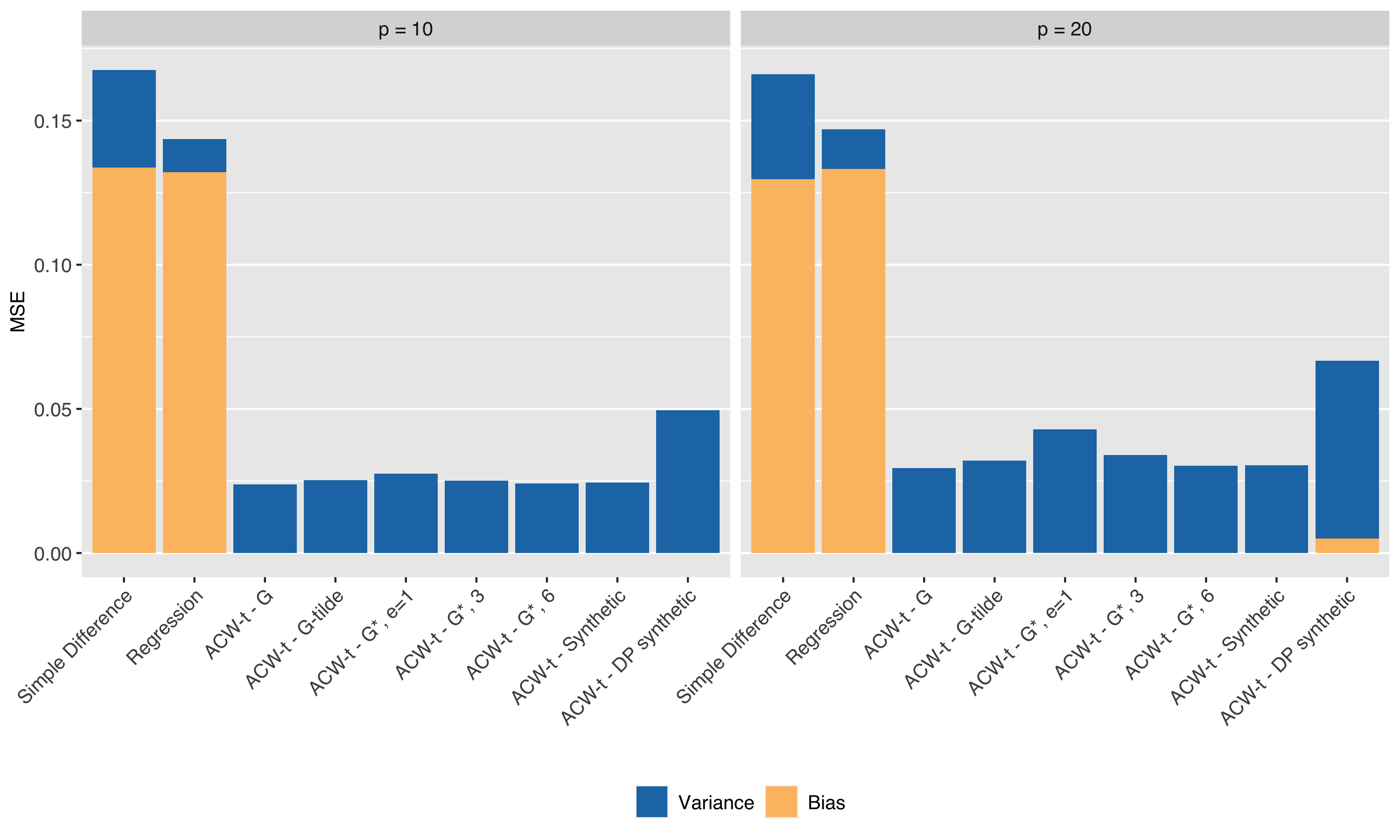
Figure 2: MSE calculated across 1,000 iterations for estimators of the PATE for different numbers of covariates ($p$). The MSE is decomposed into the squared bias and the variance of the estimator. “Regression” indicates the regression estimator with only RCT covariates ${\hat{\tau}^{OLS}({\bm{X}}_{\{i\in\mathcal{R}\}})}$. “ACWT-t $[\cdot]$” indicates the augmented calibration weighted estimator ${\hat{\tau}^{ACW-t}}(\cdot)$. “G” is a gram matrix of the auxiliary data (${\bm{G}}$), “G-tilde” is the entry-wise noisy gram matrix (${\tilde{\bm{G}}}$), and “G*, e=1” is the differentially private gram matrix (${\bm{G}^{\ast}}$) with $\epsilon=1$. “Synthetic” and “DP synthetic” are vanilla and differentially private synthetic data (${\tilde{\bm{D}}},{\bm{D}^{\ast}}$).

We then generate the treatment assignment $T_{i}\sim\mbox{Bern}(.5)$ for the RCT sample, the observed outcomes $Y_{i}=T_{i}Y_{i}^{t}+(1-T_{i})Y_{i}^{c}$ and calculate the estimators. To compare the simple difference and regression estimators to a calibrated weighted estimator with more comparable variance, we calculate the augmented calibration weighted estimator ${\hat{\tau}^{ACW-t}}(\cdot)$ as described in Lee et al. (2021). The weights are estimated to calibrate the empirical mean of the RCT to the empirical mean of the auxiliary study $\hat{\mu}(\cdot)$. In the optimization problem (Equation 1), $\frac{1}{m}\sum_{i\in\mathcal{O}}g(\bm{X}_{i})=\hat{\mu}(\cdot)$. The weights are estimated by solving the optimization problem with Lagrange multipliers and Newton’s equation (see Lee et al., 2021, for more details). We adapt the genRCT package Yang (2021) code to calculate ${\hat{\tau}^{ACW-t}}(\cdot)$ in R. We additionally estimate a 95% confidence interval for each estimator. We use the standard estimators for the simple difference and regression estimators and the bootstrap estimator suggested by Lee et al. (2021) with 100 bootstraps for the ${\hat{\tau}^{ACW-t}}(\cdot)$ estimator.

Figure 2 shows the empirical MSE for each estimator, estimated across the 1,000 simulations. We note that the results displayed for the DP synthetic data with $p=20$ are based on 500 simulations because the algorithm could not find a solution to the calibration weights in 50% of the simulations. Blue represents the variance component of MSE and orange represents the squared bias component of the MSE. The simple difference and regression estimators, which only rely on data from the RCT have large estimated MSEs, which are primarily due to large squared biases, as compared to little or no bias of ${\hat{\tau}^{ACW-t}}(\cdot)$. Due to the shift in the distribution of $X^{S}$ in the RCT sample, the average SATE across simulations is .86, which larger than the true PATE of .5. The simple difference and regression estimators are unbiased for the SATE, so they are upwardly biased for the PATE in this case. ${\hat{\tau}^{ACW-t}}(\cdot)$ performs similarly across different disclosure limiting transformations of the auxiliary data. The differentially private auxiliary mean vector even with a small privacy budget, corresponding to high levels of privacy, perform similarly to the original auxiliary data when $p=10$. The exception is the differentially private synthetic data, which has larger variance and shows a small amount of bias when $p=20$.

	Coverage
Estimator of $\tau_{PATE}$	$p=10$	$p=20$
RCT only
${\hat{\tau}^{DM}}$	0.50	0.53
${\hat{\tau}^{OLS}({\bm{X}}_{\{i\in\mathcal{R}\}})}$	0.10	0.13
Include auxiliary data
${\hat{\tau}^{ACW-t}}({\bm{G}})$	0.95	0.96
${\hat{\tau}^{ACW-t}}({\tilde{\bm{G}}}),\lambda=1$	0.93	0.96
${\hat{\tau}^{ACW-t}}({\bm{G}^{\ast}}),\epsilon=1$	0.94	0.89
${\hat{\tau}^{ACW-t}}({\bm{G}^{\ast}}),\epsilon=3$	0.95	0.94
${\hat{\tau}^{ACW-t}}({\bm{G}^{\ast}}),\epsilon=6$	0.95	0.96
${\hat{\tau}^{ACW-t}}({\tilde{\bm{D}}})$	0.95	0.97
${\hat{\tau}^{ACW-t}}({\bm{D}^{\ast}}),\epsilon=3$	0.87	0.69

Table 1: Estimated coverage probability of the PATE for 95% confidence intervals across 1,000 iterations. 95% confidence intervals are estimated with 100 boostrap samples for ${\hat{\tau}^{ACW-t}}(\cdot)$. ${\hat{\tau}^{DM}}$ and ${\hat{\tau}^{OLS}({\bm{X}}_{\{i\in\mathcal{R}\}})}$ are the simple difference and regression estimators, respectively. ${\bm{G}}$ is a gram matrix of the auxiliary data, ${\tilde{\bm{G}}}$ and ${\bm{G}^{\ast}}$ are the element-wise noisy and differentially private gram matrices, and ${\tilde{\bm{D}}}$ and ${\bm{D}^{\ast}}$ are vanilla and differentially private synthetic data, respectively.

Table 1 shows the empirical coverage probability of the true PATE (.5) for 95% confidence intervals, across the 1,000 simulations. The regression estimator has very poor coverage for the PATE, as does the simple difference estimator, which only has higher coverage because the variance is larger. The coverage of bootstrap 95% confidence intervals for the calibration weighted estimator is close to .95 cross the different disclosure limiting transformations of the auxiliary data, with the exception of ${\bm{G}^{\ast}}$ (differentially private gram matrix) when $\epsilon=1$ and $p=10$ and the differentially private synthetic data. There is also a steep drop-off in coverage when $p=20$ versus $p=10$ when leveraging the differentially private synthetic data in ${\hat{\tau}^{ACW-t}}(\cdot)$.

To summarize, when the PATE is the estimand of interest, leveraging auxiliary data in the analysis of an RCT with ${\hat{\tau}^{ACW-t}}(\cdot)$ can greatly reduce the MSE of the treatment effect estimate, and this continues to be true when using auxiliary data that has undergone disclosure limiting transformations.

4.2 Improving Experimental Precision

In the second simulation study, the goal is to estimate the average treatment effect for an RCT sample. We assume that there is an RCT evaluating a specific treatment, and a related observational study which includes the outcome of interest. We do not necessarily observe the treatment in the auxiliary observational study. However, given that observational studies typically have large sample sizes, we can expect to get good estimates of model parameters for a model of the outcome on observed covariates, resulting in good predictions of the outcome. Further, if there are a large number of covariates, an observational study will likely better estimate model parameters for all covariates than a small RCT. As discussed in Section 2.2, predictions of the outcome based on a model trained on the auxiliary data can therefore be a very powerful covariate to include in RCT covariate adjustment. For simplicity, we consider a setting where the RCT and observational samples arise from the same, linear, data generating model (there is no covariate shift) and where the regression models match this data generating model. There are other covariate adjustment methods incorporating auxiliary data that account for covariate shift (see Appendix B).

We emulate a hypothetical RCT with $n=100$ and an auxiliary (observational) study with $m=1,000$. For both studies, we generate ${\bm{x}_{i}}$ from i.i.d $N(\bm{0},\bm{I}_{p})$ distributions. Then, $Y_{i}^{c}=.5+\beta^{\prime}{\bm{X}_{i}}+\varepsilon_{i}$, where $\varepsilon_{i}\sim N(0,.3)$. To make some covariates contribute to the outcome, while others are noise, .6 of the elements of $\bm{\beta}_{1\times p}$ are $\sqrt{.7/(.6p)}$, while the rest are set to 0. By this data generating process, $\mathbb{V}[Y_{i}^{c}]=1$, and the proportion of variance explained by the covariates is .7. We let $\tau_{SATE}=.5$, so $Y_{i}^{t}=Y_{i}^{c}+.5$ under the constant treatment effect assumption. In the auxiliary study, we assume that there is no treatment, so $Y_{i}=Y_{i}^{c}$ for $i\in\mathcal{O}$.

We calculate each disclosure limiting transformation of the auxiliary data as described in the previous section. With each transformation of the auxiliary data, we fit an OLS model of the outcome on the covariates. For each of these models, we predict the outcome for subjects in the RCT ($i\in\mathcal{R}$). Denote this prediction ${\hat{Y}_{i}(\cdot)}$, so $\hat{Y}_{i}({\bm{G}})$ is the prediction of the outcome for subject $i$ based on the model fit with ${\bm{G}}$. Let ${\hat{\bm{Y}}_{\mathcal{O}}}({\bm{G}})$ denote the $n\times 1$ length vector of these predictions for the RCT subjects. The auxiliary study is set aside.

Next, we estimate the variance of the comparison estimators. Since we are interested in the average treatment effect for an RCT sample, we treat the outcomes and covariates as fixed. We then generate 1,000 treatment assignment vectors $T_{i}\sim\mbox{Bern}(.5),i\in\mathcal{R}$. For each treatment assignment vector we generate the observed outcomes and calculate each estimator: ${\hat{\tau}^{DM}}$, ${\hat{\tau}^{OLS}({\bm{x}}_{\{i\in\mathcal{R}\}})}$, and ${\hat{\tau}^{OLS}({\hat{\bm{Y}}_{\mathcal{O}}(\cdot)})}$ for each disclosure limiting transformation. Because $n=100$, the regression estimator fit only on the RCT covariates, ${\hat{\tau}^{OLS}({\bm{x}}_{\{i\in\mathcal{R}\}})}$, runs into dimensionality issues as $p$ grows. Therefore, we allow a maximum of 20 RCT covariates to be included in the regression model. With $p=50$, we choose 20 covariates that have a non-zero coefficient in the data generating model, emulating analyses of the RCT using variable selection and/or expert knowledge that would select predictive covariates.

We calculate the empirical variance of the estimates across the 1,000 treatment assignment vectors. Finally, we calculate empirical relative efficiency as compared to the estimators only relying on RCT data: ${\hat{\tau}^{DM}}$, ${\hat{\tau}^{OLS}({\bm{x}}_{\{i\in\mathcal{R}\}})}$ by dividing the empirical variance of ${\hat{\tau}^{DM}}$ and ${\hat{\tau}^{OLS}({\bm{x}}_{\{i\in\mathcal{R}\}})}$ respectively by the empirical variance of each estimator.

Regression Estimator

Covariates

RCT only

none ($\hat{\tau}^{DM}$)

${\bm{x}_{i}},i\in\mathcal{R}$

Include auxiliary data

$\hat{Y}_{i}({\bm{G}})$

$\hat{Y}_{i}({\tilde{\bm{G}}}),\lambda=1$

$\hat{Y}_{i}({\bm{G}^{\ast}}),\epsilon=1$

$\hat{Y}_{i}({\bm{G}^{\ast}}),\epsilon=3$

$\hat{Y}_{i}({\bm{G}^{\ast}}),\epsilon=6$

$\hat{Y}_{i}({\bm{G}^{\ast}}),\epsilon=10$

$\hat{Y}_{i}({\bm{G}^{\ast}}),\epsilon=15$

$\hat{Y}_{i}({\tilde{\bm{D}}})$

$\hat{Y}_{i}({\bm{D}^{\ast}}),\epsilon=3$

$p=10$
Var($\hat{\tau}$)	REDM	RER
0.041	1.0	0.3
0.014	3.0	1.0
0.013	3.3	1.1
0.014	3.0	1.0
0.015	2.8	0.9
0.013	3.1	1.0
0.013	3.2	1.1
0.013	3.2	1.1
0.013	3.2	1.1
0.013	3.2	1.1
0.038	1.1	0.4

$p=20$
Var($\hat{\tau}$)	REDM	RER
0.040	1.0	0.4
0.015	2.7	1.0
0.012	3.3	1.2
0.015	2.7	1.0
0.022	1.9	0.7
0.016	2.6	1.0
0.014	2.9	1.1
0.013	3.0	1.1
0.013	3.1	1.2
0.013	3.1	1.2
0.039	1.0	0.4

$p=50$
Var($\hat{\tau}$)	REDM	RER
0.041	1.0	0.7
0.027	1.5	1.0
0.013	3.2	2.1
0.018	2.3	1.5
0.041	1.0	0.7
0.040	1.0	0.7
0.028	1.5	1.0
0.021	2.0	1.3
0.018	2.3	1.5
0.017	2.5	1.6
0.041	1.0	0.7

Table 2: Estimated variance and relative efficiencies compared to the simple difference estimator (RE_DM) and regression estimator with RCT covariates (RE_R) across 100 data generations and 1,000 treatment assignments within each generation. The relative efficiency is calculated by dividing Var($\hat{\tau}$) for the simple difference estimator or regression estimator with RCT covariates by Var($\hat{\tau}$) for the estimator in the corresponding row. $\hat{Y}_{i}(\cdot)$ is a prediction of the outcome from a model fit on the auxiliary data. ${\bm{G}}$ is a gram matrix of the auxiliary data, ${\tilde{\bm{G}}}$ and ${\bm{G}^{\ast}}$ are the element-wise noisy and differentially private gram matrices. ${\tilde{\bm{D}}}$ and ${\bm{D}^{\ast}}$ are vanilla and differentially private synthetic data. $\lambda$ is the variance of the normal noise added to each element of $D$ to calculate ${\tilde{\bm{G}}}$. $\epsilon$ is the privacy budget for the differentially private transformations.

For each value of $p$, we implement the above 100 times (100 data generations). Finally, we average the estimated variance and relative efficiencies of each estimator across the 100 data generations. These results are displayed in Table 2. Relative efficiencies greater than 1 indicate that the corresponding estimator is more precise than the simple difference or regression estimator, while relative efficiencies less than 1 indicate the opposite.

When the number of covariates included in covariate adjustment is small ($p=10$), all of estimators incorporating covariates are more precise that the simple difference estimator. Using ${\hat{\bm{Y}}_{\mathcal{O}}(\cdot)}$ as a covariate in the regression estimator performs as well as using the RCT covariates for most disclosure limiting transformations of the auxiliary data. Since the regression model fit with the RCT was correctly specified for $p=10\mbox{ and }p=20$, we expected there to be only small gains in precision integrating the observational data. When $p=50$, the regression estimator fit on only the RCT covariates is limited in the number of predictive covariates that can be included in the modeling, so there are gains to using predictions fit on the auxiliary data. ${\hat{\tau}^{OLS}({\hat{\bm{Y}}_{\mathcal{O}}(\cdot)})}$ is more precise than ${\hat{\tau}^{OLS}({\bm{x}}_{\{i\in\mathcal{R}\}})}$ other than for differentially private transformations of the auxiliary data with $\epsilon=1$ and $\epsilon=3$. The differentially private synthetic data performs notably worse than the other covariate adjusted estimators, with comparable precision to the simple difference estimator.

When $p=10$, not much is lost when using the transformed versions of the auxiliary data rather than the original data - the variances of ${\hat{\tau}^{OLS}}({\hat{\bm{Y}}_{\mathcal{O}}(\cdot)})$ is similar across these estimators. Increasing the number of covariates, the adjusted estimator incorporating the transformed versions of the auxiliary data have higher variance than ${\hat{\tau}^{OLS}}(\hat{Y}_{i}({\bm{G}}))$. We can clearly see the privacy-utility trade-off, with the variance of ${\hat{\tau}^{OLS}}(\hat{Y}_{i}({\bm{G}^{\ast}}))$ decreasing as the privacy budget $\epsilon$ increases. The differentially private transformations loose utility faster as $p$ increases because the magnitude of noise added increases with $p^{2}$. The noise added to statistics to achieve differential privacy additionally depends on the sensitivity of the statistics to removing one observation from the data. This sensitivity decreases as $m$ increases, so the utility of ${\bm{G}^{\ast}}$ as a covariate would stay consistent with the utility of ${\bm{G}}$ as the size of the auxiliary study gets very large (see Appendix A).

As noted previously, these results are based on correctly specified regression models and RCT and auxiliary samples that arise from the same data generating process. In practice, neither of these assumptions may be true, and it can be preferred to use design-based estimators. See Appendix B for a discussion and simulations which show that these results hold with a design-based estimator that is robust to model mis-specification and covariate shift.

5 Discussion

In this paper, we presented disclosure limiting transformations of observational data that can be combined with experimental data to estimate the PATE and SATE. These disclosure limiting transformations included noise injected gram matrices (differentially private and entry-wise noise) and synthetic data (vanilla and differentially private). We found that leveraging these transformed versions of observational data to estimate the PATE greatly improved the MSE (and eliminated bias) as compared to methods using only the RCT data. We also found that transformed versions of auxiliary data could improve precision when estimating the SATE, beyond the precision achieved through covariate adjustment with RCT covariates alone.

There is little discussion of using the gram matrix of a data matrix as a disclosure limiting transformation in the literature, to the best of our knowledge. The gram matrix is a reasonable place to start for disclosure limiting transformations since it provides useful summary statistics of the data and some protection against disclosure, which can be augmented with additional random noise. The gram matrix supports some flexible model fitting – any outcome and covariates can be chosen out of the columns in the data matrix. Ridge and lasso regularized regression can be calculated in addition to standard OLS.

In addition to disclosure risk and utility, there are practical considerations that could be taken into account when choosing a disclosure limiting technique. For example computing time differed greatly between the transformations – generating differentially private synthetic data for 50 covariates and 1,000 observations took 30 minutes as compared to seconds for other transformations. Another important consideration is that the additional uncertainty introduced by privacy-transformations may be more challenging to communicate to data users for some techniques than for others. In the case of ${\bm{G}^{\ast}}$ and ${\tilde{\bm{G}}}$, the additional uncertainty is rather clear – we add noise with a certain distribution to the gram matrix, the variance of which is parameterized with a couple of parameters. On the other hand, estimating valid standard errors associated with synthetic data requires multiple replicates of the synthetic data and survey sampling methods.

We focus on a small set of disclosure limiting techniques for discussion’s sake. Further evaluation of disclosure limiting transformations and causal estimators would be valuable. For example, the inverse propensity score weighted estimator (IPSW) is an estimator of the PATE, which combines experimental and observational data Colnet et al. (2021). The IPSW estimator requires pooling experimental and observational data, and therefore requires subject-level data. Future work could evaluate the utility of different methods for synthetic data generation of observational data for use in the IPSW estimator.

Integrating observational and experimental data in treatment effect estimation is a powerful and exciting direction in causal inference. There is a lost opportunity when RCT analysts cannot access relevant observational data. On the other hand, individuals who provide their data have the right to control their information and expect that sensitive information will not be released to the public. In practice, choosing a tolerable disclosure risk, balanced with data utility, is a policy decision. In this paper, we present information to inform such a decision, illustrating the privacy-utility trade-off for different data privacy techniques when integrating private auxiliary data with experimental data for causal inference.

6 Code and Data

All code to replicate the simulations is available at https://github.com/manncz/exp-obs-priv.

7 Acknowledgements

The research reported here was supported by the Institute of Education Sciences, U.S. Department of Education, through Grant R305D210031 to the University of Michigan. The opinions expressed are those of the authors and do not represent views of the Institute or the U.S. Department of Education nor other funders. Charlotte Z. Mann was additionally supported by the National Science Foundation RTG grant DMS-1646108.

Appendix A Utility of Disclosure Limiting Transformations with Large Auxiliary Data

As the size of the auxiliary study ($m$) grows, there is less of a trade-off between privacy and utility for noisy versions of the gram matrix. The sensitivity of the gram matrix to changes in one observation gets smaller. Therefore, the magnitude of the noise necessary to achieve differential privacy for a specific privacy budget shrinks as $m\rightarrow\infty$. The difference between the original gram matrix and ${\tilde{\bm{G}}}$ will also shrink.

We ran the same simulation study as in Section 4.2, but with $m=10,000$ instead of $1,000$. The results are shown in Table 3, which can be compared with the results when $m=1,000$ (Table 2). Integrating disclosure limiting transformations of the auxiliary data now maintains essentially the same utility as using the original auxiliary data. Particularly, the variance of the estimators stays constant even as we decrease the privacy budget and increase the number of covariates for the differentially private procedure.

Regression Estimator

Covariates

RCT only

none ($\hat{\tau}^{DM}$)

${\bm{x}_{i}},i\in\mathcal{R}$

Include auxiliary data

$\hat{Y}_{i}({\bm{G}})$

$\hat{Y}_{i}({\tilde{\bm{G}}}),\lambda=1$

$\hat{Y}_{i}({\bm{G}^{\ast}}),\epsilon=1$

$\hat{Y}_{i}({\bm{G}^{\ast}}),\epsilon=3$

$\hat{Y}_{i}({\bm{G}^{\ast}}),\epsilon=6$

$\hat{Y}_{i}({\bm{G}^{\ast}}),\epsilon=10$

$\hat{Y}_{i}({\bm{G}^{\ast}}),\epsilon=15$

$\hat{Y}_{i}({\tilde{\bm{D}}})$

$p=10$
Var($\hat{\tau}$)	REDM	RER
0.040	1.0	0.3
0.013	3.1	1.0
0.012	3.3	1.1
0.012	3.3	1.1
0.012	3.3	1.1
0.012	3.3	1.1
0.012	3.3	1.1
0.012	3.3	1.1
0.012	3.4	1.1
0.012	3.3	1.1

$p=20$
Var($\hat{\tau}$)	REDM	RER
0.040	1.0	0.4
0.015	2.7	1.0
0.012	3.3	1.2
0.013	3.2	1.2
0.012	3.3	1.2
0.012	3.3	1.2
0.012	3.3	1.2
0.012	3.3	1.2
0.012	3.3	1.2
0.012	3.3	1.2

$p=50$
Var($\hat{\tau}$)	REDM	RER
0.040	1.0	0.7
0.027	1.5	1.0
0.012	3.3	2.2
0.013	3.1	2.1
0.013	3.1	2.0
0.013	3.2	2.1
0.012	3.3	2.2
0.012	3.3	2.2
0.012	3.3	2.2
0.013	3.2	2.1

Table 3: Estimated variance and relative efficiencies compared to the simple difference estimator (RE_DM) and regression estimator with RCT covariates (RE_R) across 100 data generations and 1,000 treatment assignments within each generation. The relative efficiency is calculated by dividing Var($\hat{\tau}$) for the simple difference esimator or regression estimator with RCT covariates by Var($\hat{\tau}$) for the estimator in the corresponding row. $\hat{Y}_{i}(\cdot)$ is a prediction of the outcome from a model fit on the auxiliary data. ${\bm{G}}$ is a gram matrix of the auxiliary data, ${\tilde{\bm{G}}}$ and ${\bm{G}^{\ast}}$ are the element-wise noisy and differentially private gram matrices, and ${\tilde{\bm{D}}}$ and ${\bm{D}^{\ast}}$ are vanilla and differentially private synthetic data.

Appendix B Design-Based Covariate Adjustment with Auxiliary Data

Using a prediction of the outcome as a covariate in the regression estimator is effective to reduce variance in experimental estimates when the model is correctly specified and there is no covariate shift between the RCT and auxiliary study. In practice, neither of these assumptions may be true. Design-based methods for covariate adjustment do not require modeling assumptions on top of those that are typically employed with design-based analysis of randomized experiments. The covariate adjusted estimator proposed by Gagnon-Bartsch et al. [2021] is robust to model mis-specification and accounts for possible covariate shift between the RCT and auxiliary study.

Gagnon-Bartsch et al. [2021] is part of the literature proposing residualizing the outcomes in the IPW estimator with some function of the covariates Robins et al. [1994], Scharfstein et al. [1999], Robins [2000], Aronow and Middleton [2013], Sales et al. [2018], Wu and Gagnon-Bartsch [2018]. In general, such adjusted estimators take the form:

$${\hat{\tau}^{fIPW}}=\frac{1}{n}\Big{[}\sum_{i\in\mathcal{R}}T_{i}\frac{Y_{i}-\hat{f}({\bm{x}_{i}})}{\pi}-(1-T_{i})\frac{Y_{i}-\hat{f}({\bm{x}_{i}})}{1-\pi}\Big{]}.$$

Authors have proposed different functions $f(\cdot)$ for adjustment. Aronow and Middleton [2013] remain agnostic to an exact choice for $f(\cdot)$, but note that the choice of $f(\cdot)$ could impact efficiency. Sales et al. [2018] use $f(\cdot)=y_{i}^{c}$ (so $\hat{f}({\bm{x}_{i}})$ estimates the control potential outcome for subject $i$). Wu and Gagnon-Bartsch [2018] propose $f(\cdot)=m_{i}=\pi y_{i}^{t}+(1-\pi)y_{i}^{c}$. $m_{i}$ is not observed, but if $\hat{f}({\bm{x}_{i}})=m_{i}$, ${\hat{\tau}^{fIPW}}=\tau^{SATE}$, minimizing the estimator’s variance. Therefore, the better $\hat{f}({\bm{x}_{i}})$ estimates $m_{i}$, the more precise ${\hat{\tau}^{fIPW}}$ will be.

Using auxiliary, observational data to estimate $f(\cdot)$ can further improve precision because the auxiliary data likely has a much larger sample size than the randomized experiment. Aronow and Middleton [2013], Sales et al. [2018] suggest using auxiliary data directly to estimate $f(\cdot)$, for example, letting $\hat{f}(\cdot)$ be a regression model fit on the auxiliary data. Gagnon-Bartsch et al. [2021] instead suggest using predictions of the outcome based on a regression model fit on the auxiliary data as a covariate to estimate $m_{i}$ in Wu and Gagnon-Bartsch [2018].

Like the regression estimator discussed in Section 2.2, Gagnon-Bartsch et al. [2021] only requires a model of the outcome of interest fit on the auxiliary data. We denote the specific variation of the adjusted IPW estimator in Gagnon-Bartsch et al. [2021] as ${\hat{\tau}^{SS}}(\cdot)$. We run the same simulations as in Section 4.2, using $\{\hat{Y}_{i}(\cdot),{\bm{x}_{i}}\}$ as covariates in the ensemble approach of ${\hat{\tau}^{SS}}(\cdot)$ instead of the regression estimator. The ensemble approach interpolates between a model using the RCT covariates, and a model using only the auxiliary prediction, so it is robust to covariate shift. We implement the estimator using the loop.estimator package in R Wu et al. [2022]. Table 4 shows that the adjusted IPW estimator ${\hat{\tau}^{SS}}(\cdot)$ performs equivalently to the regression estimator in this setting.

Estimator of $\tau_{SATE}$

RCT only

${\hat{\tau}^{DM}}$

${\hat{\tau}^{OLS}({\bm{x}}_{\{i\in\mathcal{R}\}})}$

Include auxiliary data

${\hat{\tau}^{SS}}({\bm{G}})$

${\hat{\tau}^{SS}}({\tilde{\bm{G}}}),\lambda=1$

${\hat{\tau}^{SS}}({\bm{G}^{\ast}}),\epsilon=1$

${\hat{\tau}^{SS}}({\bm{G}^{\ast}}),\epsilon=3$

${\hat{\tau}^{SS}}({\bm{G}^{\ast}}),\epsilon=6$

${\hat{\tau}^{SS}}({\bm{G}^{\ast}}),\epsilon=10$

${\hat{\tau}^{SS}}({\bm{G}^{\ast}}),\epsilon=15$

${\hat{\tau}^{SS}}({\tilde{\bm{D}}})$

${\hat{\tau}^{SS}}({\bm{D}^{\ast}}),\epsilon=3$

$p=10$
Var($\hat{\tau}$)	REDM	RER
0.041	1.0	0.3
0.014	3.0	1.0
0.013	3.3	1.1
0.014	3.0	1.0
0.015	2.8	0.9
0.013	3.1	1.0
0.013	3.2	1.1
0.013	3.2	1.1
0.013	3.2	1.1
0.013	3.2	1.1
0.026	1.6	0.5

$p=20$
Var($\hat{\tau}$)	REDM	RER
0.040	1.0	0.4
0.015	2.7	1.0
0.012	3.3	1.2
0.015	2.7	1.0
0.022	1.9	0.7
0.016	2.6	1.0
0.014	2.9	1.1
0.013	3.0	1.1
0.013	3.1	1.2
0.013	3.1	1.2
0.030	1.3	0.5

$p=50$
Var($\hat{\tau}$)	REDM	RER
0.041	1.0	0.7
0.027	1.6	1.0
0.013	3.3	2.1
0.018	2.3	1.5
0.037	1.1	0.7
0.037	1.1	0.7
0.028	1.5	1.0
0.021	2.0	1.3
0.018	2.3	1.5
0.017	2.5	1.6
0.037	1.1	0.7

Table 4: Estimated variance and relative efficiencies compared to the simple difference estimator (RE_DM) and regression estimator with RCT covariates (RE_R) across 100 data generations and 1,000 treatment assignments within each generation. The relative efficiency is calculated by dividing Var($\hat{\tau}$) for the simple difference estimator or regression estimator with RCT covariates by Var($\hat{\tau}$) for the estimator in the corresponding row. ${\bm{G}}$ is a gram matrix of the auxiliary data, ${\tilde{\bm{G}}}$ and ${\bm{G}^{\ast}}$ are the element-wise noisy and differentially private gram matrices, and ${\tilde{\bm{D}}}$ and ${\bm{D}^{\ast}}$ are vanilla and differentially private synthetic data.

References

- Colnet et al. [2021] Bénédicte Colnet, Imke Mayer, Guanhua Chen, Awa Dieng, Ruohong Li, Gaël Varoquaux, Jean-Philippe Vert, Julie Josse, and Shu Yang. Causal inference methods for combining randomized trials and observational studies: a review. arXiv:2011.08047 [stat], July 2021. URL http://arxiv.org/abs/2011.08047. arXiv: 2011.08047.
- Snoke and Bowen [2020] Joshua Snoke and Claire McKay Bowen. How Statisticians Should Grapple with Privacy in a Changing Data Landscape. CHANCE, 33(4):6–13, October 2020. ISSN 0933-2480. doi: 10.1080/09332480.2020.1847947. URL https://doi.org/10.1080/09332480.2020.1847947. Publisher: Taylor & Francis.
- Fellegi [1972] I. P. Fellegi. On the Question of Statistical Confidentiality. Journal of the American Statistical Association, 67(337):7–18, 1972. ISSN 0162-1459. doi: 10.2307/2284695. URL https://www.jstor.org/stable/2284695. Publisher: [American Statistical Association, Taylor & Francis, Ltd.].
- Raghunathan [2021] Trivellore E. Raghunathan. Synthetic Data. Annual Review of Statistics and Its Application, 8(1):129–140, 2021. doi: 10.1146/annurev-statistics-040720-031848. URL https://doi.org/10.1146/annurev-statistics-040720-031848.
- Schwartz [2013] Paul M Schwartz. The EU-U.S. Privacy Collision: A Turn to Institutions and Procedures. Harvard Law Review, 126(7):1966–2009, May 2013.
- Bellovin et al. [2018] Steven M. Bellovin, Preetam K. Dutta, and Nathan Reitinger. Privacy and Synthetic Datasets, August 2018. URL https://papers.ssrn.com/abstract=3255766.
- Wood et al. [2018] Alexandra Wood, Micah Altman, Aaron Bembenek, Mark Bun, Marco Gaboardi, James Honaker, Kobbi Nissim, David O’Brien, Thomas Steinke, and Salil Vadhan. Differential Privacy: A Primer for a Non-Technical Audience. SSRN Electronic Journal, 2018. ISSN 1556-5068. doi: 10.2139/ssrn.3338027. URL https://www.ssrn.com/abstract=3338027.
- Neyman et al. [1935] J. Neyman, K. Iwaskiewicz, and S. Kolodziejczyk. Statistical problems in agricultural experimentation (with discussion). Supplement to Journal of the Royal Statistical Society, 2:107–180, 1935.
- Rubin [1974] Donald B. Rubin. Estimating causal effects of treatments in randomized and nonrandomized studies. Journal of Educational Psychology, 66(5):688–701, 1974. ISSN 0022-0663. doi: 10.1037/h0037350. URL http://content.apa.org/journals/edu/66/5/688.
- Cole and Stuart [2010] Stephen R. Cole and Elizabeth A. Stuart. Generalizing evidence from randomized clinical trials to target populations: The ACTG 320 trial. American Journal of Epidemiology, 172(1):107–115, July 2010. ISSN 1476-6256. doi: 10.1093/aje/kwq084.
- Stuart et al. [2011] Elizabeth A. Stuart, Stephen R. Cole, Catherine P. Bradshaw, and Philip J. Leaf. The use of propensity scores to assess the generalizability of results from randomized trials. Journal of the Royal Statistical Society: Series A (Statistics in Society), 174(2):369–386, 2011. ISSN 1467-985X. doi: 10.1111/j.1467-985X.2010.00673.x. URL https://onlinelibrary.wiley.com/doi/abs/10.1111/j.1467-985X.2010.00673.x.
- Lesko et al. [2017] Catherine R. Lesko, Ashley L. Buchanan, Daniel Westreich, Jessie K. Edwards, Michael G. Hudgens, and Stephen R. Cole. Generalizing Study Results: A Potential Outcomes Perspective. Epidemiology (Cambridge, Mass.), 28(4):553–561, July 2017. ISSN 1531-5487. doi: 10.1097/EDE.0000000000000664.
- Dahabreh et al. [2019] Issa J. Dahabreh, Sarah E. Robertson, Eric J. Tchetgen, Elizabeth A. Stuart, and Miguel A. Hernán. Generalizing causal inferences from individuals in randomized trials to all trial-eligible individuals. Biometrics, 75(2):685–694, June 2019. ISSN 1541-0420. doi: 10.1111/biom.13009.
- Lee et al. [2021] Dasom Lee, Shu Yang, Lin Dong, Xiaofei Wang, Donglin Zeng, and Jianwen Cai. Improving trial generalizability using observational studies. Biometrics, pages 1–13, 2021. ISSN 1541-0420. doi: 10.1111/biom.13609. URL http://onlinelibrary.wiley.com/doi/abs/10.1111/biom.13609.
- Horvitz and Thompson [1952] D. G. Horvitz and D. J. Thompson. A Generalization of Sampling Without Replacement From a Finite Universe. Journal of the American Statistical Association, 47(260):663–685, 1952. ISSN 0162-1459. doi: 10.2307/2280784. URL http://www.jstor.org/stable/2280784. Publisher: [American Statistical Association, Taylor & Francis, Ltd.].
- Robins et al. [1994] James M. Robins, Andrea Rotnitzky, and Lue Ping Zhao. Estimation of Regression Coefficients When Some Regressors are not Always Observed. Journal of the American Statistical Association, 89(427):846–866, September 1994. ISSN 0162-1459. doi: 10.1080/01621459.1994.10476818. URL https://doi.org/10.1080/01621459.1994.10476818.
- Pocock [1976] S. J. Pocock. The combination of randomized and historical controls in clinical trials. Journal of Chronic Diseases, 29(3):175–188, March 1976. ISSN 0021-9681. doi: 10.1016/0021-9681(76)90044-8.
- Viele et al. [2014] Kert Viele, Scott Berry, Beat Neuenschwander, Billy Amzal, Fang Chen, Nathan Enas, Brian Hobbs, Joseph G. Ibrahim, Nelson Kinnersley, Stacy Lindborg, Sandrine Micallef, Satrajit Roychoudhury, and Laura Thompson. Use of historical control data for assessing treatment effects in clinical trials. Pharmaceutical statistics, 13(1):41–54, 2014. ISSN 1539-1604. doi: 10.1002/pst.1589. URL https://www.ncbi.nlm.nih.gov/pmc/articles/PMC3951812/.
- Aronow and Middleton [2013] Peter M. Aronow and Joel A. Middleton. A Class of Unbiased Estimators of the Average Treatment Effect in Randomized Experiments. Journal of Causal Inference, 1(1):135–154, May 2013. ISSN 2193-3685. doi: 10.1515/jci-2012-0009. URL http://www.degruyter.com/document/doi/10.1515/jci-2012-0009/html. Publisher: De Gruyter.
- Deng et al. [2013] Alex Deng, Ya Xu, Ron Kohavi, and Toby Walker. Improving the sensitivity of online controlled experiments by utilizing pre-experiment data. In Proceedings of the sixth ACM international conference on Web search and data mining - WSDM ’13, page 123, Rome, Italy, 2013. ACM Press. ISBN 978-1-4503-1869-3. doi: 10.1145/2433396.2433413. URL http://dl.acm.org/citation.cfm?doid=2433396.2433413.
- Gui [2020] George Gui. Combining Observational and Experimental Data Using First-stage Covariates. arXiv:2010.05117 [econ, stat], December 2020. URL http://arxiv.org/abs/2010.05117. arXiv: 2010.05117.
- Opper [2021] Isaac M. Opper. Improving Average Treatment Effect Estimates in Small-Scale Randomized Controlled Trials. Technical report, Annenberg Institute at Brown University, January 2021. URL https://www.edworkingpapers.com/ai21-344. Publication Title: EdWorkingPapers.com.