Entanglement and Rényi entropies of (1+1)-dimensional O(3) nonlinear sigma model with tensor renormalization group

Abstract

We investigate the entanglement and Rényi entropies for the (1+1)-dimensional O(3) nonlinear sigma model using the tensor renormalization group method. The central charge is determined from the asymptotic scaling properties of both entropies. We also examine the consistency between the entanglement entropy and the $n$th-order Rényi entropy with $n\rightarrow 1$.

1 Introduction

In the past decade the tensor renormalization group (TRG) method , which was originally proposed in the condensed matter physics Levin:2006jai , has been getting applied to the particle physics. Although the target models in the initial stage were restricted to the 2$d$ ones, recent studies cover various four-dimensional (4$d$) models with the scalar, gauge and fermion fields Akiyama:2019xzy ; Akiyama:2020ntf ; Akiyama:2021zhf ; Akiyama:2020soe ; Akiyama:2022eip ; Akiyama:2023hvt . So far much attention has been paid to the sign-problem-free nature of the TRG method Shimizu:2014uva ; Shimizu:2014fsa ; Kawauchi:2016xng ; Kawauchi:2016dcg ; Yang:2015rra ; Shimizu:2017onf ; Takeda:2014vwa ; Kadoh:2018hqq ; Kadoh:2019ube ; Kuramashi:2019cgs ; Nakayama:2021iyp . On the other hand, there are few studies focusing on an ability of the direct evaluation of the partition function or the path-integral itself, which potentially allows us to measure the entanglement entropy ($S_{A}$) and $n$th-order Rényi entropy ($S_{A}^{(n)}$). Up to know only 2$d$ Ising and XY models were investigated Ueda_2014 ; Yang:2015rra ; Bazavov:2017hzi . Note that it is difficult for the Monte Carlo method to measure the entanglement and Rényi entropies so that recent lattice QCD studies focused on the so-called entropic $C$-function, which is an UV-finite observable in proportion to $\partial_{L}S^{(2)}_{A}(L)$ with $L$ an interval of length, avoiding the direct measurement of the entanglement and Rényi entropies Buividovich:2008kq ; Itou:2015cyu ; Rabenstein:2018bri .

In this paper we measure the entanglement and Rényi entropies of the (1+1)$d$ O(3) nonlinear sigma model (O(3) NLSM) using the density matrix without resort to the transfer matrix formalism employed in Ref. Bazavov:2017hzi . This model is massive and shares the property of asymptotic freedom with the (3+1)$d$ non-Abelian gauge theories. We extarct the central charge from the entanglement and $n$th-order Rényi entropies using the scaling formula for the non-critical (1+1)$d$ models Calabrese:2004eu . The value of the central charge is comapred with the previous result obtained from the entanglement entropy with the matrix product state (MPS) method Bruckmann:2018usp . We also make a consistency check between the entanglement and Rényi entropies by extrapolating the $n$th-order Rényi entropy to $n=1$.

This paper is organized as follows. In Sec. 2, we define the (1+1)$d$ O(3) NLSM on the lattice and give the tensor network representation. We present the numerical results for the entanglement and Rényi entropies in Sec. 3. We determine the central charge and discuss the consistency between the entanglement and Rényi entropies. Section 4 is devoted to summary and outlook.

2 Formulation and numerical algorithm

Although the definition of the (1+1)$d$ O(3) NLSM and its tensor network representation are already given in the appendix of Ref. Luo:2022eje , we briefly give the relevant expressions for this work to make this paper self-contained.

2.1 (1+1)-dimensional O(3) nonlinear sigma model

We consider the partition function of the O(3) NLSM on an isotropic hypercubic lattice $\Lambda_{1+1}=\{(n_{1},n_{2})\ |n_{1}=1,\dots,2L,n_{2}=1,\dots,N_{t}\}$ whose volume is $V=(2L)\times N_{t}$. The lattice spacing $a$ is set to $a=1$ unless necessary. A real three-component unit vector $\bm{s}(n)$ resides on the sites $n$ and satisfies the periodic boundary conditions $\bm{s}(n+{\hat{\nu}}L)=\bm{s}(n)$ ($\nu=1,2$). The lattice action $S$ is defined as

$$S = -\beta\sum_{n\in\Lambda_{1+1},\nu}\bm{s}(n)\cdot\bm{s}(n+{\hat{\nu}}).$$ (1)

The partition function $Z$ is given by

$$Z=\int{\cal D}[\bm{s}]e^{-S},$$ (2)

where ${\cal D}[\bm{s}]$ is the O(3) Haar measure, whose expression is given later.

2.2 Tensor network representation of the model

The vector $\bm{s}(n)$ in the model can be expressed as

$$\begin{array}[]{c}\bm{s}^{T}(\Omega)=(\cos\theta,\sin\theta\cos\phi,\sin\theta\sin\phi)\\ \Omega=(\theta,\phi)\quad,~{}\theta\in(0,\pi],~{}\phi\in(0,2\pi].\end{array}$$ (3)

The partition function and its measure are written as

$$Z =\int{\cal D}\Omega\prod_{n,\nu}e^{\beta\sum_{i=1}^{3}s_{i}(\Omega_{n})s_{i}(\Omega_{n+\hat{\nu}})},$$ (4)

$${\cal D}\Omega =\prod_{p=1}^{V}\frac{1}{4\pi}\sin(\theta_{p})d\theta_{p}d\phi_{p}~{}.$$ (5)

We discretize the integration (4) with the Gauss-Legendre quadrature Kuramashi:2019cgs ; Akiyama:2020ntf after changing the integration variables:

$$-1\leq\alpha = \frac{1}{\pi}\left(2\theta-\pi\right)\leq 1,$$ (6)

$$-1\leq\beta = \frac{1}{\pi}\left(\phi-\pi\right)\leq 1.$$ (7)

We obtain

$$Z=\sum_{\{\Omega_{1}\},\cdots,\{\Omega_{V}\}}\left(\prod_{n=1}^{V}\frac{\pi}{8}\sin(\theta(\alpha_{a_{n}}))w_{a_{n}}w_{b_{n}}\right)\prod_{\nu}M_{\Omega_{n},\Omega_{n+\hat{\nu}}}$$ (8)

with $\Omega_{n}=(\theta(\alpha_{a_{n}}),\phi(\beta_{b_{n}}))\equiv(a_{n},b_{n})$, where $\alpha_{a_{n}}$ and $\beta_{b_{n}}$ are $a$- and $b$-th roots of the $K$-th Legendre polynomial $P_{K}(s)$ on the site $n$, respectively. $\sum_{\{\Omega_{n}\}}$ denotes $\sum_{a_{n}=1}^{K}\sum_{b_{n}=1}^{K}$. $M$ is a 4-legs tensor defined by

$$M_{a_{n},b_{n},a_{n+\hat{\nu}},b_{n+\hat{\nu}}}=\exp\left\{\beta\sum_{i=1}^{3}s_{i}(a_{n},b_{n})s_{i}(a_{n+\hat{\nu}},b_{n+\hat{\nu}})\right\}~{}.$$ (9)

The weight factor $w$ of the Gauss-Legendre quadrature is defined as

$$w_{a_{n}}=\frac{2(1-{\alpha_{a_{n}}}^{2})}{K^{2}P^{2}_{K-1}({\alpha_{a_{n}}})},\quad w_{b_{n}}=\frac{2(1-{\beta_{b_{n}}}^{2})}{K^{2}P^{2}_{K-1}({\beta_{b_{n}}})}.$$ (10)

After performing the singular value decomposition (SVD) on $M$:

$$M_{a_{n},b_{n},a_{n+\hat{\nu}},b_{n+\hat{\nu}}}\simeq\sum_{i_{n}=1}^{D_{\text{cut}}}U_{a_{n},b_{n},i_{n}}(\nu)\sigma_{i_{n}}(\nu)V^{\dagger}_{i_{n},a_{n+\hat{\nu}},b_{n+\hat{\nu}}}(\nu),$$ (11)

where $U$ and $V$ denotes unitary matrices and $\sigma$ is a diagonal matrix with the singular values of $M$ in the descending order. We can obtain the tensor network representation of the O(3) NLSM on the site $n\in\Lambda_{1+1}$

$$T_{x_{n},x^{\prime}_{n},y_{n},y^{\prime}_{n}} =\frac{\pi}{8}\sqrt{\sigma_{x_{n}}(1)\sigma_{x^{\prime}_{n}}(1)\sigma_{y_{n}}(2)\sigma_{y^{\prime}_{n}}(2)}\sum_{a_{n},b_{n}}w_{a_{n}}w_{b_{n}}$$

$$\quad\times V^{\dagger}_{x_{n},a_{n},b_{n}}(1)U_{a_{n},b_{n},x^{\prime}_{n}}(1)V^{\dagger}_{y_{n},a_{n},b_{n}}(2)U_{a_{n},b_{n},y^{\prime}_{n}}(2),$$ (12)

where $D_{\text{cut}}$ is the bond dimension of tensor $T$, which controls the numerical precision in the TRG method. The tensor network representation of partition function is given by

$$Z\simeq\sum_{x_{0}x^{\prime}_{0}y_{0}y^{\prime}_{0}\cdots}\prod_{n\in\Lambda_{1+1}}T_{x_{n}x^{\prime}_{n}y_{n}y^{\prime}_{n}}={\rm Tr}\left[T\cdots T\right]~{}.$$ (13)

We employ the higher order tensor renormalization group (HOTRG) algorithm PhysRevB.86.045139 to evaluate $Z$.

2.3 Calculation of entanglement and Rényi entropies

Figure 1 illustrates the calculation procedure of the entanglement entropy. We divide the system to two subsystems A and B, both of which have the same lattice size with $L\times N_{t}$. The density matrix of subsystem A is defined by $\rho_{A}={1\over Z}{\rm Tr}_{B}[T\cdots T]$, where ${\rm Tr}_{B}$ denotes the trace restricted to the subsystem B. We use HOTRG to approximate the density matrix of subsystem A, in which $\rho_{A}\simeq{1\over Z}{\rm Tr}_{B}T_{xx^{\prime}y_{B}y^{\prime}_{B}}T_{x^{\prime}xy_{A}y^{\prime}_{A}}=M_{y_{A},y^{\prime}_{A}}$. The entanglement entropy is obtained by

$$S_{A}=-{\rm Tr}_{A}\rho_{A}\log(\rho_{A}).$$ (14)

Figure 2 depicts the calculation procedure of the $n$th-order Rényi entropy defined by

$$S_{A}^{(n)}=\frac{\ln{\rm Tr}_{A}\rho_{A}^{n}}{1-n},$$ (15)

where $\rho_{A}^{n}$ can be calculated by just computing the $n$th matrix power of $\rho_{A}$.

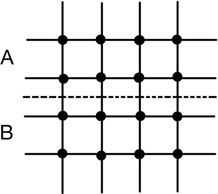
(a) Divide the system to two subsystems A and B.

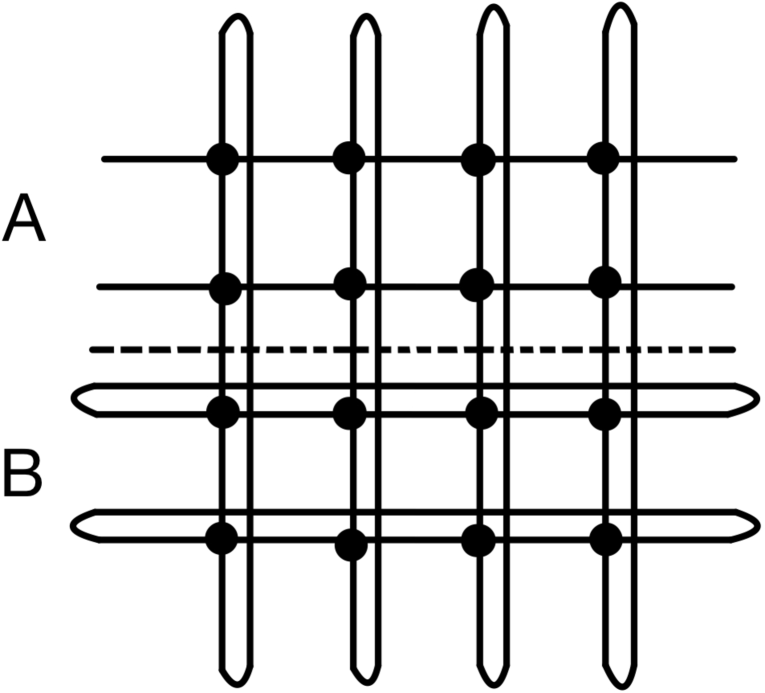
(b) Trace all legs for subsystem B.

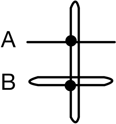
(c) Figure 1 is coarse-grained to this with HOTRG.

Figure 1: Calculation of entanglement entropy.

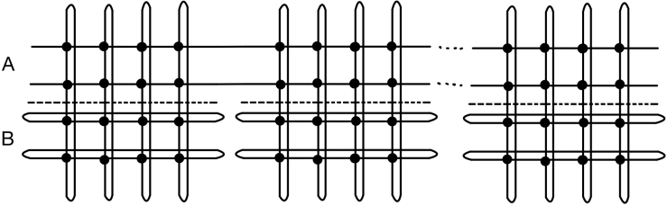
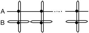
(a) Graphical representation of $n$th-order Rényi entropy $\rho_{A}^{(n)}$.

(b) Figure 2 is coarse-grained to this with HOTRG.

Figure 2: Calculation of $n$th-order Rényi entropy.

3 Numerical results

The density matrix $\rho_{A}$ is evaluated using HOTRG with the bond dimension $D_{\rm cut}\in[10,130]$. Note that the correlation length $\xi$ in this model was precisely measured over the range of $1.4\leq\beta\leq 1.9$ with the interval of $\Delta\beta=0.1$ in Ref. Wolff:1989hv . We list the values of $\xi$ in Table 1 for later convenience. In order to keep the condition $a\ll\xi\ll L$, our results are restricted to $1.4\leq\beta\leq 1.7$  in the following.

Figure 3 shows the $N_{t}$ dependence of the entanglement entropy $S_{A}(L)$ at $\beta=1.5$ with $L=128$, where the correlation length is expected to be $\xi\sim 11$ Wolff:1989hv . The degeneracy of the results for $S_{A}(L)$ with $N_{t}=256$, 512 and 1024 indicates the convergence of $S_{A}(L)$ in terms of $N_{t}$ so that $N_{t}=1024$ is large enough to be regarded as the zero temperature limit. In Fig. 4 we plot $S_{A}(L)$ with $N_{t}=1024$ at $\beta=1.4$, 1.5, 1.6 and 1.7. The entanglement entropy shows plateau behavior once the interval $L$ goes beyond the correlation length. This is an expected behavior under the condition of $\xi\ll L$ Calabrese:2004eu . As $\xi$ increases for larger $\beta$, the plateau of $S_{A}(L)$ starts at larger $L$ and its value is increased according to the theoretical expectation of $S_{A}(L)\sim\frac{c}{3}\ln\xi$ Calabrese:2004eu . In Fig. 5 we plot $S_{A}(L=128)$ at $\beta=1.4$, 1.5, 1.6 and 1.7 as a function of $1/D_{\rm cut}$. The data of $S_{A}(L=128)$ shows increasing trend, while slightly fluctuating, for vanishing $1/D_{\rm cut}$. This kind of fluctuation is commonly observed in the TRG method. See, e.g., Fig. 11 in Ref. Ueda_2014 for the Ising model with the HOTRG algorithm. The solid lines express the linear extrapolation of $S_{A}(L=128)$ at $1/D_{\rm cut}\leq 0.02$ to obtain the value at $D_{\rm cut}\rightarrow\infty$, which are listed in Table 1.

The mass gap $m$ in the (1+1)$d$ O(3) NLSM is expressed as Hasenfratz:1990zz

$$m=\frac{8}{e}\Lambda_{\overline{\rm MS}}=64\Lambda_{L}=\frac{128\pi}{a}\beta\exp\left(-2\pi\beta\right),$$ (16)

where the two-loop expression for the beta function at $\beta\rightarrow\infty$ is used in the last equation. Since the correlation length is inversely proportional to the mass gap the entanglement entropy is rewritten as

$$S_{A}=\frac{c}{3}\left(2\pi\beta-\ln\beta\right)+{\rm const.}$$ (17)

in terms of the coupling constant $\beta$. In Fig. 6 we plot the $\beta$ dependence of $S_{A}$ at $L=128$ with $N_{t}=1024$. We determine the central charge $c$ by fitting the data in the range of $1.4\leq\beta\leq 1.7$ with the function of Eq. (17), where the condition of $\xi\ll L$ is well satisfied. We obtain the value of $c=1.97(9)$, which is consistent with $c=2.04(14)$ obtained by the MPS method in Ref. Bruckmann:2018usp . We should also note that a recent study of the central charge for the 2$d$ classical Heisenberg model, which is equivalent to the (1+1)$d$ O(3) NLSM on the lattice, yields $c\sim 2$ with the tensor-network renormalization method Ueda_2022 . For an instructive purpose Fig. 7 shows an alternative plot of $S_{A}(L=128)$ with $N_{t}=1024$ as a function of $\xi$ measured in Ref. Wolff:1989hv . This is motivated by a concern that the (1+1)$d$ O(3) NLSM does not have a good asymptotic scaling property below $\beta\sim 2.0$ Wolff:1989hv ; Caracciolo:1994ud . The use of the fit function $S_{A}=\frac{c}{3}\ln\xi+{\rm const}.$ gives the central charge $c=2.15(3)$, which is consistent with $c=1.97(9)$ obtained above.

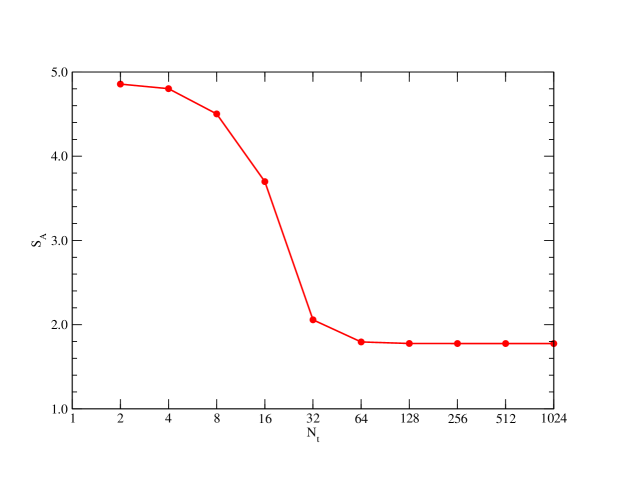
Figure 3: $N_{t}$ dependence of entanglement entropy at $\beta=1.5$. The bond dimension is $D_{\rm cut}=130$.

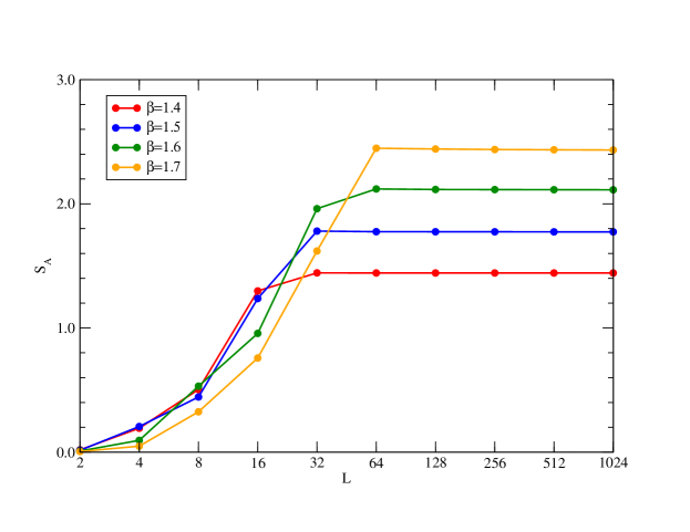
Figure 4: $L$ dependence of entanglement entropy with $N_{t}=1024$ at $\beta=1.4$, 1.5, 1.6 and 1.7. The bond dimension is $D_{\rm cut}=130$.

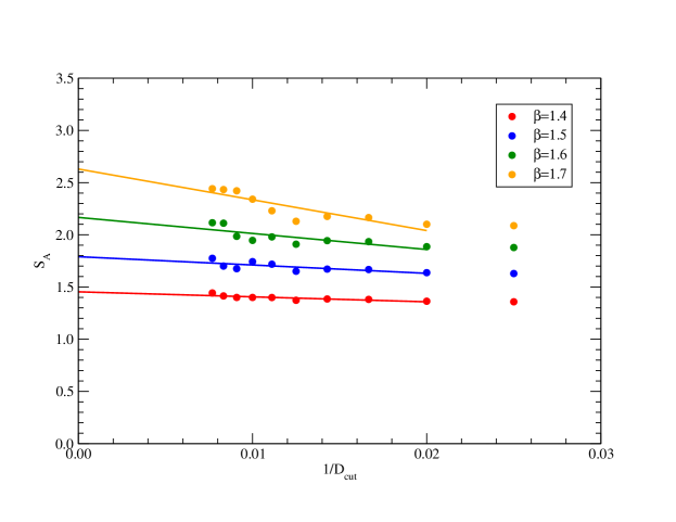
Figure 5: $1/D_{\rm cut}$ dependence of $S_{A}(L=128)$ with $N_{t}=1024$ at $\beta=1.4$, 1.5, 1.6 and 1.7. Solid lines denote linear extrapolation.

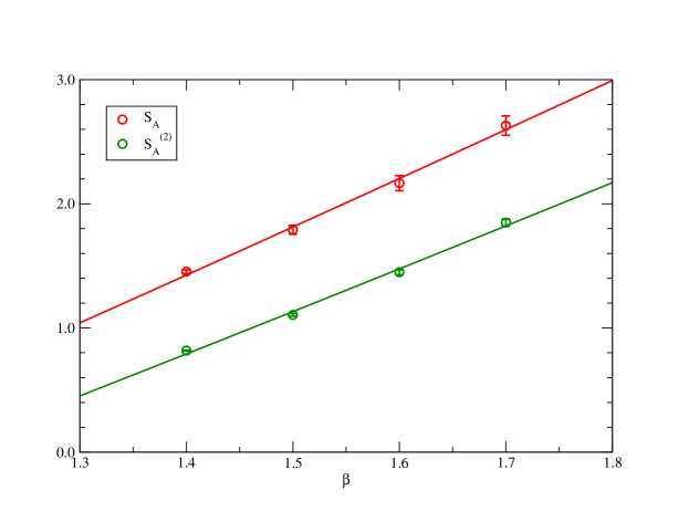
Figure 6: $\beta$ dependence of entanglement and 2nd-order Rényi entropies at $L=128$ with $N_{t}=1024$.

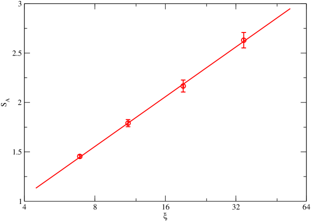
Figure 7: $\xi$ dependence of entanglement entropy at $L=128$ with $N_{t}=1024$.

Table 1: Results for $S_{A}(L=128)$ and $S_{A}^{(n)}(L=128)$ with $N_{t}=1024$ at $D_{\rm cut}\rightarrow\infty$. Values of correlation length $\xi$ are taken from Ref. Wolff:1989hv .

$\beta$	1.4	1.5	1.6	1.7
$\xi$	6.90(1)	11.09(2)	19.07(6)	34.57(7)
$S_{A}$	1.45(2)	1.79(4)	2.16(6)	2.63(8)
$S_{A}^{(1/2)}$	2.39(8)	2.68(14)	3.06(17)	3.63(17)
$S_{A}^{(2)}$	0.818(4)	1.105(11)	1.449(21)	1.849(30)
$S_{A}^{(3)}$	0.639(3)	0.878(8)	1.176(15)	1.535(22)
$S_{A}^{(4)}$	0.569(2)	0.784(7)	1.054(14)	1.338(19)
$S_{A}^{(5)}$	0.533(2)	0.735(7)	0.989(13)	1.299(18)
$S_{A}^{(6)}$	0.521(2)	0.705(7)	0.950(12)	1.247(17)
$S_{A}^{(7)}$	0.498(2)	0.686(6)	0.923(12)	1.213(17)
$S_{A}^{(8)}$	0.488(2)	0.672(6)	0.904(17)	1.188(17)
$S_{A}^{(9)}$	0.480(2)	0.662(6)	0.890(11)	1.170(16)
$S_{A}^{(10)}$	0.474(2)	0.653(6)	0.879(11)	1.155(16)
$S_{A}^{(11)}$	0.469(2)	0.647(6)	0.870(11)	1.144(16)

Now let us turn to the Rényi entropy. In Fig. 8 we plot the $N_{t}$ dependence of the 2nd-order Rényi entropy $S_{A}^{(2)}(L)$ at $\beta=1.5$ with $L=128$. As in Fig. 3 the plateau behavior of $S_{A}^{(2)}(L)$ is observed in the large $N_{t}$ region so that $N_{t}=1024$ is essentially regarded as the zero temperature limit of $S_{A}^{(2)}(L)$. Figure 9 compares $S_{A}^{(2)}(L)$ at $\beta=1.4$, 1.5, 1.6 and 1.7 with $N_{t}=1024$ fixed. Our observation is consistent with the theoretical expectation that $S_{A}^{(2)}(L)$ should stay constant in the range of $L\gg\xi$ according to $S_{A}^{(2)}(L)\sim\frac{c}{6}(1+1/n)\ln\xi$ Calabrese:2004eu . In Fig. 10 we show $D_{\rm cut}$ dependence of $S_{A}^{(2)}(L=128)$ at $\beta=1.4$, 1.5, 1.6 and 1.7. The extrapolated value of $S_{A}^{(2)}(L=128)$ at $D_{\rm cut}\rightarrow\infty$ is obtained by the linear fit of the data in terms of $1/D_{\rm cut}$ with $1/D_{\rm cut}\leq 0.02$. The $\beta$ dependence of $S_{A}^{(2)}$ at $L=128$ with $N_{t}=1024$ is plotted in Fig. 6 together with $S_{A}$. We extract the central charge $c$ from the data in $1.4\leq\beta\leq 1.7$ employing the following fit function with $n=2$:

$$S_{A}^{(n)}=\frac{c}{6}\left(1+\frac{1}{n}\right)\left(2\pi\beta-\ln\beta\right)+{\rm const.}$$ (18)

The value of $c=2.27(16)$ is slightly larger than that determined from $S_{A}$.

We repeat the same calculation for other $n$th-order Rényi entropy. The $n$ dependence of the central charge $c$ is plotted in Fig. 11, where the error bar of the central charge originates from the $1/D_{\rm cut}$ extrapolation and the scaling fit with Eq. (18) for the Rényi entropy. We observe that the central value of $c$ seems to converge to $c=2$ as $n$ increases. Here we consider the error of the $n$th-order Rényi entropy stemming from the errors of the eigenvalues in the density matrix. Suppose ${\bar{S}}_{A}^{(n)}$ is the true $n$th-order Rényi entropy and ${\bar{\lambda}}_{j}$ denotes the true $j$th eigenvalue in the density matrix $\rho_{A}$ normalized as ${\rm Tr}_{A}\rho_{A}=1$:

$${\bar{S}}_{A}^{(n)}=\frac{1}{1-n}\ln{\rm Tr}_{A}\rho_{A}^{n}=\frac{1}{1-n}\ln\sum_{j}{\bar{\lambda}}_{j}^{n},$$ (19)

where we assume the descending order for the eigenvalue ${\bar{\lambda}}_{1}>{\bar{\lambda}}_{2}>{\bar{\lambda}}_{3},\cdots$. Introducing the error of ${\bar{\lambda}}_{j}$, which is expressed as $\delta_{j}$, the measured Rényi entropy may be written as

$$S_{A}^{(n)}=\frac{1}{1-n}\ln\sum_{j}\left({\bar{\lambda}}_{j}+\delta_{j}\right)^{n}\simeq\frac{1}{1-n}\ln\sum_{j}\left({\bar{\lambda}}_{j}^{n}+n\delta_{j}{\bar{\lambda}}_{j}^{n-1}\right).$$ (20)

Focusing on the error of the Rényi entropy we find

$$\delta S_{A}^{(n)} = \frac{1}{1-n}\frac{1}{\sum_{i}({\bar{\lambda}}_{i}^{n})}n\sum_{j}\delta_{j}{\bar{\lambda}}_{j}^{n-1}=\frac{n}{1-n}\sum_{j}\frac{\delta_{j}}{{\bar{\lambda}}_{j}}\frac{1}{\sum_{i}\left(\frac{{\bar{\lambda}}_{i}}{{\bar{\lambda}}_{j}}\right)^{n}},$$ (21)

$$|\delta S_{A}^{(n)}| < \frac{n}{|1-n|}\sum_{j}\frac{|\delta_{j}|}{{\bar{\lambda}}_{j}}\frac{1}{\sum_{i}\left(\frac{{\bar{\lambda}}_{i}}{{\bar{\lambda}}_{j}}\right)^{n}}<\frac{n}{|1-n|}\sum_{j}\frac{|\delta_{j}|}{{\bar{\lambda}}_{j}}\left(\frac{{\bar{\lambda}}_{j}}{{\bar{\lambda}}_{1}}\right)^{n}\rightarrow\frac{|\delta_{1}|}{{\bar{\lambda}}_{1}}\;\;(n\rightarrow\infty).$$ (22)

The error of the Rényi entropy is bounded by the relative error of the maximum eigenvalue of the density matrix in the large $n$ limit. This may explain the convergence behavior of the central charge toward $c=2$ observed in Fig. 11.

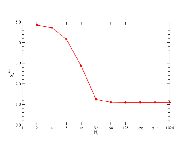
Figure 8: $N_{t}$ dependence of 2nd-order Rényi entropy at $\beta=1.5$. The bond dimension is $D_{\rm cut}=130$.

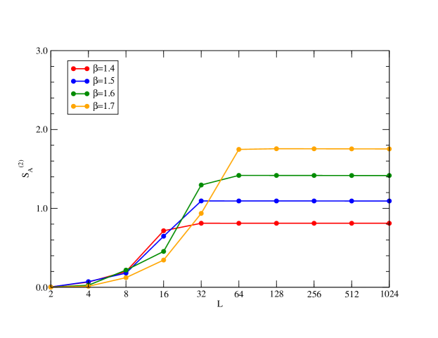
Figure 9: $L$ dependence of 2nd-order Rényi entropy with $N_{t}=1024$ at $\beta=1.4$, 1.5, 1.6 and 1.7. The bond dimension is $D_{\rm cut}=130$.

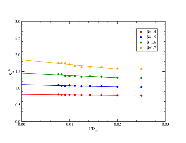
Figure 10: $1/D_{\rm cut}$ dependence of $S_{A}^{(2)}(L=128)$ with $N_{t}=1024$ at $\beta=1.4$, 1.5, 1.6 and 1.7. Solid lines denote linear extrapolation.

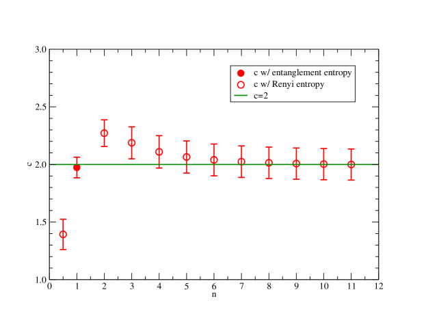
Figure 11: $n$ dependence of central charge $c$ obtained from $n$th-ordr Rényi (open) and entanglement (closed) entropies. Solid line denotes $c=2$ to guide your eyes.

In the Monte Carlo approach it is difficult to calculate the entanglement entropy. Actually, previous Monte Carlo studies on the (3+1)$d$ pure SU(N) gauge theories calculate the UV finite observable $\partial_{L}S^{(2)}_{A}(L)$ instead of $\partial_{L}S_{A}(L)$ assuming $S_{A}$ is close to $S_{A}^{(2)}$ Buividovich:2008kq ; Itou:2015cyu ; Rabenstein:2018bri . As observed in Fig. 6, the entanglement entropy shows sizable difference from the 2nd-order Rényi entropy. This fact implies that the extrapolation of the $n$th-order Rényi entropy to $n=1$ might be troublesome. It is worthwhile to check the $n$ dependence of the $n$th-order Rényi entropy and investigate how reliably we can extrapolate it to $n=1$. In Fig. 12 we plot the $n$-th order Rényi entropy as a function of $n$ together with the entanglement entropy at $n=1$. Note that $S_{A}^{(1/2)}$ is obtained by taking the square root of the density matrix. The dotted blue and green curves represent the fit results of the Rényi entropy at $n=2,...,5$ and $n=2,...,11$ employing the third and sixth order polynomial functions, respectively. The extrapolated value to $n=1$ shows sizable deviation from the directly measured entanglement entropy. It seems difficult to obtain the correct value of the entanglement entropy by an extrapolation of the $n$th order Rényi entropy at $n\geq 2$. On the other hand, the interpolations of the Rényi entropy at $n=1/2,2,...,4$ and $n=1/2,2,...,11$ with the third and sixth order polynomial functions, respectively, which are denoted by the pink and purple curves in Fig. 12, give consistent results with the entanglement entropy at $n=1$.

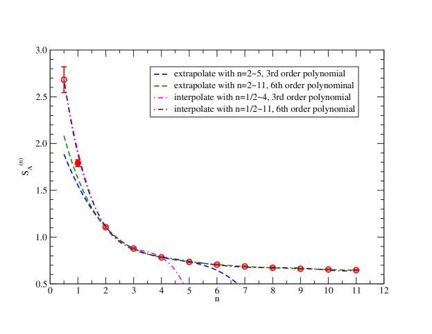
Figure 12: $n$ dependence of $n$th-order Rényi entropy with $N_{t}=1024$ at $\beta=1.5$. Solid symbol at $n=1$ denotes the entanglement entropy. All the results are extrapolated values at $D_{\rm cut}\rightarrow\infty$.

4 Summary and outlook

We have calculated the entanglement and Rényi entropies for the (1+1)-dimensional O(3) NLSM under the condition $\xi\ll L$ using the tensor renormalization group method. The central charge obtained from the asymptotic scaling behavior of the entanglement entropy is $c=1.97(9)$, which is consistent with $c=2.04(14)$ previously obtained with the MPS method. We have also investigated the consistency between the entanglement entropy and the Rényi entropies. The interpolation using $S_{A}^{(n)}$ at $n\geq 1/2$ gives a reasonable estimate for $S_{A}$ at $n=1$, while it is difficult to obtain $S_{A}$ at $n=1$ from the extrapolation of $S_{A}^{(n)}$ at $n\geq 2$. As a next step it would be interesting to check the area law in the (2+1)$d$ models.

- (1) M. Levin and C. P. Nave, Tensor renormalization group approach to two-dimensional classical lattice models, Phys. Rev. Lett. 99 (2007) 120601, [cond-mat/0611687].
- (2) Z. Y. Xie, J. Chen, M. P. Qin, J. W. Zhu, L. P. Yang and T. Xiang, Coarse-graining renormalization by higher-order singular value decomposition, Phys. Rev. B 86 (Jul, 2012) 045139, [1201.1144].
- (3) Y. Shimizu and Y. Kuramashi, Grassmann tensor renormalization group approach to one-flavor lattice Schwinger model, Phys. Rev. D90 (2014) 014508, [1403.0642].
- (4) R. Sakai, S. Takeda and Y. Yoshimura, Higher order tensor renormalization group for relativistic fermion systems, PTEP 2017 (2017) 063B07, [1705.07764].
- (5) D. Adachi, T. Okubo and S. Todo, Anisotropic Tensor Renormalization Group, Phys. Rev. B 102 (2020) 054432, [1906.02007].
- (6) D. Kadoh and K. Nakayama, Renormalization group on a triad network, 1912.02414.
- (7) S. Akiyama, Y. Kuramashi, T. Yamashita and Y. Yoshimura, Restoration of chiral symmetry in cold and dense Nambu–Jona-Lasinio model with tensor renormalization group, JHEP 01 (2021) 121, [2009.11583].
- (8) D. Adachi, T. Okubo and S. Todo, Bond-weighted tensor renormalization group, Phys. Rev. B 105 (Feb, 2022) L060402, [2011.01679].
- (9) S. Akiyama, Bond-weighting method for the Grassmann tensor renormalization group, 2208.03227.
- (10) S. Akiyama, Y. Kuramashi, T. Yamashita and Y. Yoshimura, Phase transition of four-dimensional Ising model with higher-order tensor renormalization group, Phys. Rev. D100 (2019) 054510, [1906.06060].
- (11) S. Akiyama, D. Kadoh, Y. Kuramashi, T. Yamashita and Y. Yoshimura, Tensor renormalization group approach to four-dimensional complex theory at finite density, JHEP 09 (2020) 177, [2005.04645].
- (12) S. Akiyama, Y. Kuramashi and Y. Yoshimura, Phase transition of four-dimensional lattice theory with tensor renormalization group, Phys. Rev. D 104 (2021) 034507, [2101.06953].
- (13) S. Akiyama and Y. Kuramashi, Tensor renormalization group study of (3+1)-dimensional 2 gauge-Higgs model at finite density, JHEP 05 (2022) 102, [2202.10051].
- (14) S. Akiyama and Y. Kuramashi, Critical endpoint of (3+1)-dimensional finite density gauge-Higgs model with tensor renormalization group, 2304.07934.
- (15) Y. Shimizu and Y. Kuramashi, Critical behavior of the lattice Schwinger model with a topological term at using the Grassmann tensor renormalization group, Phys. Rev. D90 (2014) 074503, [1408.0897].
- (16) H. Kawauchi and S. Takeda, Tensor renormalization group analysis of CP(-1) model, Phys. Rev. D93 (2016) 114503, [1603.09455].
- (17) H. Kawauchi and S. Takeda, Phase structure analysis of CP(N-1) model using Tensor renormalization group, PoS LATTICE2016 (2016) 322, [1611.00921].
- (18) L.-P. Yang, Y. Liu, H. Zou, Z. Xie and Y. Meurice, Fine structure of the entanglement entropy in the O(2) model, Phys. Rev. E 93 (2016) 012138, [1507.01471].
- (19) Y. Shimizu and Y. Kuramashi, Berezinskii-Kosterlitz-Thouless transition in lattice Schwinger model with one flavor of Wilson fermion, Phys. Rev. D97 (2018) 034502, [1712.07808].
- (20) S. Takeda and Y. Yoshimura, Grassmann tensor renormalization group for the one-flavor lattice Gross-Neveu model with finite chemical potential, PTEP 2015 (2015) 043B01, [1412.7855].
- (21) D. Kadoh, Y. Kuramashi, Y. Nakamura, R. Sakai, S. Takeda and Y. Yoshimura, Tensor network formulation for two-dimensional lattice = 1 Wess-Zumino model, JHEP 03 (2018) 141, [1801.04183].
- (22) D. Kadoh, Y. Kuramashi, Y. Nakamura, R. Sakai, S. Takeda and Y. Yoshimura, Investigation of complex theory at finite density in two dimensions using TRG, JHEP 02 (2020) 161, [1912.13092].
- (23) Y. Kuramashi and Y. Yoshimura, Tensor renormalization group study of two-dimensional U(1) lattice gauge theory with a term, JHEP 04 (2020) 089, [1911.06480].
- (24) K. Nakayama, L. Funcke, K. Jansen, Y.-J. Kao and S. Kühn, Phase structure of the CP(1) model in the presence of a topological -term, 2107.14220.
- (25) H. Ueda, K. Okunishi and T. Nishino, Doubling of entanglement spectrum in tensor renormalization group, Phys. Rev. B 89 (2014) 075116, [1306.6829].
- (26) A. Bazavov, Y. Meurice, S. W. Tsai, J. Unmuth-Yockey, L.-P. Yang and J. Zhang, Estimating the central charge from the Rényi entanglement entropy, Phys. Rev. D 96 (2017) 034514, [1703.10577].
- (27) P. V. Buividovich and M. I. Polikarpov, Numerical study of entanglement entropy in SU(2) lattice gauge theory, Nucl. Phys. B 802 (2008) 458–474, [0802.4247].
- (28) E. Itou, K. Nagata, Y. Nakagawa, A. Nakamura and V. I. Zakharov, Entanglement in Four-Dimensional SU(3) Gauge Theory, PTEP 2016 (2016) 061B01, [1512.01334].
- (29) A. Rabenstein, N. Bodendorfer, P. Buividovich and A. Schäfer, Lattice study of Rényi entanglement entropy in lattice Yang-Mills theory with , Phys. Rev. D 100 (2019) 034504, [1812.04279].
- (30) P. Calabrese and J. L. Cardy, Entanglement entropy and quantum field theory, J. Stat. Mech. 0406 (2004) P06002, [hep-th/0405152].
- (31) F. Bruckmann, K. Jansen and S. Kühn, O(3) nonlinear sigma model in 1+1 dimensions with matrix product states, Phys. Rev. D 99 (2019) 074501, [1812.00944].
- (32) X. Luo and Y. Kuramashi, Tensor renormalization group approach to (1+1)-dimensional SU(2) principal chiral model at finite density, Phys. Rev. D 107 (2023) 094509, [2208.13991].
- (33) U. Wolff, Asymptotic Freedom and Mass Generation in the O(3) Nonlinear Model, Nucl. Phys. B 334 (1990) 581–610.
- (34) S. Wang, Z.-Y. Xie, J. Chen, B. Normand and T. Xiang, Phase transitions of ferromagnetic potts models on the simple cubic lattice, Chinese Physics Letters 31 (jul, 2014) 070503.
- (35) P. Hasenfratz, M. Maggiore and F. Niedermayer, The Exact mass gap of the O(3) and O(4) nonlinear sigma models in d = 2, Phys. Lett. B 245 (1990) 522–528.
- (36) A. Ueda and M. Oshikawa, Tensor network renormalization study on the crossover in classical Heisenberg and RP2 models in two dimensions, Physical Review E 106 (jul, 2022) 014104.
- (37) S. Caracciolo, R. G. Edwards, A. Pelissetto and A. D. Sokal, Asymptotic scaling in the two-dimensional 0(3) sigma model at correlation length 10**5, Phys. Rev. Lett. 75 (1995) 1891–1894, [hep-lat/9411009].