Exploiting On-chip Heterogeneity of Versal Architecture for GNN Inference Acceleration

Abstract

Graph Neural Networks (GNNs) have revolutionized many Machine Learning (ML) applications, such as social network analysis, bioinformatics, etc. GNN inference can be accelerated by exploiting data sparsity in the input graph, vertex features, and intermediate data in GNN computations. For dynamic sparsity exploitation, we leverage the heterogeneous computing capabilities of AMD Versal ACAP architecture to accelerate GNN inference. We develop a custom hardware module that executes the sparse primitives of the computation kernel on the Programmable Logic (PL) and efficiently computes the dense primitives using the AI Engine (AIE). To exploit data sparsity during inference, we devise a runtime kernel mapping strategy that dynamically assigns computation tasks to the PL and AIE based on data sparsity. Our implementation on the VCK5000 ACAP platform leads to superior performance compared with the state-of-the-art implementations on CPU, GPU, ACAP, and other custom GNN accelerators. Compared with these implementations, we achieve significant average runtime speedup across various models and datasets of 162.42×, 17.01×, 9.90×, and 27.23×, respectively. Furthermore, for Graph Convolutional Network (GCN) inference, our approach leads to a speedup of 3.9-96.7× compared to designs using PL only on the same ACAP device.

I Introduction

Graph Neural Networks (GNNs) have become increasingly popular in recent years due to their ability to effectively learn from (unstructured) graph data. GNNs offer remarkable versatility and can be applied to a wide range of graph-related problems, including node classification [1], link prediction [2], graph classification [3], etc. This versatility has established GNNs as a powerful technique for various domains, such as computer vision [4], natural language processing [5], and recommendation systems [6], among others. In many practical applications [7], performing low-latency GNN inference is crucial for enabling real-time decision-making.

The computational characteristics of GNN inference present challenges for real-time applications, primarily due to the high computational complexity and the irregular memory access of graph data. CPUs are ill-suited for GNN acceleration [8] due to their sequential instruction-based architecture. On the other hand, GPUs excel at parallel processing and can accelerate GNNs. Still, they have limitations (e.g., complex cache hierarchy) in handling certain graph structures and memory access requirements [9]. To address these challenges, Field-Programmable Gate Arrays (FPGAs) offer a compelling solution. FPGAs provide flexibility [10, 11], programmability, and parallelism [12, 13, 14], making them well-suited for specific tasks such as message passing in GNN inference.

The Adaptive Compute Acceleration Platform (ACAP)[15] offers sequential instruction-based execution, parallel vector processing, and adaptive computing. Because GNN computation kernels can be mapped to sparse and dense primitives based on dynamic sparsity exploitation [16], ACAP offers a promising platform for accelerating GNN inference. The programmable logic (PL) component of ACAP can be leveraged to handle sparse primitives, while the AI Engine (AIE) are well suited to handle dense primitive. Nonetheless, there are several challenges in achieving efficient GNN acceleration using ACAP: (1) Developing an efficient hardware module for PL is crucial to accelerate sparse primitives effectively—this module must be carefully designed and optimized to maximize performance and resource utilization. (2) Although AI Engine exhibits high peak performance, achieving low-latency inference, using them can be a complex undertaking. Optimizing the utilization of the AI Engine and minimizing inference latency requires careful consideration of algorithmic optimizations to exploit the architectural features. (3) The interaction between PL and AIE must be designed efficiently to reduce data communication overhead. Effective data movement and synchronization mechanisms need to be implemented to facilitate seamless collaboration between the PL and AIE. The key contributions of this paper are:

• We develop an efficient accelerator design that leverages the heterogeneity of PL and AIE of the Versal architecture to accelerate GNN inference. The accelerator executes sparse primitives on PL and dense primitive on the AIE.

• We develop a runtime system that consists of a task analyzer and scheduler using the on-chip ARM processor that dynamically assigns computation tasks to the PL and AIE based on data sparsity.

• We evaluate the design on diverse datasets, including CiteSeer (CI), Cora (CO), PubMed (PU), Flickr (FL), NELL (NE), and Reddit (RE), for inference using state-of-the-art GNN models such as GCN, GraphSage, GIN, and SGC. The experimental results show that our implementation on VCK5000 achieves 162.42×, 17.01×, 9.90×, and 27.23× average speedup compared with the state-of-the-art CPU, GPU, ACAP, and other custom GNN accelerators, respectively.

The rest of the paper is organized as follows: Section II introduces the Background and Related work. In Section III, we demonstrate the intricate details of the Accelerator’s design. The evaluation results are presented in Section IV. Finally, we conclude the paper in Section V.

II Background and Related Work

II-A Background

II-A1 Graph Neural Networks

GNNs have been proposed for representation learning on graphs denoted as $\mathcal{G}(\mathcal{V},\mathcal{E})$. GNNs follow the message-passing paradigm (as outlined in Algorithm 1), where vertices recursively aggregate information from their neighbors. The last-layer embedding of the target vertex $v$ is denoted as $\bm{h}^{L}_{v}$. Typically, the Update() operation is implemented as a Multi-Layer Perceptron that transforms the vertex features. After the Aggregate() and Update() operations in each layer, an element-wise activation function is applied to the feature vectors. The output embedding $\bm{h}^{L}_{v}$ can be utilized for various downstream tasks, including node classification ([17, 18]), link prediction, and more. GCN [18], GraphSAGE [17], GIN [19], and SGC [20] are some representative GNN models.

Algorithm 1 GNN Computation Abstraction

1:Input graph: $\mathcal{G}(\mathcal{V},\mathcal{E})$; vertex features: $\left\{\bm{h}^{0}_{1},\bm{h}^{0}_{2},\bm{h}^{0}_{3},...,\bm{h}^{0}_{|\mathcal{V}|}\right\}$;

2:Output vertex features $\left\{\bm{h}^{L}_{1},\bm{h}^{L}_{2},\bm{h}^{L}_{3},...,\bm{h}^{L}_{|\mathcal{V}|}\right\}$;

3:for $l=1...L$ do

4:    for each vertex $v\in\mathcal{V}$ do

5:         $\bm{a}_{v}^{l}={\text{Update}(}\bm{h}_{v}^{l-1},\bm{W}^{l}\textbf{)}$

6:         $\bm{z}^{l}_{v}={\text{Aggregate}(}\bm{a}_{u}^{l}:u\in\mathcal{N}(v))$

7:         $\bm{h}_{v}^{l}=\sigma(\bm{z}_{v}^{l})$     

II-A2 Computation Kernels and Primitives in GNNs

The computation kernels involved in GNN inference consist of feature aggregation and feature transformation, corresponding to the Aggregate() and Update() operations in the message-passing paradigm of GNNs. These computation kernels can be mapped to fundamental computation primitives based on the data sparsity. These primitives include dense-dense matrix multiplication (GEMM), sparse-dense matrix multiplication (SpDMM), and sparse-sparse matrix multiplication (SpMM).

II-B Data Sparsity in GNN Inference

The density of a matrix is defined as the total number of non-zero elements divided by the total number of elements. Note that, the sparsity is given by $(1-\text{\emph{density}})$. The computation kernels in GNNs involve three types of matrices: graph adjacency matrix $\bm{A}$, vertex feature matrix $\bm{H}$, and weight matrix $\bm{W}$. The adjacency matrix $\bm{A}$ of different graph datasets [21] can have different densities. For a given adjacency matrix, different parts of the matrix can have different densities. For various graphs, the input feature matrices can have different densities. The feature matrices of different layers also have different densities. For the weight matrices, prior works [22, 23] have proposed various pruning techniques to reduce the density of the weight matrices. To leverage the above data sparsity, Zhang et al. [16] propose a technique called Dynasparse, which focuses on dynamically mapping computation kernels to primitives such as GEMM, SpDMM, and SpMM. The authors introduce a unified hardware architecture capable of supporting various primitives (GEMM, SpDMM, SpMM). This architecture offers different execution modes, each with distinct computation parallelism and the ability to skip zero-elements in the input matrix. Furthermore, the authors develop a runtime system that dynamically maps computation kernels to the appropriate primitives (to be executed on the unified architecture) using a performance model based on data sparsity. The performance model considers the trade-off between the computation parallelism and the ability to skip zero-elements of different execution modes, in order to reduce the inference latency. In this study, we extend the dynamic kernel-to-primitive mapping strategy from Dynasparse [16] to leverage the heterogeneous computing capabilities of the ACAP architecture for accelerating GNN inference. Specifically, for hardware mapping, we employ the AIE to execute the dense primitive (GEMM) due to its high peak performance. Additionally, we utilize the PL to construct a customized data path and memory organization, enabling efficient execution of sparse primitives (SpDMM, SpMM).

II-C Related Work

H-GCN[24] introduces a hybrid accelerator that leverages the heterogeneity of ACAP architecture by partitioning the input graph into subgraphs and assigning computations to either the AI Engine (AIE) or the Programmable Logic (PL) based on subgraph density. However, H-GCN’s graph partitioning and reordering approach can result in significant preprocessing overhead. In contrast, our work adopts a simple data partitioning strategy where we decompose the GNN kernel into different primitives (Section II-A2) and dynamically map them to the AIE or PL based on the data sparsity at runtime. This approach eliminates the need for complex graph partitioning and enables efficient execution of the GNN computations. The Dynasparse framework [16] presents a hardware-software codesign for accelerating GNN inference on data-center FPGAs. It encompasses offline compilation optimizations, a runtime system based on soft processors, and a PL-based accelerator design that exploits sparsity. In contrast, our work capitalizes on the heterogeneity of AMD ACAP devices, utilizing an ARM Cortex-A72 processor to execute a runtime system. Additionally, we employ both the PL and AIE components to execute GNN kernels mapping to different primitives of the GNN inference computations, leveraging the specific strengths of each component. Several existing works [25, 26, 27, 28, 29, 30, 31, 32, 33, 16, 34, 35, 36, 37, 38] have proposed FPGA-based acceleration techniques for GNN inference without AIE. These works typically employ custom compute hardware modules for operations such as SpMM, SpDMM, and GEMM on PL. In contrast, our work focuses on mapping onto the most suitable hardware components in ACAP to execute these compute kernels efficiently. By leveraging the capabilities of both PL and AIE, we enable efficient GNN inference on the ACAP platform.

III Accelerator Design

III-A Problem Definition

Our objective is to leverage the computational characteristics of the Programmable Logic - AI Engine, along with the Processor System (PS) of ACAP architecture, to accelerate full graph inference. Full graph inference involves performing the message-passing paradigm (as described in Algorithm 1) on the entire graph [26, 27, 28, 16]. This can be computationally demanding and memory-intensive, particularly for large graphs which do not fit on the on-chip memory.

To address this challenge, we propose an accelerator that effectively utilizes the on-chip heterogeneity of ACAP platform. By leveraging both the PL and AI Engine, our accelerator can efficiently accelerate GNN inference on datasets with varying degrees of sparsity. Note that our approach does not require generating an accelerator for each input graph and GNN model, thereby enhancing its efficiency and flexibility. For a given input graph and GNN model, initially stored on the host memory, we perform pre-processing (Section III-B) of the input graph and the GNN model on the host processor for hardware execution and transfer the processed input graph and GNN model to FPGA DDR.

III-B System Overview

Figure 1: System Overview

Figure 1 depicts the proposed design of leveraging ACAP architecture for dynamic sparsity exploitation (See Dynasparse [16]) in GNN inference. The architecture consists of three main parts: Application Processing Unit (APU), Programmable Logic (PL), and AI Engine (AIE) array. On PL, we implement multiple ALU (Arithmetic Logic Unit) arrays to execute sparse primitives (SpDMM, SpMM). The AIE array efficiently executes the dense primitive (GEMM) due to low-latency inter-tile communication and high computation density. The APU hosts a runtime system that dynamically maps kernels for execution. The host processor performs preprocessing for the input graph and GNN model. The board also has a high-performance communication infrastructure that efficiently interconnects computational and memory elements called Network on Chip (NoC). The input graph and the GNN model are stored in the host memory. After preprocessing, they are transferred to the FPGA DDR.

Preprocessing: For preprocessing, the host processor performs 2-D data partitioning [39], partitioning the input graphs into smaller submatrices along both dimensions to fit in the on-chip memory of ACAP, and enable parallel processing and efficient computation, for feature matrix $\bm{H}$, graph adjacency matrix $\bm{A}$, and weight matrix $\bm{W}$. We use $\bm{X}_{ij}$ to denote a partition of matrix $\bm{X}$.

Runtime: The runtime system consists of an analyzer and a scheduler. The analyzer dynamically maps the computation kernels (e.g., feature aggregation, feature transformation) to the basic primitives (GEMM, SpDMM, and SpMM) based on the data sparsity. As the AIE array is efficient for dense primitives and ALU arrays are efficient for sparse primitives, the analyzer uses a performance model to determine the kernel-to-primitive mapping and creates the tasks. Then, the scheduler adds the tasks to the task queues and dynamically schedules the tasks to ALU arrays and AIE array.

The following two sections elaborate on the hardware design and the runtime system. Figure 2 depicts the details of the proposed accelerator.

Figure 2: Overall Accelerator Design

III-C AI Engine (AIE) Array

The AI Engine Array is responsible for executing the dense-dense matrix multiplication (GEMM). Figure 2 provides an illustration of the organization of the AIE array specifically designed for GEMM execution. It consists of three main components: Buffer Tiles (BTs), Computation Cores (CCs), and Gather Tiles (GTs). To execute a GEMM operation $\bm{X}\times\bm{Y}$, the BTs load the input matrices, denoted as $\bm{X}$ and $\bm{Y}$, into their data memory from the DDR through the Direct Memory Access (DMA) engine. The loaded data is then transferred to the CCs. Communication between two consecutive kernels is established using a common buffer in the shared memory module [40]. Neighboring AI engine tiles can easily share data without memory transfers over DMA and AXI4-Stream interconnect by using the shared memory.

Figure 3: AI Engine Computation Core

AIE Computation Core (CC): Each AIE Computation Core (CC) consists of four AIE tiles. Each AIE tile is equipped with its own data memory module. The data flow involves transferring the data from the Buffer Tiles to the AIE Tiles. During each cycle, the vertex feature vectors are loaded into the AIE tile. The next step involves performing the Multiply-Accumulation (MAC) operation using the partial results obtained in the previous cycle. Figure 3 illustrates the computation process of executing the matrix multiplication $\bm{X}\times\bm{Y}$ on a Computation Core. Each matrix (e.g., $\bm{X}$, $\bm{Y}$) is evenly divided into four partitions. In each cycle, the $\bm{X}$ matrix is loaded in row-major order, and the $\bm{Y}$ matrix is loaded in column-major order into the respective CC. In the first cycle, the first row of matrix data is multiplied, and in the consequent cycles, subsequent rows are multiplied and accumulated with the previous product, as shown in the output matrix in Figure 3. The final output is sent to the Gather AIE Tiles to form the output matrix.

III-D Arithmetic Logic Unit (ALU) Array

The sparse primitives, specifically SpDMM and SpMM, are executed on the ALU Arrays, which are designed for efficient execution of sparse matrix multiplication. Figure 2 illustrates the architecture of the Arithmetic Logic Unit (ALU) Array. This array consists of $p$ computation pipelines, each comprising a Multiply Unit (MU) and an Accumulator Unit (AU). Each Multiply Unit contains an array of $q$ hardware multipliers, while each Accumulator Unit consists of an array of $q$ accumulators. Each Multiply unit and accumulator is instantiated as a Digital Signal Processing (DSP) slice on FPGA and value of $p$ and $q$ is restricted by the number of DSPs available. Additionally, the ALU Array incorporates three data buffers: BufferA, BufferG, and Result Buffer (RB). BufferA and BufferG are responsible for storing the two input matrices, denoted as $\bm{X}$ and $\bm{Y}$ respectively, while the Result Buffer stores the output matrix, $\bm{Z}$. To facilitate the routing of input data from BufferA and BufferG to the computation pipelines, each ALU Array includes a Pairing Unit. The Pairing Unit for each non-zero element in $\bm{X}$ from BufferA it fetches $q$ elements from BufferG. It effectively handles the irregular memory access patterns typically associated with sparse primitives. Furthermore, the ALU Array operates in two distinct execution modes: SpDMM mode and SpMM mode, dedicated to the execution of SpDMM and SpMM, respectively. The execution mode is set by the control bits of the ALU array. The overhead of switching execution modes is just one clock cycle.

Algorithm 2 SpDMM using Scatter-Gather Paradigm

1:Sparse matrix (BufferA): $\bm{X}$; Dense matrix (BufferG): $\bm{Y}$;

2:Output matrix (Result Buffer): $\bm{Z}$ ($\bm{Z}=\bm{X}\times\bm{Y}$);

3:while not done do

4:    for each $e(i,j,value)$ in $\bm{X}$ Parallel do $\triangleright$ Scatter Phase

5:         Fetch $\bm{Y}[i]$ from BufferG $\triangleright$ Pairing Unit

6:         Form input pair ($\bm{Y}[i]$, $e$) $\triangleright$ Pairing Unit     

7:    for each input pair Parallel do $\triangleright$ Gather Phase

8:         $u\leftarrow$Update($\bm{Y}[i],e.value$) $\triangleright$ Multiply Unit

9:         Fetch $\bm{Z}[j]$ from Result Buffer

10:         $\bm{Z}[j]\leftarrow$ Reduce($u$) $\triangleright$ Accumulator Unit     

SpDMM Mode: Multiplication of a sparse matrix with a dense matrix is executed using the Scatter-Gather Paradigm [16] shown in Algorithm 2. The sparse matrix denoted as $\bm{X}$ is stored in BufferU using the Coordinate (COO) format. The dense matrix denoted as $\bm{Y}$ is stored in BufferG. In SpDMM Mode the ALU array can execute upto $p\times q$ MAC operations per clock cycle.

Algorithm 3 SpMM using Row-wise Product

1:Sparse matrix (BufferA): $\bm{X}$; Sparse matrix (BufferG): $\bm{Y}$;

2:Output matrix (In Result Buffer): $\bm{Z}=\bm{X}\times\bm{Y}$;

3:for each row $\bm{Z}[j]$ in $\bm{Z}$ Parallel do

4:    Assign the workload of $\bm{Z}[j]$ to $(j\%p)^{\text{th}}$ pipeline

5:    for each $e(i,j,value)$ in $\bm{X}[j]$  do $\triangleright$ Scatter Phase

6:         Fetch $\bm{Y}[i]$ from BufferO $\triangleright$ Pairing Unit

7:         Form input pair ($\bm{Y}[i]$, $e$) $\triangleright$ Pairing Unit     

8:    for each input pair ($\bm{Y}[i]$, $e$) do $\triangleright$ Gather Phase

9:         for each non-zero $\bm{Y}[i][k]$ in $\bm{Y}[i]$ do

10:             Produce $u\leftarrow$ Update($e.value\times\bm{Y}[i][k]$)

11:             Merge $\bm{Z}[j][k]\leftarrow$ Reduce($u$)              

SpMM Mode: The multiplication of two input sparse matrices is executed using the Row-wise Product with Scatter-Gather paradigm as shown in Algorithm 3. For Row-wise Product, a row $\bm{Z}[j]$ of output matrix $\bm{Z}$ is calculated through:

$$\bm{Z}[j]=\sum_{i}\bm{X}[j][i]*\bm{Y}[i]\vspace{-3mm}$$ (1)

For calculating the output matrix $\bm{Z}$, a pipeline is assigned the workload of a row of output matrix (Equation 1). $p$ pipelines can calculate $p$ output rows in parallel until all the rows of the output matrices are calculated. SpMM Mode can execute $p$ multiply-accumulate (MAC) operations per clock cycle.

III-E Dynamic Task Management (Runtime System)

In the proposed accelerator design, the AIE array is efficient for dense primitives(GEMM), and the ALU array is efficient for sparse primitives(SpDMM, SpMM). To exploit various data sparsity in GNN inference, we implement a runtime system on APU that performs dynamic task management based on data sparsity.

Given a matrix multiplication $\bm{Z}=\bm{X}\times\bm{Y}$, we define a task as the process of calculating the partition of the large output matrix $\bm{Z}$. For example, for a partition $\{\bm{Z}_{ij}\}$, the task can be expressed as:

$$\bm{Z}_{ij}=\sum_{k}{\bm{X}_{ik}\times\bm{Y}_{kj}}\vspace{-2mm}$$ (2)

Therefore, each computation kernel (e.g., feature aggregation or feature transformation) can be decomposed into independent tasks. To execute these tasks efficiently, we dynamically schedule the tasks by analyzing the sparsity in the runtime system as shown in Algorithm 4.

Algorithm 4 Runtime System

1:Input graph $\mathcal{G}(\mathcal{V},\mathcal{E},\bm{X})$; GNN model with $L$ layers;

2:Output of GCN Inference;

3:$STQ\leftarrow\emptyset$ $\triangleright$ Sparse task queue

4:$DTQ\leftarrow\emptyset$ $\triangleright$ Dense task queue

5: ======= Analyzer ========

6:for $l=1$ to $L$ do $\triangleright$ Iterate each layer

7:    for  each kernel $kernel_{j}$ in layer $l$ do $\triangleright$ Iterate each kernel

8:         for each task $task_{k}$ in $kernel_{j}$ do

9:             $t_{\text{ALU}}=\mathcal{P}_{\text{ALU}}(task_{k})$

10:             $t_{\text{AIE}}=\mathcal{P}_{\text{AIE}}(task_{k})$

11:             if $t_{\text{ALU}}>t_{\text{AIE}}$ then

12:                 $STQ.push(task_{k})$

13:             else

14:                 $DTQ.push(task_{k})$                           

15: ======= Scheduler ========

16:while True do

17:    if there is an idle ALU array: $ALU_{i}$ then

18:         $task_{k}\leftarrow STQ.pop()$

19:         Execute $task_{k}$ on $ALU_{i}$     

20:while True do

21:    if AIE array is idle then

22:         $task_{k}\leftarrow DTQ.pop()$

23:         Execute $task_{k}$ on AIE array     

The runtime system consists of an Analyzer and a Scheduler. Moreover, the runtime system maintains two task queues – Sparse Task Queue (STQ) and Dense Task Queue (DTQ). For each task, the analyzer estimates its execution time on the ALU array and AIE array based on the theoretical performance model $\mathcal{P}_{\text{ALU}}()$ and $\mathcal{P}_{\text{AIE}}()$. Then, the analyzer adds the task to the Sparse Task Queue (STQ) or Dense Task Queue (DTQ) according to the estimated execution time. The scheduler schedules the tasks from the two task queues to the ALU arrays and AIE array.

Performance Model ($\mathcal{P}_{\text{ALU}}()$, $\mathcal{P}_{\text{AIE}}()$): The performance model (shown in Table I) estimates the execution cycle of each task. Based on the performance model, the Analyzer adds the task to the appropriate task queue. We define the density $\alpha_{\bm{X}}$ of a matrix $\bm{X}$ as the total number of non-zero elements divided by the total number of elements. For a given task (Equation 2), we use $\bm{X}_{i,:}$ to denote the concatenation of $\{\bm{X}_{ik}\}$ and use $\bm{Y}_{:,j}$ to denote the concatenation of $\{\bm{Y}_{kj}\}$. Then, the task (Equation 2) can be rewritten as:

$$\bm{Z}_{ij}=\bm{X}_{i,:}\times\bm{Y}_{:,j}\vspace{-1mm}$$ (3)

which has several properties w.r.t data sparsity, including the density of $\bm{X}_{i,:}$ denoted as $\alpha_{\bm{X}_{i,:}}$, and the density of $\bm{Y}_{:,j}$ denoted as $\alpha_{\bm{Y}_{:,j}}$. Suppose $\bm{X}_{i,:}\in\mathbb{R}^{m\times n}$ and $\bm{Y}_{:,j}\in\mathbb{R}^{n\times d}$. Using AIE array to execute this task, the task is treated as GEMM, and the total execution cycle is:

$$t_{\text{AIE}}=\frac{mnd}{f_{\text{AIE}}*N_{\text{AIE}}*\beta}$$ (4)

where $f_{\text{AIE}}$ is the frequency of AIE, $N_{\text{AIE}}$ is the total number of AIEs in the Computation Cores, and $\beta$ is the number of multiply-accumulate (MAC) operations that an AIE tile can perform each clock cycle. Using the ALU arrays to execute this task, the task is treated as SpDMM or SpMM, depending on which leads to lower execution cycle:

$$t_{\text{ALU}}=\min\left(\alpha_{\text{min}}\frac{mnd}{pq},\alpha_{\bm{X}_{i,:}}\alpha_{\bm{Y}_{:,j}}\frac{mnd}{p}\right)\times\frac{1}{\textit{f}_{\text{PL}}}$$ (5)

where $\alpha_{\text{min}}=\min(\alpha_{\bm{X}_{i,:}},\alpha_{\bm{Y}_{:,j}})$, and $\textit{f}_{\text{PL}}$ is the frequency of the ALU array.

Table I: Performance Model

	$\mathcal{P}_{\text{AIE}}()$	$\mathcal{P}_{\text{ALU}}()$
Primitives	GEMM	SpDMM	SpMM
MACs per Cycle	$N_{\text{AIE}}\times\beta$	$pq$	$p$
Execution cycles	$\frac{mnd}{N_{\text{AIE}}\times\beta}$	$\alpha_{\text{min}}\frac{mnd}{pq}$	$\alpha_{X}\alpha_{Y}\frac{mnd}{p}$
Frequency	$\textit{f}_{\text{AIE}}$	$\textit{f}_{\text{PL}}$	$\textit{f}_{\text{PL}}$

IV Experimental Results

IV-A Implementation Details

We implement the proposed accelerator on the AMD Xilinx Versal VCK5000 board. We use Verilog HDL to develop ALU arrays on PL and Vitis to develop Task Scheduler on APU [41] and AI Engine Compute Cores on AIEs. We integrate the complete system using Vitis. The Application Processing Unit (APU) - ARM Cortex-A72 runtime system uses C++ in AMD Xilinx Vitis Unified Software Platform (version 2021.2). For the AIE array, we implement 32 AIE CCs. Due to the limited on-chip memory, we implement 8 ALU arrays. In the performance model, each ALU array is configured with $p=8$ and $q=4$, determining the number of Multiply-Accumulate (MAC) operations per cycle. The resource utilization of the overall system is summarized in Table II. The ALU arrays, NoC, and AIE array operate at 297 MHz, 800 MHz, and 1 GHz, respectively. We develop a cycle-accurate simulator for our architecture design and runtime system (Algorithm 4) to obtain the hardware execution time. In the cycle-accurate simulator, Ramulator [42] is used to simulate the performance of DDR memory. Also, we use the host processor to execute the preprocessing steps (see Section III-B) and measure the preprocessing overhead.

Table II: Resource utilization of AIE and PL on VCK5000

	Tiles	AIE to NoC Interface	AIE to PL Interface
Overall AIE	192	16	32
Utilization	48%	100%	100%

	LUTS	DSPs	BRAMs	URAMs
Overall PL	776K	1024	880	400
Utilization	86.32%	52%	91%	86.4%

IV-B Experimental Setup

GNN Benchmarks: We evaluate the performance of our design on four well-known GNN models: GCN [18], GraphSage [17], GIN [19], and SGC [20].

Baselines: We compare the performance of our accelerator against state-of-the-art CPU, GPU, and GNN accelerators, including HyGCN [27], BoostGCN [28], Dynasparse [16], and H-GCN [24]. PyG and DGL are executed on Ryzen 3990x CPU and Nvidia RTX3090 GPU. Details of the platforms are shown in Table III.

Table III: Platform Specifications

Implementation	Platform	Frequency	DDR Memory Bandwidth
CPU	Ryzen 3990x	2.90 GHz	107 GB/s
GPU	Nvidia RTX3090	1.7 GHz	936.2 GB/s
HyGCN [27]	ASIC	1 GHz	256 GB/s
BoostGCN [28]	Stratix 10 GX	250 MHz	77 GB/s
Dynasparse [16]	Alveo U250	250 MHz	77 GB/s
ACAP	VCK 5000	297 MHz (PL) 1GHz (AIE)	102.4 GB/s

Datasets: We evaluate our design using several widely used datasets, including CiteSeer (CI) [18], Cora (CO) [18], PubMed (PU) [18], Flickr (FL) [43], NELL (NE) [44], and Reddit (RE) [17]. We evaluate with 2-layer GNNs in [18], [17], [19], and [20], where CI, CO, and PU have hidden layer dimensions of 16, while the hidden layer dimension of the remaining datasets is 128. Detailed dataset statistics are shown in Table IV.

Performance Metrics: We measure the hardware execution time, which represents the duration from when the accelerator starts scheduling computations until it generates the final results. We also measure the preprocessing time, which is the overhead of the data partitioning method (see Section III-B).

Table IV: Dataset Statistics

Dataset	Vertices	Edges	Features	Classes	Density of $\bm{A}$	Density of input $\bm{H}$
CO [18]	2708	5429	2708	7	0.14%	1.27%
CI [18]	3327	4732	3703	6	0.08%	0.85%
PU [18]	19717	44338	500	3	0.02%	10%
FL [43]	89,250	899,756	500	7	0.01%	46%
NE [44]	65,755	251,550	61278	186	0.0058%	0.01%
Re [17]	232,965	11$\times{10}^{7}$	602	41	0.21%	100%

Figure 4: Comparison of hardware execution time with state-of-the-art GNN accelerators

Table V: FLOPs and data count exploiting sparsity in feature matrices (FMs) and adjacency matrix (AM) for GCN inference. ”Sp. AM” refers to ”Sparsity in AM only,” and ”Sp. AM + FMs” to ”Sparsity in AM and FMs.” The FLOPs Reduction Factor refers to the ratio of FLOPs count when exploiting Sp. AM + FM to the scenario of Sp. AM only, while the Data Reduction Factor is the ratio for data count.

	CO	CI	PU	FL	NE	RE
#FLOPs Sp. AM	6.3E7	2.0E8	1.6E8	5.9E9	5.1E12	3.8E10
#FLOPs Sp. AM + FMs	1.2E6	2.1E6	1.8E7	2.8E9	5.3E10	3.7E10
FLOPs Reduction Factor	48.6$\times$	95.5$\times$	8.8$\times$	2.1$\times$	9.7$\times$	1.0$\times$
#Data Sp. AM	4.0E6	1.3E7	1.1E7	7.0E7	4.1E9	4.4E8
#Data Sp. AM + FMs	1.9E5	2.9E5	1.8E6	3.9E7	4.4E8	4.1E8
Data Reduction Factor	20.9$\times$	43.5$\times$	6.0$\times$	1.8$\times$	9.2$\times$	1.1$\times$

Table VI: Comparison of hardware execution time with state-of-the-art CPU, GPU, FPGA, and ACAP implementations. The values are in $ms$ and rounded to the nearest hundredth (The best results are in bold, and the second best results are underlined; OoM means out of GPU memory, and N/A means not available).

Model	Platform	Dataset
		CO	CI	PU	FL	NE	RE
GCN	PyG-CPU	2.10E+00	3.30E+00	8.70E+00	2.81E+02	1.54E+03	3.21E+04
	PyG-GPU	3.36E-01	3.76E-01	3.43E-01	7.02E+00	3.22E+01	OoM
	DGL-CPU	1.90E+00	7.70E+00	7.20E+00	3.58E+01	N/A	1.41E+02
	DGL-GPU	1.40E+00	1.40E+00	1.40E+00	2.10E+01	N/A	5.07E+01
	BoostGCN	2.90E-01	1.90E-02	1.60E-01	4.00E+01	N/A	1.90E+02
	HyGCN	3.00E-01	2.10E-02	6.40E+01	N/A	N/A	2.90E+02
	H-GCN	1.10E-01	2.90E-01	1.03E+00	1.02E+01	N/A	4.18E+01
	Dynasparse	4.70E-03	7.70E-03	6.30E-02	8.80E+00	2.90E+00	1.00E+02
	This paper	9.40E-03	1.22E-02	8.65E-02	6.10E+00	5.20E+00	9.10E+01
GraphSage	PyG-CPU	1.36E+01	2.81E+01	4.15E+01	3.36E+02	2.13E+04	OoM
	PyG-GPU	7.30E-01	1.43E+00	1.69E+00	1.78E+01	OoM	OoM
	DGL-CPU	3.42E+01	1.40E+01	2.43E+01	7.39E+01	N/A	3.39E+03
	DGL-GPU	8.61E-01	8.75E-01	8.37E-01	2.16E+01	N/A	4.45E+02
	Dynasparse	1.11E-01	3.34E-01	4.21E-01	1.91E+01	8.37E+02	3.31E+02
	This paper	1.01E-01	2.51E-01	1.95E-01	1.91E+00	5.07E+02	2.81E+02
GIN	PyG-CPU	1.26E+01	3.27E+01	4.14E+01	5.05E+02	1.91E+04	OoM
	PyG-GPU	6.80E-01	1.46E+00	1.22E+01	1.73E+01	OoM	OoM
	DGL-CPU	6.00E+00	2.28E+01	1.82E+01	1.52E+02	N/A	3.39E+03
	DGL-GPU	3.96E-01	4.30E-01	3.86E-01	1.95E+01	N/A	4.95E+02
	Dynasparse	1.08E-01	3.29E-01	3.71E-01	1.21E+01	8.37E+02	2.73E+02
	This paper	1.02E-01	2.52E-01	2.05E-01	7.61E+00	5.08E+02	2.94E+02
SGC	PyG-CPU	2.44E+01	5.63E+01	7.63E+01	1.27E+03	4.32E+04	OoM
	PyG-GPU	1.08E+00	2.50E+00	3.01E+00	3.32E+01	OoM	OoM
	DGL-CPU	N/A	N/A	N/A	N/A	N/A	N/A
	DGL-GPU	N/A	N/A	N/A	N/A	N/A	N/A
	Dynasparse	2.67E+00	8.70E-01	2.34E+00	1.27E+01	8.84E+02	5.05E+02
	This paper	1.22E-01	3.14E-01	3.18E-01	3.29E+00	7.82E+01	4.71E+02

IV-C Comparison with State-of-the-art

Comparison with prior implementation on ACAP: We compare the performance of our implementation with a prior implementation on the same platform, H-GCN [24]. Because we exploit data sparsity and utilize the heterogeneity of the platform and dynamically schedule the tasks to AIE and PL, we achieve an average of 9.9$\times$ speedup compared with H-GCN [24], as shown in Figure 4.

This speedup is due to our exploitation of matrix sparsity in all the computation kernels, including feature aggregation and feature update. In Table V, we provide a detailed analysis that shows a substantial reduction in both the number of floating-point operations (FLOPs) and the amount of data to be loaded, averaging 51$\times$ and 23.4$\times$, respectively, for the Planetoid datasets CO, CI, and PU. However, the reduction is comparatively smaller for FL and RE datasets (because the feature matrices of FL and RE have low sparsity. See Table IV), resulting in a smaller speedup compared with H-GCN.

Additionally, while H-GCN demonstrates faster hardware execution time on the Reddit dataset, our proposed approach significantly reduces the preprocessing overhead, as discussed in Section IV-E. Considering the end-to-end inference time, encompassing both the preprocessing overhead and the actual inference time, our method achieves a 6.6$\times$ speedup for the Reddit dataset.

Figure 5: Comparison of inference speedup over CPU and GPU (some speedups are not shown as those are OoM or N/A)

Comparison with CPU and GPU: We execute the same GNN models using state-of-the-art Pytorch Geometric (PyG) [45] and Deep Graph Library (DGL) [46] on a state-of-the-art CPU and GPU without exploiting data sparsity in feature matrix $\bm{H}$ and weight matrix $\bm{W}$. The results are shown in Figure 5; some results are not shown due to out of memory on the CPU/GPU. In summary, our implementation on ACAP achieves average speedup of 194.5$\times$, 12.9$\times$, 110.2$\times$, and 21.7$\times$ compared with PyG-CPU, PyG-GPU, DGL-CPU, and DGL-GPU, respectively. The achieved speedups are from exploiting the sparsity in GNN inference and the customized hardware architecture that can efficiently execute the sparse computation primitives (SpDMM, SpMM).

Comparison with GNN Accelerators: The speedup compared with the state-of-the-art accelerators is shown in Figure 4. The proposed design achieves an average speedup of 194.18$\times$ and 8.58$\times$ compared with HyGCN [27] and BoostGCN [28]. This is because our implementation utilizes the data sparsity in the vertex feature and input adjacency matrix, and AIE can efficiently execute the dense computation primitives (GEMM). We also compare our design with Dynasparse [16], which exploits data sparsity in GNN inference on FPGA. We achieve average speedup of 0.83$\times$, 2.90$\times$, 1.39$\times$, and 8.04$\times$ for GCN, GraphSage, GIN, and SGC models.

The hardware execution time is summarized in Table VI, where the fastest hardware execution time for various models and datasets is highlighted in bold, and the second fastest time is underlined. Our design achieves the best or second-best hardware execution time across all models and datasets.

Table VII: Hardware execution time on ACAP ($ms$) using PL only and using PL + AIE

Dataset	CO	CI	PU	FL	NE	RE
PL Only	2.45E-1	7.26E-1	6.55E-1	2.09E+1	5.02E+2	3.52E+2
PL + AIE	9.40E-3	1.22E-2	8.65E-2	6.10E+0	5.20E+0	9.10E+1

IV-D Exploring the heterogeneity of ACAP

Table VII compares the hardware execution time of the proposed accelerator design (PL + AIE) and the PL accelerator design (PL Only) for various datasets for GCN inference. The results highlight the significant speedup achieved by leveraging the heterogeneity of the ACAP device. On the average, the PL + AIE design achieves a speedup of 32.9$\times$ compared with the PL-only design. The improvement is due to the architecture of the AIE array that provides high parallelism when processing GEMM primitives, while the PL can efficiently compute the sparse primitives (SpDMM, SpMM).

Table VIII: Hardware execution time ($ms$) using various numbers of AIE tiles assuming sufficient external memory bandwidth. (192 and 384 are the number of AIE tiles used.)

Dataset	CO	CI	PU	FL	NE	RE
Current(192)	9.40E-3	1.22E-2	8.65E-2	6.10E+0	5.20E+0	9.10E+1
Scaled(384)	9.40E-3	1.22E-2	8.65E-2	2.53E+0	4.25E+0	7.97E+1

The board has limited external memory access bandwidth, so our current design uses only 32 AIE CCs (192 tiles). Increasing the number of AIE CCs will not proportionally increase the peak performance (# of AIE CCs * #MACs/cycle) as the computation would become memory bound. However, we simulate a scenario with double the AIE CCs, using 384 of 400 AIE tiles, assuming sufficient external memory access bandwidth to support all the AIE CCs. Table VIII shows that for the larger datasets (FL, NE, RE), increasing the number of tiles shows a speedup in hardware execution time. However, our hardware execution time on RE is still slower than H-GCN for RE as SpDMM dominates the overall performance on RE. While H-GCN utilizes AIEs to execute SpDMM, our approach uses PL only. Despite each ALU array being more efficient than one AIE CC at computing sparse primitives, the AIE has superior overall peak performance on SpDMM than PL-based design. Therefore, our hardware execution time is slower than H-GCN on RE dataset.

IV-E Analysis of Preprocessing and Runtime System Overhead

Preprocessing Overhead: We evaluate the overhead of preprocessing, detailed in Section III-B. This involves data partitioning on the host processor (Intel Xeon Gold CPU with 32 cores at 2.9 GHz) only once before the inference tasks start. The overhead of partitioning was smaller than the preprocessing time of the state-of-the-art GCN Accelerator on ACAP, H-GCN (which used Intel Xeon Gold with 56 CPU cores [24]). Figure 6 shows our speedups in preprocessing time.

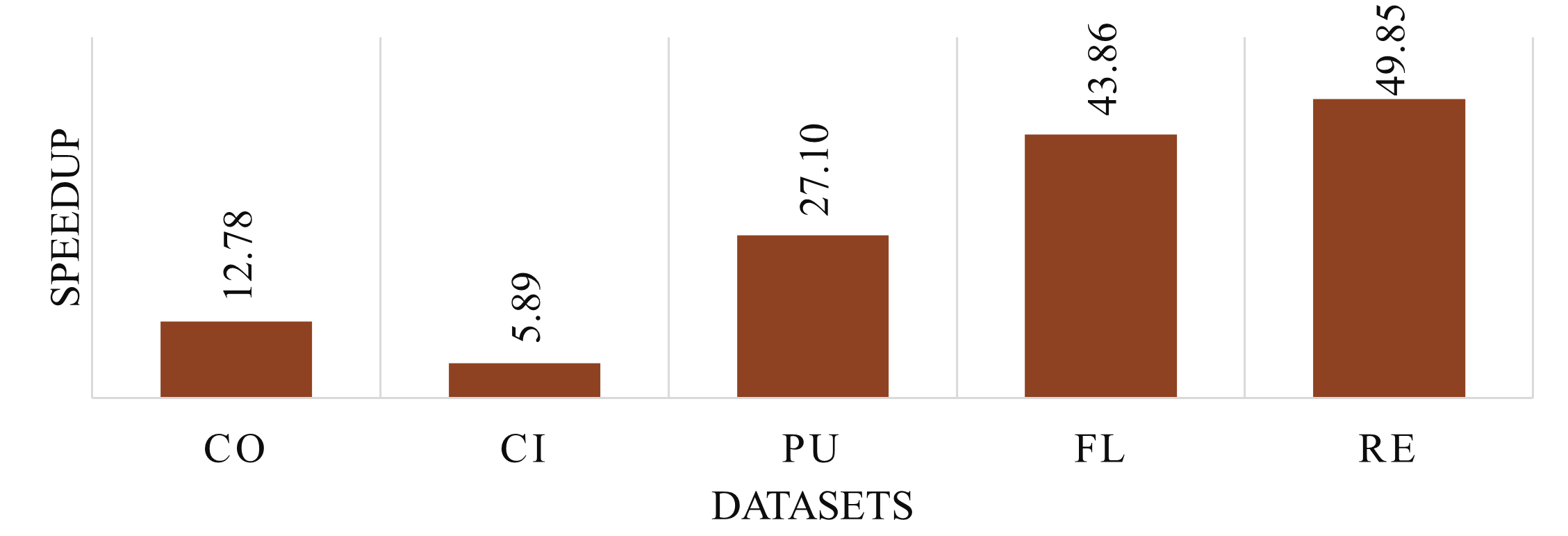
Figure 6: Comparison of preprocessing time with H-GCN [24]

Runtime System Overhead: The runtime system overhead corresponds to the execution time of Algorithm 4, performed on the Arm Cortex-A72 APU running at 1.7 GHz. After the initial tasks assignment, the runtime system overhead can be overlapped by concurrently analyzing and scheduling the tasks on AIE CCs and ALU arrays while they are working on the previously assigned tasks. The time it takes for the runtime system to analyze and schedule the initial tasks is less than 1% of the total hardware execution time.

V Conclusion and Future Work

In this paper, we proposed a hardware accelerator that utilized the heterogeneity of Versal Architecture to exploit the data sparsity to accelerate GNN inference. The proposed system that dynamically maps tasks on PL and AIE leads to the speedup of 3.9-96.7× compared to PL-only implementation for GCN inference. The proposed design achieves 162.42×, 17.01×, 9.90×, and 27.23× average speedup compared with the state-of-the-art implementations on CPU, GPU, other ACAP, and other GNN accelerators, respectively.

Currently, the limited PL resources become a bottleneck. This restricts the number of ALU arrays that can be compiled, causing sparse primitives to dominate the overall execution time for some datasets. In the future, we plan to implement more resource-efficient ALU arrays and expand the use of AIE for sparse computations such as SpDMM and SpMM. This strategy would allow the AIE array to support sparse computations when the ALU arrays are fully utilized.

References

- [1] F. Zhou, C. Cao, K. Zhang, G. Trajcevski, T. Zhong, and J. Geng, “Meta-gnn: On few-shot node classification in graph meta-learning,” in Proceedings of the 28th ACM International Conference on Information and Knowledge Management, 2019, pp. 2357–2360.
- [2] M. Zhang and Y. Chen, “Link prediction based on graph neural networks,” in Advances in Neural Information Processing Systems, S. Bengio, H. Wallach, H. Larochelle, K. Grauman, N. Cesa-Bianchi, and R. Garnett, Eds., vol. 31. Curran Associates, Inc., 2018.
- [3] B. Zhang, R. Kannan, V. Prasanna, and C. Busart, “Accurate, low-latency, efficient sar automatic target recognition on fpga,” in 2022 32nd International Conference on Field-Programmable Logic and Applications (FPL). IEEE, 2022, pp. 1–8.
- [4] P. Pradhyumna, G. Shreya et al., “Graph neural network (gnn) in image and video understanding using deep learning for computer vision applications,” in 2021 Second International Conference on Electronics and Sustainable Communication Systems (ICESC). IEEE, 2021, pp. 1183–1189.
- [5] L. Wu, Y. Chen, H. Ji, and B. Liu, “Deep learning on graphs for natural language processing,” in Proceedings of the 44th International ACM SIGIR Conference on Research and Development in Information Retrieval, 2021, pp. 2651–2653.
- [6] C. Gao, X. Wang, X. He, and Y. Li, “Graph neural networks for recommender system,” in Proceedings of the Fifteenth ACM International Conference on Web Search and Data Mining, 2022, pp. 1623–1625.
- [7] Y. Dou, Z. Liu, L. Sun, Y. Deng, H. Peng, and P. S. Yu, “Enhancing graph neural network-based fraud detectors against camouflaged fraudsters,” in Proceedings of the 29th ACM International Conference on Information & Knowledge Management, 2020, pp. 315–324.
- [8] DGL, “https://docs.dgl.ai/en/1.0.x/tutorials/cpu/cpu_best_practises.html,” 2022.
- [9] Y. Wang, B. Feng, G. Li, S. Li, L. Deng, Y. Xie, and Y. Ding, “Gnnadvisor: An adaptive and efficient runtime system for gnn acceleration on gpus,” in 15th USENIX symposium on operating systems design and implementation (OSDI 21), 2021.
- [10] Y. Meng, S. Kuppannagari, R. Kannan, and V. Prasanna, “Dynamap: Dynamic algorithm mapping framework for low latency cnn inference,” in The 2021 ACM/SIGDA International Symposium on Field-Programmable Gate Arrays, 2021, pp. 183–193.
- [11] Y. Meng, H. Men, and V. Prasanna, “Accelerator design and exploration for deformable convolution networks,” in 2022 IEEE Workshop on Signal Processing Systems (SiPS). IEEE, 2022, pp. 1–6.
- [12] Y. Meng, R. Kannan, and V. Prasanna, “A framework for monte-carlo tree search on cpu-fpga heterogeneous platform via on-chip dynamic tree management,” in Proceedings of the 2023 ACM/SIGDA International Symposium on Field Programmable Gate Arrays, 2023, pp. 235–245.
- [13] H. Ye, X. Zhang, Z. Huang, G. Chen, and D. Chen, “Hybriddnn: A framework for high-performance hybrid dnn accelerator design and implementation,” in 2020 57th ACM/IEEE Design Automation Conference (DAC). IEEE, 2020, pp. 1–6.
- [14] X. Zhang, H. Ye, J. Wang, Y. Lin, J. Xiong, W.-m. Hwu, and D. Chen, “Dnnexplorer: a framework for modeling and exploring a novel paradigm of fpga-based dnn accelerator,” in Proceedings of the 39th International Conference on Computer-Aided Design, 2020, pp. 1–9.
- [15] A. Platform, “https://docs.xilinx.com/v/u/en-us/wp518-ai-edge-intro,” 2021.
- [16] B. Zhang and V. Prasanna, “Dynasparse: Accelerating gnn inference through dynamic sparsity exploitation,” 2023 International Parallel and Distributed Processing Symposium (IPDPS), 2023.
- [17] W. L. Hamilton, R. Ying, and J. Leskovec, “Inductive representation learning on large graphs,” in Proceedings of the 31st NeurIPS.
- [18] T. N. Kipf and M. Welling, “Semi-supervised classification with graph convolutional networks,” arXiv preprint arXiv:1609.02907, 2016.
- [19] K. Xu, W. Hu, J. Leskovec, and S. Jegelka, “How powerful are graph neural networks?” arXiv preprint arXiv:1810.00826, 2018.
- [20] F. Wu and A. Souza, “Simplifying graph convolutional networks,” in International conference on machine learning. PMLR, 2019.
- [21] “graph datasets.” [Online]. Available: https://pytorch-geometric.readthedocs.io/en/latest/modules/datasets.html
- [22] M. Rahman, A. Azad et al., “Triple sparsification of graph convolutional networks without sacrificing the accuracy.”
- [23] T. Chen and Y. Sui, “A unified lottery ticket hypothesis for graph neural networks,” in ICML, 2021.
- [24] C. Zhang, T. Geng, A. Guo, J. Tian, M. Herbordt, A. Lit, and D. Tao, “H-gcn: A graph convolutional network accelerator on versal acap architecture,” in 2022 32nd International Conference on Field-Programmable Logic and Applications (FPL). IEEE, 2022, pp. 200–208.
- [25] T. Geng, C. Wu, Y. Zhang, C. Tan, C. Xie, H. You, M. Herbordt, Y. Lin et al., “I-gcn: A graph convolutional network accelerator with runtime locality enhancement through islandization,” in MICRO-54: 54th annual IEEE/ACM international symposium on microarchitecture, 2021, pp. 1051–1063.
- [26] T. Geng and A. Li, “Awb-gcn: A graph convolutional network accelerator with runtime workload rebalancing,” in 2020 IEEE/ACM MICRO, 2020.
- [27] M. Yan and L. Deng, “Hygcn: A gcn accelerator with hybrid architecture,” in 2020 IEEE International Symposium on High Performance Computer Architecture (HPCA). IEEE, 2020.
- [28] B. Zhang, R. Kannan, and V. Prasanna, “Boostgcn: A framework for optimizing gcn inference on fpga,” in 2021 FCCM. IEEE.
- [29] S. Liang, “Deepburning-gl: an automated framework for generating graph neural network accelerators,” in 2020 IEEE/ACM ICCAD.
- [30] R. Sarkar, S. Abi-Karam, Y. He, L. Sathidevi, and C. Hao, “Flowgnn: A dataflow architecture for universal graph neural network inference via multi-queue streaming,” arXiv preprint arXiv:2204.13103, 2022.
- [31] B. Zhang, H. Zeng, and V. Prasanna, “Hardware acceleration of large scale gcn inference,” in 2020 IEEE ASAP, pp. 61–68.
- [32] B. Zhang, H. Zeng, and V. Prasanna, “Graphagile: An fpga-based overlay accelerator for low-latency gnn inference,” arXiv preprint arXiv:2302.01769, 2023.
- [33] B. Zhang, H. Zeng, and V. Prasanna, “Low-latency mini-batch gnn inference on cpu-fpga heterogeneous platform,” arXiv preprint arXiv:2206.08536, 2022.
- [34] Y.-C. Lin, B. Zhang, and V. Prasanna, “Hp-gnn: generating high throughput gnn training implementation on cpu-fpga heterogeneous platform,” in Proceedings of the 2022 ACM/SIGDA International Symposium on Field-Programmable Gate Arrays, 2022, pp. 123–133.
- [35] B. Zhang, S. R. Kuppannagari, R. Kannan, and V. Prasanna, “Efficient neighbor-sampling-based gnn training on cpu-fpga heterogeneous platform,” in 2021 IEEE High Performance Extreme Computing Conference (HPEC). IEEE, 2021, pp. 1–7.
- [36] Y. C. Lin, B. Zhang, and V. Prasanna, “Gcn inference acceleration using high-level synthesis,” in 2021 IEEE High Performance Extreme Computing Conference (HPEC). IEEE, 2021, pp. 1–6.
- [37] H. Zhou, B. Zhang, R. Kannan, V. Prasanna, and C. Busart, “Model-architecture co-design for high performance temporal gnn inference on fpga,” in 2022 IEEE International Parallel and Distributed Processing Symposium (IPDPS). IEEE, 2022, pp. 1108–1117.
- [38] B. Zhang, H. Zeng, and V. Prasanna, “Accelerating large scale gcn inference on fpga,” in 2020 IEEE 28th Annual International Symposium on Field-Programmable Custom Computing Machines (FCCM). IEEE, 2020, pp. 241–241.
- [39] A. Lastovetsky and R. Reddy, “Two-dimensional matrix partitioning for parallel computing on heterogeneous processors based on their functional performance models,” in Euro-Par 2009 – Parallel Processing Workshops, H.-X. Lin, M. Alexander, M. Forsell, A. Knüpfer, R. Prodan, L. Sousa, and A. Streit, Eds. Berlin, Heidelberg: Springer Berlin Heidelberg, 2010, pp. 112–121.
- [40] V. A. A. E. Architecture, “https://docs.xilinx.com/r/en-us/am009-versal-ai-engine/ai-engine-to-ai-engine-data-communication-via-shared-memory,” 2021.
- [41] Xilinx-CIPS, “https://docs.xilinx.com/r/en-us/pg352-cips/,” 2022.
- [42] Y. Kim, W. Yang, and O. Mutlu, “Ramulator: A fast and extensible dram simulator,” IEEE Computer architecture letters, vol. 15, no. 1, pp. 45–49, 2015.
- [43] H. Zeng, H. Zhou, A. Srivastava, R. Kannan, and V. Prasanna, “GraphSAINT: Graph sampling based inductive learning method,” in International Conference on Learning Representations.
- [44] Z. Yang, W. Cohen, and R. Salakhudinov, “Revisiting semi-supervised learning with graph embeddings,” in International conference on machine learning. PMLR, 2016, pp. 40–48.
- [45] M. Fey and J. E. Lenssen, “Fast graph representation learning with pytorch geometric,” arXiv preprint arXiv:1903.02428, 2019.
- [46] M. Y. Wang, “Deep graph library: Towards efficient and scalable deep learning on graphs,” in ICLR workshop on representation learning on graphs and manifolds, 2019.