1 Introduction

In this work, we focus on the Painlevé asymptotics of the solution to the Cauchy problem for the defocusing complex mKdV equation [1, 2]

$$q_{t}+\frac{1}{2}q_{xxx}-\left(|q|^{2}q\right)_{x}=0,\ \ (x,t)\in\mathbb{R}\times\mathbb{R}^{+},$$ (1.1)

$$q(x,0)=q_{0}(x)\sim\pm 1,\ x\to\pm\infty,$$ (1.2)

where $q$ is a complex value function depending on $x$ and $t$. By a suitable approximation, the complex mKdV equation (1.1) can produce the complex mKdV equation [2]

$$q_{t}+q_{xxx}-6|q|^{2}q_{x}=0,$$ (1.3)

which is a more general complex representation of the following well-known real-valued mKdV equation

$$q_{t}+q_{xxx}-6q^{2}q_{x}=0.$$ (1.4)

The complex mKdV equation (1.1) is a famous model of lower hybrid waves in plasma [2, 3], transverse waves in a molecular chain [4], non-linear transverse waves in a generalized elastic solid [5, 6] and circularly polarized few-optical-cycle pulses in Kerr media [7, 8]. The dynamics of the smooth positons and the traveling wave solutions of the complex mKdV equation (1.1) was given in [9, 10]. For a Schwartz initial value $q_{0}\in\mathcal{S}(\mathbb{R})$ without presence of solitons, the long-time asymptotics of the complex mKdV equation (1.1) in the physical interested region $|x/(2t)|<M$ was analyzed by Deift-Zhou steepest descent method in [11].

As for the study on the Painlevé equation, Ablowitz and Segur characterized a non-elementary one-parameter family of solutions of the Painlevé-II equation via the Gel’fand-Levitan-Marchenko integrable equation of the Fredholm type [12]. Flaschka and Newell solved the initial value problem of Painlevé-II equation by solving the inverse problem of the corresponding ordinary differential equation [13]. Fokas and Ablowitz found that the Painlevé-II equation can be solved by RH problem [14]. Furtherly, the asymptotics of the Painlevé-II equation was studied in a series of literatures [15, 16, 20, 17, 18, 19]. The long-time asymptotics for the KdV equation in a transition region was first described in terms of Painlevé transcendents by Segur and Ablowitz [20]. Deift and Zhou found the connection between the mKdV equation (1.4) and Painlevé equation [21]. Boutet de Monvel found the Painlevé-type asymptotics of the Camassa-Holm equation via the nonlinear steepest descent approach [22]. Charlier and Lenells investigated the Airy and Painlevé asymptotics for the mKdV equation under the zero boundary conditions [23]. Huang and Zhang further obtained the Painlevé asymptotics for the whole mKdV hierarcvhy [24]. Recently, Wang and Fan found the Painlevé-type asymptotics for the defocusing NLS equation with non-zero boundary conditions in two transition regions [25].

In our work, we are interested in whether there is a certain connection between the complex mKdV equation (1.1) and the Painlevé equation. For this purpose, we consider a finite density initial data in weighted Sobolev space $q_{0}\in\tanh x+H^{4,4}(\mathbb{R})$. Further according to the number of stationary points appearing on the jump contour $\mathbb{R}$, we divide the whole $(x,t)$-plane into four kinds of space-time regions (Figure 1),

$$\mathcal{D}_{1}:=\{(x,t)|-\infty<x/(2t)<-3/2\},\ \ \mathcal{D}_{2}:=\{(x,t)|-3/2<x/(2t)\leq-1/2\},$$

$$\mathcal{D}_{3}:=\{(x,t)|-1/2<x/(2t)<\infty\},\ \ \mathcal{D}_{4}:=\{(x,t)|x/(2t)\approx-3/2\}.$$

The soliton resolution and long-time asymptotic behavior in regions $\xi:=x/(2t)\in\mathcal{D}_{j}$, $j=1,2,3$ can be obtained via the $\bar{\partial}$-steepest descent method and a parabolic cylinder model [26]. The remain problem is how to describe the asymptotics in the transition region $\mathcal{D}_{4}$, in which the either the critical lines $\operatorname*{Re}({2i\theta})=0$ shrink to a single point or two second-order stationary point emerges (Figure 3). In this case, a new phenomena will appear sine $\left(1-|r(z)|^{2}\right)^{-1}$ blow up as $z=\pm 1$. To describe the asymptotics in the region $\mathcal{D}_{4}$, we consider transition region

$$\mathcal{D}:=\left\{(x,t)\in\mathbb{R}\times\mathbb{R}^{+}\big{|}-C<\left(\xi+\frac{3}{2}\right)t^{2/3}<0,C\in\mathbb{R}^{+}\right\}.$$ (1.5)

We find that the local RH problems in $\mathcal{D}$ can be matched with a solvable RH model associated with the Painlevé-II function. The key to deal with singularity caused by $|r(\pm 1)|=1$ is the method proposed by Cuccagna and Jenkins in [27]. This method permits the asymptotic properties of the similar and self-similar region can be matched, and thus no new shock wave asymptotic forms appear. For this reason, the Painlevé-type asymptotics is still effective for $|r(\pm 1)|=1$. Our main result is stated as follows

Theorem 1.1.

For the initial value $q_{0}\in\tanh x+H^{4,4}(\mathbb{R})$, the associated reflection coefficient and the discrete spectrums are $\{r(z),\nu_{n}\}_{n=1}^{N}$. The long-time asymptotics of the solution $q(x,t)$ to the Cauchy problem (1.1)-(1.2) for the defocusing complex mKdV equation in a transition region (1.5) is recovered by

$$q(x,t)=e^{\alpha(\infty)}\left[-1-i\tau^{-1/3}\left(\beta_{1}+\beta_{2}\right)\right]+\mathcal{O}(t^{-1/3-\varsigma}),$$ (1.6)

where

$$\beta_{1}=\frac{1}{2}\left(\hat{u}(s)e^{2i\Theta(\hat{\varphi}_{0})}-\int_{s}^{\infty}\hat{u}^{2}(\zeta)\mathrm{d}\zeta\right),\ \ \beta_{2}=\frac{1}{2}\left(\check{u}(s)e^{2i\Theta(\check{\varphi}_{0})}+\int_{s}^{\infty}\check{u}^{2}(\zeta)\mathrm{d}\zeta\right),$$

$$\alpha(\infty)=2\sum_{n=1}^{N}\log\bar{\nu}_{n}+\frac{1}{2i\pi}\int_{\Gamma}\frac{v(\zeta)}{\zeta}\,\mathrm{d}\zeta,\ \ s=2\left(9/4\right)^{\frac{1}{3}}(\xi+\frac{3}{2})t^{\frac{2}{3}},$$

$v(\zeta)$ and $\Gamma$ defined by (2.31) and (4.2), respectively. In addition, $\Theta(\cdot)=\frac{i(\cdot+\pi/2)}{2}$, $\hat{\varphi}_{0}=\arg\tilde{r}(1)$, $\check{\varphi}_{0}=\arg\tilde{r}(-1)$ and $\tau$ defined by (4.32). The real function $u(s)$ is a solution of the Painlevé-II equation (A.1) with the asymptotics

$$\hat{u}(s)=-|\tilde{r}(1)|\mathrm{Ai}(s)+\mathcal{O}\left(e^{-(4/3)s^{3/2}}s^{-1/4}\right),\quad s\to+\infty,$$

$$\check{u}(s)=-|\tilde{r}(-1)|\mathrm{Ai}(s)+\mathcal{O}\left(e^{-(4/3)s^{3/2}}s^{-1/4}\right),\quad s\to+\infty,$$

where $\mathrm{Ai}(s)$ denotes the Airy function.

Figure 1: The space-time regions of $x$ and $t$, the red solid line is $\xi=-3/2$. The two red dashed lines which belong to the regions $\mathcal{D}_{1}$ and $\mathcal{D}_{2}$, respectively, approach to the red solid line, these can expressed as $\xi\approx-3/2$. The region passed through by the dashed lines is the transition region.

The key tool to prove Theorem 1.1 is the application of $\bar{\partial}$-steepest descent method to the RH formulation of the Cauchy problem (1.1)-(1.2). This method introduced by McLaughlin-Miller [28, 29] and Dieng-McLaughlin [30], has been extensively applied to obtain long time asymptotics and soliton resolution for integrable systems [33, 34, 35, 32, 31]. The significant advantage of this method is that we only need only lower regularity initial data and simplify tedious estimates of standard steepest descent method. We outline the steps to prove Theorem 1.1 as follows.

In Section 2, we focus on the direct scattering transform of the Cauchy problem (1.1)-(1.2). The properties of Jost solutions and scattering data are analyzed.

In Section 3, we construct a RH problem 3.1 associated with the Cauchy problem (1.1)-(1.2) via the inverse scattering.

In Section 4, we solve the RH problem 3.1 and show tits Painlevé asymptotics in the transition region $\mathcal{D}$. With a series of deformations and $\bar{\partial}$-steepest analysis, the RH problem 3.1 is changed into a hybrid $\bar{\partial}$-RH problem 4.3, which can be solved by a pure RH problem 4.4 and a pure $\bar{\partial}$-problem 4.1. We further show that the pure RH problem 4.4 can matched by a solvable Painlevé-II model near the critical points $z=\pm 1$ in the transition region $\mathcal{D}$. The residual error come from the pure $\bar{\partial}$-problem 4.1. At last we complete the proof of Theorem 1.1 by inverting the previous transformations.

2 Direct scattering transform

In this section, we state the direct scattering transform of the defocusing complex mKdV equation (1.1) with the initial data (1.2).

2.1 Notations

Before we begin our main work, some notations need to be introduced as follows:

• Three kinds of the Pauli matrixes

  $$\sigma_{1}=\left(\begin{array}[]{cc}0&1\\ 1&0\end{array}\right),\ \ \sigma_{2}=\left(\begin{array}[]{cc}0&-i\\ i&0\end{array}\right),\ \ \sigma_{3}=\left(\begin{array}[]{cc}1&0\\ 0&-1\end{array}\right).$$

• $a\lesssim b$ denotes $a\leq cb$ for a constant $c>0$.

• A weighted space $L^{p,s}(\mathbb{R})$ defined by

  $$L^{p,s}(\mathbb{R})=\{q\in L^{p}(\mathbb{R})\mid\langle\cdot\rangle^{s}q\in L^{p}(\mathbb{R})\},$$

  with the norm $\|q\|_{L^{p,s}(\mathbb{R})}=\|\langle\cdot\rangle^{s}q\|_{L^{p}(\mathbb{R})}$ where $\langle x\rangle=\left(1+x^{2}\right)^{-1/2}$.

• $H^{m}(\mathbb{R})$ defined by

  $$\|q\|_{H^{m}(\mathbb{R})}=\|\langle\cdot\rangle^{m}\widehat{q}\|_{L^{2}(\mathbb{R})},$$

  where $\widehat{q}$ denotes the Fourier transform for $q$.

• A Sobolev space $W^{m,p}(\mathbb{R})$ defined by

  $$W^{m,p}(\mathbb{R})=\{q\in L^{p}(\mathbb{R})\mid\partial^{j}q\in L^{p}(\mathbb{R})\},\ \ j=0,1,2,\cdots,m,$$

  where the norm defined by $\|q\|_{W^{m,p}(\mathbb{R})}=\sum\limits_{j=0}^{m}\|\partial^{j}q\|_{L^{p}(\mathbb{R})}$.

• A weighted Sobolev space defined by

  $$H^{m,s}(\mathbb{R})=L^{2,s}(\mathbb{R})\cap H^{m}(\mathbb{R}).$$

2.2 Jost functions

The defocusing complex mKdV equation (1.1) admits the Lax pair representation [36]

$$\phi_{x}(k,x,t)=L\phi(k,x,t),\quad\quad\quad\phi_{t}(k,x,t)=N\phi(k,x,t),$$ (2.1)

where the $2\times 2$ matrix functions $L:=L(k,x,t)$ and $N:=N(k,x,t)$ with the forms

$$L=-ik\sigma_{3}+Q,\ \ \ \ N=-2ik^{3}\sigma_{3}+2k^{2}Q-ikQ^{2}\sigma_{3}+ik\sigma_{3}Q_{x}+N_{0},$$ (2.2)

where

$$N_{0}=\frac{1}{2}[Q,Q_{x}]-\frac{1}{2}Q_{xx}+Q^{3},$$

the brackets denotes a commutation relation and $k\in\mathbb{C}$ is the spectrum parameter. The $2\times 2$ matrix $Q:=Q(x,t)$ given by

$$Q=\left(\begin{array}[]{cc}0&q(x,t)\\ \overline{q}(x,t)&0\end{array}\right),$$

the overbear denotes the Schwartz conjugate. Under the initial data (1.2), matrix functions $L$ and $T$ admit the limits

$$L_{\pm}:=\lim_{x\to\pm\infty}L,\ \ \ \ N_{\pm}:=\lim_{x\to\pm\infty}N=(2k^{2}+1)L_{\pm},$$ (2.3)

and the matrix $Q$ replaced by

$$Q_{\pm}:=\lim\limits_{x\to\pm\infty}Q=\left(\begin{array}[]{cc}0&\pm 1\\ \pm 1&0\end{array}\right).$$

By a directed calculation, we derive $L_{\pm}$ with the eigenvalues $\pm i\lambda$, where $\lambda=\sqrt{k^{2}-1}$. From (2.3), we obtain $N_{\pm}$ with eigenvalues $\pm(2k^{2}+1)i\lambda$. To eliminate the multi-valued effect of $\lambda$, we introduce a affine parameter $z:=k+\lambda$ and derive two single-valued functions

$$k:=k(z)=\frac{1}{2}\left(z+\frac{1}{z}\right),\ \ \ \ \lambda:=\lambda(z)=\frac{1}{2}\left(z-\frac{1}{z}\right).$$ (2.4)

For the reason that $[L_{\pm},N_{\pm}]=0$, $L_{\pm}$ and $N_{\pm}$ enjoy a common eigenvector

$$Y_{\pm}(z)=I\pm\sigma_{2}z^{-1}.$$ (2.5)

and $\text{det}Y_{\pm}(z)=1-z^{-2}$. Specially, $\det{Y_{\pm}(z)}\mid_{z=\pm 1}=0$ which implies that $Y_{\pm}(z)$ are non-invertible matrix as $z=\pm 1$.

The Lax pairs (2.1) admits Jost solutions $\phi^{\pm}(z):=\phi^{\pm}(z;x,t)$ with the asymptotic behavior

$$\phi^{\pm}(z)\sim Y_{\pm}(z)e^{-i\theta(z)\sigma_{3}},\quad x\to\pm\infty,$$

where $\theta(z)=\lambda\big{[}x+(2k^{2}+1)t\big{]}.$ Making a transformation

$$\mu^{\pm}(z)=\phi^{\pm}(z)e^{it\theta(z)\sigma_{3}},$$

and $\mu^{\pm}(z):=\mu^{\pm}(z,x,t)$ admit the Cauchy system

$$\left(Y_{\pm}^{-1}\mu^{\pm}\right)_{x}=-i\lambda[\sigma_{3},Y_{\pm}^{-1}\mu]+Y_{\pm}^{-1}\Delta Q_{\pm}\mu^{\pm},$$

$$\left(Y_{\pm}^{-1}\mu^{\pm}\right)_{t}=2ik\lambda[\sigma_{3},Y_{\pm}^{-1}\mu]+Y_{\pm}^{-1}\Delta\tilde{Q}_{\pm}\mu^{\pm},$$

where $\Delta Q_{\pm}:=L-L_{\pm}$ and $\Delta\tilde{Q}_{\pm}:=N-N_{\pm}$. We derive $\mu^{\pm}(z):=\left(\mu_{1}^{\pm}(z),\mu_{2}^{\pm}(z)\right)$ satisfy the Volterra integral equations

$$\mu^{\pm}(z)=Y_{\pm}(z)+\begin{cases}\int_{\pm\infty}^{x}\left(Y_{\pm}e^{-i\lambda(z)(x-y)\widehat{\sigma}_{3}}Y^{-1}_{\pm}\right)\left(\Delta Q_{\pm}(z,y)\mu^{\pm}(z;y)\right)\mathrm{d}y,\ z\not=\pm 1,\\ \int_{\pm\infty}^{x}\left(I+(x-y)L_{\pm}\right)\Delta Q_{\pm}(z;y)\mu^{\pm}(z;y)\mathrm{d}y,\ z=\pm 1,\end{cases}$$ (2.6)

where $\widehat{\sigma}_{3}$ map a matrix $A$ as $e^{\widehat{\sigma}_{3}}=e^{\sigma_{3}}Ae^{-\sigma_{3}}$. The existence, analyticity and differentiation of $\mu^{\pm}(z)$ can be proven directly, here we just list their properties.

Lemma 2.1.

Let $q_{0}(x)\in\tanh x+L^{1,2}(\mathbb{R})$ and $q^{\prime}(x)\in W^{1,1}(\mathbb{R})$, $\mu^{\pm}(z)$ admit the following properties:

• $\mu_{1}^{+}(z)$ and $\mu_{2}^{-}(z)$ can be analytically extended to $z\in\mathbb{C}^{-}$ and continuously extend to $\bar{\mathbb{C}}^{-}$. $\mu_{1}^{-}(z)$ and $\mu_{2}^{+}(z)$ can be analytically extended to $z\in\mathbb{C}^{+}$ and continuously extend to $\bar{\mathbb{C}}^{+}$, where $\bar{\mathbb{C}}^{\pm}:=\{\mathbb{C}^{\pm}\cup\mathbb{R}\}\backslash\{0,\pm 1\}$ (see Figure 2).

• $\mu^{\pm}(z)$ admits symmetries

  $$\mu^{\pm}(z;x,t)=\sigma_{1}\overline{\mu^{\pm}(\overline{z};x,t)}\sigma_{1},\quad\mu^{\pm}(z,x,t)=\pm z^{-1}\mu^{\pm}(z^{-1};x,t)\sigma_{2},$$ (2.7)

• $\mu^{\pm}_{1}(z)$ and $\mu^{\pm}_{2}(z)$ have asymptotic properties as $z\to\infty$ and $z\to 0$

  $$\mu^{\pm}_{1}(z)=e_{1}+\frac{\mu_{1}^{\pm}[1]}{z}+\mathcal{O}(z^{-2}),\ \ \mu^{\pm}_{2}(z)=e_{2}+\frac{\mu_{2}^{\pm}[1]}{z}+\mathcal{O}(z^{-2}),\ \ z\to\infty,$$

  $$\mu^{\pm}_{1}(z)=\mp\frac{i}{z}e_{2}+\mathcal{O}(1),\ \ \mu^{\pm}_{2}(z)=\pm\frac{i}{z}e_{1}+\mathcal{O}(1),\ \ z\to 0,$$

  where

  $$\mu_{1}^{\pm}[1]:=\left(-i\int_{\pm\infty}^{x}(|q|^{2}+1)\mathrm{d}x,\ -i\overline{q}\right)^{T},\ \ \mu_{2}^{\pm}[1]:=\left(iq,\ i\int_{\pm\infty}^{x}(|q|^{2}+1)\mathrm{d}x\right)^{T},$$

  with $e_{1}:=(1,0)^{T}$ and $e_{2}:=(0,1)^{T}$. The superscript “T” denotes the transposition for a matrix.

Lemma 2.2.

Let $q_{0}(x)\in\tanh x+L^{1,2}(\mathbb{R})$ and $q^{\prime}(x)\in W^{1,1}(\mathbb{R})$, we have the map $q(x,t)\mapsto\frac{\partial^{n}}{\partial z^{n}}\mu_{\pm,j}(z)(j=1,2,~{}and~{}n>0)$ are Lipschitz continuous, particularly for $\forall x_{0}\in\mathbb{R}$, $\mu_{\pm,j}(z)$ are continuous differentiable mappings:

$$\partial_{z}^{n}\mu_{+,1}:\bar{\mathbb{C}}^{-}\mapsto L_{loc}^{\infty}\{\bar{\mathbb{C}}^{-},C^{1}([x_{0},\infty),\mathbb{C}^{2})\cap W^{1,\infty}([x_{0},\infty),\mathbb{C}^{2})\},$$

$$\partial_{z}^{n}\mu_{-,2}:\bar{\mathbb{C}}^{-}\mapsto L_{loc}^{\infty}\{\bar{\mathbb{C}}^{-},C^{1}((-\infty,x_{0}],\mathbb{C}^{2})\cap W^{1,\infty}((-\infty,x_{0}],\mathbb{C}^{2})\},$$

$$\partial_{z}^{n}\mu_{+,2}:\bar{\mathbb{C}}^{+}\mapsto L_{loc}^{\infty}\{\bar{\mathbb{C}}^{+},C^{1}([x_{0},\infty),\mathbb{C}^{2})\cap W^{1,\infty}([x_{0},\infty),\mathbb{C}^{2})\},$$

$$\partial_{z}^{n}\mu_{-,1}:\bar{\mathbb{C}}^{+}\mapsto L_{loc}^{\infty}\{\bar{\mathbb{C}}^{+},C^{1}((-\infty,x_{0}],\mathbb{C}^{2})\cap W^{1,\infty}((-\infty,x_{0}],\mathbb{C}^{2})\},$$

where $\bar{\mathbb{C}}^{\pm}:=\{\mathbb{C}^{\pm}\cup\mathbb{R}\}\backslash\{0,\pm 1\}$.

Figure 2: The points on the unit circle $\mathcal{G}:\{\nu_{n}\in\mathbb{C}^{+},\overline{\nu}_{n}\in\mathbb{C}^{-}\mid|\nu_{n}|=|\overline{\nu}_{n}|=1\}$ denote the discrete spectrums. The real axis $\mathbb{R}$ is the jump contour of the RH.

2.3 Scattering data

The matrix functions $\phi^{\pm}(z)$ admit the linear relation

$$\phi^{-}(z)=\phi^{+}(z)S(z),\quad z\in\mathbb{R}\backslash\{\pm 1,0\},$$ (2.8)

where $S(z):=(s_{ij}(z))_{2\times 2}$ defined as the scattering matrix. Scattering datas $s_{ij}(z)$ can be described by the Jost functions

$$s_{11}(z)=\frac{\det\left(\phi_{1}^{-}(z),\phi_{2}^{+}(z)\right)}{1-z^{-2}},\quad s_{12}(z)=\frac{\det\left(\phi_{2}^{-}(z),\phi_{2}^{+}(z)\right)}{1-z^{-2}},$$ (2.9)

$$s_{21}(z)=\frac{\det\left(\phi_{1}^{+}(z),\phi_{1}^{-}(z)\right)}{1-z^{-2}},\quad s_{22}(z)=\frac{\det\left(\phi_{1}^{+}(z),\phi_{2}^{-}(z)\right)}{1-z^{-2}}.$$ (2.10)

We define a reflection coefficient as

$$r(z):=\frac{s_{21}(z)}{s_{11}(z)}.$$ (2.11)

The properties of the scattering datas $s_{ij}(z)$ and $r(z)$ given by the following Lemma.

Lemma 2.3.

Let $q_{0}(x)\in\tanh x+L^{1,2}(\mathbb{R}),\ \ q^{\prime}\in W^{1,1}(\mathbb{R})$, we have some properties of the scattering datas shown as follows.

• Scattering matrix $S(z)$ satisfies the symmetries ${S({z})}=\sigma_{1}\overline{S(\bar{z})}\sigma_{1}=-\sigma_{2}{S(z^{-1})}\sigma_{2},$ and we have

  $$s_{11}(z)=\overline{s_{22}(\overline{z})}=-s_{22}(z^{-1}),\ \ s_{12}(z)=\overline{s_{21}(\overline{z})}=s_{21}(z^{-1}).$$

• $s_{11}(z)$ can be analytically extended to $z\in\mathbb{C}^{+}$ and has no singularity on the contour $\mathbb{R}\backslash\{\pm 1,0\}$. Zeros of $s_{11}(z)$ in $\mathbb{C}^{+}$ are simple, finite and distribute on the unitary circle $|z|=1$. $s_{22}(z)$ with the similar properties with the help of symmetries.

• The scattering data $s_{11}(z)$ with the asymptotics

  $$\lim_{z\rightarrow\infty}(s_{11}-1)z=i\int_{\mathbb{R}}(|q|^{2}+1)\mathrm{d}x,\ \ \lim_{z\rightarrow 0}(s_{11}-1)z^{-1}=i\int_{\mathbb{R}}(|q|^{2}+1)\mathrm{d}x,$$ (2.12)

  and $s_{21}(z)$ admits

  $$|s_{21}(z)|=\mathcal{O}(|z|^{-2}),\ \ |z|\rightarrow\infty,\ \ |s_{21}(z)|=\mathcal{O}(|z|^{2}),\ \ |z|\rightarrow 0,$$ (2.13)

  so we have

  $$r(z)\sim z^{-2},\ \ z\rightarrow\infty,\ \ r(z)\sim 0,\ \ z\rightarrow 0.$$ (2.14)

• For $z\in\mathbb{R}\backslash\{\pm 1,0\}$, from (2.8), we have

  $$\det{S(z)}=|s_{11}(z)|^{2}-|s_{21}(z)|^{2}=1\Longrightarrow|r(z)|<1.$$ (2.15)

• Generic: Scattering datas $s_{11}(z)$ and $s_{21}(z)$ with the same simple pole points $z=\pm 1$,

  $$s_{11}(\pm 1)=\frac{d_{\pm}}{z\mp 1}+\mathcal{O}(1),\ \ s_{21}(\pm 1)=-i\frac{d_{\pm}}{z\mp 1}+\mathcal{O}(1),$$

  where

  $$d_{\pm}:=\pm\frac{1}{2}\det\left(\phi_{1}^{-}(\pm 1),\phi_{2}^{+}(\pm 1)\right).$$ (2.16)

  Furtherly, we have

  $$r(\pm 1)=\mp i\Longrightarrow|r(\pm 1)|=1.$$ (2.17)

• Non-Generic: Scattering datas $s_{11}(z)$ and $s_{21}(z)$ are continuous as $z=\pm 1$ and $|r(\pm 1)|<1$.

Lemma 2.4.

Let $q_{0}(x)\in\tanh x+L^{1,2}(\mathbb{R})$, $q^{\prime}\in W^{1,1}(\mathbb{R})$, we have $r(z)\in H^{1}(\mathbb{R})$. Moreover, $r(z)\in H^{1,1}(\mathbb{R})$.

Proof.

$\uuline{Step~{}1}:$ Lemma 2.1 and (2.9)-(2.10) imply that $s_{11}(z)$ and $s_{21}$ are continuous as $z\in\mathbb{R}\backslash\{\pm 1,0\}$, $r(z)$ is also. (2.14) and (2.17) indicate that $r(z)$ is bounded in the small neighborhoods of $\{\pm 1,0\}$ and $r(z)\in L^{1}(\mathbb{R})\cap L^{2}(\mathbb{R})$. So we just need to prove that $r^{\prime}(z)\in L^{2}(\mathbb{R})$. For $\delta_{0}>0$ is sufficiently small, from the maps

$$q\mapsto\det\left(\phi_{1}^{-}(z),\phi_{2}^{+}(z)\right),\ \ q\mapsto\det\left(\phi_{1}^{+}(z),\phi_{1}^{-}(z)\right)$$

are locally Lipschitz maps

$$\{q:q^{\prime}\in W^{1,1}(\mathbb{R}),q\in L^{1,n+1}(\mathbb{R})\}\mapsto W^{n,\infty}(\mathbb{R}\backslash(-\delta_{0},\delta_{0})),\ \ n\geq 0.$$ (2.18)

In fact, $q\mapsto\phi^{-}_{1}(z,0)$ is a locally Lipschitz map with values in $W^{n,\infty}(\bar{\mathbb{C}}^{+}\backslash D(0,\delta_{0}),\mathbb{C}^{2})$. For $q\mapsto\phi^{+}_{1}(z,0)$ and $q\mapsto\phi^{+}_{2}(z,0)$ are also. Collecting (2.12) and (2.13), we derive $q\mapsto r(z)$ is locally Lipschitz map from the domain in (2.18) into

$$W^{n,\infty}(I_{\delta_{0}})\cap H^{n}(I_{\delta_{0}}),$$

where $I_{\delta_{0}}:=\mathbb{R}\backslash\{(-\delta_{0},\delta_{0})\cup(1-\delta_{0},1+\delta_{0})\cup(-1-\delta_{0},-1+\delta_{0})\}$. We fix $\delta_{0}>0$ is sufficiently small so that the three disks $|z\mp 1|\leq\delta_{0}$ and $|z|\leq\delta_{0}$ have no intersection. In the complement of their union

$$|\partial_{z}^{j}r(z)|\leq C_{\delta_{0}}\langle z\rangle^{-1},\ \ j=0,1.$$

For the discussion above, the other Jost functions with the analogous results. Next, we will prove the boundedness of $r(z)$ in a small neighborhood of $z=1$.

Let $|z-1|<\delta_{0}$, we recollect $d_{\pm}$

$$r(z)=\frac{s_{21}(z)}{s_{11}(z)}=\frac{\det\left(\phi_{1}^{+}(z),\phi_{1}^{-}(z)\right)}{\det\left(\phi_{1}^{-}(z),\phi_{2}^{+}(z)\right)}=\frac{\int_{1}^{z}\lhd(s)\mathrm{d}s-id_{+}}{\int_{1}^{z}\rhd(s)\mathrm{d}s+id_{+}},$$

where

$$\lhd(s):=\partial_{s}\det\left(\phi_{1}^{+}(s),\phi_{1}^{-}(s)\right),\ \ \partial_{s}\det\left(\phi_{1}^{-}(s),\phi_{2}^{+}(s)\right):=\rhd(s).$$

If $d_{+}\neq 0$, $r^{\prime}(z)$ exist and is bounded near $z=1$. If $d_{+}=0$, $z=1$ is not the pole of $s_{11}(z)$ and $s_{21}(z)$, they are continuous as $z=1$, then

$$r(z)=\frac{\int_{1}^{z}\lhd(s)\mathrm{d}s}{\int_{1}^{z}\rhd(s)\mathrm{d}s}.$$

From (2.9) we have

$$(z^{2}-1)s_{11}(z)=z^{2}\det\left(\phi_{1}^{-}(z),\phi_{2}^{+}(z)\right)$$ (2.19)

$$\xRightarrow{d_{+}=0} \det\left(\phi_{1}^{-}(1),\phi_{2}^{+}(1)\right)=0.$$ (2.20)

Differentiating (2.19) at $z=1$, we have

$$2s_{11}(1)=\partial_{z}\det\left(\phi_{1}^{-}(1),\phi_{2}^{+}(1)\right)\mid_{z=1}:=\rhd(1).$$

For the reason that $|s_{11}(1)|^{2}=1+|s_{21}(1)|^{2}>1$, we have $\rhd(1)\neq 0$. It follows that $r^{\prime}(z)$ is bounded near $z=1$.

For $z=-1$, we have the similar proof process. For $z=0$, we use the symmetry $r(z)=-\overline{r(z^{-1})}$ to infer that $r(z)$ vanished. It follows that $r^{\prime}(z)\in L^{2}(\mathbb{R})$.

$\uuline{Step~{}2}:$ For the reason that $H^{1,1}(\mathbb{R})=L^{2,1}(\mathbb{R})\cap H^{1}(\mathbb{R})$, we just need to prove $r(z)\in L^{2,1}(\mathbb{R})$. From (2.14), we have

$$|z|^{2}r^{2}(z)\sim|z|^{-2},\ \ |z|\to\infty,$$

which lead to

$$\int_{\mathbb{R}}\left|\langle z\rangle r(z)\right|^{2}<\infty.$$

This prove the result. ∎

2.4 Discrete spectrum

From the symmetries of $s_{ij}(z)$, one can derive that $\{\nu_{n}\}_{n=1}^{N}$ be the zeros of $s_{11}(z)$, $\{\overline{\nu}_{n}\}_{n=1}^{N}$ is the zeros of $s_{22}(z)$. We define all discrete spectrums as the following sets:

$$\mathcal{Z}^{+}:=\{\nu_{n}\in\mathbb{C}^{+}\mid s_{11}(\nu_{n})=0,n\in\mathcal{N}\},\ \ \mathcal{Z}^{-}:=\{\overline{\nu}_{n}\in\mathbb{C}^{-}\mid s_{22}(\overline{\nu}_{n})=0,n\in\mathcal{N}\},$$ (2.21)

where $\mathcal{N}:=\{1,\cdots,N\}$. Let $\mathcal{Z}:=\mathcal{Z}^{+}\cup\mathcal{Z}^{-}$. Each zero $\nu_{n}$ of $s_{11}(z)$ with the properties which shown as the Lemma 2.5.

Lemma 2.5.

Let $q_{0}(x)\in\tanh x+L^{1,2}(\mathbb{R})$, the discrete spectrum $\forall\nu_{n}\in\mathcal{Z}^{+}$ with the following properties

• $\nu_{n}$ locate on the unit circle and $\{\nu_{n}\in\mathbb{C}^{+}|\nu_{n}=e^{i\iota},\iota\in(0,\pi)\}$,

• $\nu_{n}$ is a simple zero point of $s_{11}(z)$, i.e. $s^{\prime}_{11}(z)=0$, $s^{\prime\prime}_{11}(z)\neq 0$,

• $\nu_{n}$ cannot appear on the real axis $\mathbb{R}$, i.e. $\nu_{n}\neq\pm 1$,

where $n\in\mathcal{N}$. The discrete spectrum $\forall\overline{\nu}_{n}\in\mathcal{Z}^{-}$ is the same true.

Proof.

$\uuline{Step~{}1}:$ Rewrite the $x$-part in (2.1) as a operator $\mathcal{A}:L^{2}\rightarrow L^{2}$, i.e.

$$\mathcal{A}\phi:=\left(i\sigma_{3}\partial_{x}+Q\right)\phi=k\phi.$$

The operator $\mathcal{A}$ is a self-adjoint operator which implies the discrete spectrum $k\in\mathbb{R}$. In addition, the imaginary part of $k$ is expressed as

$$\operatorname*{Im}{k}=\operatorname*{Im}{\frac{1}{2}\frac{(|z|^{2}-1)z+(z+\overline{z})}{|z|^{2}}}=\frac{1}{2}\left(1-\frac{1}{|z|^{2}}\right)\operatorname*{Im}z=0.$$ (2.22)

This equation (2.22) implies that the discrete spectrums in the $z$-plane only locate on a circle $|z|=1$, i.e. $|\nu_{n}|=1$.

$\uuline{Step~{}2}:$ From (2.9), we infer that there exist $\kappa_{n}$ satisfy

$$\phi^{-}_{1}(\nu_{n},x)=\kappa_{n}\phi^{+}_{2}(\nu_{n},x) \xLeftrightarrow{\nu_{n}\mapsto\bar{\nu}_{n}}\phi^{-}_{1}(\bar{\nu}_{n},x)=\bar{\kappa}_{n}\phi^{+}_{2}(\bar{\nu}_{n},x)$$ (2.23)

$$\xLeftrightarrow{\nu_{n}\mapsto\bar{z}^{-1}_{n}}\overline{\phi^{-}_{1}(\bar{\nu}^{-1}_{n},x)}=\bar{\kappa}_{n}\overline{\phi^{+}_{2}(\bar{\nu}^{-1}_{n},x)}$$ (2.24)

$$\xLeftrightarrow{(\ref{musym})}-i\nu_{n}\sigma_{1}\phi^{-}_{1}(\nu_{n},x)\sigma_{3}=\bar{\kappa}_{n}i\nu_{n}\sigma_{1}\phi^{+}_{2}(\nu_{n},x).$$ (2.25)

We derive

$$\bar{\kappa}_{n}=-\kappa_{n}\Longrightarrow\kappa_{n}\in i\mathbb{R}.$$

We notice that

$$L^{\dagger}\sigma=-\sigma L^{\dagger},\ \ \sigma=\left(\begin{array}[]{cc}0&1\\ -1&0\end{array}\right),$$ (2.28)

where $L$ defined in (2.2) and $``{\dagger}"$ denotes conjugate transpose.

$$\frac{\partial s_{11}(z)}{\partial k}\Big{|}_{z=\nu_{n}}=\frac{\det\left(\partial_{k}\phi^{-}_{1},\phi^{+}_{2}\right)+\det\left(\phi^{-}_{1},\partial_{k}\phi^{+}_{2}\right)}{1-z^{-2}}\Big{|}_{z=\nu_{n}}.$$

With the help (2.28), we have

$$\det\left(L\partial_{k}\phi^{-}_{1},\phi^{+}_{2}\right) =\left(L\partial_{k}\phi^{-}_{1}\right)^{\dagger}\sigma\phi^{+}_{2}=\left(\partial_{k}\phi^{-}_{1}\right)^{\dagger}L^{{\dagger}}\sigma\phi^{+}_{2}$$

$$=-\left(\partial_{k}\phi^{-}_{1}\right)^{\dagger}\sigma L\phi^{+}_{2}=-\det\left(\partial_{k}\phi^{-}_{1},L\phi^{+}_{2}\right).$$

From the Lax pair, we derive

$$\partial_{x}\partial_{k}\phi^{-}_{1}=\partial_{k}\partial_{x}\phi^{-}_{1}=\partial_{k}(L\phi^{-}_{1})=L_{k}\phi^{-}_{1}+L\partial_{k}\phi^{-}_{1},$$

$$\Longrightarrow L_{k}=-i\sigma_{3},~{}and,~{}\partial_{x}\phi^{+}_{2}=L\phi^{+}_{2}.$$

Furtherly,

$$\frac{\partial}{\partial x}\det\left(\partial_{k}\phi^{-}_{1},\phi^{+}_{2}\right) =\det\left(L_{k}\phi^{-}_{1},\phi^{+}_{2}\right)+\det\left(L\partial_{k}\phi^{-}_{1},\phi^{+}_{2}\right)+\det\left(\partial_{k}\phi^{-}_{1},L\phi^{+}_{2}\right)$$

$$=-i\det\left(\sigma_{3}\phi^{-}_{1},\phi^{+}_{2}\right),$$

$$\frac{\partial}{\partial x}\det\left(\phi^{-}_{1},\partial_{k}\phi^{+}_{2}\right) =\det\left(\phi^{-}_{1},L_{k}\phi^{+}_{2}\right)+\det\left(\phi^{-}_{1},L\partial_{k}\phi^{+}_{2}\right)+\det\left(L\phi^{-}_{1},\partial_{k}\phi^{+}_{2}\right)$$

$$=-i\det\left(\phi^{-}_{1},\sigma_{3}\phi^{+}_{2}\right).$$

Collecting (2.23) and the symmetries, we have

$$\det\left(\partial_{k}\phi^{-}_{1},\phi^{+}_{2}\right)=-i\kappa_{n}\int_{-\infty}^{x}\det\left(\sigma_{3}\phi^{+}_{2}(\nu_{n},s),\phi^{+}_{2}(\nu_{n},s)\right)\mathrm{d}s,$$

$$\det\left(\phi^{-}_{1},\partial_{k}\phi^{+}_{2}\right)=-i\kappa_{n}\int_{x}^{\infty}\det\left(\sigma_{3}\phi^{+}_{2}(\nu_{n},s),\phi^{+}_{2}(\nu_{n},s)\right)\mathrm{d}s,$$

Sum the above equations, we have

$$\frac{\partial s_{11}(z)}{\partial k}\Big{|}_{z=\nu_{n}}\neq 0.$$

So $\nu_{n}$ is a simple zero.

$\uuline{Step~{}3}:$ Define a function

$$\mathbf{f}(z):=\det\left(\phi_{1}^{-}(e^{i\eta},x),\phi_{2}^{+}(e^{i\eta},x)\right):=u(\eta)+iv(\eta),$$

where $z=e^{i\eta},\eta\in[0,\pi]$ and $u(\eta),v(\eta)\in\mathbb{R}$. We notice that $\mathbf{f}(z)$ with infinitely zeros as $\eta\in[0,\pi]$. According to the Bolzano-Weierstrass theorem, at least one accumulation point exists. However, the zeros of analytic function with isolation, we derive the accumulation point just locate on $z=\pm 1$. We let the accumulation point is $z=1$, there exist convergence sequence $\{z_{j}=e^{i\eta_{j}}\}_{j=1}^{\infty}$

$$z_{j}=e^{i\eta_{j}}\to 1,\ \ j\to\infty,\ \ \mathbf{f}(z_{j})=0.$$ (2.29)

In fact, $\lim\limits_{j\to\infty}\mathbf{f}(z_{j})=\mathbf{f}(1)=d_{+}$. From (2.15), we have

$$|s_{11}(1)|^{2}=1+|s_{21}(1)|^{2}\geq 1,\ \ z\to 1.$$ (2.30)

We notice that the convergence sequence (2.29) is equivalent to

$$\eta_{j}\to 0,\ \ j\to\infty,\ \ u(\eta_{j})=v(\eta_{j})=0.$$

For each interval $[\eta_{j},\eta_{j+1}]$, $u(\eta_{j})$ and $v(\eta_{j})$ perform the Rolle theorem. There are two points $\eta_{j_{1}}$ and $\eta_{j_{2}}$ which admit

$$u^{\prime}(\eta_{j_{1}})=v^{\prime}(\eta_{j_{1}})=0.$$

Moreover, we have

$$\eta_{j_{1}},\eta_{j_{2}}\to 0\Longleftrightarrow e^{i\eta_{j_{1}}},e^{i\eta_{j_{2}}}\to 1,\ \ j\to\infty.$$

From (2.9), we have

$$(z^{2}-1)s_{11}(z)=z^{2}\mathbf{f}(z),$$

which differentiate for $z=e^{i\eta_{j_{1}}}$ and derive

$$2s_{11}(1)=\mathbf{f}^{\prime}(1)=0,$$

which is contradicts with (2.30). We prove that $z_{n}\neq\pm 1$. ∎

From the Lemma 2.5, we derive the trace formulas of $S(z)$.

Lemma 2.6.

The trace formulas given by

$$s_{11}(z)=\prod_{n=1}^{N}\frac{z-\nu_{n}}{z-\overline{\nu}_{n}}\exp\left(-\frac{1}{2i\pi}\int_{\mathbb{R}}\frac{v(\zeta)}{\zeta-z}\mathrm{d}{\zeta}\right),$$

$$s_{22}(z)=\prod_{n=1}^{N}\frac{z-\overline{\nu}_{n}}{z-\nu_{n}}\exp\left(\frac{1}{2i\pi}\int_{\mathbb{R}}\frac{v(\zeta)}{\zeta-z}\mathrm{d}{\zeta}\right),$$

where $\nu_{n}\in\mathcal{Z}^{+}$ and $\overline{\nu}_{n}\in\mathcal{Z}^{-}$ are the zeros sets of $s_{11}(z)$ and $s_{22}(z)$, respectively. In addition, $v(\zeta)$ defined by

$$v(\zeta)=\log(1-|r(\zeta)|^{2}).$$ (2.31)

$s_{11}(z)$ and $s_{22}(z)$ are analytic and no singularity in $\mathbb{C}^{+}$ and $\mathbb{C}^{-}$, respectively.

3 Inverse scattering transform

3.1 A basic RH problem

According to the relation between $\phi^{\pm}$ and $S(z)$ in (2.8), the properties of Jost solutions and scattering datas, on the upper/lower half plane $\mathbb{C}^{+}$ and $\mathbb{C}^{-}$, we define a sectionally meromorphic function $M(z):=M(z,x,t)$

$$M(z)=\left\{\begin{matrix}\left(\frac{\mu_{1}^{-}(z)}{{s_{11}(z)}},\mu_{2}^{+}(z)\right),\ \ &z\in\mathbb{C}^{+},\vspace{2mm}\cr\left(\mu_{1}^{+}(z),\frac{\mu_{2}^{-}(z)}{{\overline{s_{11}(\bar{z})}}}\right),\ \ &z\in\mathbb{C}^{-}.\end{matrix}\right.$$

Sectionally meromorphic function $M(z)$ with the simple poles $\nu_{n}$ and $\overline{\nu}_{n},(n=1,2,\cdots,N)$, which prompt $M(z)$ admits the following residue conditions

$$\mathop{\mathrm{Res}}\limits_{z=\nu_{n}}M(z)=\lim_{z\rightarrow\nu_{n}}M(z)\left(\begin{array}[]{cc}0&0\\ c_{n}e^{2it\theta(\nu_{n})}&0\end{array}\right),$$ (3.3)

$$\mathop{\mathrm{Res}}\limits_{z=\bar{\nu}_{n}}M(z)=\lim_{z\rightarrow\bar{\nu}_{n}}M(z)\left(\begin{array}[]{cc}0&-\bar{c}_{n}e^{-2it\theta(\bar{\nu}_{n})}\\ 0&0\end{array}\right),$$ (3.6)

where $c_{n}=\frac{s_{21}(\nu_{n})}{s_{11}^{\prime}(\nu_{n})}.$

The piecewise meromorphic function $M(z)$ admits the following RH problem.

RH problem 3.1.

There is a matrix value function $M(z)$ which satisfies the following properties:

• $M(z)$ is meromorphic in $\mathbb{C}\backslash(\mathbb{R}\cup\mathcal{Z})$.

• $M(z)$ satisfies the symmetries $M(z)=\sigma_{1}\overline{M(\bar{z})}\sigma_{1}=z^{-1}M(z^{-1})\sigma_{2}$.

• $M(z)$ admits the asymptotic behavior

  $$M(z)=I+\mathcal{O}(z^{-1}),\quad z\rightarrow\infty,\qquad\qquad$$ (3.7)

  $$M(z)=\frac{\sigma_{2}}{z}+\mathcal{O}(1),\quad z\rightarrow 0.$$ (3.8)

• $M(z)$ satisfies the jump condition

  $$M_{+}(z)=M_{-}(z)V(z),\;z\in\mathbb{R},$$

  where

  $$V(z)=\left(\begin{array}[]{cc}1-|r(z)|^{2}&-\overline{r(\overline{z})}e^{-2it\theta(z)}\\ r(z)e^{2it\theta(z)}&1\end{array}\right),$$ (3.9)

  with $\theta(z)=\lambda\big{[}x/t+(2k^{2}+1)\big{]}$.

RH problem 3.1 with jump on the real axis $\mathbb{R}$ and poles distributed on the unit circle $G$, see Figure 2. The solution of the complex mKdV equation (1.1) can be given by the reconstruction formula

$$q(x,t)=-i\lim_{z\rightarrow\infty}(zM(z))_{12},$$ (3.10)

the subscript denotes the element locate on the first row and second column of matrix function $M(z)$.

3.2 Signature table and saddle points

The jump matrix $V(z)$ admits the following upper-lower triangle factorizations

$$V(z)=\left(\begin{array}[]{cc}1&-\bar{r}(z)e^{-2it\theta(z)}\\ 0&1\end{array}\right)\left(\begin{array}[]{cc}1&0\\ r(z)e^{2it\theta(z)}&1\end{array}\right).$$ (3.11)

As $t\rightarrow\infty$, the exponential oscillatory term $e^{\pm 2it\theta}$ in $V(z)$ play an crucial role in the asymptotics analysis. We rewrite $\theta(z)$ as

$$\theta(z)=\left(z-\frac{1}{z}\right)\left(\xi+\frac{1}{2}\right)+\frac{1}{4}\left(z^{3}-\frac{1}{z^{3}}+z-\frac{1}{z}\right),\ \ \xi=\frac{x}{2t}.$$

The decay or not of $e^{\pm 2it\theta}$ is determined by $\operatorname*{Re}(2i\theta)$ and we derive

$$\operatorname*{Re}(2i\theta)=-\operatorname*{Im}{z}\left(1+\frac{1}{|z|^{2}}\right)\left[2\xi+2+\frac{1}{2}\left(1+\frac{1}{|z|^{4}}\right)\left(3\mathrm{Re}^{2}z-\mathrm{Im}^{2}z\right)-\frac{2\mathrm{Re}^{2}z}{|z|^{2}}\right].$$

We let the critical lines $\mathcal{Y}:\operatorname*{Re}(2i\theta(z))=0$ and the unit circle $\mathcal{G}:\{z\in\mathbb{C}\mid|z|=1\}$. The signature table of $\operatorname*{Re}(2i\theta)$ shown in Figure 3.

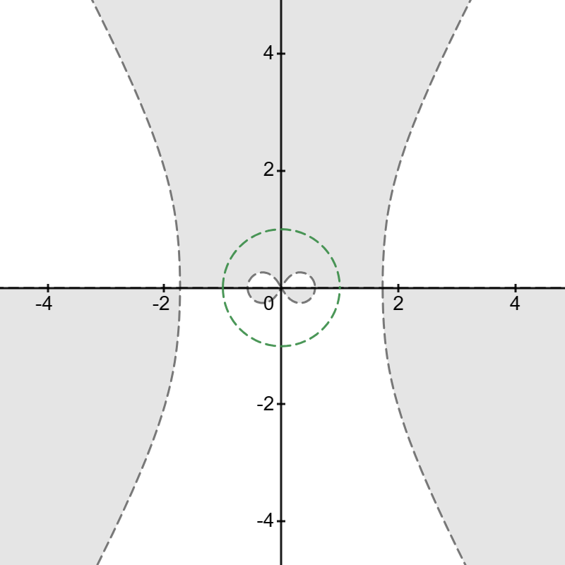
(a) $\xi<-1.5$

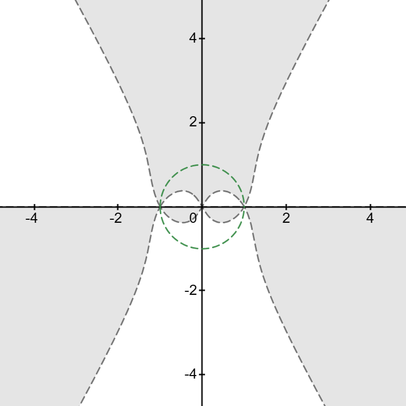
(b) $\xi=-1.5$

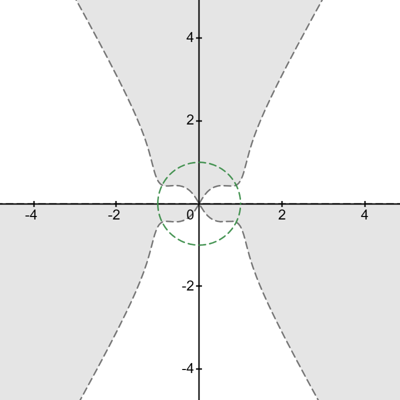
(c) $-1.5<\xi<-0.75$

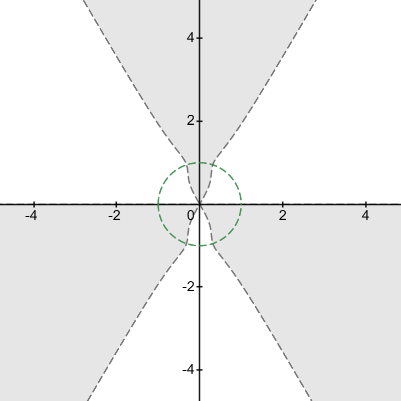
(d) $-0.75<\xi<-0.5$

(e) $\xi=-0.5$

(f) $\xi>-0.5$

Figure 3: The signature table of $\operatorname*{Re}(2i\theta(z))$. The gray dashed lines denote the critical line $\mathcal{Y}:\operatorname*{Re}(2i\theta(z))=0$. In the gray regions, we have $\operatorname*{Re}(2i\theta(z))>0$, which implies that $\left|e^{-2it\theta(z)}\right|\to 0$ as $t\to\infty$. In the white regions, $\operatorname*{Re}(2i\theta(z))<0$, which implies that $\left|e^{2it\theta(z)}\right|\to 0$ as $t\to\infty$. The green dashed circle is the unit circle $\mathcal{G}:$ $\{z\in\mathbb{C}\mid|z|=1\}$.

It is necessary to find out the stationary phase points, $\theta(z)$ differentiate respect to $z$

$$0=\theta^{\prime}(z)=\frac{1}{4z^{4}}(1+z^{2})(3+3z^{4}+4z^{2}\xi).$$ (3.12)

Form (3.12), we directly derive two fixed pure imaginary saddled points $z=\pm i$ and the distribution of the other stationary phase points based on

$$\Delta:=4\xi^{2}-9.$$

• For $\Delta>0\Longrightarrow|\xi|>\frac{3}{2}$,

  $\uuline{\xi<-\frac{3}{2}}$,    $\theta^{\prime}(z)=0$ with four different zeros on the real axis $z_{j}\in\mathbb{R},(j=1,2,3,4)$, see Figure 3(a),

  $$z_{1}=-z_{4}=\frac{\sqrt{-2\xi+\sqrt{\Delta}}}{\sqrt{3}},\ \ \ \ \ z_{2}=-z_{3}=\frac{\sqrt{-2\xi-\sqrt{\Delta}}}{\sqrt{3}}.$$ (3.13)

  We notice that $z_{4}<-1<z_{3}<0<z_{2}<1<z_{1}$ and $z_{1}z_{2}=z_{3}z_{4}=1$.

  $\uuline{\xi>-\frac{3}{2}}$,    $\theta^{\prime}(z)=0$ still with four different zeros but locate on the imaginary axis $z_{j}\in i\mathbb{R},(j=1,2,3,4)$, see Figure 3(f),

  $$z_{1}=-z_{4}=\frac{i\sqrt{2\xi+\sqrt{\Delta}}}{\sqrt{3}},\ \ \ \ \ z_{2}=-z_{3}=\frac{i\sqrt{2\xi-\sqrt{\Delta}}}{\sqrt{3}}.$$ (3.14)

  Similarly, $\operatorname*{Im}{z}_{4}<-1<\operatorname*{Im}{z}_{3}<0<\operatorname*{Im}{z}_{2}<1<\operatorname*{Im}{z}_{1}$ and $z_{1}z_{2}=z_{3}z_{4}=-1$.

• For $\Delta<0\Longrightarrow|\xi|<\frac{3}{2}$, we derive four stationary phase points on the complex plane $z_{j}\in\mathbb{C}\backslash\{\mathbb{R}\cup i\mathbb{R}\},(j=1,2,3,4)$ and $|z_{j}|=1$ which implies that the zero points controlled on the unit circle, see Figure 3(c)-3(d).

We classify the $x$-$t$ half-plane as three asymptotic regions based upon the interaction between the critical line $\mathcal{Y}$ and the unit circle $\mathcal{G}$, see Figure 1.

• solitonless region $\mathcal{D}_{1}$  and  $\mathcal{D}_{3}$: There is no interaction between the critical line $\mathcal{Y}$ and the unit circle $\mathcal{G}$ as $\xi<-3/2$ and $\xi>-1/2$. Moreover, $\mathcal{Y}$ always far away from $\mathcal{G}$, correspond with Figure 3(a) and 3(f), respectively.

• soliton region $\mathcal{D}_{2}$: For $-3/2<\xi\leq-1/2$, there are always interaction between $\mathcal{Y}$ and $\mathcal{G}$, the interaction points are hold on the unit circle $\mathcal{G}$, see Figure 3(c) and 3(d). Specially, for $\xi=-1/2$, the interaction points $z=\pm i$ locate on the imaginary axis $i\mathbb{R}$.

• $\mathbf{transition~{}region~{}\mathcal{D}_{4}}$: For $\xi=-3/2$, the interaction points between $\mathcal{Y}$ and $\mathcal{G}$ are $z=1$ and $z=-1$ which are merge points of saddle points $z_{j},j=1,2$ and $z_{j},j=3,4$, respectively, see Figure 3(b). Moreover, the norm of $(1-|r(\pm 1)|^{2})^{-1}$ blows up which implies the emergence of a new phenomenon as $\xi\approx-3/2$. The original method to deal with the cases $\xi<-\frac{3}{2}$ and $-\frac{3}{2}<\xi<\frac{3}{2}$ are broken. This case is a transition region, which is the main study region in this paper.

4 Painlevé-type asymptotics

In this section, we study the Painlevé asymptotics in the transition region $\mathcal{D}$ (1.5). In this case, the four stationary points $z_{j},j=1,2,3,4$ defined by (3.13) are real and close to $z=\pm 1$ at least the speed of $t^{-1/3}$ as $t\to\infty$.

4.1 Modifications to the basic RH problem

To get a standard RH problem without poles and singularities, we perform some modifications to the basic RH problem 3.1 by removing the poles $\nu_{n},\overline{\nu}_{n}$ and the singularities as $z=0$. Since the discrete spectrum numbers are finite and distribute on the unit circle $\mathcal{G}$. Specially, the discrete spectrum far way from the jump contour $\mathbb{R}$ and critical line $\mathcal{Y}$. The influence of the discrete spectrums are exponentially decay to identity matrix $I$ when we change their residues into jumps on some small closed circles. This permit us to modify the basic RH problem 3.1 is possible. We firstly remove the influence of discrete spectrums.

We split the set $\mathcal{N}$ into two subsets

$$\mathcal{N}_{1}:=\{n\in\mathcal{N}\mid\operatorname*{Re}(2i\theta(\nu_{n}))>0\},\ \ \mathcal{N}_{2}:=\{n\in\mathcal{N}\mid\operatorname*{Re}(2i\theta(\nu_{n}))<0\}.$$

The zero $\nu_{n}$ lead to $\left|e^{2it\theta(\nu_{n})}\right|\nrightarrow 0$ as $n\in\mathcal{N}_{1}$. For $n\in\mathcal{N}_{2}$, the zero $\nu_{n}$ lead to $\left|e^{2it\theta(\nu_{n})}\right|\rightarrow 0$. Particularly, in region $\mathcal{D}$, all $\{n\in\mathcal{N}\mid n=1,\cdots,N\}\in\mathcal{N}_{1}$, i.e. $\mathcal{N}_{1}=\mathcal{N}$ which implies that $\mathcal{N}_{2}=\varnothing$.

To remove poles $\nu_{j}$ and $\bar{\nu}_{j}$ and open the contour $\Gamma$ (which is defined in (4.2)) by a matrix decomposition in (3.11), we introduce the following function

$$T(z)=\prod_{n=1}^{N}\Bigg{(}\frac{z-\nu_{n}}{z\nu_{n}-1}\Bigg{)}\exp\left(-\frac{1}{2i\pi}\int_{\Gamma}v(\zeta)\left(\frac{1}{\zeta-z}-\frac{1}{2\zeta}\right)\,\mathrm{d}\zeta\right),$$ (4.1)

where $v(\zeta)$ is defined by (2.31) and

$$\Gamma=(-\infty,z_{4})\cup(z_{3},0)\cup(0,z_{2})\cup(z_{1},+\infty).$$ (4.2)

The properties of $T(z)$ has shown in the Proposition 4.1.

Proposition 4.1.

The function $T(z)$ is meromorphic in $\mathbb{C}\backslash\Gamma$ with simple zeros at the points $\nu_{n}$ and simple poles at the points $\bar{\nu}_{n}$, and satisfies the jump condition:

$$T_{+}(z)=T_{-}(z)(1-|r(z)|^{2}),\quad z\in\Gamma.$$

Moreover, $T(z)$ admits the following properties:

• $T(z)$ satisfies the symmetries $\overline{T(\bar{z})}=T^{-1}(z)=T(z^{-1})$.

• $T(z)$ admits the asymptotic behavior

  $$T(\infty):=\lim_{z\to\infty}T(z)=\Bigg{(}\prod_{n=1}^{N}\bar{\nu}_{n}\Bigg{)}\exp\left(\frac{1}{4i\pi}\int_{\Gamma}\frac{v(\zeta)}{\zeta}\,\mathrm{d}\zeta\right),\ \ \ \ z\to\infty.$$ (4.3)

  Moreover, $|T(\infty)|^{2}=1$. And $T(z)$ hold a asymptotic expansion

  $$T(z)=T(\infty)\Big{[}1-iz^{-1}T_{1}+\mathcal{O}(z^{-2})\Big{]},$$ (4.4)

  where

  $$T_{1}:=2\operatorname*{\sum}\limits_{n=1}^{N}{\rm Im}\nu_{n}+\frac{1}{2\pi}\int_{\Gamma}v(\zeta)d\zeta.$$

Our main goal is to construct some small regions which can remove the influence come from the discrete spectrums. To this end, we define $\rho$ which is small enough

$$0<\rho<\frac{1}{2}{\rm min}\left\{\operatorname*{min}\limits_{\nu_{n},\nu_{l}\in\mathcal{Z}^{+}}|\nu_{n}-\nu_{l}|,\operatorname*{min}\limits_{\nu_{n}\in\mathcal{Z}^{+}}|{\rm Im}\nu_{n}|,\operatorname*{min}\limits_{\nu_{n}\in\mathcal{Z}^{+},{\rm Im}\theta(z)=0}|\nu_{n}-z|\right\}.$$ (4.5)

We construct $N$ small open disks $\odot_{n}:=\{z\in\mathbb{C}^{+}\mid|z-\nu_{n}|<\rho\}$ with counter-clockwise direction on the upper-half plane. The construction way of $\odot_{n}$ ensure circles are pairwise disjoint. By the same way, $N$ open disks $\overline{\odot}_{n}:=\{z\in\mathbb{C}^{-}\mid|z-\overline{\nu}_{n}|<\rho\}$ with clockwise direction on the lower-half plane are also. We define a region $\mathcal{K}$ by

$$\mathcal{K}:=\bigcup\limits_{n=1}^{N}(\odot_{n}\cup\overline{\odot}_{n}),\ \ \partial\mathcal{K}:=\bigcup\limits_{n=1}^{N}(\partial\odot_{n}\cup\partial\overline{\odot}_{n}),$$

where $\partial\odot_{n}$ and $\partial\overline{\odot}_{n}$ denote the boundary of the disks $\odot_{n}$ and $\overline{\odot}_{n}$, respectively. The direction of real axis $\mathbb{R}$ goes from left to right, the direction of $\partial\odot_{n}$ is counterclockwise and the direction of $\partial\overline{\odot}_{n}$ is clockwise, see Figure 4. To change the residue of the pole $\nu_{n}$ into a jump on a circle $\odot_{n}$ , we define the interpolation function

$$G(z)=\begin{cases}\left(\begin{array}[]{cc}1&-\displaystyle{\frac{z-\nu_{n}}{c_{n}e^{2it\theta(\nu_{n})}}}\\ 0&1\end{array}\right),\;z\in\odot_{n},\\[4.0pt] \left(\begin{array}[]{cc}1&0\\ -\displaystyle{\frac{z-\bar{\nu}_{n}}{\bar{c}_{n}e^{-2it\theta(\bar{\nu}_{n})}}}&1\end{array}\right),\;z\in\overline{\odot}_{n},\\ I,\;\;\;else.\end{cases}$$

Define a directed contour

$$\Sigma^{(1)}=\mathbb{R}\cup\partial\mathcal{K}.$$

Figure 4: The jump contour $\Sigma^{(1)}$ of $M^{(1)}(z)$.

Make the following transformation

$$M^{(1)}(z)=T(\infty)^{-\sigma_{3}}M(z)G(z)T(z)^{\sigma_{3}},$$ (4.6)

and $M^{(1)}(z)$ satisfies the RH problem as follows.

RH problem 4.1.

Find $M^{(1)}(z)=M^{(1)}(z;x,t)$ with properties

• $M^{(1)}(z)$ is analytical in $\mathbb{C}\setminus\Sigma^{(1)}$.

• $M^{(1)}(z)=\sigma_{1}\overline{M^{(1)}(\bar{z})}\sigma_{1}=z^{-1}M^{(1)}(z^{-1})\sigma_{2}$.

• $M^{(1)}(z)$ satisfies the jump condition

  $$M^{(1)}_{+}(z)=M^{(1)}_{-}(z)V^{(1)}(z),$$

  where

  $$V^{(1)}(z)=\begin{cases}\begin{array}[]{ll}b_{-}^{-1}b_{+},\ \ \ \;z\in\Gamma,\\[8.0pt] T(z)^{-\sigma_{3}}V(z)T(z)^{\sigma_{3}},\ \ \ \;z\in\mathbb{R}\backslash\Gamma,\\[6.0pt] \left(\begin{array}[]{cc}1&-\frac{z-\nu_{n}}{c_{n}}T^{-2}(z)e^{-2it\theta(\nu_{n})}\\ 0&1\end{array}\right),\ \ \ \ z\in\partial\odot_{n},\\[12.0pt] \left(\begin{array}[]{cc}1&0\\ \frac{z-\bar{\nu}_{n}}{\bar{c}_{n}}T^{2}(z)e^{2it\theta(\bar{\nu}_{n})}&1\end{array}\right),\ \ \ \ z\in\partial\overline{\odot}_{n},\end{array}\end{cases}$$ (4.7)

  with

  $$b_{-}^{-1}b_{+}:=\left(\begin{array}[]{cc}1&-\overline{r(z)}T^{-2}(z)e^{-2it\theta(z)}\\ 0&1\end{array}\right)\left(\begin{array}[]{cc}1&0\\ r(z)T^{2}(z)e^{2it\theta(z)}&1\end{array}\right).\\$$ (4.8)

• $M^{(1)}(z)$ admits the asymptotic behaviors

  $$M^{(1)}(z)=I+\mathcal{O}(z^{-1}),\quad z\to\infty,$$

  $$M^{(1)}(z)=\frac{\sigma_{2}}{z}+\mathcal{O}(1),\quad z\to 0.$$

Remark 4.2.

The jump on $\mathbb{R}\backslash\Gamma$ without opened via the decomposition of the jump matrix $V(z)$. The aim is to match the RH problem with the Painlevé-II model in Appendix A.

Since the jump matrixes on the contour $\partial\mathcal{K}$ exponentially decay to the identity matrix as $t\to\infty$, it can be shown that the RH problem 4.1 is asymptotically equivalent to the following RH problem 4.2.

RH problem 4.2.

Find $M^{(2)}(z)=M^{(2)}(z;x,t)$ with properties

• $M^{(2)}(z)$ is analytical in $\mathbb{C}\backslash\mathbb{R}$.

• $M^{(2)}(z)=\sigma_{1}\overline{M^{(2)}(\bar{z})}\sigma_{1}=z^{-1}M^{(2)}(z^{-1})\sigma_{2}$.

• $M^{(2)}(z)$ satisfies the jump condition

  $$M^{(2)}_{+}(z)=M^{(2)}_{-}(z)V^{(2)}(z),$$ (4.9)

  where

  $$V^{(2)}(z)=\begin{cases}b_{-}^{-1}b_{+},\;z\in\Gamma,\\[6.0pt] T(z)^{-\sigma_{3}}V(z)T(z)^{\sigma_{3}},\;z\in\mathbb{R}\setminus\Gamma.\end{cases}$$ (4.10)

• $M^{(2)}(z)$ admits the asymptotic behaviors

  $$M^{(2)}(z)=I+\mathcal{O}(z^{-1}),\quad z\to\infty,$$ (4.11)

  $$M^{(2)}(z)=\frac{\sigma_{2}}{z}+\mathcal{O}(1),\quad z\to 0.$$ (4.12)

For the reason that $z=0$ is a singularity point, we removing $z=0$ by the following transformation

$$M^{(2)}(z)=J(z)M^{(3)}(z),$$ (4.13)

where

$$J(z):=I+\frac{1}{z}\sigma_{2}M^{(3)}(0)^{-1},$$ (4.14)

and $M^{(3)}(z)$ satisfies the RH problem without spectrum singularity.

RH problem 4.3.

Find $M^{(3)}(z)=M^{(3)}(z;x,t)$ with properties

• $M^{(3)}(z)$ is analytical in $\mathbb{C}\backslash\mathbb{R}$.

• $M^{(3)}(z)=\sigma_{1}\overline{M^{(3)}(\bar{z})}\sigma_{1}=\sigma_{2}M^{(3)}(0)^{-1}M^{(3)}(z^{-1})\sigma_{2}$.

• $M^{(3)}(z)$ satisfies the jump condition:

  $$M^{(3)}_{+}(z)=M^{(3)}_{-}(z)V^{(2)}(z),$$

  where $V^{(2)}(z)$ is given by (4.10).

• $M^{(3)}(z)$ admits the asymptotics $M^{(3)}(z)=I+\mathcal{O}(z^{-1}),\quad z\to\infty.$

Proof.

With the help that $M^{(2)}(z)$ satisfies the RH problem 4.2, we verify $M^{(3)}(z)$ satisfies the jump condition

$$M^{(3)}_{+}(z) =J^{-1}(z)M^{(2)}_{+}(z)=J^{-1}(z)M^{(2)}_{-}(z)V^{(2)}(z)=J^{-1}(z)J(z)M^{(3)}_{-}(z)V^{(2)}(z)=M^{(3)}_{-}(z)V^{(2)}(z).$$

To show $M^{(3)}(z)$ no singularity as $z=0$, we verify that $M^{(3)}(z)$ with the expansion

$$M^{(3)}(z)=M^{(3)}(0)+z\widetilde{M}^{(3)}(z),$$

which test and verify $M^{(2)}(z)$ satisfies (4.12). Substituting the expansion of $M^{(3)}(z)$ into (4.13) yields

$$M^{(2)}(z)=\frac{1}{z}\sigma_{2}+M^{(3)}(0)+z\widetilde{M}^{(3)}(z)+\sigma_{2}M^{(3)}(0)^{-1}\widetilde{M}^{(3)}(z)=\frac{1}{z}\sigma_{2}+\mathcal{O}(1),$$

which implies that $M^{(3)}(z)$ no singularity as $z=0$. ∎

4.2 A hybrid $\bar{\partial}$-RH problem

In this subsection, we deform the contour $\Gamma$ as shown in Figure 5 by opening the $\bar{\partial}$-lenses. This contour deformation permits us perform the $\bar{\partial}$ continuous extensions. The directed rays $\Sigma_{j}\in\mathbb{C}^{+},(j=0\pm,1,2,3,4)$ and $L_{0\pm}\in\mathbb{C}^{+}$ in Figure 5 defined by

$$\Sigma_{0+}:=he^{i\varphi},\ \ L_{0+}:=\hat{h}e^{i\pi/2}+z_{2}/2,\ \ \Sigma_{2}:=he^{i(\pi-\varphi)}+z_{2},\ \ \Sigma_{1}:=\mathbb{R}^{+}e^{i\varphi}+z_{1},$$

$$\Sigma_{0-}:=he^{i(\pi-\varphi)},\ \ L_{0-}:=\hat{h}e^{i\pi/2}+z_{3}/2,\ \ \Sigma_{3}:=he^{i\varphi}+z_{3},\ \ \Sigma_{4}:=\mathbb{R}^{+}e^{i(\pi-\varphi)}+z_{4},$$

where $h\in\left(0,\frac{1}{2}z_{2}\sec\varphi\right)$ and $\hat{h}\in\left(0,\frac{1}{2}z_{2}\tan\varphi\right)$ with a sufficiently small angle $0<\varphi<\pi/4$. The directed rays $\overline{\Sigma}_{j}\in\mathbb{C}^{-}$ and $\overline{L}_{0\pm}\in\mathbb{C}^{-}$ are the conjugate rays of $\Sigma_{j}\in\mathbb{C}^{+}$ and $L_{0\pm}\in\mathbb{C}^{+}$, respectively. We define a directed ray $\Sigma$ as

$$\Sigma:=\bigcup\limits_{j=0\pm,1,2,3,4}\left(\Sigma_{j}\cup\overline{\Sigma}_{j}\right)\bigcup\limits_{j=0\pm}\left(L_{j}\cup\overline{L}_{j}\right).$$

The regions $\Omega_{j}\subset\mathbb{C}^{+}(j=0\pm,1,2,3,4)$ in Figure 5 defined by

$$\Omega_{0+}:=\left\{z\in\mathbb{C}^{+}\mid\arg{z}\in(0,\varphi),\operatorname*{Re}z\in{(0,z_{2}/2)}\right\},\ \ \Omega_{0-}:=\left\{z\in\mathbb{C}^{+}\mid-\overline{z}\in\Omega_{0+}\right\},$$

$$\Omega_{2}:=\left\{z\in\mathbb{C}^{+}\mid\arg{z}\in(\pi-\varphi,\pi),\operatorname*{Re}z\in{(z_{2}/2,z_{2})}\right\},\ \ \Omega_{3}:=\left\{z\in\mathbb{C}^{+}\mid-\overline{z}\in\Omega_{2}\right\},$$

$$\Omega_{1}:=\left\{z\in\mathbb{C}^{+}\mid\arg{z}\in(0,\varphi),\operatorname*{Re}z\in{(z_{1},+\infty)}\right\},\ \ \Omega_{4}:=\left\{z\in\mathbb{C}^{+}\mid-\overline{z}\in\Omega_{1}\right\},$$

and $\overline{\Omega}_{j}\subset\mathbb{C}^{-}$ are the conjugate regions of $\Omega_{j}$. We define a region $\Omega$ by

$$\Omega:=\bigcup\limits_{j=0\pm,1,2,3,4}\left(\Omega_{j}\cup\overline{\Omega}_{j}\right).$$

In fact, $\Sigma$ is the boundary of $\Omega$.

Remark 4.3.

The sufficiently small angle $\varphi$ need to ensure all sectors opened by this angle fall within their respective decaying regions. Moreover, there is no intersection between $\Sigma$ and $\partial\mathcal{K}$. The same is true between $\Sigma$ and critical lines $\mathcal{Y}$, see Figure 5.

Figure 5: The jump contour $\Gamma$ be opened as $\Sigma$ .

The decaying properties of the oscillating factors $e^{\pm 2it\theta}$ in $\Omega$ is shown by the estimates of $\operatorname*{Re}(2i\theta)$ which is shown in the following Proposition 4.4.

Proposition 4.4.

In the transition region $\mathcal{D}$, $\operatorname*{Re}{(2i\theta(z))}$ holding the following estimates

• For $z\in\{\Omega_{0\pm}\cup\overline{\Omega}_{0\pm}\},$

  $$\operatorname*{Re}{(2i\theta)}\leq-c_{0}(\tilde{\varphi})|\operatorname*{Im}z||\sin{\tilde{\varphi}}|,\ \ z\in\Omega_{0\pm},$$ (4.15a)

  $$\operatorname*{Re}{(2i\theta)}\geq c_{0}(\tilde{\varphi})|\operatorname*{Im}z||\sin{\tilde{\varphi}}|,\ \ z\in\overline{\Omega}_{0\pm},$$ (4.15b)

  where $\tilde{\varphi}=\arg{z}$ and $c_{0}(\tilde{\varphi})$ depend on $\tilde{\varphi}$.

• For $z\in\{\Omega_{j}\cup\overline{\Omega}_{j}\},~{}j=1,4$,

  $$\operatorname*{Re}(2i\theta)\leq\begin{cases}-2|\operatorname*{Re}z-z_{j}|^{2}|\operatorname*{Im}z|,\ \ z\in\Omega_{j}\cap\left\{|z|\leq\sqrt{2}\right\},\\ -2(\sqrt{2}-1)|\operatorname*{Im}{z}|,\ \ z\in\Omega_{j}\cap\left\{|z|>\sqrt{2}\right\},\end{cases}$$ (4.16)

  $$\operatorname*{Re}(2i\theta)\geq\begin{cases}2|\operatorname*{Re}z-z_{j}|^{2}|\operatorname*{Im}z|,\ \ z\in\overline{\Omega}_{j}\cap\left\{|z|\leq\sqrt{2}\right\},\\ 2(\sqrt{2}-1)|\operatorname*{Im}{z}|,\ \ z\in\overline{\Omega}_{j}\cap\left\{|z|>\sqrt{2}\right\}.\end{cases}$$ (4.17)

• For $z\in\{\Omega_{j}\cup\overline{\Omega}_{j}\},~{}j=2,3$,

  $$\operatorname*{Re}(2i\theta)\leq-c(z_{j})|\operatorname*{Re}z-z_{j}|^{2}|\operatorname*{Im}z|,\ \ z\in\Omega_{j},$$ (4.18)

  $$\operatorname*{Re}(2i\theta)\geq c(c_{j})|\operatorname*{Re}z-z_{j}|^{2}|\operatorname*{Im}z|,\ \ z\in\overline{\Omega}_{j},$$ (4.19)

  where $c(z_{j})$ depend on $z_{j}$.

Proof.

For $z\in\{\Omega_{0\pm}\cup\overline{\Omega}_{0\pm}\}$, we take $z\in\Omega_{0+}$ as an example and the rest regions can be derived as the same method. Let $z=|z|e^{i\tilde{\varphi}}=u+iv$ where $u>v>0$ and $0<\tilde{\varphi}<\varphi$. Define a function $F(l)=l+l^{-1}$ with $l>0$. Rewrite $\operatorname*{Re}{(2i\theta)}$ as

$$\operatorname*{Re}{(2i\theta)}=-F(|z|)\sin{\tilde{\varphi}}g(z),$$

where

$$g(z)=2\xi-3\cos{2\tilde{\varphi}}+\frac{1}{2}F^{2}(|z|)(1+2\cos{2\tilde{\varphi}}).$$

As $\operatorname*{Re}{(2i\theta)}=0$, we have

$$g(z)=2\xi-3\cos{2\tilde{\varphi}}+\frac{1}{2}F^{2}(|z|)(1+2\cos{2\tilde{\varphi}})=0.$$ (4.20)

This equation (4.20) implies that

$$4<\alpha:=F^{2}(|z|)=3-\frac{4\xi+3}{1+2\cos{2\tilde{\varphi}}}.$$

Furtherly, we have $F(|z|)=|z|+|z|^{-1}=\sqrt{\alpha}$, which admits two solutions

$$|z|_{1}=\frac{\sqrt{\alpha}-\sqrt{\alpha-4}}{2},\ \ |z|_{2}=\frac{\sqrt{\alpha}+\sqrt{\alpha-4}}{2},$$

and $|z|_{1}<|z|_{2}$. It is easy to check that $h(l):=l^{2}-\sqrt{\alpha}l+1$ is a monotonically increasing function as $l\in\left(\frac{\sqrt{\alpha}}{2},+\infty\right)$. And it is a monotonically decreasing function as $l\in\left(-\infty,\frac{\sqrt{\alpha}}{2}\right)$. Since $|z|_{1}<\frac{\sqrt{\alpha}}{2}$, $h(l)$ is monotonically decreasing on $(0,|z|_{1})$. We have $h(l)>h(|z|_{1})=0$ and $F(l)>\sqrt{\alpha}$, which implies that

$$g(z)>0.$$

There exists a constant $c_{0}=c_{0}(\tilde{\varphi})$ such that

$$\operatorname*{Re}{(2i\theta)}\leq-c_{0}F(|z|)\sin{\tilde{\varphi}}=-c_{0}\sqrt{\alpha}\sin{\tilde{\varphi}}.$$

We derive the equations (4.15).

For $z\in\{\Omega_{j}\cup\overline{\Omega}_{j}\}_{j=1}^{4}$, we proof $z\in\Omega_{1}$ and the rest regions can be proofed by the same method. Let $z=z_{1}+u+iv=z_{1}+|z-z_{1}|e^{i\tilde{\varphi}}\in\Omega_{1}$, where $u>0$ and $v=u\tan{\tilde{\varphi}}>0,|z|^{2}=(u+z_{1})^{2}+u^{2}\tan^{2}\tilde{\varphi}.$ By some simplification, $\operatorname*{Re}(2i\theta)$ can be rewritten as

$$\operatorname*{Re}(2i\theta) =-vg(u,v),$$

where

$$g(u,v) =\left(1+\frac{1}{|z|^{6}}\right)\left(3(z_{1}+u)^{2}-v^{2}+\frac{|z|^{6}+|z|^{4}}{|z|^{6}+1}\left(2\xi+\frac{3}{2}\right)\right)$$

$$>3(z_{1}+u)^{2}-v^{2}+\frac{|z|^{6}+|z|^{4}}{|z|^{6}+1}\left(2\xi+\frac{3}{2}\right)$$

$$:=f(u,v).$$

Let $h(|z|):=\frac{|z|^{6}+|z|^{4}}{|z|^{6}+1}$, and $h(|z|)$ with the max/min value

$$\begin{cases}0\leq h(|z|)\leq\frac{4}{3},\ \ |z|\leq\sqrt{2},\\ 1<h(|z|)\leq\frac{4}{3},\ \ |z|>\sqrt{2}.\end{cases}$$ (4.21)

For $|z|\leq\sqrt{2}$, from the relation (3.13), we have

$$\xi=-\frac{3z_{1}^{4}+3}{4z_{1}^{2}}\Longrightarrow 2\xi+\frac{3}{2}=-\frac{3}{2}(z_{1}^{2}+z_{1}^{-2}-1).$$ (4.22)

Substituting (4.22) into $f(u,v)$, we have

$$f(u,v)=3(z_{1}+u)^{2}-v^{2}-\frac{3}{2}h(|z|)(z_{1}^{2}+z_{1}^{-2}+1).$$

By some estimates for $f(u,v)$ under the condition (4.21), we have

$$f(u,v)\geq 3(z_{1}+u)^{2}-v^{2}-2(z_{1}^{2}+z_{1}^{-2}+1).$$

For the reason that $v=(z_{1}+u)\tan{\tilde{\varphi}}$ and $0<\tilde{\varphi}<\varphi<\frac{\pi}{4}$,

$$f(u,v) \geq 3(z_{1}+u)^{2}-(z_{1}+u)^{2}\tan^{2}{\tilde{\varphi}}-2(z_{1}^{2}+z_{1}^{-2}+1)$$

$$>2u^{2}+4z_{1}u-2(z_{1}^{-2}+1)$$

$$\geq 2u^{2}.$$

For $|z|>\sqrt{2}$, moreover, $\xi\rightarrow\left(-\frac{3}{2}\right)^{-}$,

$$f(u,v)=3(z_{1}+u)^{2}-v^{2}-\frac{3}{2}h(|z|).$$

Considering the condition (4.21) as $|z|>\sqrt{2}$, and $v=(z_{1}+u)\tan{\tilde{\varphi}}$ with $0<\tilde{\varphi}<\varphi<\frac{\pi}{4}$,

$$f(u,v) \geq 3(z_{1}+u)^{2}-v^{2}-2$$

$$\geq 2(z_{1}+u)^{2}-2$$

$$\geq 4\cos{\tilde{\varphi}}-2$$

$$\geq 2(\sqrt{2}-1).$$

The third case can derived by the same way. ∎

Next we perform continuous extensions for the jump matrix $V^{(2)}$ to remove the jump from $\Gamma$.

Lemma 4.5.

Let $q_{0}(x)\in\tanh x+L^{1,2}(\mathbb{R})$. There exist the boundary value functions $R_{j}(z):\overline{\Omega}_{j}\mapsto\mathbb{C},j=0\pm,1,2,3,4$ continuous on $\overline{\Omega}_{j}$ and with continuous first partial derivative on $\Omega_{j}$, which defined by

$$R_{j}(z)=\begin{cases}r(z)T^{2}(z),\quad z\in\Gamma,\\ r(z_{j})T^{2}(z_{j}),\ \ z\in\Sigma_{j},\ j=1,2,3,4,\\ 0,\quad z\in\Sigma_{0\pm},\ j=0\pm,\end{cases}$$

the conjugate function $\overline{R}_{j}(z)$ is given by

$$\overline{R}_{j}(z)=\begin{cases}\overline{r}(z)T^{-2}(z),\quad z\in\Gamma,\\ \overline{r}(z_{j})T^{-2}(z_{j}),\ \ z\in\overline{\Sigma}_{j},\ j=1,2,3,4,\\ 0,\quad z\in\overline{\Sigma}_{0\pm},\ j=0\pm.\end{cases}$$

There exist a constant $c:=c(q_{0})$ and a cutoff function $\omega\in C_{0}^{\infty}(\mathbb{R},[0,1])$ with small support near 1. We have

$$|\overline{\partial}R_{j}|,|\overline{\partial}\overline{R}_{j}|\leq\begin{cases}c(|r^{\prime}(|z|)|+|z-z_{j}|^{-1/2}+\varphi(|z|)),\ \ z\in\Omega_{j}\cup\overline{\Omega}_{j},\\ c|z-1|,\ \ z\in\Omega_{j}\cup\overline{\Omega}_{j}~{}and~{}|z-1|~{}small~{}enough,\\ c(|r^{\prime}(\pm|z|)|+|z|^{-1/2}),\ \ z\in\Omega_{0\pm}\cup\overline{\Omega}_{0\pm}.\end{cases}$$

Moreover, setting $R:\Omega\mapsto\mathbb{C}$ by $R(z)|_{z\in\Omega_{j}}=R_{j}(z)$ and $R(z)|_{z\in\overline{\Omega}_{j}}=\overline{R}_{j}(z)$, the extension can be made such that $R(z)=\overline{R}(\overline{z}^{-1})$.

Define a matrix function

$$R^{(3)}(z)=\begin{cases}\left(\begin{array}[]{cc}1&0\\ -R_{j}(z)e^{2it\theta(z)}&1\end{array}\right),\quad z\in\Omega_{j},\ j=0\pm,1,2,3,4,\\ \left(\begin{array}[]{cc}1&-\overline{R}_{j}(z)e^{-2it\theta(z)}\\ 0&1\end{array}\right),\quad z\in\overline{\Omega}_{j},\ j=0\pm,1,2,3,4,\\ I,\quad{else}.\end{cases}$$ (4.23)

and define a new contour

$$\Sigma^{(4)}=\bigcup\limits_{j=0\pm}(L_{j}\cup\overline{L}_{j})\cup[z_{4},z_{3}]\cup[z_{2},z_{1}].$$

We make a new transformation

$$M^{(4)}(z)=M^{(3)}(z)R^{(3)}(z),$$ (4.24)

where $M^{(4)}(z)$ satisfies the following hybrid $\bar{\partial}$-RH problem.

$\bar{\partial}$-RH problem 4.1.

Find $M^{(4)}(z)=M^{(4)}(z;x,t)$ with properties

• $M^{(4)}(z)$ is continuous in $\mathbb{C}\setminus\Sigma^{(4)}$. See Figure 6.

• $M^{(4)}(z)$ satisfies the jump condition

  $$M^{(4)}_{+}(z)=M^{(4)}_{-}(z)V^{(4)}(z),$$ (4.25)

where

$$V^{(4)}(z)=\begin{cases}\left(\begin{array}[]{cc}1&0\\ r\left(z_{j}\right)T^{2}(z_{j})e^{2it\theta(z)}&1\end{array}\right),\ z\in\Sigma_{j},\ j=1,2,3,4;\vspace{2mm}\\ \left(\begin{array}[]{cc}1&-\overline{r}\left(z_{j}\right)T^{-2}(z_{j})e^{-2it\theta(z)}\\ 0&1\end{array}\right),\ z\in\overline{\Sigma}_{j},\ j=1,2,3,4;\vspace{2mm}\\ \left(\begin{array}[]{cc}1&0\\ r\left(z_{2}\right)T^{2}(z_{2})e^{2it\theta(z)}&1\end{array}\right),\ z\in L_{0+};\vspace{2mm}\\ \left(\begin{array}[]{cc}1&-\overline{r}\left(z_{2}\right)T^{-2}(z_{2})e^{-2it\theta(z)}\\ 0&1\end{array}\right),\ z\in\overline{L}_{0+};\vspace{2mm}\\ \left(\begin{array}[]{cc}1&0\\ -r\left(z_{3}\right)T^{2}(z_{3})e^{2it\theta(z)}&1\end{array}\right),\ z\in L_{0-};\vspace{2mm}\\ \left(\begin{array}[]{cc}1&\overline{r}\left(z_{3}\right)T^{-2}(z_{3})e^{-2it\theta(z)}\\ 0&1\end{array}\right),\ z\in\overline{L}_{0-};\vspace{2mm}\\ T(z)^{-\sigma_{3}}V(z)T(z)^{\sigma_{3}},\quad z\in\mathbb{R}\backslash\Gamma.\end{cases}$$ (4.26)

• $M^{(4)}(z)$ has the asymptotic behavior: $M^{(4)}(z)=I+\mathcal{O}(z^{-1}),\quad z\to\infty.$

• For $z\in\mathbb{C}\setminus\Sigma^{(4)}$, we have

  $$\bar{\partial}M^{(4)}(z)=M^{(4)}(z)\bar{\partial}R^{(3)}(z),$$

  where

  $$\bar{\partial}R^{(3)}(z)=\begin{cases}\left(\begin{array}[]{cc}0&0\\ -\bar{\partial}R_{j}(z)e^{2it\theta(z)}&0\end{array}\right),\quad z\in\Omega_{j},\ j=0\pm,1,2,3,4,\\ \left(\begin{array}[]{cc}0&-\bar{\partial}\overline{R}_{j}(z)e^{-2it\theta(z)}\\ 0&0\end{array}\right),\quad z\in\overline{\Omega}_{j},\ j=0\pm,1,2,3,4,\\ 0,\quad{else}.\end{cases}$$ (4.27)

In the next subsection, we decompose $M^{(4)}(z)$ into a pure RH problem $M^{rhp}(z)$ with $\bar{\partial}R^{(3)}(z)=0$ and a pure $\bar{\partial}$-problem $M^{(5)}(z)$ with $\bar{\partial}R^{(3)}(z)\neq 0$ in the form

$$M^{(4)}(z)=\begin{cases}M^{rhp}(z)\Longrightarrow\bar{\partial}R^{(3)}(z)=0,\\ M^{(5)}(z)M^{rhp}(z)\Longrightarrow\bar{\partial}R^{(3)}(z)\neq 0.\end{cases}$$ (4.28)

Figure 6: The jump contour $\Sigma^{(4)}$.

4.3 Pure RH problem

In this subsection, we consider the contribution of the pure RH problem for the long-time asymptotics solution. The pure RH problem is given as follows.

RH problem 4.4.

Find $M^{rhp}(z)=M^{rhp}(z;x,t)$ which satisfies

• $M^{rhp}(z)$ is analytical in $\mathbb{C}\backslash\Sigma^{(4)}$. See Figure 6.

• $M^{rhp}(z)$ satisfies the jump condition

  $$M^{rhp}_{+}(z)=M^{rhp}_{-}(z)V^{(4)}(z),$$

  where $V^{(4)}(z)$ is given by (4.26).

• $M^{rhp}(z)$ has the same asymptotics with $M^{(4)}(z)$.

We consider the local models of $M^{rhp}(z)$ as $z=\pm 1$. For a fixed parameter $0<\varepsilon<\sqrt{2C}$, we define two open disks in the neighborhood of $z=\pm 1$,

$$\mathcal{U}_{L}:=\{z\in\mathbb{C}:|z+1|<\varepsilon\tau^{-1/3+\varsigma}\},\ \ \mathcal{U}_{R}:=\{z\in\mathbb{C}:|z-1|<\varepsilon\tau^{-1/3+\varsigma}\},$$

the boundaries $\partial\mathcal{U}_{L}$ and $\partial\mathcal{U}_{R}$ with oriented counterclockwise, see Figure 6. The parameter $\varsigma$ is a constant and controlled by $0<\varsigma<1/6$ and $\sqrt{2C}\tau^{-1/3+\varsigma}<\rho$ as $t$ is large enough, $\rho$ is defined by (4.5). The saddle points belong to the corresponding disks

$$z_{1},z_{2}\in\mathcal{U}_{R},\ \ \ \ z_{3},z_{4}\in\mathcal{U}_{L}.$$

In the disks $\mathcal{U}_{L}$ and $\mathcal{U}_{R}$, there exist two local RH problem associated with $M_{L}(z)$ and $M_{R}(z)$.

In fact, jump matrix $V^{(4)}$ decays to a identity matrix outside $\mathcal{U}_{L}$ and $\mathcal{U}_{R}$ exponentially and uniformly fast as $t\to+\infty$. This enlightens us to reconstruct the solution of $M^{rhp}(z)$ as the following three cases:

$$M^{rhp}(z)=\begin{cases}M^{err}(z),\quad z\in\mathbb{C}\setminus\{\mathcal{U}_{L}\cup\mathcal{U}_{R}\},\\ M^{err}(z)M_{L}(z),\quad z\in\mathcal{U}_{L},\\ M^{err}(z)M_{R}(z),\quad z\in\mathcal{U}_{R},\end{cases}$$ (4.29)

where $M^{err}(z)$ is an error function which will be determined in the subsection 4.3.2 via a small norm RH problem. $M_{L}(z)$ and $M_{R}(z)$ admit local models near $z=-1$ and $z=1$, which are approximated by RH problem associated to Painlevé II transcendents. We expound the local model $M_{R}(z)$ as $z=1$, the local model $M_{L}(z)$ can derived with the similar way.

The local RH problem of $M_{R}(z)$ as follows.

RH problem 4.5.

Find $M_{R}(z):=M_{R}(z,x,t)$ with properties

• $M_{R}(z)$ is analytical in $\mathcal{U}_{R}\backslash{\Sigma}_{R}$, where $\Sigma_{R}=\Sigma^{(4)}\cap\mathcal{U}_{R}$. See Figure 7.

• $M_{R}(z)$ satisfies the jump condition

  $$M_{R+}(z)=M_{R-}(z){V}_{R}(z),\ z\in{\Sigma}_{R},$$

where

$$V_{R}(z)=\begin{cases}\left(\begin{array}[]{cc}1&0\\ r(z_{j})T^{2}(z_{j})e^{2it\theta(z)}&1\end{array}\right),\ z\in\{\Sigma_{j}\cap\mathcal{U}_{R}\},\ j=1,2,\\ \left(\begin{array}[]{cc}1&-\overline{r(z_{j})}T^{-2}(z_{j})e^{-2it\theta(z)}\\ 0&1\end{array}\right),\ z\in\{\overline{\Sigma}_{j}\cap\mathcal{U}_{R}\},\ j=1,2,\\ T(z)^{-\sigma_{3}}V(z)T(z)^{\sigma_{3}},\ z\in(z_{2},z_{1}).\end{cases}$$ (4.30)

• $M_{R}(z)(I+\mathcal{O}(t^{-1/3}))^{-1}\to I,\ t\to+\infty$, uniformly for $z\in\partial\mathcal{U}_{R}.$

4.3.1 Local solvable RH problem

In the region $\mathcal{D}$, we have $\xi\to\left(-\frac{3}{2}\right)^{-}$ as $t\to+\infty$, further from (3.13)-(3.14), it is found that the phase points $z_{1}$ and $z_{2}$ will merge to $z=1$, while $z_{3}$ and $z_{4}$ will merge to $z=-1$.

We seek a polynomial fitting for the phase function $t\theta(z)$ as $z=1$, we find that

$$t\theta(z)={} 3t(z-1)^{3}+(x+3t)(z-1)+\frac{1}{2}x\left(\sum_{n=2}^{\infty}(-1)^{n-1}(z-1)^{n}\right)$$

$$+\frac{1}{4}t\left(3(z-1)^{2}-11(z-1)^{3}+\sum_{n=2}^{\infty}(-1)^{n-1}\frac{n^{2}+3n+8}{2}(z-1)^{n}\right)$$

$$\xlongequal{z\mapsto\hat{k}}{} \frac{4}{3}\hat{k}^{3}+s\hat{k}+\mathcal{O}(t^{-1/3}\hat{k}^{2}),$$ (4.31)

where

$$\hat{k}=\tau^{\frac{1}{3}}(z-1),\ \ s=\frac{8}{9}\left(\xi+\frac{3}{2}\right)\tau^{\frac{2}{3}},\ \ \tau=\frac{9}{4}t.$$ (4.32)

In the same way, we notice that the phase function $t\theta(z)$ with the same property as $z=-1$. It is shown as follow

$$t\theta(z)={} 3t(z+1)^{3}+(x+3t)(z+1)+\frac{1}{2}x\left(\sum_{n=2}^{\infty}(z+1)^{n}\right)$$

$$+\frac{1}{4}t\left(-3(z+1)^{2}-11(z+1)^{3}+\sum_{n=2}^{\infty}\frac{n^{2}+3n+8}{2}(z+1)^{n}\right)$$

$$\xlongequal{z\mapsto\check{k}}{} \frac{4}{3}\check{k}^{3}+s\check{k}+\mathcal{O}(t^{-1/3}\check{k}^{2}),$$ (4.33)

where $s,\tau$ are defined by (4.32), and

$$\check{k}=\tau^{\frac{1}{3}}(z+1).$$ (4.34)

The scaling transformation (4.32) and (4.34) permit us close to the Painlevé-II RH model. In addition, the new phase points $\hat{k}_{j}$ and $\check{k}_{j}$ with the properties:

Proposition 4.6.

In the transition region $\mathcal{D}$ (1.5), the scaling transformations (4.32) and (4.34) lead to four new phase points $\hat{k}_{j}=\tau^{1/3}(z_{j}-1),\ j=1,2$ and $\check{k}_{j}=\tau^{1/3}(z_{j}+1),\ j=3,4$ which always hold by a constant

$$\left|\hat{k}_{1}\right|<2(9/4)^{1/3}\sqrt{2C},\ \ \left|\hat{k}_{2}\right|<(9/4)^{1/3}\sqrt{2C},$$

$$\left|\check{k}_{3}\right|<(9/4)^{1/3}\sqrt{2C},\ \ \left|\check{k}_{4}\right|<2(9/4)^{1/3}\sqrt{2C}.$$

Proof.

From (3.12), we have the phase points $z_{j},j=1,2$ satisfies the equation

$$3(\chi^{2}_{j}-2)+4\xi=0,$$

where $\chi_{j}=z_{j}+z_{j}^{-1}$ and $\chi_{j}$ admits the relation

$$\chi_{j}=-\frac{4}{3}\xi+2.$$

For the reason that $z_{1},z_{2}\to 1$ as $t\to\infty$, we take a large $t$ such that $\frac{1}{2}<z_{2}<1$. Furtherly, we have

$$z_{2}^{2}+1=\chi_{2}z_{2}\Longrightarrow(z_{2}-1)^{2}=(\chi_{2}-2)z_{2}.$$ (4.35)

Noting that $\chi_{2}-2>0$ and $0<z_{2}<1$, we have

$$(\chi_{2}-2)z_{2}<\chi_{2}-2=-\frac{4}{3}\xi<-2\left(\xi+\frac{3}{2}\right).$$ (4.36)

Substituting (4.36) into (4.35) yields

$$(z_{2}-1)^{2}<-2\left(\xi+\frac{3}{2}\right)<2Ct^{-2/3},$$ (4.37)

which implies that

$$\big{|}\hat{k}_{2}\big{|}=\big{|}\tau^{1/3}(z_{2}-1)\big{|}<(9/4)^{1/3}\sqrt{2C}.$$ (4.38)

Recalling that the symmetry $z_{1}z_{2}=1$ which implies that $z_{1}>1$. We have

$$z_{1}-1=\frac{1}{z_{2}}-1=\frac{1-z_{2}}{z_{2}}.$$

With the help of (4.38), we derive $\hat{k}_{1}$ can be controlled by a constant

$$\big{|}\hat{k}_{1}\big{|}=\big{|}\tau^{1/3}(z_{1}-1)\big{|}=\left|\frac{\tau^{1/3}(1-z_{2})}{z_{2}}\right|<2(9/4)^{1/3}\sqrt{2C}.$$

From (3.13), we have $z_{3}=-z_{2}$ and $z_{4}=-z_{1}$, the estimate of $\left|\check{k}_{j}\right|$ can be derived. ∎

We define two open disks in the neighborhood of $\hat{k}=0$ and $\check{k}=0$, respectively,

$$\check{\mathcal{U}}_{L}:=\{\check{k}\in\mathbb{C}:|\check{k}|<\varepsilon\tau^{\varsigma}\},\ \ \hat{\mathcal{U}}_{R}:=\{\hat{k}\in\mathbb{C}:|\hat{k}|<\varepsilon\tau^{\varsigma}\},$$

which with oriented counterclockwise. There are new saddle points $\hat{k}_{j},j=1,2$ and $\check{k}_{j},j=3,4$ under the maps $z\mapsto\hat{k}$ (4.31) and $z\mapsto\check{k}$ (4.33), respectively, which belong to the corresponding disks

$$\hat{k}_{1},\hat{k}_{2}\in\hat{\mathcal{U}}_{R},\ \ \ \ \check{k}_{3},\check{k}_{4}\in\check{\mathcal{U}}_{L}.$$

The transformation (4.32) and (4.34) map $\mathcal{U}_{R}$ into $\hat{\mathcal{U}}_{R}$ and map $\mathcal{U}_{L}$ into $\check{\mathcal{U}}_{L}$, respectively, see Figure 6.

Figure 7: The jump contours of $\Sigma_{R}$ (left) and $\hat{\Sigma}_{R}$ (right).

Next we show that the local RH problem $M_{R}(z)$ can be approximated by the solution of a model RH problem for Painlevé-II equation. From (4.32), we have

$$z=\tau^{-1/3}\hat{k}+1,$$

and let $\widetilde{r}(z):=r(z)T^{2}(z)=r(\tau^{-1/3}\hat{k}+1)T^{2}(\tau^{-1/3}\hat{k}+1).$ Particularly, we have $\widetilde{r}(1)=r(1)T^{2}(1)$ and derive the following estimates of $\operatorname*{Re}\left(2i\left(\frac{4}{3}\hat{k}^{3}+s\hat{k}\right)\right)$.

Lemma 4.7.

For $t\rightarrow\infty$, we have the following estimates

$$\operatorname*{Re}\left(2i\left(\frac{4}{3}\hat{k}^{3}+s\hat{k}\right)\right)\leq-4\hat{u}^{2}\hat{v},\ \ \hat{k}\in\hat{\Omega}_{j},\ \ j=1,2,$$ (4.39)

$$\operatorname*{Re}\left(2i\left(\frac{4}{3}\hat{k}^{3}+s\hat{k}\right)\right)\geq 4\hat{u}^{2}\hat{v},\ \ \hat{k}\in\overline{\hat{\Omega}}_{j},\ \ j=1,2,$$ (4.40)

where $\hat{k}=\hat{k}_{1}+\hat{u}+i\hat{v}$.

Proof.

Let $z=z_{1}+u+iv$. For the reason that $\arg(z-z_{1})<\pi/4$, we have $v<u$.

$$\operatorname*{Re}\left(2i\left(\frac{4}{3}\hat{k}^{3}+s\hat{k}\right)\right) =\operatorname*{Re}\left(2i\left(3t(z-1)^{3}+2(x+3t)(z-1)\right)\right)$$

$$\leq-12tu^{2}v+3tv\omega(z_{1}),$$

where

$$\omega(z_{1})=-\left(\left((-1+z_{1})\left(1+z_{1}+5z_{1}^{3}+z_{1}^{2}(-7+12u)\right)\right)/z_{1}^{2}\right),$$

and $\omega^{\prime}(z_{1})\leq 0$. We derive $\omega(z_{1})\leq\omega(1)=0$. We derive (4.39). The next (4.40) can be derived by the same estimate. ∎

Proposition 4.8.

For $j=1,2$, we have the following estimates

$$\Big{|}\widetilde{r}\left(z\right)e^{2it\theta\left(z\right)}-r_{0}e^{8i\hat{k}^{3}/3+2is\hat{k}}\Big{|}\lesssim t^{-1/3+2\varsigma},\ \hat{k}\in\left(\hat{k}_{2},\hat{k}_{1}\right),$$ (4.41)

$$\Big{|}\widetilde{r}\left(z_{j}\right)e^{2it\theta\left(z\right)}-r_{0}e^{8i\hat{k}^{3}/3+2is\hat{k}}\Big{|}\lesssim t^{-1/3+2\varsigma},\ \hat{k}\in\hat{\Sigma}_{R}\setminus[\hat{k}_{2},\hat{k}_{1}],$$ (4.42)

where $r_{0}=\widetilde{r}(1)$.

Proof.

For $\hat{k}\in\left(\hat{k}_{2},\hat{k}_{1}\right)$, $\hat{k}$ is real and $z\in(z_{2},z_{1})$.

$$\left|\widetilde{r}(z)e^{2it\theta\left(z\right)}-r_{0}e^{8i\hat{k}^{3}/3+2is\hat{k}}\right|\leq\left|\widetilde{r}(z)-\widetilde{r}(1)\right|+\left|\widetilde{r}(1)\right|\left|e^{2it\theta\left(z\right)}-e^{8i\hat{k}^{3}/3+2is\hat{k}}\right|.$$ (4.43)

For the reason that $T(z)$ is analytic in $\partial\mathcal{U}_{R}$, we have

$$\parallel\widetilde{r}(z)\parallel_{H^{1}([z_{2},z_{1}])}=\parallel r(z)\parallel_{H^{1}([z_{2},z_{1}])},$$

and with the help of the Hölder inequality, we derive the following estimate

$$\left|\widetilde{r}(z)-\widetilde{r}(1)\right|=\left|\int_{1}^{z}\widetilde{r}^{\prime}(s)\mathrm{d}s\right| \leq\parallel\widetilde{r}^{\prime}\parallel_{L^{2}([z_{2},z_{1}])}\left|z-1\right|^{1/2}t^{-1/6}$$

$$\leq\parallel r\parallel_{H^{1}([z_{2},z_{1}])}\left|\hat{k}\right|^{1/2}t^{-1/3+\varsigma/2}$$

$$\lesssim t^{-1/3+\varsigma/2}.$$

In addition,

$$\left|e^{2it\theta\left(z\right)}-e^{8i\hat{k}^{3}/3+2is\hat{k}}\right|=\left|e^{i\mathcal{O}(t^{-1/3}\hat{k}^{2})}-1\right|\leq e^{|\mathcal{O}(t^{-1/3}\hat{k}^{2})|}-1\lesssim t^{-1/3+2\varsigma}.$$

From Lemma 4.7, we have $\left|e^{2i\left(\frac{4}{3}\hat{k}^{3}+s\hat{k}\right)}\right|$ is bounded. As in the above proof, we can obtain the estimate (4.42). The estimate on the other jump line can be given similarly. ∎

Now, we find a new RH problem associated with $\hat{M}_{R}(\hat{k})$ in the disk $\hat{\mathcal{U}}_{R}$:

RH problem 4.6.

Find $\hat{M}_{R}(\hat{k})=\hat{M}_{R}(\hat{k},x,t)$ with properties

• $\hat{M}_{R}(\hat{k})$ is analytical in $\hat{\mathcal{U}}_{R}\backslash\hat{\Sigma}_{R}$, where $\hat{\Sigma}_{R}=\hat{\Sigma}_{j}\cap\hat{\mathcal{U}}_{R}$, see Figure 7.

• $\hat{M}_{R}(\hat{k})$ satisfies the jump condition

  $$\hat{M}_{R+}(\hat{k})=\hat{M}_{R-}(\hat{k})\hat{V}_{R}(\hat{k}),\ z\in\hat{\Sigma}_{R},$$

where

$$\hat{V}_{R}(\hat{k})=\begin{cases}\left(\begin{array}[]{cc}1&0\\ \tilde{r}(1)e^{2i\left(\frac{4}{3}\hat{k}^{3}+s\hat{k}\right)}&1\end{array}\right):=B_{+},\ \hat{k}\in\hat{\Sigma}_{j},\ j=1,2;\\ \left(\begin{array}[]{cc}1&-\overline{\tilde{r}(1)}e^{-2i\left(\frac{4}{3}\hat{k}^{3}+s\hat{k}\right)}\\ 0&1\end{array}\right):=B_{-}^{-1},\ \hat{k}\in\overline{\hat{\Sigma}}_{j},\ j=1,2;\\ B_{-}^{-1}B_{+},\ \hat{k}\in(\hat{k}_{2},\hat{k}_{1}).\end{cases}$$ (4.44)

• $\hat{M}_{R}(\hat{k})\to I$, as $\hat{k}\to+\infty.$

Define $\Lambda(\hat{k}):=M_{R}(\hat{k})\hat{M}_{R}^{-1}(\hat{k})$. The estimate in Proposition 4.8 implies that $\Lambda(\hat{k})$ admits the following asymptotic behavior.

Lemma 4.9.

In the disk $\hat{\mathcal{U}}_{R}$, $\Lambda(\hat{k})$ admits the asymptotic behavior for a large $t$

$$\Lambda(\hat{k})=I+\mathcal{O}(t^{-1/3+2\varsigma}),\ \ t\to+\infty.$$ (4.45)

Moreover, $\Lambda(\hat{k})$ satisfies a RH problem:

RH problem 4.7.

Find $\Lambda(\hat{k}):=\Lambda(\hat{k},x,t)$ with properties:

• $\Lambda(\hat{k})$ is analytical in $\mathbb{C}\backslash\hat{\Sigma}_{R}$.

• $\Lambda(\hat{k})$ satisfies the following jump condition

  $$\Lambda_{+}(\hat{k})=\Lambda_{-}(\hat{k})V_{\Lambda}(\hat{k}),$$

  where

  $$V_{\Lambda}(\hat{k})=\hat{M}_{R,-}(\hat{k})V_{R}(\hat{k})\hat{V}^{-1}_{R}(\hat{k})\hat{M}^{-1}_{R,-}(\hat{k}).$$ (4.46)

We derive the following Corollary 4.10 from (4.45) and (4.46).

Corollary 4.10.

In the transition region $\mathcal{D}$ (1.5), as $t\to\infty$, we have

$$V_{R}\left(z\right)=\hat{V}_{R}(\hat{k})+\mathcal{O}(t^{-1/3+2\varsigma}),\ \ \hat{k}\in\hat{\mathcal{U}}_{R},$$

$$M_{R}\left(z\right)=\hat{M}_{R}(\hat{k})+\mathcal{O}(t^{-1/3+2\varsigma}),\ \ \hat{k}\in\hat{\mathcal{U}}_{R},$$

For associated with Painlevé-II RH model, we add four auxiliary contours $\mathcal{L}_{j},~{}j=1,2,3,4$ which are passing through the point $\hat{k}=0$. And the angle of $\mathcal{L}_{j}$ with real axis is $\pi/3$. $\mathcal{L}_{j}$ together with the original contours $\hat{\Sigma}_{j}$ divide the complex plane $\mathbb{C}$ into eight regions $\Omega^{\flat}_{j},~{}j=1,\cdots,8$, see Figure 8.

Figure 8: In the left figure, we add four auxiliary contours on the jump contour for $\hat{M}_{R}(\hat{k})$, which can be deformed into the Painlevé-II model $M_{P}(\hat{k})$ with the jump contour of four rays (the right one).

We define a matrix valued function

$$P(\hat{k})=\begin{cases}B_{+}^{-1},\quad\hat{k}\in\Omega^{\flat}_{2}\cup\Omega^{\flat}_{4},\\ B_{-}^{-1},\quad\hat{k}\in\Omega^{\flat}_{6}\cup\Omega^{\flat}_{8},\\ I,\quad else,\end{cases}$$

and $\hat{M}_{R}(\hat{k})$ performing the following transformation

$$\mathcal{M}_{R}(\hat{k})=\hat{M}_{R}(\hat{k})P(\hat{k}).$$

$\mathcal{M}_{R}(\hat{k})$ admits the following RH problem.

RH problem 4.8.

Find $\mathcal{M}_{R}(\hat{k})=\mathcal{M}_{R}(\hat{k},s)$ with properties

• $\mathcal{M}_{R}(\hat{k})$ is analytical in $\mathbb{C}\backslash\Sigma_{P}$, where $\Sigma_{P}=\bigcup\limits_{j=1}^{4}\mathcal{L}_{j}$.

• $\mathcal{M}_{R}(\hat{k})$ satisfies the jump condition

  $$\mathcal{M}_{R,+}(\hat{k})=\mathcal{M}_{R,-}(\hat{k})\mathcal{V}_{R}(\hat{k}),\ \hat{k}\in\Sigma_{P},$$

  where

  $$\mathcal{V}_{P}(\hat{k})=\begin{cases}B_{+},\quad\hat{k}\in\mathcal{L}_{j},~{}j=1,2,\\ B_{-}^{-1},\quad\hat{k}\in\mathcal{L}_{j},~{}j=3,4.\end{cases}$$

• $\mathcal{M}_{R}(\hat{k})\to I,\ \ \hat{k}\to\infty.$

Let $\tilde{r}(1)=|\tilde{r}(1)|e^{i\varphi_{0}}$, where $\varphi_{0}=\arg{\tilde{r}(1)}$. We find the solution $\mathcal{M}_{R}(\hat{k})$ can be expressed by the Painlevé-II model

$$\mathcal{M}_{R}(\hat{k})=\sigma_{1}e^{-\frac{i(\varphi_{0}+\pi/2)}{2}\widehat{\sigma}_{3}}M_{P}(\hat{k})\sigma_{1},$$ (4.47)

where $M_{P}(\hat{k})$ satisfies a standard Painlevé-II model given by Appendix A as $p=|\tilde{r}(1)|$. Substituting (4.47) into Corollary 4.10, we have

$$M_{R,1}(s)=\mathcal{M}_{R,1}(s)+\mathcal{O}(t^{-1/3+2\varsigma})=\sigma_{1}e^{-\frac{i(\varphi_{0}+\pi/2)}{2}\widehat{\sigma}_{3}}M_{P,1}(s)\sigma_{1}+\mathcal{O}(t^{-1/3+2\varsigma}),$$ (4.48)

where the subscript “1” of $M_{R,1}(s)$ and $\mathcal{M}_{R,1}(s)$ denote the coefficient of the Taylor expansion of the term $\hat{k}^{-1}$, and $M_{P,1}(s)$ is given by Appendix A. So the solution of $M_{R}(z)$ as $t\to\infty$ is given by

$$M_{R}(z)=I+\frac{M_{R,1}(s)}{\tau^{1/3}(z-1)}+\mathcal{O}(t^{-2/3+2\varsigma}).$$

For $z=-1$, in the similar way, $M_{L}(z)$ is given by

$$M_{L}(z)=I+\frac{M_{L,1}(s)}{\tau^{1/3}(z+1)}+\mathcal{O}(t^{-2/3+2\varsigma}),\ \ t\to\infty,$$ (4.49)

where

$$M_{L,1}(s)=\sigma_{1}e^{-\frac{i(\varphi_{0}+\pi/2)}{2}\widehat{\sigma}_{3}}M_{P,1}(s)\sigma_{1}+\mathcal{O}(t^{-1/3+2\varsigma}).$$

with $\varphi_{0}=\arg\tilde{r}(-1)$.

4.3.2 A small norm RH problem for error function

In this subsection, we consider the error function $M^{err}(z)$ defined by (4.29) and $M^{err}(z)$ admits the following RH problem.

RH problem 4.9.

Find $M^{err}(z)$ with the properties

• $M^{err}(z)$ is analytical in $\mathbb{C}\backslash\Sigma^{err}$, where $\Sigma^{err}=\{\partial\mathcal{U}_{R}\cup\partial\mathcal{U}_{L}\}\cup\{\Sigma^{(4)}\backslash\{\mathcal{U}_{R}\cup\mathcal{U}_{L}\}\}$, see Figure 9.

• $M^{err}(z)$ satisfies the jump condition

  $$M^{err}_{+}(z)=M^{err}_{-}(z)V^{err}(z),\quad z\in\Sigma^{err},$$

  where $V^{err}(z)$ is given by

  $$V^{err}(z)=\begin{cases}V^{(4)}(z),\quad z\in\Sigma^{(4)}\backslash\{\mathcal{U}_{R}\cup\mathcal{U}_{L}\},\\ M_{R}^{-1}(z),\quad z\in\partial\mathcal{U}_{R},\\ M_{L}^{-1}(z),\quad z\in\partial\mathcal{U}_{L}.\end{cases}$$ (4.50)

• $M^{err}(z)=I+\mathcal{O}(z^{-1}),\quad z\to\infty.$

Figure 9: The jump contour $\Sigma^{err}$.

Proposition 4.11.

The estimate of $V^{err}(z)-I$ given by the following

$$\|V^{err}(z)-I\|_{L^{p}(\Sigma^{err})}=\begin{cases}\mathcal{O}(e^{-ct}),\quad z\in\Sigma^{err}\backslash\{\mathcal{U}_{R}\cup\mathcal{U}_{L}\},\\ \mathcal{O}(t^{-1/(3p)+(1-p)\varsigma/p}),\quad z\in\{\partial\mathcal{U}_{R}\cup\partial\mathcal{U}_{L}\}.\end{cases}$$

where $c:=c(\xi,\tilde{\varphi})>0$ is a constant and $2\leq p\leq\infty$.

Proof.

For $z\in\Sigma^{err}\backslash\{\mathcal{U}_{R}\cup\mathcal{U}_{L}\}$, according (4.50) and Proposition 4.4, we have

$$|V^{err}(z)-I|=|V^{(4)}(z)-I|\lesssim e^{-ct}.$$

For $z\in\{\partial\mathcal{U}_{R}\}$, according (4.50), we have

$$|V^{err}(z)-I|=|M_{R}^{-1}(z)-I|\lesssim t^{-\varsigma}.$$

we have the estimate as $2\leq p\leq\infty$. For $z\in\{\partial\mathcal{U}_{L}\}$, we have the same result. ∎

Define a Cauchy integral operator

$$\mathcal{C}_{w^{err}}[f]=\mathcal{C}_{-}\left(f\left(V^{err}(z)-I\right)\right),$$

where $w^{err}=V^{err}(z)-I$ and $\mathcal{C}_{-}$ is the Cauchy projection operator on $\Sigma^{err}$. From Proposition 4.11, we have

$$\|\mathcal{C}_{w^{err}}\|_{L^{2}(\Sigma^{err})}\lesssim\|\mathcal{C}_{-}\|_{L^{2}(\Sigma^{err})}\|V^{err}-I\|_{L^{\infty}(\Sigma^{err})}=\mathcal{O}(t^{-\varsigma}).$$

According to the theorem of Beal-Cofiman, the solution of the RH problem 4.9 can be expressed as

$$M^{err}(z)=I+\frac{1}{2\pi i}\int_{\Sigma^{err}}\frac{\mu^{err}(\zeta)\left(V^{err}(\zeta)-I\right)}{\zeta-z}\,\mathrm{d}\zeta,$$

where $\mu^{err}\in L^{2}\left(\Sigma^{err}\right)$ satisfies $\left(I-\mathcal{C}_{w^{err}}\right)\mu^{err}=I$. From Proposition 4.11, we have estimates

$$\|\mu^{err}-I\|_{L^{2}(\Sigma^{err})}=\mathcal{O}(t^{-1/6-\varsigma/2}),\quad\|V^{err}(z)-I\|_{L^{2}(\Sigma^{err})}=\mathcal{O}(t^{-1/6-\varsigma/2}),$$ (4.51)

which imply that guarantee the existence of the resolvent operator $(I-\mathcal{C}_{w^{err}})^{-1}$, the RH problem 4.9 and $\mu^{err}$. We further make the expansion of $M^{err}(z)$ at $z=\infty$

$$M^{err}(z)=I+\frac{M^{err}_{1}}{z}+\mathcal{O}\left(z^{-2}\right),$$ (4.52)

where

$$M^{err}_{1}=-\frac{1}{2\pi i}\int_{\Sigma^{err}}\mu^{err}(\zeta)\left(V^{err}(\zeta)-I\right)\,\mathrm{d}\zeta.$$

The coefficient $M^{err}_{1}$ in (4.52) and $M^{err}(z)|_{z=0}$ admit the following estimate.

Proposition 4.12.

For $t\to\infty$, $M^{err}_{1}$ in (4.52) and $M^{err}(z)$ as $z=0$ can be estimated as follows

$$M^{err}_{1}=\tau^{-1/3}\hat{M}_{R}(\hat{k},s)+\mathcal{O}(t^{-1/3-\varsigma}),$$ (4.53)

$$M^{err}(0)=I+\tau^{-1/3}\hat{M}_{R}(\hat{k},s)+\mathcal{O}(t^{-1/3-\varsigma}).$$ (4.54)

Proof.

By (4.50) and (4.51), we obtain that

$$M^{err}_{1}={} -\frac{1}{2\pi i}\oint_{\partial\mathcal{U}_{R}\cup\partial\mathcal{U}_{L}}\left(V^{err}(\zeta)-I\right)\,\mathrm{d}\zeta-\frac{1}{2\pi i}\int_{\Sigma^{err}\backslash\{\partial\mathcal{U}_{R}\cup\partial\mathcal{U}_{L}\}}\left(V^{err}(\zeta)-I\right)\mathrm{d}\zeta$$

$$-\frac{1}{2\pi i}\int_{\Sigma^{err}}\left(\mu^{err}(\zeta)-I\right)\left(V^{err}(\zeta)-I\right)\,\mathrm{d}\zeta$$

$$={} \tau^{-1/3}\left(M_{R,1}(s)+M_{L,1}(s)\right)+\mathcal{O}(t^{-1/3-\varsigma}),$$

which gives (4.53) by the estimate (4.48) and (4.49). In a similar way, we have

$$M^{err}(0) =I+\frac{1}{2\pi i}\oint_{\partial\mathcal{U}_{R}\cup\partial\mathcal{U}_{L}}\frac{V^{err}(\zeta)-I}{\zeta}\,\mathrm{d}\zeta+\mathcal{O}(t^{-1/3-\varsigma})$$

$$=I-\tau^{-1/3}\left(M_{R,1}(s)-M_{L,1}(s)\right)+\mathcal{O}(t^{-1/3-\varsigma}),$$

which yields (4.54) by the estimate (4.48) and (4.49). ∎

4.4 Pure $\bar{\partial}$-problem

In this subsection, we consider the contribution of a pure $\bar{\partial}$-problem $M^{(5)}(z)$. From (4.28), we have

$$M^{(5)}(z)=M^{(4)}(z)\left(M^{rhp}(z)\right)^{-1},$$ (4.55)

which satisfies the following pure $\bar{\partial}$-problem.

$\bar{\partial}$-problem 4.1.

Find $M^{(5)}(z):=M^{(5)}(z,x,t)$, which satisfies

• $M^{(5)}(z)$ is continuous in $\mathbb{C}$ and has sectionally continuous first partial derivatives in $\mathbb{C}\backslash\left(\mathbb{R}\cup\Sigma^{(4)}\right)$.

• For $z\in\mathbb{C}$, $M^{(5)}(z)$ satisfies the $\bar{\partial}$-equation

  $$\bar{\partial}M^{(5)}(z)=M^{(5)}(z)W^{(5)}(z),$$

  where

  $$W^{(5)}(z):=M^{rhp}(z)\bar{\partial}R^{(3)}(z)\left(M^{rhp}(z)\right)^{-1},$$

  and $\bar{\partial}R^{(3)}(z)$ has been given in (4.23).

• $M^{(5)}(z)=I+\mathcal{O}(z^{-1})~{}as\ z\to\infty$.

The solution of $\bar{\partial}$-RH problem 4.1 can be given by

$$M^{(5)}(z)=I-\frac{1}{\pi}\iint_{\mathbb{C}}\frac{M^{(5)}(\zeta)W^{(5)}(\zeta)}{\zeta-z}\,\mathrm{d}\zeta\wedge\mathrm{d}\bar{\zeta},$$ (4.56)

where $\mathrm{d}\zeta\wedge\mathrm{d}\bar{\zeta}$ is the Lebesgue measure and $(\ref{Im3})$ can be written as an operator equation

$$(I-\mathcal{S})M^{(5)}(z)=I.$$ (4.57)

where the Cauchy operator $\mathcal{S}$ in (4.57) defined by

$$\mathcal{S}[f](z):=\frac{1}{\pi}\iint\frac{f(\zeta)W^{(5)}(\zeta)}{\zeta-z}\,\mathrm{d}\zeta\wedge\mathrm{d}\bar{\zeta}.$$ (4.58)

Proposition 4.13.

The Cauchy operator $\mathcal{S}[f](z)$ in (4.58) is a small norm and admits the estimate

$$\|\mathcal{S}\|_{L^{\infty}\to L^{\infty}}\lesssim t^{-1/6},\ \ t\to\infty,$$

which implies the existence of $(I-\mathcal{S})^{-1}$ for a large $t$.

Proof.

For $\forall f\in L^{\infty}(\Omega_{1})$, from Proposition 4.4 and 4.5, we have

$$\|\mathcal{S}[f]\|_{L^{\infty}(\mathbb{C})} \leq\|f\|_{L^{\infty}(\mathbb{C})}\frac{1}{\pi}\iint_{\Omega_{1}}\frac{|\bar{\partial}R_{1}e^{2it\theta}(\zeta)|}{|\zeta-z|}\mathrm{d}\zeta\wedge\mathrm{d}\bar{\zeta}$$

$$\leq c\left(I_{1}+I_{2}+I_{3}+I_{4}\right),$$

where

$$I_{1}=\iint_{\Omega_{1}\cup\{|z|\leq\sqrt{2}\}}\frac{\left|r^{\prime}(|\zeta|)\right|e^{\operatorname*{Re}(2it\theta)}}{|\zeta-z|}\mathrm{d}\zeta\wedge\mathrm{d}\bar{\zeta},\ \ I_{2}=\iint_{\Omega_{1}\cup\{|z|>\sqrt{2}\}}\frac{\left|r^{\prime}(|\zeta|)\right|e^{\operatorname*{Re}(2it\theta)}}{|\zeta-z|}\mathrm{d}\zeta\wedge\mathrm{d}\bar{\zeta},$$

$$I_{3}=\iint_{\Omega_{1}\cup\{|z|\leq\sqrt{2}\}}\frac{\left|\zeta-z_{1}\right|^{-1/2}e^{\operatorname*{Re}(2it\theta)}}{|\zeta-z|}\mathrm{d}\zeta\wedge\mathrm{d}\bar{\zeta},\ \ I_{4}=\iint_{\Omega_{1}\cup\{|z|>\sqrt{2}\}}\frac{\left|\zeta-z_{1}\right|^{-1/2}e^{\operatorname*{Re}(2it\theta)}}{|\zeta-z|}\mathrm{d}\zeta\wedge\mathrm{d}\bar{\zeta}.$$

Setting $z=x+iy$, $\zeta=z_{1}+u+iv$, with the help of the Cauchy-Schwartz’s inequality, we have

$$|I_{1}|=\int_{0}^{\sqrt{2}\sin{\omega}}\int_{v}^{\sqrt{2}\cos{\omega}-z_{1}}\frac{\left|r^{\prime}(|\zeta|)\right|e^{\operatorname*{Re}(2it\theta)}}{|\zeta-z|}\mathrm{d}u\mathrm{d}v \lesssim t^{-1/6}.$$

$$|I_{2}|=\int_{\sqrt{2}\sin{\omega}}^{\infty}\int_{\sqrt{2}\cos{\omega}-z_{1}}^{\infty}\frac{\left|r^{\prime}(|\zeta|)\right|e^{\operatorname*{Re}(2it\theta)}}{|\zeta-z|}\mathrm{d}u\mathrm{d}v \lesssim t^{-1/2}.$$

Using the Hölder’s inequality with $p>2$ and $1/p+1/q=1$, we have

$$|I_{3}|\lesssim\int_{0}^{\sqrt{2}\sin{\omega}}v^{1/p-1/2}\|v-y\|^{1/q-1}e^{-2tv^{3}}\mathrm{d}v\lesssim t^{-1/6},$$

$$|I_{4}|\lesssim\int_{\sqrt{2}\sin{\omega}}^{\infty}v^{1/p-1/2}\|v-y\|^{1/q-1}e^{-2(\sqrt{2}-1)tv}\mathrm{d}v\lesssim t^{-1/2}.$$

∎

Proposition 4.13 implies that the operator equation (4.57) exists an unique solution. For $z\to\infty$, (4.56) can be expanded as the form

$$M^{(5)}(z)=I+\frac{M^{(5)}_{1}(x,t)}{z}+\mathcal{O}(z^{-2}),\quad z\to\infty,$$ (4.60)

where

$$M^{(5)}_{1}(x,t)=\frac{1}{\pi}\iint_{\mathbb{C}}M^{(5)}(\zeta)W^{(5)}(\zeta)\,\mathrm{d}\zeta\wedge\mathrm{d}\bar{\zeta}.$$ (4.61)

For $z=0$, (4.56) with the form

$$M^{(5)}(0)=I-\frac{1}{\pi}\iint_{\mathbb{C}}\frac{M^{(5)}(\zeta)W^{(5)}(\zeta)}{\zeta}\,\mathrm{d}\zeta\wedge\mathrm{d}\bar{\zeta}.$$ (4.62)

Proposition 4.14.

In the transition region $\mathcal{D}$, the coefficient $M^{(5)}_{1}(x,t)$ in (4.60) and $M^{(5)}(z)|_{z=0}-I$ admit the following estimates

$$|M^{(5)}_{1}(x,t)|\lesssim t^{-1/2},\ \ |M^{(5)}(0)-I|\lesssim t^{-1/2},\ t\to\infty.$$ (4.63)

Proof.

Similarly to the proof for Proposition 4.13, we take $z\in\Omega_{1}$ as an example and divide the integration (4.61) on $\Omega_{1}$ into four parts. Firstly, we consider the estimate of $M^{(5)}_{1}(x,t)$. By (4.55) and the boundedness of $M^{(4)}(z)$ and $M^{rhp}(z)$ on $\Omega_{1}$, we have

$$|M^{(5)}_{1}(x,t)|\lesssim I_{1}+I_{2}+I_{3}+I_{4},$$ (4.64)

where

$$I_{1}=\iint_{\Omega_{1}\cup\{|z|\leq\sqrt{2}\}}\left|r^{\prime}(|\zeta|)\right|e^{\operatorname*{Re}(2it\theta)}\mathrm{d}\zeta\wedge\mathrm{d}\bar{\zeta},\ \ I_{2}=\iint_{\Omega_{1}\cup\{|z|>\sqrt{2}\}}\left|r^{\prime}(|\zeta|)\right|e^{\operatorname*{Re}(2it\theta)}\mathrm{d}\zeta\wedge\mathrm{d}\bar{\zeta},$$

$$I_{3}=\iint_{\Omega_{1}\cup\{|z|\leq\sqrt{2}\}}\left|\zeta-z_{1}\right|^{-1/2}e^{\operatorname*{Re}(2it\theta)}\mathrm{d}\zeta\wedge\mathrm{d}\bar{\zeta},\ \ I_{4}=\iint_{\Omega_{1}\cup\{|z|>\sqrt{2}\}}\left|\zeta-z_{1}\right|^{-1/2}e^{\operatorname*{Re}(2it\theta)}\mathrm{d}\zeta\wedge\mathrm{d}\bar{\zeta}.$$

Let $\zeta=z_{1}+u+iv$, draw support from Cauchy-Schwartz’s inequality, we have

$$|I_{1}|=\int_{0}^{\sqrt{2}\sin{\omega}}\int_{v}^{\sqrt{2}\cos{\omega}-z_{1}}\left|r^{\prime}(|\zeta|)\right|e^{\operatorname*{Re}(2it\theta)}\mathrm{d}u\mathrm{d}v \lesssim t^{-1/2}.$$

$$|I_{2}|=\int_{\sqrt{2}\sin{\omega}}^{\infty}\int_{\sqrt{2}\cos{\omega}-z_{1}}^{\infty}\left|r^{\prime}(|\zeta|)\right|e^{\operatorname*{Re}(2it\theta)}\mathrm{d}u\mathrm{d}v \lesssim t^{-3/2}.$$

By Hölder’s inequality with $p>2$ and $1/p+1/q=1$, we have

$$|I_{3}|\lesssim\int_{0}^{\sqrt{2}}\int_{0}^{\sqrt{2}\cos{\omega}-z_{1}}|u+iv|^{-\frac{1}{2}}e^{-2tv^{3}}\mathrm{d}u\mathrm{d}v\lesssim t^{-1/2},$$

$$|I_{4}|\lesssim\int^{\infty}_{\sqrt{2}}\int^{\infty}_{\sqrt{2}\cos{\omega}-z_{1}}|u+iv|^{-\frac{1}{2}}e^{-2(\sqrt{2}-1)tv}\mathrm{d}u\mathrm{d}v\lesssim t^{-3/2}.$$

We derived the first estimate in (4.64). For $z\in\Omega_{1}$, we have $|z|^{-1}\leq|z_{1}|^{-1}$. By (4.62), we have

$$|M^{(5)}(0)-I|\lesssim\iint_{\Omega_{1}}\left|\bar{\partial}R_{1}(\zeta)e^{2it\theta}\right|\mathrm{d}\zeta\wedge\mathrm{d}\bar{\zeta}.$$

By the similar estimate with (4.64), we have $|M^{(5)}(0)-I|\lesssim t^{-1/2}$. ∎

To derive the potential function $q(x,t)$ from the reconstruction formula (3.10), it is necessary that recover $M^{(3)}(0)$ by the following proposition.

Proposition 4.15.

For $t\to\infty$, $M^{(3)}(z)|_{z=0}$ admits a estimate

$$M^{(3)}(0)=M^{err}(0)+\mathcal{O}(t^{-1/2}),$$ (4.66)

where $M^{err}(0)$ is given by (4.54).

Proof.

From the series of transformations (4.24), (4.29) and (4.55), for a large $z$ and $R^{(3)}(z)=I$, the solution of $M^{(3)}(z)$ is given by

$$M^{(3)}(z)=M^{(5)}(z)M^{err}(z).$$

Collecting (4.60) and (4.63), we derive

$$M^{(3)}(z)=M^{err}(z)+\mathcal{O}(t^{-1/2}),$$

which verify (4.66) by taking $z=0$. ∎

4.5 Asymptotic approximation for the potential function

In this section, based on the results above we recover the solution of equation (1.1) as $z\to\infty$, i.e. give the prove of Theorem 1.1.

Proof.

Inverting the transformations (4.6), (4.13), (4.24), (4.29) and (4.55) in Section 4. As $z\to\infty$, the matrixes $R^{(3)}(z)=G(z)=I$. The solution of RH problem 3.1 is shown as

$$M(z)=T^{\sigma_{3}}(\infty)J(z)M^{(5)}(z)M^{err}(z)T^{-\sigma_{3}}(z)+\mathcal{O}(e^{-ct}),$$ (4.67)

where $J(z)$ defined in (4.14). Recollecting the expand of $T(z)$ shown as (4.4), substituting (4.52) and (4.60) into (4.67), we have

$$M(z)=T^{\widehat{\sigma}_{3}}(\infty)\left[I+\frac{1}{z}\left(\sigma_{2}M^{(3)}(0)^{-1}+M_{1}^{(5)}+M_{1}^{err}-iT_{1}^{-\sigma_{3}}\right)\right]+\mathcal{O}(e^{-ct}).$$

According the reconstruction formula (3.10)

$$q(x,t)=T^{2}(\infty)\left(-1-i\tau^{-1/3}\left(\beta_{1}+\beta_{2}\right)\right)+\mathcal{O}\left(t^{-\frac{1}{3}-\varsigma}\right).$$

which prove the result (1.6) in Theorem 1.1. ∎

Appendix A Painlevé-II RH model

The well-known Painlevé-II equation given by

$$u_{ss}(s)=2u^{3}(s)+su(s),\quad s\in\mathbb{R},$$ (A.1)

which can be solved by means of RH problem A.1 as follows [37, 38].

RH problem A.1.

Find $M_{P}(k)=M_{P}(k,s,t)$ with properties

• $M_{P}(k)$ is analytical in $\mathbb{C}\setminus\Sigma_{P}$.

• $M_{P}(k)$ satisfies the jump condition

  $$M_{P,+}(k)=M_{P,-}(k)V_{P}(k),$$

  where the jump matrix

  $$V_{P}(k)=\begin{cases}\left(\begin{array}[]{cc}1&0\\ pe^{2i(\frac{4}{3}k^{3}+sk)}&1\end{array}\right),\ \ k\in\Sigma^{1}_{P},\\ \left(\begin{array}[]{cc}1&re^{-2i(\frac{4}{3}k^{3}+sk)}\\ 0&1\end{array}\right),\ \ k\in\Sigma^{2}_{P},\\ \left(\begin{array}[]{cc}1&0\\ qe^{2i(\frac{4}{3}k^{3}+sk)}&1\end{array}\right),\ \ k\in\Sigma^{3}_{P},\\ \left(\begin{array}[]{cc}1&-pe^{-2i(\frac{4}{3}k^{3}+sk)}\\ 0&1\end{array}\right),\ \ k\in\Sigma^{4}_{P},\\ \left(\begin{array}[]{cc}1&0\\ -re^{2i(\frac{4}{3}k^{3}+sk)}&1\end{array}\right),\ \ k\in\Sigma^{5}_{P},\\ \left(\begin{array}[]{cc}1&-qe^{-2i(\frac{4}{3}k^{3}+sk)}\\ 0&1\end{array}\right),\ \ k\in\Sigma^{6}_{P},\\ \end{cases}$$

  and the jump contour $\Sigma_{P}$ shown as

  $$\Sigma_{P}=\bigcup_{j=1}^{6}\Sigma^{j}_{P},$$

  with $\Sigma^{j}_{P}=\mathbb{R}^{+}e^{i\left(\frac{\pi}{6}+\frac{(j-1)\pi}{3}\right)},$ see Figure 10. The parameters $p,q$ and $r$ in $V_{P}(k)$ are complex values and satisfy the relation

  $$r=p+q+pqr.$$

• $M_{P}(k)$ satisfies the following asymptotic behavior

  $$M_{P}(k)=I+\mathcal{O}(k^{-1}),\quad k\to\infty,$$

  $$M_{P}(k)=\mathcal{O}(1),\quad k\to 0.$$

Figure 10: The jump contour of $\Sigma_{P}$.

For RH problem A.1, one can derive

$$u(s)=2\left(M_{P,1}(s)\right)_{12}=2\left(M_{P,1}(s)\right)_{21},$$ (A.2)

which recover the Painlevé-II equation (A.1), where $M_{P,1}(s)$ is the coefficient of $k^{-1}$

$$M_{P}(k)=I+\frac{M_{P,1}(s)}{k}+\mathcal{O}\left(k^{-2}\right),\quad k\to\infty.$$

For $\forall q\in i\mathbb{R}$, $|q|<1,p=-q,r=0$, the formula (A.2) has a global, real solution $u(s)$ of Painlevé-II equation with the asymptotic behavior

$$u(s)=a\mathrm{Ai}(s)+\mathcal{O}\left(e^{-(4/3)s^{3/2}}s^{-1/4}\right),\quad s\to+\infty,$$

where $a=-\operatorname*{Im}q$ and $\mathrm{Ai}(s)$ denotes the classical Airy function. Moreover, the subleasing coefficient $M_{P,1}(s)$ is given by

$$M_{P,1}(s)=\frac{1}{2}\begin{pmatrix}-i\int_{s}^{\infty}u(\zeta)^{2}\mathrm{d}\zeta&u(s)\\ u(s)&i\int_{s}^{\infty}u(\zeta)^{2}\mathrm{d}\zeta\end{pmatrix},$$ (A.3)

and for each $c>0$,

$$\sup_{k\in\mathbb{C}\setminus\Sigma_{P}}\sup_{s\geq-c}|M_{P}(k,s)|<\infty.$$ (A.4)

Acknowledgements

This work is supported by the National Natural Science Foundation of China (Grant No. 11671095, 51879045).

Data Availability Statements

The data that supports the findings of this study are available within the article.

Conflict of Interest

The authors have no conflicts to disclose.

References

- [1] C.F.F. Karney, A. Sen, F.Y.F. Chu, Plasma Physics Laboratory Report PPPL-1452, Princeton University, (1978).
- [2] C.F.F. Karney, A. Sen, F.Y.F. Chu, The complex modified Korteweg-de Vries equation a non-integrable evolution equation, In: Bishop AR, Schneider T, editors. Solitons and condensed matter physics. Berlin: Springer, (1978) 71-74.
- [3] C.F.F. Karney, A. Sen, F.Y.F. Chu, Nonlinear evolution of lower hybrid waves, Phys. Fluids, 22 (1978) 940-952.
- [4] O.B. Gorbacheva, L.A. Ostrovsky, Nonlinear vector waves in a mechanical model of a molecular chain, Physica D. 8 (1983) 223-228.
- [5] S. Erbay, E.S. Suhubi, Nonlinear wave propagation in micropolar media-I. The general theory, Int. J. Eng. Sci. 27 (1989) 895-914.
- [6] H.A. Erbay, Nonlinear transverse waves in a generalized elastic solid and the complex modified Korteweg-deVries equation, Phys. Scripta, 58 (1998) 9-14.
- [7] H. Leblond, D. Mihalache, Optical solitons in the few-cycle regime: recent theoretical results, Rom. Rep. Phys. 63 (2011) 1254-1266.
- [8] H. Leblond, H. Triki, F. Sanchez, D. Mihalache, Circularly polarized few-optical-cycle solitons in Kerr media: a complex modified Korteweg-de Vries model, Opt. Commun. 285 (2012) 356-363.
- [9] W. Liu, Y.S. Zhang, J.S. He, Dynamics of the smooth positons of the complex modified KdV equation, Wave. Random Complex, 28 (2017) 203-214.
- [10] A.M. Wazwaz, The Tanh and the Sine-Cosine methods for the Complex modified KdV and the generalized KdV equations, Comput. Math. Appl. 49 (2005) 1101-1112.
- [11] H.Y. Zhang, Y.F. Zhang, Spectral analysis and long-time asymptotics of complex mKdV equation, J. Math. Phys. 63 (2022) 021509.
- [12] M.J. Ablowitz, H. Segur, Solitons and the inverse scattering transform, (SIAM) Society for Industrial and Applied Mathematics, (1981).
- [13] H. Flaschka, A.C. Newell, Monodromy-and spectrum-preserving deformations I, Commun. Math. Phys. 76 (1980) 65-116.
- [14] A.S. Fokas, M.J. Ablowitz, On the initial value problem of the second Painlevé transcendent, Commun. Math. Phys. 91 (1983) 381-403.
- [15] S.P. Hastings, J.B. McLeod, A boundary value problem associated with the second Painlevé transcendent and the Korteweg de Vries equation, Arch. Ration. Mech. An. 73 (1980) 31-51.
- [16] A.R. Its, A.A. Kapaev, The method of isomonodromy deformations and connection formulas for the second Painlevé transcendent, Izv. Akad. Nauk SSR Ser. Mat. 51 (1987) 78 (Russian); Math. USSR-Izv. 31 (1988) 193-207 (English).
- [17] B.I. Suleimanov, The connection between the asymptotics at the different infinities for the solutions of the second Painlevé equation, Differentsialnya Uravneniya, 23 (1987) 834-842 (Russian); Differential Equations, 23 (1987) 569-576 (English).
- [18] P.A. Deift, X. Zhou, Asymptotics for the Painlevé-II equation, Commun. Pur. Appl. Math. 48 (1995) 277-337.
- [19] A.S. Fokas, A.R. Its, A.A. Kapaev, V.Y. Novokshenov, Painlevé transcendents: the Riemann-Hilbert approach, American Mathematical Society, (2006).
- [20] H. Segur, M.J. Ablowitz, Asymptotic solutions of nonlinear evolution equations and a Painlevé transcendent, Physica D. 3 (1981) 165-184.
- [21] P. Deift, X. Zhou, A steepest descent method for oscillatory Riemann-Hilbert problems. Asymptotics for the MKdV equation, Ann. Math. 137 (1993) 295-368.
- [22] A. Boutet de Monvel, A.R. Its, D. Shepelsky, Painlevé-type asymptotics for the Camassa-Holm equation, SIAM J. Math. Anal. 42 (2010) 1854-1873.
- [23] C. Charlier, J. Lenells, Airy and Painlevé asymptotics for the mKdV equation, J. Lond. Math. Soc. 101 (2020) 194-225.
- [24] L. Huang, L. Zhang, Higher order Airy and Painlevé asymptotics for the mKdV hierarchy, SIAM J. Math. Anal. 54 (2022) 5291-5334.
- [25] Z.Y. Wang, E.G. Fan, The defocusing NLS equation with nonzero background: Painlevé asymptotics in two transition regions, Commun. Math. Phys. 402 (2023), 2879-2930.
- [26] L.L. Wen, E.G. Fan, The soliton resolution and long-time asymptotic behavior of complex mKdV equation, in prepartion.
- [27] S. Cuccagna, R. Jenkins, On the asymptotic stability of N-soliton solutions of the defocusing nonlinear Schrdinger equation. Commun. Math. Phys. 343 (2016) 921-969.
- [28] K.T.R. McLaughlin, P.D. Miller, The steepest descent method and the asymptotic behavior of polynomials orthogonal on the unit circle with fixed and exponentially varying non-analytic weights, Int. Math. Res. Not. 2006 (2006) 48673.
- [29] K.T.R. McLaughlin, P.D. Miller, The steepest descent method for orthogonal polynomials on the real line with varying weights, Int. Math. Res. Not. Art. 278 (2008) 075.
- [30] M. Dieng, K.D.T.R. McLaughlin, Long-time asymptotics for the NLS equation via methods, arXiv:0805.2807 (2008).
- [31] Y.L. Yang, E.G. Fan, Soliton resolution and large time behavior of solutions to the Cauchy problem for the Novikov equation with a nonzero background, Adv. Math. 426 (2023) 109088.
- [32] Y.L. Yang, E.G. Fan, On asymptotic approximation of the modified Camassa-Holm equation in different space-time solitonic regions, Adv. Math. 402 (2022) 108340.
- [33] M. Borghese, M. Jenkins, K.D.T.R. McLaughlin, P.D. Miller, Long-time asymptotic behavior of the focusing nonlinear Schrdinger equation, Ann. I. H. Poincaré-An. 35 (2018) 887-920.
- [34] R. Jenkins, J.Q. Liu, P. Perry, C. Sulem, Soliton resolution for the derivative nonlinear Schrdinger equation, Commun. Math. Phys. 363 (2018) 1003-1049.
- [35] J.Q. Liu, Long-time behavior of solutions to the derivative nonlinear Schrdinger equation for soliton-free initial data, Ann. I. H. Poincaré-An. 35 (2018) 217-265.
- [36] Y.S. Li, Solitons and Integrable Systems, (Shanghai Science and Technology Education Press, (1999).
- [37] A.S. Fokas, M.J. Ablowitz, On the initial value problem of the second Painlevé transcendent, Comm. Math. Phys. 91 (1983) 381-403.
- [38] A.R. Its, V.Y. Novokshenov, The isomonodromic deformation method in the theory of Painlevé equations, Lect. Notes in Math. 1191, Springer-Verlag. Berlin, Heidelberg, (1986).