Learning to Schedule in Non-Stationary Wireless Networks With Unknown Statistics

Abstract.

The emergence of large-scale wireless networks with partially-observable and time-varying dynamics has imposed new challenges on the design of optimal control policies. This paper studies efficient scheduling algorithms for wireless networks subject to generalized interference constraint, where mean arrival and mean service rates are unknown and non-stationary. This model exemplifies realistic edge devices’ characteristics of wireless communication in modern networks. We propose a novel algorithm termed MW-UCB for generalized wireless network scheduling, which is based on the Max-Weight policy and leverages the Sliding-Window Upper-Confidence Bound to learn the channels’ statistics under non-stationarity. MW-UCB is provably throughput-optimal under mild assumptions on the variability of mean service rates. Specifically, as long as the total variation in mean service rates over any time period grows sub-linearly in time, we show that MW-UCB can achieve the stability region arbitrarily close to the stability region of the class of policies with full knowledge of the channel statistics. Extensive simulations validate our theoretical results and demonstrate the favorable performance of MW-UCB.

1. Introduction

Wireless networks are increasingly large-scale and complex in response to the surge in edge-based Internet of Things (IoT) architecture (Bradbury et al., 2021; Nguyen et al., 2023), mobile communication (Costanzo et al., 2012) and wireless paradigm (Nguyen et al., 2022). One fundamental challenge in the transition to large-scale networks is that minor inefficiencies can accumulate and severely limit performance (Jelenkovic et al., 2007). Consequently, the advance of modern infrastructures toward massive scale has led to the re-design of operational management for various network tasks, such as traffic engineering (Ye et al., 2021), load-balancing (van der Boor et al., 2017), utility maximization (Cheng et al., 2015), and link scheduling (Anand et al., 2018; Stahlbuhk et al., 2019). In this work, we focus on designing scheduling algorithms that are theoretically efficient and meet the stringent requirements of emerging large-scale wireless networks.

Efficient scheduling of transmissions is essential for wireless devices to share the common spectrum while achieving high throughput. Despite its established throughput-optimality for a variety of classical stochastic network models, the celebrated Max-Weight scheduling policy (Neely, 2010; Tassiulas and Ephremides, 1992) requires the full knowledge of the channel statistics, which are often unknown a priori (Stahlbuhk et al., 2019; Yang et al., 2022) and thus hinder its direct adoption. First, due to the delay incurred by the accumulation of global network state information in emerging large-scale systems and multi-path fading, the instantaneous service capacities of wireless links and the packet arrivals to nodes are usually unavailable at the time of making scheduling decisions and can only be observed from channel feedback. We refer to this peculiar characteristic of large-scale networked systems as partial observability. Second, the mobility of edge devices (Rahman et al., 2020; Avasalcai et al., 2021) and unreliable nature of wireless communication (Sakic and Kellerer, 2020) impose non-stationary dynamics, whereby both the mean packet arrivals and mean service rates may vary over time, and are unknown in advance to the network operator. When the channel is not instantaneously observable, it is well-known that an optimal policy is to leverage the mean service rates in making Max-Weight scheduling decisions (Neely, 2010; Tassiulas and Ephremides, 1992); however, in our setting, those statistics are unknown, non-stationary and must be learned. In this paper, we aim to develop throughput-optimal scheduling algorithms under the requirements of partial observability, non-stationary dynamics and unknown statistics.

A main challenge in the design of non-stationary network control algorithm under partially-observed and unknown statistics is that the analytical characterization of the capacity region for stationary network setting (Neely, 2010) no longer holds under non-stationarity due to the potential non-existence of steady state or well-defined long-term averages (Andrews and Zhang, 2004). Previous works either consider simplified models (Stahlbuhk et al., 2019; Liang and Modiano, 2018), or only achieves a constrained stability region for bipartite queueing system (Yang et al., 2022). In particular, under partial observability and unknown statistics, (Stahlbuhk et al., 2019) designed a throughput-optimal joint learning and scheduling policy for stationary network control. While establishing the effectiveness of the Max-Weight policy even for non-stationary network control, (Liang and Modiano, 2018) assumes the availability of instantaneous nodes’ packet arrivals and links’ service capacities to the controller for making decision. Closest to our work is (Yang et al., 2022), which proposes a stabilizing algorithm for bipartite queueing system that supports arrival rates within a stability region constrained by window-based (non-stationary) dynamics.

In this paper, we propose a new notion of stability for non-stationary network control, and a novel joint learning and scheduling algorithm that achieves a stability region arbitrarily close to the true stability region. Our contributions can be summarized as follows:

• We present a new class of approximate stability regions that is parameterized by a quantity capturing the closeness to the true stability region. Based on this notion of approximate stability region, we propose a new notion of throughput-optimality for non-stationary network control and, as a special case, prove its equivalence to the conventional notion of stability in the simplified setting of stationary network.

• We propose Max-Weight scheduling augmented by Sliding-Window Upper-Confidence Bound, hence termed MW-UCB, as a novel algorithm for non-stationary network control, subject to generalized wireless interference constraints, with partial observability and unknown statistics. Under mild assumptions on the system learnability, we establish the throughput-optimality of MW-UCB and its strong stability within the window-based region previously considered in the literature (Yang et al., 2022).

• We empirically validate our theoretical results and demonstrate that MW-UCB achieves the same stability region as that of the idealized Max-Weight policy with full knowledge of network statistics.

The rest of the paper is organized as follows. We present our system model and problem formulation in Section 2. In Section 3, we present our new notion of throughput-optimality for non-stationary networks. In Section 4, we propose the throughput-optimal MW-UCB algorithm and establish its stability results. We conduct numerical simulations to empirically validate the throughput-optimality of MW-UCB and demonstrate its favorable performance in Section 5, and conclude the paper in Section 6.

2. Preliminaries and Problem Formulation

2.1. Network Model

A wireless network with arbitrary topology is represented by a directed graph $\mathcal{G}(V,E)$, where $V=\{1,2,...,n\}$ is the set of nodes and $E=\{(i,j):i,j\in V\}$ is the set of directed point-to-point links. Time is slotted. For simplicity of technical exposition, we consider single-hop traffic. For any $e=(i,j)\in E$, we denote by $a_{e}(t)$ the number of packets arriving at node $i$ at time slot $t$ to be transmitted to neighbouring node $j$. We consider $\{a_{e}(t)\}_{t\geq 0}$ to be independent with potentially time-varying means $\lambda_{e}(t)=\mathbb{E}[a_{e}(t)]$, and are bounded by a finite number, i.e. $a_{e}(t)\leq A_{max}$ for all $e\in E$ and $t$.

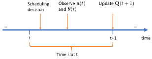
Figure 1. Sequence of events in one time slot.

We assume a general wireless interference model. Denote by $\mathcal{M}$ the set of all admissible link activations and, at time slot $t$, by $\mathbf{x}(t)=\{x_{e}(t)\}_{e\in E}\in\mathcal{M}$ the scheduling decision of whether to activate link $e\in E$:

$$x_{e}(t)=\begin{cases}1\text{, if $e$ is activated at time $t$}&\\ 0\text{, if $e$ is not activated at time $t$}\end{cases}.$$

We impose no structural restriction on the set $\mathcal{M}$, thereby capturing a wide range of practical wireless models including primary interference (Joo et al., 2009), k-hop interference (Joo et al., 2008), and protocol interference (Che et al., 2010). Let $\theta_{e}(t)$ be the service capacity of link $e$ at time slot $t$, which is bounded by a finite number, i.e. $\theta_{e}(t)\leq\mu_{max}$. For any link $e\in E$, we assume that $\{\theta_{e}(t)\}_{t\geq 0}$ are independent and that the mean service rate $\mu_{e}(t)=\mathbb{E}[\theta_{e}(t)]$ may vary over time. Additionally, we requires the mean service rate to be lower bounded by a strictly positive constant, i.e. $\mu_{e}(t)\geq\mu_{min}>0$; this assumption is also often imposed by the literature on optimal control of queueing systems with time-varying statistics (Freund et al., 2022; Yang et al., 2022). The effective service rate of link $e$ at time slot $t$ is then given by:

(1) $$b_{e}(t)=x_{e}(t)\theta_{e}(t),$$

which characterizes the achievable data rate of the link.

Let $Q_{e}(t)$ be the physical queue of backlogged packets at link $e\in E$ that are waiting to be transmitted at the end of time slot $t$. Since any link $e$ receives $a_{e}(t)$ packet arrivals and can serve at most $b_{e}(t)$ packets during a time slot, the queueing dynamics evolves as:

(2) $$Q_{e}(t+1)=\big{(}Q_{e}(t)+a_{e}(t)-b_{e}(t)\big{)}^{+},\quad\forall e\in E,$$

where $[x]^{+}=\max\{x,0\}$.

In order to capture the realistic characteristics of modern wireless network, we incorporate the following requirements in our model:

• Partial Observability: For every link $e\in E$, both the instantaneous packet arrivals $a_{e}(t)$ and link’s service capacity $\theta_{e}(t)$ are not available at the start of the time slot $t$ and thus cannot be used for making the scheduling decisions. At the end of time slot $t$, however, the nodes can accumulate statistics of the past time slot to obtain the packet arrivals $a_{e}(t)$’s and the service capacities of the activated links, i.e. those $\theta_{e}(t)$’s such that $x_{e}(t)=1$. For unactivated links $e$ where $x_{e}(t)=0$, though the information of $\theta_{e}(t)$ is not revealed, the effective service rate is $b_{e}(t)=0$. Thus, given the knowledge of $a_{e}(t)$ and $b_{e}(t)$, the queuing dynamics (2) for the next time slot $t+1$ can always be evaluated at the end of time slot $t$. The sequence of events within time slot $t$ is depicted in Figure 1.

• Non-Stationary Dynamics: We assume that both the mean packet arrivals $\boldsymbol{\lambda}(t)=(\lambda_{e}(t))_{e\in E}$ and service rates $\boldsymbol{\mu}(t)=(\mu_{e}(t))_{e\in E}$ vary over time, i.e. non-stationary.

• Unknown Statistics: All the statistics $\{\boldsymbol{\lambda}(t)\}_{t\geq 0}$ and $\{\boldsymbol{\mu}(t)\}_{t\geq 0}$ are unknown to the scheduler for making control decisions.

2.2. Asymptotic Relationships and Notations

Let $\mathbf{Q}(t)=(Q_{e}(t))_{e\in E}$, $\mathbf{a}(t)=(a_{e}(t))_{e\in E}$, $\boldsymbol{\theta}(t)=(\theta(t))_{e\in E}$ and $\mathbf{b}(t)=(b_{e}(t))_{e\in E}$ be respectively the vector of queue lengths, packet arrivals, service capacities and effective service rates. For any two real numbers $x$ and $y$, we let $x\vee y=\max\{x,y\}$ and $x\wedge y=\min\{x,y\}$. For any vector $\mathbf{x}=(x_{i})$ of real numbers and $p\in[1,\infty)$, we denote $\|\mathbf{x}\|_{p}$ as its $\ell_{p}$-norm. For the two cases of $p\in\{1,\infty\}$ used in this paper, we have $\|\mathbf{x}\|_{1}=\sum_{i}|x_{i}|$ and $\|\mathbf{x}\|_{\infty}=\max_{i}\{|x_{i}|\}$. For two positive multivariate functions $f(\mathbf{x})$ and $g(\mathbf{x})$, their asymptotic relationships (Cormen et al., 2009) are given in Table 1.

Table 1. Asymptotic Relationships

$f(\mathbf{x})=O(g(\mathbf{x}))$	there exists constants $M$ and $C$ such that
	$|f(\mathbf{x})|\leq C|g(\mathbf{x})|$ for all $\mathbf{x}$ with $\|\mathbf{x}\|_{\infty}>M$.
$f(\mathbf{x})=\Omega(g(\mathbf{x}))$	there exists constants $M$ and $C$ such that
	$|f(\mathbf{x})|\geq C|g(\mathbf{x})|$ for all $\mathbf{x}$ with $\|\mathbf{x}\|_{\infty}>M$.
$f(\mathbf{x})=\Theta(g(\mathbf{x}))$	$f(\mathbf{x})=O(g(\mathbf{x}))$ and $f(\mathbf{x})=\Omega(g(\mathbf{x}))$.
$f(\mathbf{x})=o(g(\mathbf{x}))$	for every $\varepsilon>0$, there exists constant $M$
	such that $|f(\mathbf{x})|\leq\varepsilon|g(\mathbf{x})|$ for all $\mathbf{x}$ with
	$\|\mathbf{x}\|_{\infty}>M$. In this case, we alternatively
	say $f(\mathbf{x})$ is sub-linear in $g(\mathbf{x})$.

2.3. Policy Space and Problem Statement

For any variable affected by the control of the scheduling decisions, we add the superscript $\pi$ to acknowledge that it is under the action of the policy $\pi$. An admissible policy $\pi$ at every time slot $t$ generates a scheduling decision $\mathbf{x}^{\pi}(t)\in\mathcal{M}$ using only the knowledge of the past packet arrivals $\mathbf{a}(0),\mathbf{a}(1),...,\mathbf{a}(t-1)$, the past effective service rates $\mathbf{b}(0),\mathbf{b}(1),...,\mathbf{b}(t-1)$, and the past decisions $\mathbf{x}(0),\mathbf{x}(1),...,\mathbf{x}(t-1)$ up to time $t-1$. Additionally, we consider idealized policies, the definition of which is similar to that of an admissible policy except that at time slot $t$, it also has the full knowledge of the network statistics $\boldsymbol{\lambda}(t)$ and $\boldsymbol{\mu}(t)$ and can use them in making the scheduling decisions. The set of all admissible policies and the set of all idealized polices are respectively denoted by $\Pi$ and $\Pi_{s}$. Under the simplified model whereby the network dynamics are stationary, (Stahlbuhk et al., 2019) designed a joint learning and scheduling algorithm in $\Pi$ that supports the same stability region, i.e. the set of arrival rates under which the system is stabilizable, as that of idealized policies in $\Pi_{s}$. Nevertheless, generalization to the case of non-stationary network dynamics is non-trivial due to the analytical intractability of the capacity region. Moreover, the only previous work (Yang et al., 2022) that attempts to learn non-stationary network dynamics could achieve only a reduced stability region that is constrained by the window-based dynamics, thereby being sub-optimal.

In this paper, we aim to develop a control scheme for the class of policies in $\Pi$ that maximizes the stability region of the network under our considered setting.

3. Notion of Stability for Non-Stationary Network with Unknown Statistics

One main challenge of non-stationary network control is that the analytical characterization of the capacity region for the case of stationary network may no longer hold under the non-stationarity. In this Section, we propose a new notion of throughput-optimality that is more suitable to the non-stationary setting. For the simplified case of stationary network, we further establish the equivalence between our new notion and the conventional notion of throughput-optimality.

3.1. Assumption on Non-Staionary Dynamics

For any $t_{1}<t_{2}$, we denote the total variation of the mean service rate by:

(3) $$\gamma(t_{1},t_{2})=\sum_{t=t_{1}+1}^{t_{2}}\|\boldsymbol{\mu}(t)-\boldsymbol{\mu}(t-1)\|_{\infty},$$

and stipulate the following mild assumption on the non-stationarity of the mean service rates.

Assumption 1.

For any $t_{1}<t_{2}$, the total variation is upper-bounded by $\gamma(t_{1},t_{2})=O(|t_{2}-t_{1}|^{\alpha})$ for some $\alpha\in[0,1)$.

Our assumption only requires the total variation of mean service rates over any time period to grow sub-linearly in time, thereby ensuring that the network dynamics do not vary too aggressively. Similar assumptions have been extensively used the literature of learning in non-stationary environments (Chen et al., 2020; Wei et al., 2016; Besbes et al., 2014).

3.2. Performance Metrics

Before characterizing the stability regions of interest, we first define the $Q_{T}$ measure that captures the growth of queue size in expectation, and present the equivalent definition of mean rate stability (Neely, 2010) under the $Q_{T}$ measure.

Definition 0 ($Q_{T}$ Measure).

The total expected queue length at time $T$ under a control of policy $\pi$ is quantified by $Q^{\pi}_{T}=\mathbb{E}\big{[}\sum_{e\in E}Q^{\pi}_{e}(T)\big{]}$.

Definition 0 (Mean Rate Stability).

A network is mean rate stable under a policy $\pi$ if:

$$\lim_{T\to\infty}\frac{\mathbb{E}[\sum_{e\in E}Q^{\pi}_{e}(T)]}{T}=0,$$

or equivalently $Q_{T}^{\pi}=o(T)$.

The notion of stability region of a policy $\pi$ describes the set of arrival rate vectors such that mean rate stability could be achieved under $\pi$. The stability region $\mathbf{\Lambda}$ is the region that can be achieved by the class $\Pi$ of admissible policies, as formally defined below.

Definition 0 (Stability Region).

The stability region of the class of admissible policies is defined as:

$$\mathbf{\Lambda}=\big{\{}\{\boldsymbol{\lambda}(t)\}_{t\geq 0}:\exists\pi\in\Pi\text{ such that }Q_{T}^{\pi}=o(T)\big{\}}.$$

Similarly, we define the idealized stability region $\mathbf{\Lambda}_{s}$ of the class $\Pi_{s}$ of idealized policies.

Definition 0 (Idealized Stability Region).

The stability region of the class of idealized policies is defined as:

$$\mathbf{\Lambda}_{s}=\big{\{}\{\boldsymbol{\lambda}(t)\}_{t\geq 0}:\exists\pi\in\Pi_{s}\text{ such that }Q_{T}^{\pi}=o(T)\big{\}}.$$

Note that we always have $\mathbf{\Lambda}\subseteq\mathbf{\Lambda}_{s}$, since the idealized policies have the full network statistics as opposed to the admissible policies. For the simplified model of stationary dynamics, a special case of our setting where Assumption 1 trivially holds with $\alpha=0$, (Stahlbuhk et al., 2019) designed an admissible policy stabilizing any arrival rate vector in $int(\mathbf{\Lambda}_{s})$, i.e. the interior of the idealized stability region. The algorithmic development and analysis of (Stahlbuhk et al., 2019) heavily rely on the fact that under the stationary dynamics whereby $\boldsymbol{\lambda}=\boldsymbol{\lambda}(t)$ and $\boldsymbol{\mu}=\boldsymbol{\mu}(t)$ for all $t\geq 0$, the idealized stability region $\mathbf{\Lambda}_{s}$ can be further characterized by the existence of a policy $\pi^{*}\in\Pi_{s}$ such that:

(4) $$\lambda_{e}=\lim_{T\to\infty}\frac{1}{T}\sum_{t=0}^{T-1}a_{e}(t)\leq\lim_{T\to\infty}\frac{1}{T}\sum_{t=0}^{T-1}b^{\pi^{*}}_{e}(t),\text{ }\forall e\in E.$$

However, under non-stationarity, the above limits may not even exist, thereby hindering the adoption of stability region’s characterization as in the case of stationary dynamics. Such analytical intractability of the stability region is central to the problem of optimal control for non-stationary network (Andrews and Zhang, 2004; Liang and Modiano, 2018).

3.3. Notion of Throughput-Optimality for Non-Stationary Network

In this Section, we propose a novel notion of throughput-optimality for non-stationary networks. For the simplified setting of stationary network, the conventional notion of stability defines a policy $\pi$ to be throughput-optimal if it can stabilize the system for any arrival rate $\boldsymbol{\lambda}\in int(\mathbf{\Lambda}_{s})$, i.e. in the interior of the idealized stability region. This is equivalent to $\boldsymbol{\lambda}\in(1-\varepsilon)\mathbf{\Lambda}_{s}$ for some $\varepsilon>0$, which is then usually incorporated with the analytical characterization of $\mathbf{\Lambda}_{s}$ for establishing the stability of MaxWeight-type algorithms. However, in the context of non-stationary networks, such an approach may not be directly applicable due to the analytical intractability of the idealized stability region $\mathbf{\Lambda}_{s}$. To this end, we first present our new definition of approximate stability region, which is central to our throughput-optimality notion and algorithmic development.

Definition 0 (Approximate Stability Region).

Given any $\beta\in[0,1]$, we define the approximate region $\mathbf{\Lambda}_{s}(\beta)$ as:

$$\mathbf{\Lambda}_{s}(\beta)=\big{\{}\{\boldsymbol{\lambda}(t)\}_{t\geq 0}:\exists\pi\in\Pi_{s}\text{ such that }Q_{T}^{\pi}=O\big{(}T^{\beta}\big{)}\big{\}}$$

We now derive the key properties of $\mathbf{\Lambda}_{s}(\beta)$ and its relation to the idealized stability region $\mathbf{\Lambda}_{s}$ in the following Lemma, whose proof is deferred to Appendix A.

Lemma 0.

The set $\mathbf{\Lambda}_{s}(\beta)$ is expanding for increasing $\beta$, i.e. if $0\leq\beta_{1}\leq\beta_{2}\leq 1$, then $\mathbf{\Lambda}_{s}(\beta_{1})\subseteq\mathbf{\Lambda}_{s}(\beta_{2})$. Moreover, for any $\beta\in[0,1)$, we have $\mathbf{\Lambda}_{s}(\beta)\subseteq\mathbf{\Lambda}_{s}\subseteq\mathbf{\Lambda}_{s}(1)$.

Lemma 6 suggests that the region $\mathbf{\Lambda}_{s}(\beta)$ grows arbitrarily close to $\mathbf{\Lambda}_{s}$ as $\beta$ approaches $1$. Moreover, leveraging this notion of approximate stability region, the next Theorem establishes the characterization of the true stability region $\mathbf{\Lambda}$.

Theorem 7.

Under Assumption 1, we have the following characterization of the stability region:

$$\mathbf{\Lambda}_{s}(\beta)\subseteq\mathbf{\Lambda}\subseteq\mathbf{\Lambda}_{s},$$

for any $\beta\in[0,1)$.

Proof.

As the idealized policies have the full network statistics as opposed to the admissible policies, the idealized stability region $\mathbf{\Lambda}_{s}$ trivially subsumes the stability region $\mathbf{\Lambda}$. The proof of $\mathbf{\Lambda}_{s}(\beta)\subseteq\mathbf{\Lambda}$ is based on our development of the admissible policy MW-UCB in Section 4 that, given any $\beta\in[0,1)$, achieves mean rate stability for any set of arrival rates $(\boldsymbol{\lambda}(t))_{t\geq 0}\in\mathbf{\Lambda}_{s}(\beta)$ (Theorem 3). ∎

Motivated by Theorem 7, we propose the following notion of throughput-optimality for non-stationary network control.

Definition 0 (Throughput-Optimality).

A policy $\pi\in\Pi$ is throughput optimal if given any $\beta\in[0,1)$, the network under $\pi$ is mean rate stable for any $\{\boldsymbol{\lambda}(t)\}_{t\geq 0}\in\mathbf{\Lambda}_{s}(\beta)$.

Under the above definition, we aim to develop an admissible policy in $\Pi$ that is throughput-optimal for our considered setting of non-stationary and partially-observable network.

3.4. Connection to Traditional Notion of Throughput-Optimality for Stationary Networks

We further demonstrate the equivalence of our throughput-optimality notion to the usual notion in the case of stationary network whereby $\boldsymbol{\lambda}=\boldsymbol{\lambda}(t)$ and $\boldsymbol{\mu}=\boldsymbol{\mu}(t)$ for all $t\geq 0$. As discussed in Section 3.2, the idealized stability region $\mathbf{\Lambda}_{s}$ can be characterized by:

$$\bar{\mathbf{\Lambda}}_{s}=\big{\{}\boldsymbol{\lambda}:\exists\pi^{*}\in\Pi_{s}\text{ such that $\pi^{*}$ satisfies \eqref{stationary_equation}}\big{\}},$$

and an admissible policy is throughput-optimal (in the usual notion) if it can stabilize any arrival rate $\boldsymbol{\lambda}\in\bar{\mathbf{\Lambda}}_{s}$. The next Theorem illustrates that our new notion of throughput-optimality implies the usual notion of throughput-optimality in the stationary network control problem.

Theorem 9.

Under the stationary network setting, if a policy $\pi\in\Pi$ is throughput-optimal according to Definition 8, then the network under $\pi$ is mean rate stable for any $\boldsymbol{\lambda}\in\bar{\mathbf{\Lambda}}_{s}$.

Proof Sketch. Given $\boldsymbol{\lambda}\in\bar{\mathbf{\Lambda}}_{s}$, we can show via Lyapunov drift analysis that the Max-Weight (MW) policy with full knowledge of the statistics achieves $Q_{T}^{\textsc{MW}}=O\big{(}T^{\frac{1}{2}}\big{)}$. Consequently, this implies that $\boldsymbol{\lambda}\in\mathbf{\Lambda}_{s}(\frac{1}{2})$. Since by our Definition 8, a throughput-optimal policy $\pi$ would support the stability region $\mathbf{\Lambda}_{s}(\frac{1}{2})$, it thus guarantees mean rate stability for any $\boldsymbol{\lambda}\in\bar{\mathbf{\Lambda}}_{s}$. The full proof is given in Appendix B.

4. Scheduling with non-stationary and unknown channel statistics

In this Section, we present MW-UCB as a provably throughput-optimal policy for non-stationary network control. We provide the preliminaries of Upper-Confidence Bound (UCB) for learning uncertain channel statistics in Section 4.1 and the algorithmic development of MW-UCB in Section 4.2. The throughput-optimality and stability results of MW-UCB then follow in Section 4.3.

4.1. Upper-Confidence Bound (UCB) for Learning Uncertain Channel Statistics

Central to our problem is the learning of not only the unknown links’ service rates but also the scheduling decisions that can maximize the overall network’s throughput. We start by considering a simplistic problem setting in which the network dynamics are stationary and the objective is to attain the maximum possible total service capacity (in expectation) of the network, and show that a simple Upper-Confidence Bound (UCB) algorithm is close-to-optimal in this scenario. However, while having the potential for being the solution for network control under uncertain channel statistics, the UCB algorithm in its original form lacks the adaptivity to deal with non-stationary dynamics and is a pure learning scheme in nature, which is not designed to deal with sophisticated control tasks as in our original problem.

4.1.1. A Simplistic Problem Setting and Application of UCB

At any time slot $t$, the scheduling decision $\mathbf{x}(t)$ yields in expectation the service of $\mu_{e}(t)x_{e}(t)$ for link $e\in E$ and thus the total service of:

(5) $$\sum_{e\in E}\mu_{e}(t)x_{e}(t).$$

Now, we turn into a simplified objective of maximizing the total service (5) over the time horizon $T$ of the network and further assume stationary dynamics of the links’ service rates, i.e. $\mu_{e}(t)=\mu_{e},\forall e\in E,t\geq 0$. Under this setting, an idealized policy with full knowledge of the statistics $\boldsymbol{\mu}=(\mu_{e})_{e\in E}$ would make the scheduling decision at every time slot $t$ that maximizes (5), i.e.

(6) $$\mathbf{x}(t)=\mathbf{x}^{*}=\operatorname*{\arg\!\max}_{\mathbf{x}\in\mathcal{M}}\big{\{}\sum_{e\in E}\mu_{e}x_{e}\big{\}}.$$

However, such statistics $\boldsymbol{\mu}=(\mu_{e})_{e\in E}$ are unknown in practice and thus must be learned, under our requirement of partial observability, via samples of service capacities of links having been activated. This gives rise to the exploration/exploitation tradeoff, where the controller must simultaneously learn the channel statistics $\boldsymbol{\mu}$ and utilize the existing information of observed service capacities to schedule transmissions achieving high total throughput. In particular, the problem of solving (6) over the time horizon $T$ can be characterized as combinatorial multi-armed bandit (CMAB) with linear reward in stationary environment, which can be addressed by the class of UCB algorithms (Auer et al., 2002; Gai et al., 2012; Kveton et al., 2015). We hereby consider the UCB algorithm in (Kveton et al., 2015), which proceeds as follows. At any time slot $t$ and for every edge $e\in E$, the UCB algorithm keeps track of $T_{t}(e)$ and $\hat{\theta}_{e}(t)$, which respectively correspond to the number of times link $e$ has been activated and observed up to time $t$, and the empirical mean of all the observations of the service capacities, i.e. those $\theta_{e}(s)$ such that $x_{e}(s)=1$ for $s\in[0,t)$. The UCB weights are computed according to:

$$U_{e}(t)=\hat{\theta}_{e}(t)+\sqrt{\frac{3\log(t)}{2T_{t}(e)}},\forall e\in E,$$

which are then used for constructing the scheduling decision as:

(7) $$\mathbf{x}(t)=\operatorname*{\arg\!\max}_{\mathbf{x}\in\mathcal{M}}\big{\{}\sum_{e\in E}U_{e}(t)x_{e}\big{\}}.$$

The total difference in achievable total expected service capacity between the maximizing policy with the full knowledge of the statistics $\boldsymbol{\mu}$ that makes the decision $\mathbf{x}^{*}$ as in (6) and the UCB algorithm that makes the decision $\mathbf{x}(t)$ as in (7) is captured by the regret:

(8) $$\mathcal{R}_{0}(T)=T\sum_{e\in E}\mu_{e}x^{*}_{e}-\sum_{t=0}^{T-1}\sum_{e\in E}\mu_{e}x_{e}(t).$$

This type of metrics is also used by (Stahlbuhk et al., 2019) for characterizing the performance and exploration/exploitation tradeoff of their joint learning and scheduling algorithm. From (Kveton et al., 2015, Theorem 5), we have $\mathcal{R}_{0}(T)=O\big{(}\log(T)\big{)}$, which guarantees only logarithmic growth in total error if the UCB algorithm is applied. Moreover, this regret bound is asymptotically tight (Kveton et al., 2015, Proposition 1).

4.1.2. Limitations of The Conventional UCB Algorithm

While attaining competitive performance in the simplistic problem setting, the conventional UCB algorithm lacks the generality to readily be extended to deal with our problem of interest. First, vanilla UCB is known to be inappropriate for handling non-stationary dynamics (Hartland et al., 2007). Second, the formulation (6) that permits the adoption of UCB as a direct solution does not take into account the control of the system under arbitrary arrival rates: for example, if a policy aims to attain the maximum possible total service and hence always makes the scheduling decision $\mathbf{x}^{*}$ as in (6), it would inevitably overload certain unactivated links, i.e. $e\in E$ with $x^{*}_{e}=0$, to which there are packet arrivals over time. On the other hand, the Max-Weight policy (Neely, 2010; Tassiulas and Ephremides, 1992) that incorporates the queue lengths into making scheduling decision can adapt to the dynamics of arbitrary arrival rates. Consequently, the solution for scheduling in non-stationary wireless networks with partial observability and unknown statistics requires the interplay between learning and network control. In the next Section, we present our main algorithm that combines the Max-Weight policy with UCB to address these aforementioned challenges through its joint learning and scheduling scheme.

4.2. The MW-UCB Algorithm

We proceed to develop our scheduling algorithm, termed MW-UCB, based on a frame-based variant (Stahlbuhk et al., 2019) of the Max-Weight policy (Neely, 2010; Tassiulas and Ephremides, 1992) and the augmentation of the sliding-window UCB (Chen et al., 2020) in the weight construction for adaptively learning the channels’ statistics under non-stationarity. The full MW-UCB policy is depicted in Algorithm 1 with the convention that $0/0=0$.

Input: graph $\mathcal{G}(V,E)$, restart period $\tau$, window size $d\leq\tau$

1 for $t=1,...,T$ do

2       if $t=\tau_{j}\in\mathcal{T}=\{\tau_{0},\tau_{1},...,\tau_{K}\}$ then

3             Initialize $\phi_{e}(\tau_{j})=0,N_{e}(\tau_{j})=0,\hat{\mu}_{e}(t)=0,\forall e\in E$

4             Reset the weights: $w_{e}(\tau_{j})=\frac{Q_{e}(\tau_{j})}{\|\mathbf{Q}(\tau_{j})\|_{\infty}},\forall e\in E$

5            

6       end if

7      if $t\in(\tau_{j},\tau_{j+1})$ then

8             for $e\in E$ do

9                   $\phi_{e}(t)=\phi_{e}(t-1)-\mathbbm{1}_{\{t\geq\tau_{j}+d\}}b_{e}(t-d)+b_{e}(t-1)$

10                   $N_{e}(t)=N_{e}(t)-\mathbbm{1}_{\{t\geq\tau_{j}+d\}}x_{e}(t-d)+x_{e}(t-1)$

11                   $\hat{\mu}_{e}(t)=\frac{\phi_{e}(t)}{N_{e}(t)}$ $\triangleright$ empirical estimate of $\mu_{e}(t)$

12                   $w_{e}(t)=w_{e}(\tau_{j})$ $\triangleright$ fixing queue lengths

13                  

14             end for

15            

16       end if

17      $\rho_{e}(t)=\sqrt{\frac{3\log(\tau)}{2N_{e}(t)}}\text{ (or $\infty$ if $N_{e}(t)=0$)},\forall e\in E$

18      $\bar{W}_{e}(t)=\min\{w_{e}(t)\hat{\mu}_{e}(t)+\rho_{e}(t),1\},\forall e\in E$ $\triangleright$ computing UCB weights

19      

20      [Scheduling] Activate the link activation vector: $\mathbf{x}(t)=\operatorname*{\arg\!\max}_{\mathbf{x}\in\mathcal{M}}\big{\{}\sum_{e\in E}\bar{W}_{e}(t)x_{e}\big{\}}$

21       Observe $\mathbf{a}(t)$ and $\mathbf{b}(t)$, and update the queues: $Q_{e}(t+1)=\big{(}Q_{e}(t)+a_{e}(t)-b_{e}(t)\big{)}^{+},\quad\forall e\in E,$

22 end for

Algorithm 1 Max-Weight with UCB (MW-UCB)

For the class of idealized policies in $\Pi_{s}$, the Max-Weight policy (Neely, 2010) that at time slot $t$ weights each edge $e$ by $Q_{e}(t)\mu_{e}(t)$ and consequently schedule the link activation vector according to:

(9) $$\mathbf{x}(t)=\operatorname*{\arg\!\max}_{\mathbf{x}\in\mathcal{M}}\big{\{}\sum_{e\in E}Q_{e}(t)\mu_{e}(t)x_{e}\big{\}}$$

is known to be throughput-optimal for the case of stationary network (Stahlbuhk et al., 2019; Neely, 2010) and obtains competitive performance on adversarial network control (Liang and Modiano, 2018). Nevertheless, under our considered model, the vector $\boldsymbol{\mu}(t)$ of mean service rates is unknown a priori, thereby hindering any direct adoption of the Max-Weight policy. The algorithmic design for joint network control and learning of the weights $\{Q_{e}(t)\mu_{e}(t)\}_{e\in E}$ faces two challenges. First, $Q_{e}(t)\mu_{e}(t)$ is time-varying due to the dynamics of the queue length $Q_{e}(t)$ and the non-stationarity of $\mu_{e}(t)$. Second, the evolution of the weight $Q_{e}(t)\mu_{e}(t)$ is coupled with the scheduling decision $\mathbf{x}(t)$ due to its interdependence with effective service rate via (1) and thus the queueing dynamics (2). To address these challenges, we periodically freeze the queue length information in the weight instantiation, which helps to alleviate a source of non-stationarity and decouples the weight evolution from the scheduling decision. Specifically, our method partitions the time horizon $T$ into frames of size $\tau$, where the $j^{th}$ frame begins at time slot $\tau_{j}=j\tau$, called restart point. We allow the last frame to have size potentially less than $\tau$ and let $\mathcal{T}=\{\tau_{0},\tau_{1},...,\tau_{K}\}$ be the set of all restart points, i.e. $K$ is the largest number such that $\tau_{K}<T$. Then for any $t\in[\tau_{j},\tau_{j+1})$, we use the normalized queue backlogs at the restart point $\tau_{j}$ as the unified weights (Line 1 and Line 1 of Algorithm 1):

(10) $$w_{e}(\tau_{j})=\frac{Q_{e}(\tau_{j})}{\|\mathbf{Q}(\tau_{j})\|_{\infty}},\forall e\in E,$$

and aim to solve the following ”relaxed” problem of (9) with simplified time-varying weight structure:

(11) $$\mathbf{x}(t) =\operatorname*{\arg\!\max}_{\mathbf{x}\in\mathcal{M}}\big{\{}\sum_{e\in E}Q_{e}(\tau_{j})\mu_{e}(t)x_{e}\big{\}}$$

(12) $$\overset{\eqref{normalized_weight1}}{=}\operatorname*{\arg\!\max}_{\mathbf{x}\in\mathcal{M}}\big{\{}\sum_{e\in E}w_{e}(\tau_{j})\mu_{e}(t)x_{e}\big{\}}.$$

Note that the objective in (11) is the ”approximation” of the objective in (9) with error growing linearly in $\tau$. Moreover, the problem of solving (12) over $\tau$ time slots from $\tau_{j}$ to $\tau_{j+1}-1$ can be characterized as stochastic combinatorial multi-armed bandit (SCMAB) problem in non-stationary environment, whereby the mean reward of each arm, i.e. $w_{e}(\tau_{j})\mu_{e}(t)$, varies over time and is independent of the action, i.e. scheduling decision. To this end, we adopt the combinatorial UCB with sliding window (CUCB-SW) algorithm (Chen et al., 2020) for dealing with SCMAB under non-stationarity. Specifically, CUCB-SW is restarted at the beginning of each frame with the newly updated queue weights for the joint learning of the mean service rates $\boldsymbol{\mu}(t)$’s and control of the system. Given the sliding window of size $d$ as a hyper-parameter to be chosen later, the algorithm computes the estimate $\hat{\mu}_{e}(t)$ of the true mean service rate $\mu_{e}(t)$ as the local empirical average of the observed service capacities in the last $d$ time slots. Formally, for $t\in[\tau_{j},\tau_{j+1})$, i.e. within the $j^{th}$ frame, and any $e\in E$, the following quantities:

(13) $$\phi_{e}(t)=\sum_{s=\tau_{j}\vee(t-d)}^{t-1}\mathbbm{1}_{\{x_{e}(s)=1\}}\theta_{e}(s)=\sum_{s=\tau_{j}\vee(t-d)}^{t-1}b_{e}(s),$$

(14) $$N_{e}(t)=\sum_{s=\tau_{j}\vee(t-d)}^{t-1}\mathbbm{1}_{\{x_{e}(s)=1\}}=\sum_{s=\tau_{j}\vee(t-d)}^{t-1}x_{e}(s),$$

respectively denote the total observed service capacities of link $e$ and the number of times it had been activated up to time $t-1$ over the last $d$ time slots. Line 1 and Line 1 of Algorithm 1 equivalently rewrite (13) and (14) in recursive forms for actual iterative updates in the algorithm. Then the local empirical average can be computed accordingly via $\hat{\mu}_{e}(t)={\phi_{e}(t)}/{N_{e}(t)}$ as in Line 1. Finally, the UCB weights are computed by (Line 1):

$$\bar{W}_{e}(t)=\min\bigg{\{}w_{e}(\tau_{j})\hat{\mu}_{e}(t)+\sqrt{\frac{3\log(\tau)}{2N_{e}(t)}},1\bigg{\}},\forall e\in E,$$

to be used for constructing of the scheduling decision (Line 1) as:

(15) $$\mathbf{x}(t)=\operatorname*{\arg\!\max}_{\mathbf{x}\in\mathcal{M}}\big{\{}\sum_{e\in E}\bar{W}_{e}(t)x_{e}\big{\}}.$$

In order to capture the loss due to learning when CUCB-SW is applied to solve (12) within the $j^{th}$ frame, we consider the regret:

$$\mathcal{R}(\tau_{j}) =\sum_{t=\tau_{j}}^{\tau_{j+1}-1}\max_{\mathbf{x}\in\mathcal{M}}\sum_{e\in E}w_{e}(\tau_{j})\mu_{e}(t)x_{e}$$

(16) $$\quad-\sum_{t=\tau_{j}}^{\tau_{j+1}-1}\sum_{e\in E}w_{e}(\tau_{j})\mu_{e}(t)x_{e}(t),$$

which characterizes the gap in objective between the maximizing policy with the full knowledge of the statistics $\boldsymbol{\mu}(t)$ for $t\in[\tau_{j},\tau_{j+1})$ that solves (12) and the considered policy that solves (15). The following Lemma 1, whose proof is given in Appendix D.3, provides an upper bound for $\mathcal{R}(\tau_{j})$.

Lemma 0.

Under MW-UCB, the regret $\mathcal{R}(\tau_{j})$ can be bounded by:

$$\mathcal{R}(\tau_{j}) \leq|E|\bigg{(}\frac{\tau}{d}+1\bigg{)}\bigg{(}2\sqrt{6\log(\tau)}+48\sqrt{d}\log(\tau)\bigg{)}$$

$$\quad+4|E|d\cdot\gamma(\tau_{j},\tau_{j+1})+|E|\frac{\tau}{\sqrt{d}}+\frac{\pi^{2}}{3}|E|^{2}\mu_{max}$$

$$\quad+\frac{\pi^{2}}{6}|E|^{2}\mu_{max}\log\big{(}2d^{1/2}\big{)}.$$

Under Assumption 1, which gives $\gamma(\tau_{j},\tau_{j+1})=O(\tau^{\alpha})$, and by setting $d=\Theta\big{(}\tau^{\frac{2}{3}(1-\alpha)}\big{)}$, we further have $\mathcal{R}(\tau_{j})=O\big{(}\log(\tau)\tau^{\frac{1}{3}(\alpha+2)}\big{)}$.

The guarantee in Lemma 1 demonstrates that the average loss due to learning over $\tau$ time slots of the $j^{th}$ frame vanishes as $\tau$ grows in the sense that $\frac{\mathcal{R}(\tau_{j})}{\tau}\to 0$ as $\tau\to\infty$ under our mild assumption on the learnability of the system. This is crucial for establishing the throughput-optimality of MW-UCB in the next Section.

4.3. Throughput-Optimality and Stability Results

In this Section, we prove the throughput-optimality of MW-UCB and, as a byproduct, its strong stability in a region constrained by window-based dynamics. The key components of the proof leverage the regret bound for learning non-stationarity (Lemma 1) in the analysis of the frame-based Lyapunov drift and non-trivially generalize the shedding technique from the adversarial network control literature (Liang and Modiano, 2018). In particular, to address the analytical intractability of the capacity region, we shed the traffic of the original system to obtain a new imaginary system whose traffic is within the window-based region, which is formally described in Definition 2. While the shedding process incurs additional term in the queue bound as a tradeoff, it makes the imaginary network dynamics tractable, from which stability of MW-UCB can be derived.

Definition 0 (Window-Based Region).

The window-based region $\mathcal{C}(W,\varepsilon)$ of the class of idealized policies is defined as:

$$\mathcal{C}(W,\varepsilon)=\big{\{} \{\boldsymbol{\lambda}(t)\}_{t\geq 0}:\exists\pi\in\Pi_{s}\text{ such that for $q=0,W,2W,...$}$$

$$\sum_{t=q}^{q+W-1}\lambda_{e}(t)\leq(1-\varepsilon)\sum_{t=q}^{q+W-1}\mathbb{E}[b^{\pi}_{e}(t)],\text{ }\forall e\in E\big{\}}.$$

Specifically, the sequence of arrival rates $\{\boldsymbol{\lambda}(t)\}_{t\geq 0}$ satisfies the window-based region, parameterized by window size $W$ and a shrinkage term $\varepsilon$, if there exists an idealized policy such that the total mean arrivals are less than a fraction $1-\varepsilon$ of the total mean services over a window of $W$ slots starting at every starting point $t=0,W,2W,...$ Next, we proceed to establish the main Theorem on the throughput-optimality of MW-UCB.

Theorem 3.

Under Assumption 1, MW-UCB is throughput-optimal.

Proof.

Given any $\beta\in[0,1)$, we show that MW-UCB can achieve mean rate stability for any $\{\boldsymbol{\lambda}(t)\}_{t\geq 0}\in\mathbf{\Lambda}_{s}(\beta)$. We now consider an imaginary system that is obtained by imitating the same link service process $\{\boldsymbol{\theta}(t)\}_{t\geq 0}$ as the original system’s and shedding a certain amount of traffic from the original system’s arrivals $\{\mathbf{a}(t)\}_{t\geq 0}$ to obtain a new sequence of arrivals $\{\tilde{\mathbf{a}}(t)\}_{t\geq 0}$ with $\tilde{\lambda}_{e}(t)=\mathbb{E}[\tilde{a}_{e}(t)],\forall e\in E,t\geq 0$. Denote the amount of shed traffic within the time horizon by:

(17) $$X_{T}=\sum_{t=0}^{T-1}\sum_{e\in E}a_{e}(t)-\sum_{t=0}^{T-1}\sum_{e\in E}\tilde{a}_{e}(t).$$

For some $\varepsilon\in(0,1)$ to be determined later, we consider the shedding scheme as in the following Lemma 4, whose proof is deferred to Appendix C.

Lemma 0.

Given $\{\boldsymbol{\lambda}(t)\}_{t\geq 0}\in\mathbf{\Lambda}_{s}(\beta)$ and any $\varepsilon\in(0,1)$, there exists a shedding procedure such that $\{\tilde{\boldsymbol{\lambda}}(t)\}_{t\geq 0}\in\mathcal{C}(\tau,\varepsilon)$ and:

(18) $$\mathbb{E}[X_{T}]=O\big{(}T^{\beta+1}\tau^{-1}+\varepsilon T+\tau\big{)}.$$

Intuitively, Lemma 4 suggests that, for analysis, despite the potential analytical intractability of the approximate region $\mathbf{\Lambda}_{s}(\beta)$, we can shed traffic to obtain an imaginary system that is constrained in $\mathcal{C}(\tau,\varepsilon)$ and thus more tractable with the tradeoff as characterized by (18). When MW-UCB is applied to the original system, it produces the sequence of decisions $\{\mathbf{x}^{\textsc{MW-UCB}}(t)\}_{t\geq 0}$. Let $\widetilde{\mathbf{Q}}(t)=\{\widetilde{Q}_{e}(t)\}_{e\in E}$ be the virtual queue length vector at time slot $t$ if such sequence of decisions $\{\mathbf{x}^{\textsc{MW-UCB}}(t)\}_{t\geq 0}$ is applied to the imaginary system. Then the following Lemma 5 upper-bounds the $Q_{T}$ measure of MW-UCB in the original system. The proof is given in Appendix D.1.

Lemma 0.

We have the following bound:

(19) $$Q_{T}^{\textsc{MW-UCB}}\leq\mathbb{E}[X_{T}]+\mathbb{E}\big{[}\sum_{e\in E}\widetilde{Q}_{e}(T)\big{]}.$$

In particular, though the shedding process incurs the term $\mathbb{E}[X_{T}]$, which can be bounded as in Lemma 4, in the queue bound of the original system, we are now left with bounding the virtual queues $\widetilde{\mathbf{Q}}(t)$ which evolve over the imaginary system that is more tractable. Next, we further provide guarantee for the total expected queue length of the imaginary system, i.e. the second term of (19), as follows.

Lemma 0.

Under Assumption 1 and given $\{\tilde{\boldsymbol{\lambda}}(t)\}_{t\geq 0}\in\mathcal{C}(\tau,\varepsilon)$, there exists some universal constant $c_{1}>0$ such that if $c_{1}\log(\tau)\tau^{\frac{1}{3}(\alpha-1)}\leq\varepsilon<1$, MW-UCB with $d=\Theta\big{(}\tau^{\frac{2}{3}(1-\alpha)}\big{)}$ being applied to the imaginary system satisfies:

(20) $$\mathbb{E}\big{[}\sum_{e\in E}\widetilde{Q}_{e}(T)\big{]}=O\big{(}T^{\frac{1}{2}}\tau^{\frac{1}{2}}+T^{1+\frac{\beta}{2}}\tau^{-\frac{1}{2}}+\varepsilon^{\frac{1}{2}}T\big{)}.$$

The proof of Lemma 6 can be found in Appendix D.2. Notice that under our assumption $\alpha<1$ (implying $\lim_{\tau\to\infty}\log(\tau)\tau^{\frac{1}{3}(\alpha-1)}=0$), without loss of generality (WLOG), we can consider $\tau$ large enough so that $c_{1}\log(\tau)\tau^{\frac{1}{3}(\alpha-1)}<1$. The requirement that the considered ”shrinkage” $\varepsilon$ must be bounded away from $0$ by such quantity reflects the loss due to learning. Note that the whole shedding process only serves for analytical purposes, i.e. we can shed the original system into the new imaginary system in the sense of Lemma 4 for any arbitrary $\varepsilon\in(0,1)$. Finally, by setting $\varepsilon=c_{1}\log(\tau)\tau^{\frac{1}{3}(\alpha-1)}$, we plug (18) and (20) into (19) to obtain the following bound for the $Q_{T}$ measure of MW-UCB with $d=\Theta\big{(}\tau^{\frac{2}{3}(1-\alpha)}\big{)}$:

$$Q_{T}^{\textsc{MW-UCB}} =O\big{(}T^{\beta+1}\tau^{-1}+T\sqrt{\log(\tau)}\tau^{\frac{1}{6}(\alpha-1)}+T^{1+\frac{\beta}{2}}\tau^{-\frac{1}{2}}+T^{\frac{1}{2}}\tau^{\frac{1}{2}}\big{)}.$$

Therefore, MW-UCB with $\tau=T^{\frac{1}{2}(\beta+1)}$ and $d=\Theta\big{(}\tau^{\frac{2}{3}(1-\alpha)}\big{)}$ can achieve:

$$Q_{T}^{\textsc{MW-UCB}} =O\big{(}T^{\frac{1}{2}(\beta+1)}+\sqrt{\log(T)}T^{1-\frac{1}{12}(\beta+1)(1-\alpha)}+T^{\frac{1}{4}(\beta+3)}\big{)}$$

(21) $$=o(T),$$

where the last line holds because $\alpha,\beta\in[0,1)$. Since (21) asserts the mean rate stability of MW-UCB for $\{\boldsymbol{\lambda}(t)\}_{t\geq 0}\in\mathbf{\Lambda}_{s}(\beta)$ given any $\beta\in[0,1)$, we conclude that MW-UCB is throughput-optimal. ∎

Additionally, we derive the strong stability of MW-UCB for the window-based region in the following Corollary, whose proof is given in Appendix E.

Corollary 0.

Under Assumption 1, MW-UCB with a fixed window size $\tau$ and $d=\Theta\big{(}\tau^{\frac{2}{3}(1-\alpha)}\big{)}$ achieves strong stability for any $\{{\boldsymbol{\lambda}}(t)\}_{t\geq 0}\in\mathcal{C}(\tau,\varepsilon)$ with any $\varepsilon>c_{1}\log(\tau)\tau^{\frac{1}{3}(\alpha-1)}$ for some universal constant $c_{1}>0$, i.e.

(22) $$\limsup_{T\to\infty}\frac{1}{T}\sum_{t=0}^{T-1}\sum_{e\in E}\mathbb{E}[Q_{e}(t)]<\infty.$$

5. Numerical Simulation

In this Section, we empirically evaluate the performance of MW-UCB and validate its throughput-optimality. We compare our proposed algorithm with two baseline algorithms:

• The idealized Max-Weight (MW) policy (Neely, 2010) with full knowledge of network statistics, which schedules the link activation vector at time slot $t$ according to (9). This represents the class of idealized policies $\Pi_{s}$ and serves as an unrealistic baseline.

• The MW with restart UCB (Stahlbuhk et al., 2019), which can be thought of as a special case of MW-UCB for $d=\tau$ and represents the class of admissible policies $\Pi$. While originally proposed for stationary network control with partial observability and unknown statistics, this algorithm was empirically verified as a heuristic for non-stationary settings in (Stahlbuhk et al., 2019), and is the only algorithm in the literature that is directly applicable to our model.

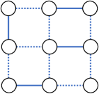
Figure 2. The $3\times 3$ grid topology; an example of link schedule subject to node-exclusive interference, which forms a matching, is shown in solid lines.

For both MW-UCB and MW with restart UCB (Stahlbuhk et al., 2019), we set the restart period to $\tau=T^{2/3}$. Sliding window size of MW-UCB is set to $d=2\lceil\tau^{\frac{2}{3}(1-\alpha)}\rceil+150$. We perform extensive testing on the $3\times 3$ grid network with node-exclusive wireless interference constraints (Bui et al., 2009), as depicted in Figure 2. To model the non-stationary service rates, for any time slot $t$ and link $e\in E$, we consider $\mu_{e}(t)$ evolving over time according to the Markov chain in Figure 3, whereby $\mu_{e}(t)$ would change its state (between $0.25$ and $0.75$) with probability $\delta_{t}$ which itself may vary over time. Then, given $\mu_{e}(t)$, the instantaneous service capacity $\theta_{e}(t)\sim Rayleigh\big{(}\sqrt{\frac{2}{\pi}}\mu_{e}(t)\big{)}$ is sampled from the Rayleigh distribution with the scale parameter that ensures $\mathbb{E}[\theta_{e}(t)]=\mu_{e}(t)$. We consider two settings of $\delta_{t}$, which governs the dynamics of the non-stationary service rates:

1. Time-invariant $\delta_{t}=\frac{0.5}{T^{1/2}}$: This corresponds to the uniformly changing dynamics and was considered in the literature (Stahlbuhk et al., 2019) for simulations.

2. Time-varying $\delta_{t}=\frac{0.5}{(t+1)^{1/2}}$: This non-stationary aperiodic setting captures more abruptly changing environments.

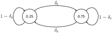
Figure 3. Markov chain for the time-varying mean service rate $\mu_{e}(t),\forall e\in E$. At time slot $t$ and for any edge $e$, given $\mu_{e}(t)\in\{0.25,0.75\}$, the instantaneous service capacity $\theta_{e}(t)$ follows Rayleigh distribution with mean $\mu_{e}(t)$.

Moreover, both of the above settings satisfy Assumption 1 in the sense that $\mathbb{E}[\gamma(t_{1},t_{2})]=O(|t_{2}-t_{1}|^{1/2})$ for any $0\leq t_{1}<t_{2}\leq T$ (see Appendix F for the proof). We thus use $\alpha=1/2$ in our simulations.

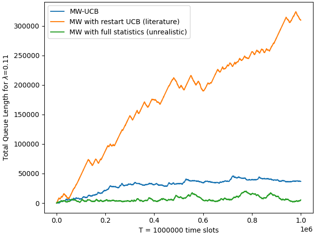
(a) Fixed arrival rate $\lambda=0.11$ strictly within the stability region.

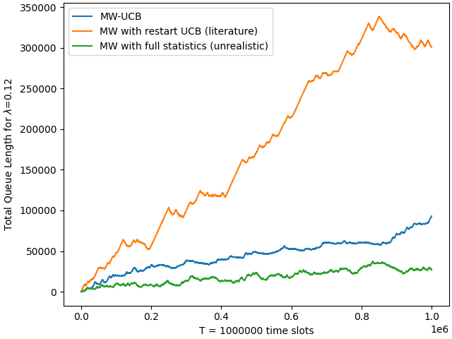
(b) Fixed arrival rate $\lambda=0.12$ strictly outside the stability region.

(c) Adaptive arrival rates $\bar{\lambda}(t)$ of highly loaded network.

Figure 4. Total queue length over time for time-invariant $\delta_{t}=\frac{0.5}{T^{1/2}}$.

5.1. Throughput-Optimality and Stability

We first consider fixed arrival rates where, at time slot $t$, every link receives Poisson arrivals with the same packet generation rate $\lambda=\lambda_{e}(t),\forall e\in E$. To demonstrate the stability properties of the algorithms, we investigate the evolution of the total queue backlog, i.e. $\sum_{e\in E}Q_{e}(t)$ at time $t$, for $\lambda=0.11$ and $0.12$, which respectively represent the regimes of moderately loaded and highly loaded network. We run the simulations for $T=10^{6}$ time slots and report the results for both settings of time-invariant $\delta_{t}$ and time-varying $\delta_{t}$ in Figure 4 and Figure 5, respectively.

Throughput-Optimality of MW-UCB: The results from Figure 4 and Figure 5 demonstrate that MW-UCB preserves the stability property of the idealized MW policy and thus supports the same stability region as achieved by the class of idealized policies with full statistics. In particular, the total queue backlogs of both algorithms remain stable for the moderate-load regime $\lambda=0.11$, and start to explode in the high-load regime $\lambda=0.12$.

Performance Evaluation of MW-UCB: In all experiments from Figure 4 and Figure 5, MW-UCB consistently outperforms MW with restart UCB. Whenever the arrival rate $\lambda$ is inside the stability region (Figure 4(a) and Figure 5(a)), MW-UCB can learn the channels’ statistics under non-stationarity and consequently stabilize the system. Additionally, for MW-UCB and idealized MW, we gradually increase $\lambda=0.03\to 0.22$ and report in Figure 6 the value of $\log\big{(}{\sum_{e\in E}Q_{e}(T)}/{T}\big{)}$ at $T=1.5\cdot 10^{6}$ to empirically measure the closeness of ${Q_{T}}/{T}$ to $0$ as well as its growth outside the stability region. The result suggests that MW-UCB preserves the pattern of idealized MW.

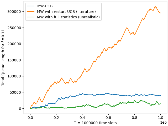
(a) Fixed arrival rate $\lambda=0.11$ strictly within the stability region.

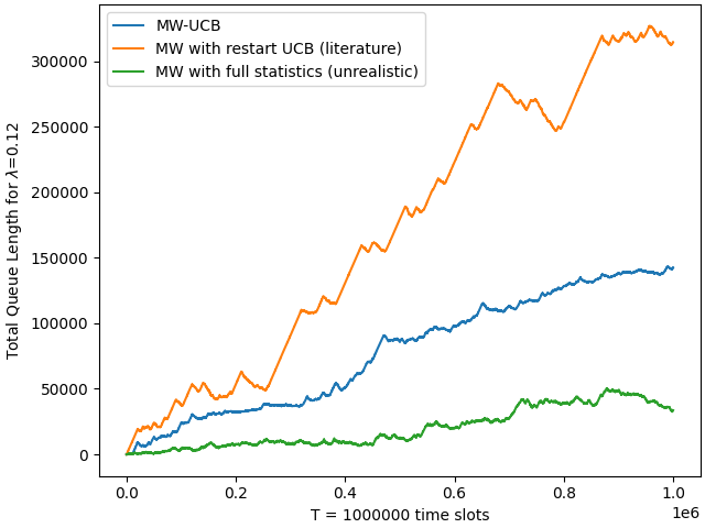
(b) Fixed arrival rate $\lambda=0.12$ strictly outside the stability region.

(c) Adaptive arrival rates $\bar{\lambda}(t)$ of highly loaded network.

Figure 5. Total queue length over time for time-varying $\delta_{t}=\frac{0.5}{(t+1)^{1/2}}$.

(a) Setting of time-invariant $\delta_{t}=\frac{0.5}{T^{1/2}}$.

(b) Setting of time-varying $\delta_{t}=\frac{0.5}{(t+1)^{1/2}}$.

Figure 6. Measuring $\log(Q_{T}/T)$ at $T=1.5\cdot 10^{6}$ for $\lambda=0.03\to 0.22$.

5.2. Time-Varying Arrival Rates

Next, we provide additional simulations for time-varying arrival rates $\boldsymbol{\lambda}(t)$. We let all links in any time slot $t$ to receive Poisson arrivals with the same packet generation rate $\bar{\lambda}(t)=\lambda_{e}(t),\forall e\in E$. Given the mean service rates $\boldsymbol{\mu}(t)$, an upper-bound on the maximum arrival rate supported by the network is given by:

(23) $$\bar{\lambda}(t)\leq\min_{v\in V}\frac{1}{\sum_{e\in\mathcal{A}(v)}\mu_{e}(t)^{-1}},$$

where $\mathcal{A}(v)$ is the set of links adjacent to node $v$. In our simulations, we set $\bar{\lambda}(t)$ to be exactly the right-hand side of (23) to model highly loaded network. We plot the total queue length over time, i.e. $\sum_{e\in E}Q_{e}(t)$ at time $t$, for both settings of time-invariant $\delta_{t}$ and time-varying $\delta_{t}$ respectively in Figure 4(c) and Figure 5(c). The results demonstrate that MW-UCB can well adapt to the time-varying arrival rates to achieve stability, and consistently improves over MW with restart UCB.

6. Conclusion

In this paper, we present MW-UCB as a novel joint learning and scheduling algorithm for non-stationary wireless network control under partial observability and non-stationary dynamics. Our algorithmic development is based on the Max-Weight policy for network control and sliding-window UCB for learning uncertain and time-varying channel statistics. We propose a new notion of stability for non-stationary networks and prove that the MW-UCB algorithm achieves a stability region that is arbitrarily close to the true stability region. Extensive simulations on both uniformly changing and abruptly changing dynamics confirm the throughput-optimality and the favorable performance of the algorithm. We believe that our analytical framework can be extended to study stability properties of algorithms for non-stationary network control under stringent requirements of emerging large-scale wireless networks.

Appendix

Appendix A Proof of Lemma 6

First, we prove that $\mathbf{\Lambda}_{s}(\beta_{1})\subseteq\mathbf{\Lambda}_{s}(\beta_{2})$ for any $0\leq\beta_{1}\leq\beta_{2}\leq 1$. Take any $\{\boldsymbol{\lambda}(t)\}_{t\geq 0}\in\mathbf{\Lambda}_{s}(\beta_{1})$. Then there exists some $\pi\in\Pi_{s}$ such that $Q_{T}^{\pi}=O\big{(}T^{\beta_{1}}\big{)}$. Since $\beta_{1}\leq\beta_{2}$, this implies $Q_{T}^{\pi}=O\big{(}T^{\beta_{2}}\big{)}$ and thus $\{\boldsymbol{\lambda}(t)\}_{t\geq 0}\in\mathbf{\Lambda}_{s}(\beta_{2})$. Therefore, we have $\mathbf{\Lambda}_{s}(\beta_{1})\subseteq\mathbf{\Lambda}_{s}(\beta_{2})$.

Second, we prove that $\mathbf{\Lambda}_{s}(\beta)\subseteq\mathbf{\Lambda}_{s}$ for any $\beta\in[0,1)$. Take any $\{\boldsymbol{\lambda}(t)\}_{t\geq 0}\in\mathbf{\Lambda}_{s}(\beta)$. Then there exists some $\pi\in\Pi_{s}$ such that $Q_{T}^{\pi}=O\big{(}T^{\beta}\big{)}$. Since $\beta<1$, this implies $Q_{T}^{\pi}=o\big{(}T\big{)}$ and thus $\{\boldsymbol{\lambda}(t)\}_{t\geq 0}\in\mathbf{\Lambda}_{s}$. Therefore, we have $\mathbf{\Lambda}_{s}(\beta)\subseteq\mathbf{\Lambda}_{s}$.

Finally, we prove that $\mathbf{\Lambda}_{s}\subseteq\mathbf{\Lambda}_{s}(1)$. Take any $\{\boldsymbol{\lambda}(t)\}_{t\geq 0}\in\mathbf{\Lambda}_{s}$. Then there exists some $\pi\in\Pi_{s}$ such that $Q_{T}^{\pi}=o\big{(}T\big{)}$, which implies $Q_{T}^{\pi}=O\big{(}T\big{)}$ and thus $\{\boldsymbol{\lambda}(t)\}_{t\geq 0}\in\mathbf{\Lambda}_{s}(1)$. Therefore, we have $\mathbf{\Lambda}_{s}\subseteq\mathbf{\Lambda}_{s}(1)$.

Appendix B Proof of Theorem 9

Since $\boldsymbol{\lambda}\in\bar{\mathbf{\Lambda}}_{s}$, by definition there exists some $\pi^{*}\in\Pi_{s}$ that satisfies:

(24) $$\lambda_{e}=\lim_{T\to\infty}\frac{1}{T}\sum_{t=0}^{T-1}a_{e}(t)\leq\lim_{T\to\infty}\frac{1}{T}\sum_{t=0}^{T-1}b^{\pi^{*}}_{e}(t),\forall e\in E.$$

Let $\mathbf{x}^{1},\mathbf{x}^{2},...,\mathbf{x}^{|\mathcal{M}|}$ be all the admissible link activations in $\mathcal{M}$. For any time slot $t>0$, we consider the empirical counter and distribution $\forall i\in[1,|\mathcal{M}|]$:

(25) $$n_{i}(t) =\sum_{s=0}^{t-1}\mathbbm{1}_{\{\mathbf{x}^{\pi^{*}}(s)=\mathbf{x}^{i}\}},$$

(26) $$p_{i}(t) =\frac{n_{i}(t)}{t},$$

where $n_{i}(t)$ and $p_{i}(t)$ respectively represent the number of times and the time fraction that the link activation vector $\mathbf{x}^{i}$ has been chosen by the policy $\pi^{*}$ by time $t$. Additionally, we consider $\forall i\in[1,|\mathcal{M}|]$:

(27) $$S_{i,e}(t)=\begin{cases}0,\text{ if $x^{i}_{e}=0$}\\ \frac{\sum_{s=0}^{t-1}\theta_{e}(s)\mathbbm{1}_{\{\mathbf{x}^{\pi^{*}}(s)=\mathbf{x}^{i}\}}}{n_{i}(t)},\text{ otherwise}\end{cases}.$$

Let $\mathbf{p}(t)=(p_{i}(t))_{i\in[1,|\mathcal{M}|]}$ be the vector of all such empirical distributions. Also note that $\sum_{i=1}^{|\mathcal{M}|}p_{i}(t)=1$ for any $t>0$. Since $\mathbf{p}(t)\in[0,1]^{|\mathcal{M}|}$, by the Bolzano–Weierstrass Theorem, there exists a convergent subsequence $\{\mathbf{p}(t_{k})\}_{k=1,2,...}$ where $\lim_{k\to\infty}t_{k}=\infty$. Define the limit of this convergent subsequence by:

(28) $$\mathbf{p}^{*}=\lim_{k\to\infty}\mathbf{p}(t_{k}).$$

Now, we note that for any $i\in[1,|\mathcal{M}|]$ such that $p^{*}_{i}>0$ (which also implies $\lim_{k\to\infty}n_{i}(t_{k})=\infty$), by SLLN, we have:

(29) $$\lim_{k\to\infty}S_{i,e}(t_{k})=\mathbbm{1}_{\{x^{i}_{e}=1\}}\mu_{e},\forall e\in E.$$

With the convention that $0/0=0$, we obtain from (24) that $\forall e\in E$:

$$\lambda_{e} \leq\lim_{k\to\infty}\frac{1}{t_{k}}\sum_{s=0}^{t_{k}-1}b^{\pi^{*}}_{e}(s)$$

$$=\lim_{k\to\infty}\sum_{i=1}^{|\mathcal{M}|}p_{i}(t_{k})\cdot S_{i,e}(t_{k})$$

(30) $$\overset{\eqref{equivalence_proof5}+\eqref{equivalence_proof6}}{=}\mu_{e}\sum_{i=1}^{|\mathcal{M}|}p^{*}_{i}\cdot\mathbbm{1}_{\{x^{i}_{e}=1\}}$$

Consider a stationary randomized policy $\pi_{r}$ that at any time $t$ activates the link schedule $\mathbf{x}^{\pi_{r}}(t)=\mathbf{x}^{i}$ with probability $p^{*}_{i}$. Next, we consider the Max-Weight (MW) policy with the full knowledge of the statistics (i.e. MW is in $\Pi_{s}$) that at any time slot $t$, schedules the link according to:

(31) $$\mathbf{x}^{\textsc{MW}}(t)=\operatorname*{\arg\!\max}_{\mathbf{x}\in\mathcal{M}}\big{\{}\sum_{e\in E}Q^{\textsc{MW}}_{e}(t)\mu_{e}x_{e}\big{\}},$$

and proceeds to show that $Q_{T}^{\textsc{MW}}=O\big{(}T^{\frac{1}{2}}\big{)}$. For brevity, we use $\pi_{M}$ to denote the MW policy. Under the MW policy, we consider the quadratic Lyapunov function of the queue lengths $\mathbf{Q}^{\pi_{M}}(t)$ as:

(32) $$\Phi^{\pi_{M}}(\mathbf{Q}^{\pi_{M}}(t))=\mathbf{Q}^{\pi_{M}}(t)^{T}\mathbf{Q}^{\pi_{M}}(t)=\sum_{e\in E}Q^{\pi_{M}}_{e}(t)^{2}.$$

We consider the $1$-step Lyapunov drift conditioned on the queue length as follows:

(33) $$\Delta^{\pi_{M}}(t)=\mathbb{E}\big{[}\Phi^{\pi_{M}}(\mathbf{Q}^{\pi_{M}}(t+1))-\Phi^{\pi_{M}}(\mathbf{Q}^{\pi_{M}}(t))\big{|}\mathbf{Q}^{\pi_{M}}(t)\big{]}.$$

From the queue process (2), we first obtain that $\forall e\in E,t\geq 0$:

$$Q^{\pi_{M}}_{e}(t+1)^{2} \leq\big{(}Q^{\pi_{M}}_{e}(t)+{a}_{e}(t)-b^{\pi_{M}}_{e}(t)\big{)}^{2}$$

$$=Q^{\pi_{M}}_{e}(t)^{2}+({a}_{e}(t)-b^{\pi_{M}}_{e}(t))^{2}$$

$$\quad+2Q^{\pi_{M}}_{e}(t)({a}_{e}(t)-b^{\pi_{M}}_{e}(t))$$

$$\leq Q^{\pi_{M}}_{e}(t)^{2}+(A_{max}+\mu_{max})^{2}$$

$$\quad+2Q^{\pi_{M}}_{e}(\tau_{j})({a}_{e}(t)-b^{\pi_{M}}_{e}(t)),$$

where in the last line we use $0\leq a_{e}(t)\leq A_{max}$, $0\leq b^{\pi_{M}}_{e}(t)\leq\theta_{e}(t)\leq\mu_{max}$. Summing the above over all $e\in E$ and taking the expectation conditioned on $\mathbf{Q}^{\pi_{M}}(t)$, we obtain that:

$$\Delta^{\pi_{M}}(t) \leq|E|(A_{max}+\mu_{max})^{2}+2\sum_{e\in E}Q^{\pi_{M}}_{e}(t)\lambda_{e}(t)$$

$$\quad-2\sum_{e\in E}Q^{\pi_{M}}_{e}(t)\mu_{e}\mathbb{E}\big{[}x^{\pi_{M}}_{e}(t)\big{|}\mathbf{Q}^{\pi_{M}}(t)\big{]}$$

$$\overset{\eqref{MW_proof1}}{\leq}|E|(A_{max}+\mu_{max})^{2}+2\sum_{e\in E}Q^{\pi_{M}}_{e}(t)\lambda_{e}(t)$$

$$\quad-2\sum_{e\in E}Q^{\pi_{M}}_{e}(t)\mu_{e}\mathbb{E}\big{[}x^{\pi_{r}}_{e}(t)\big{|}\mathbf{Q}^{\pi_{M}}(t)\big{]}$$

$$=|E|(A_{max}+\mu_{max})^{2}+2\sum_{e\in E}Q^{\pi_{M}}_{e}(t)\lambda_{e}(t)$$

$$\quad-2\sum_{e\in E}Q^{\pi_{M}}_{e}(t)\mu_{e}\sum_{i=1}^{|\mathcal{M}|}p^{*}_{i}\cdot\mathbbm{1}_{\{x^{i}_{e}=1\}}$$

$$\overset{\eqref{equivalence_proof7}}{\leq}|E|(A_{max}+\mu_{max})^{2}.$$

Taking expectation of both sides with respect to $\mathbf{Q}^{\pi_{M}}(t)$, we have:

$$\mathbb{E}\big{[}\Phi^{\pi_{M}}(\mathbf{Q}^{\pi_{M}}(t+1))\big{]}-\mathbb{E}\big{[}\Phi^{\pi_{M}}(\mathbf{Q}^{\pi_{M}}(t))\big{]}\leq|E|(A_{max}+\mu_{max})^{2}.$$

Telescoping over $t=0\to T-1$ and noting that $\Phi^{\pi_{M}}(\mathbf{Q}^{\pi_{M}}(0))=0$, we get:

(34) $$\mathbb{E}\big{[}\Phi^{\pi_{M}}(\mathbf{Q}^{\pi_{M}}(T))\big{]}\leq T|E|(A_{max}+\mu_{max})^{2}.$$

Following the same argument as the proof of Lemma 5, we can similarly obtain that:

$$Q_{T}^{\textsc{MW}}=\mathbb{E}\big{[}\sum_{e\in E}Q^{\pi_{M}}_{e}(T)\big{]} \leq\sqrt{|E|\cdot\mathbb{E}\big{[}\Phi^{\pi_{M}}(\mathbf{Q}^{\pi_{M}}(T))\big{]}}$$

$$\overset{\eqref{equivalence_proof8}}{\leq}T^{\frac{1}{2}}|E|(A_{max}+\mu_{max}),$$

which implies $Q_{T}^{\textsc{MW}}=O\big{(}T^{\frac{1}{2}}\big{)}$. Since $\pi_{M}\in\Pi_{s}$, we thus have $\boldsymbol{\lambda}\in\mathbf{\Lambda}_{s}(\frac{1}{2})$. Since by our Definition 8, a throughput-optimal policy $\pi$, given $\beta\in[0,1)$, achieves the stability region $\mathbf{\Lambda}_{s}(\beta)$, the network is mean rate stable under $\pi$ for any $\boldsymbol{\lambda}\in\bar{\mathbf{\Lambda}}_{s}$.

Appendix C Proof of Lemma 4

Since $\{\boldsymbol{\lambda}(t)\}_{t\geq 0}\in\mathbf{\Lambda}_{s}(\beta)$, by definition there exists some policy $\pi^{*}\in\Pi_{s}$ such that:

$$Q_{T}^{\pi^{*}}=O(T^{\beta}).$$

For any $\tau_{j}$, we consider $\forall e\in E$:

(35) $$r_{e}(\tau_{j})=\begin{cases}0,\text{ if }\sum_{t=\tau_{j}}^{\tau_{j+1}-1}\lambda_{e}(t)=0\\ \bigg{(}\frac{(1-\varepsilon)(\sum_{t=\tau_{j}}^{\tau_{j+1}-1}\lambda_{e}(t)-\mathbb{E}[Q_{e}^{\pi^{*}}(\tau_{j+1})])}{\sum_{t=\tau_{j}}^{\tau_{j+1}-1}\lambda_{e}(t)}\bigg{)}^{+},\text{ otherwise }\end{cases}$$

and sheds the traffics such that for any $t\in[\tau_{j},\tau_{j+1})$,

(36) $$\tilde{a}_{e}(t)=r_{e}(\tau_{j})a_{e}(t),\forall e\in E.$$

We now proceed to show that this shedding scheme guarantees $\{\tilde{\boldsymbol{\lambda}}(t)\}_{t\geq 0}\in\mathcal{C}(\tau,\varepsilon)$ and (18).

From the queue dynamics (2), we have $\forall e\in E$:

$$Q_{e}^{\pi^{*}}(\tau_{j+1}) =\big{(}Q^{\pi^{*}}_{e}(\tau_{j+1}-1)+a_{e}(\tau_{j+1}-1)-b^{\pi^{*}}_{e}(\tau_{j+1}-1)\big{)}^{+}$$

$$\geq Q^{\pi^{*}}_{e}(\tau_{j+1}-1)+a_{e}(\tau_{j+1}-1)-b^{\pi^{*}}_{e}(\tau_{j+1}-1).$$

By repeating the above argument, we get $\forall e\in E$:

$$Q_{e}^{\pi^{*}}(\tau_{j+1}) \geq Q^{\pi^{*}}_{e}(\tau_{j})+\sum_{t=\tau_{j}}^{\tau_{j+1}-1}a_{e}(t)-\sum_{t=\tau_{j}}^{\tau_{j+1}-1}b^{\pi^{*}}_{e}(t)$$

$$\geq\sum_{t=\tau_{j}}^{\tau_{j+1}-1}a_{e}(t)-\sum_{t=\tau_{j}}^{\tau_{j+1}-1}b^{\pi^{*}}_{e}(t).$$

Taking expectation of the above, we obtain that:

$$\sum_{t=\tau_{j}}^{\tau_{j+1}-1}\lambda_{e}(t)-\mathbb{E}[Q_{e}^{\pi^{*}}(\tau_{j+1})]\leq\sum_{t=\tau_{j}}^{\tau_{j+1}-1}\mathbb{E}[b^{\pi^{*}}_{e}(t)],\quad\forall e\in E.$$

(37) $$\therefore\bigg{(}\sum_{t=\tau_{j}}^{\tau_{j+1}-1}\lambda_{e}(t)-\mathbb{E}[Q_{e}^{\pi^{*}}(\tau_{j+1})]\bigg{)}^{+}\leq\sum_{t=\tau_{j}}^{\tau_{j+1}-1}\mathbb{E}[b^{\pi^{*}}_{e}(t)],\quad\forall e\in E.$$

Taking expectation of (36) and summing over $t=\tau_{j}\to\tau_{j+1}-1$, we obtain in view of (35) and (37) that $\forall e\in E$:

$$\sum_{t=\tau_{j}}^{\tau_{j+1}-1}\tilde{\lambda}_{e}(t)\overset{\eqref{shedding_inter2}}{=}r_{e}(\tau_{j})\big{(}\sum_{t=\tau_{j}}^{\tau_{j+1}-1}\lambda_{e}(t)\big{)}\overset{\eqref{shedding_inter1}+\eqref{shedding_inter3}}{\leq}(1-\varepsilon)\sum_{t=\tau_{j}}^{\tau_{j+1}-1}\mathbb{E}[b^{\pi^{*}}_{e}(t)],$$

which verifies $\{\tilde{\boldsymbol{\lambda}}(t)\}_{t\geq 0}\in\mathcal{C}(\tau,\varepsilon)$.

To prove (18), we note that from (17), $\mathbb{E}[X_{T}]=\sum_{t=0}^{T-1}\sum_{e\in E}\lambda_{e}(t)-\sum_{t=0}^{T-1}\sum_{e\in E}\tilde{\lambda}_{e}(t)$, and first proceeds to upper-bound $\sum_{t=\tau_{j}}^{\tau_{j+1}-1}\lambda_{e}(t)-\sum_{t=\tau_{j}}^{\tau_{j+1}-1}\tilde{\lambda}_{e}(t)$ by considering two cases as follows.
Case 1: $\sum_{t=\tau_{j}}^{\tau_{j+1}-1}\lambda_{e}(t)\leq\mathbb{E}[Q_{e}^{\pi^{*}}(\tau_{j+1})]$. From (35), we have $r_{e}(\tau_{j})=0$ and thus (from (36)) $\tilde{\lambda}_{e}(t)=\mathbb{E}[\tilde{a}_{e}(t)]=0$. Then we obtain that:

$$\sum_{t=\tau_{j}}^{\tau_{j+1}-1}\lambda_{e}(t)-\sum_{t=\tau_{j}}^{\tau_{j+1}-1}\tilde{\lambda}_{e}(t)=\sum_{t=\tau_{j}}^{\tau_{j+1}-1}\lambda_{e}(t)\leq\mathbb{E}[Q_{e}^{\pi^{*}}(\tau_{j+1})].$$

Case 2: $\sum_{t=\tau_{j}}^{\tau_{j+1}-1}\lambda_{e}(t)>\mathbb{E}[Q_{e}^{\pi^{*}}(\tau_{j+1})]\geq 0$. We have:

$$\sum_{t=\tau_{j}}^{\tau_{j+1}-1}\lambda_{e}(t)-\sum_{t=\tau_{j}}^{\tau_{j+1}-1}\tilde{\lambda}_{e}(t) \overset{\eqref{shedding_inter2}}{=}(1-r_{e}(\tau_{j}))\big{(}\sum_{t=\tau_{j}}^{\tau_{j+1}-1}\lambda_{e}(t)\big{)}$$

$$\overset{\eqref{shedding_inter1}}{=}\varepsilon\big{(}\sum_{t=\tau_{j}}^{\tau_{j+1}-1}\lambda_{e}(t)\big{)}+(1-\varepsilon)\mathbb{E}[Q_{e}^{\pi^{*}}(\tau_{j+1})]$$

$$\leq\varepsilon\tau A_{max}+\mathbb{E}[Q_{e}^{\pi^{*}}(\tau_{j+1})]$$

Thus, in any case, we have:

$$\sum_{t=\tau_{j}}^{\tau_{j+1}-1}\lambda_{e}(t)-\sum_{t=\tau_{j}}^{\tau_{j+1}-1}\tilde{\lambda}_{e}(t)\leq\varepsilon\tau A_{max}+\mathbb{E}[Q_{e}^{\pi^{*}}(\tau_{j+1})].$$

Summing the above over all $e\in E$ and $j=0\to K-1$, we obtain:

$$\mathbb{E}[X_{\tau_{K}}] =\sum_{t=0}^{\tau_{K}-1}\sum_{e\in E}\lambda_{e}(t)-\sum_{t=0}^{\tau_{K}-1}\sum_{e\in E}\tilde{\lambda}_{e}(t)$$

$$\leq\varepsilon\tau KA_{max}+\sum_{j=0}^{K-1}\mathbb{E}[\sum_{e\in E}Q_{e}^{\pi^{*}}(\tau_{j+1})]$$

$$=\varepsilon\tau KA_{max}+\sum_{j=1}^{K}Q^{\pi^{*}}_{\tau_{j}}$$

$$=O\big{(}\varepsilon\tau K+\sum_{j=1}^{K}\tau_{j}^{\beta}\big{)}$$

$$=O\big{(}\varepsilon\tau K+\tau_{K}^{\beta}+\sum_{j=1}^{K-1}\frac{1}{\tau}\int_{\tau_{j}}^{\tau_{j+1}}x^{\beta}dx\big{)}$$

$$=O\big{(}\varepsilon\tau K+\tau_{K}^{\beta}+\frac{1}{\tau}\int_{\tau_{1}}^{\tau_{K}}x^{\beta}dx\big{)}$$

$$=O\big{(}\varepsilon\tau K+\tau_{K}^{\beta}+\frac{1}{\tau}\int_{\tau_{1}}^{\tau_{K}}x^{\beta}dx\big{)}$$

$$=O\big{(}\varepsilon\tau_{K}+\tau_{K}^{\beta}+\frac{\tau_{K}^{\beta+1}}{\tau}\big{)}$$

(38) $$=O\big{(}T^{\beta+1}\tau^{-1}+\varepsilon T\big{)}.$$

Finally, we have:

$$\mathbb{E}[X_{T}] =\mathbb{E}[X_{\tau_{K}}]+\sum_{t=\tau_{K}}^{T-1}\sum_{e\in E}\lambda_{e}(t)-\sum_{t=\tau_{K}}^{T-1}\sum_{e\in E}\tilde{\lambda}_{e}(t)$$

$$\leq\mathbb{E}[X_{\tau_{K}}]+\tau|E|A_{max}$$

$$\overset{\eqref{shedding_inter4}}{=}O\big{(}T^{\beta+1}\tau^{-1}+\varepsilon T+\tau\big{)}.$$

Appendix D Guarantees of the imaginary system’s queue process $\{\widetilde{\mathbf{Q}}(t)\}_{t\geq 0}$

Recall from Section 4.3 that:

• When MW-UCB is applied to the original system, it produces the sequence of decisions $\{\mathbf{x}^{\textsc{MW-UCB}}(t)\}_{t\geq 0}$ and thus effective service rate $\{\mathbf{b}^{\textsc{MW-UCB}}(t)\}_{t\geq 0}$. The queueing dynamics of the original system evolves as $\{\mathbf{Q}^{\textsc{MW-UCB}}(t)\}_{t\geq 0}$ via:

  $$Q^{\textsc{MW-UCB}}_{e}(t+1)=\big{(}Q^{\textsc{MW-UCB}}_{e}(t)+a_{e}(t)-b^{\textsc{MW-UCB}}_{e}(t)\big{)}^{+},\forall e\in E.$$

• The ”imaginary” queue lengths $\widetilde{\mathbf{Q}}(t)$ evolve as the sequence of decisions $\{\mathbf{x}^{\textsc{MW-UCB}}(t)\}_{t\geq 0}$ is applied to the imaginary system, i.e.

  $$\widetilde{Q}_{e}(t+1)=\big{(}\widetilde{Q}_{e}(t)+\tilde{a}_{e}(t)-b^{\textsc{MW-UCB}}_{e}(t)\big{)}^{+},\forall e\in E.$$

In the proofs of this Appendix D, we refer to $\{\mathbf{x}^{\textsc{MW-UCB}}(t)\}_{t\geq 0}$, $\{\mathbf{b}^{\textsc{MW-UCB}}(t)\}_{t\geq 0}$ and $\{\mathbf{Q}^{\textsc{MW-UCB}}(t)\}_{t\geq 0}$ respectively as $\{\mathbf{x}(t)\}_{t\geq 0}$, $\{\mathbf{b}(t)\}_{t\geq 0}$ and $\{\mathbf{Q}(t)\}_{t\geq 0}$ for brevity. Consequently, the queueing dynamics of the original system and imaginary system can be respectively expressed as:

(39) $$Q_{e}(t+1)=\big{(}Q_{e}(t)+a_{e}(t)-b_{e}(t)\big{)}^{+},\forall e\in E$$

(40) $$\widetilde{Q}_{e}(t+1)=\big{(}\widetilde{Q}_{e}(t)+\tilde{a}_{e}(t)-b_{e}(t)\big{)}^{+},\forall e\in E.$$

D.1. Proof of Lemma 5

From Lemma 1, we have $\forall e\in E$:

$$Q_{e}(T)\leq\widetilde{Q}_{e}(T)+\sum_{q=0}^{T-1}(a_{e}(q)-\tilde{a}_{e}(q))$$

Summing up the above over all $e\in E$ and taking expectation, we conclude that:

$$\mathbb{E}[\sum_{e\in E}Q_{e}(T)]\leq\mathbb{E}[\sum_{q=0}^{T-1}(a_{e}(q)-\tilde{a}_{e}(q))]+\mathbb{E}\big{[}\sum_{e\in E}\widetilde{Q}_{e}(T)\big{]}$$

$$\therefore Q_{T}^{\textsc{MW-UCB}}\leq\mathbb{E}[X_{T}]+\mathbb{E}\big{[}\sum_{e\in E}\widetilde{Q}_{e}(T)\big{]},$$

where the last line follows from the definitions of $Q_{T}$ and $X_{T}$.

D.2. Proof of Lemma 6

Since $\{\tilde{\boldsymbol{\lambda}}(t)\}_{t\geq 0}\in\mathcal{C}(\tau,\varepsilon)$, by definition there exists some $\pi_{0}\in\Pi_{s}$ such that for any $\tau_{j}\in\{\tau_{0},\tau_{1},...,\tau_{K-1}\}$:

(41) $$\sum_{t=\tau_{j}}^{\tau_{j+1}-1}\tilde{\lambda}_{e}(t)\leq(1-\varepsilon)\sum_{t=\tau_{j}}^{\tau_{j+1}-1}\mathbb{E}[b^{\pi_{0}}_{e}(t)],\text{ }\forall e\in E.$$

We consider the quadratic Lyapunov function of the queue lengths $\widetilde{\mathbf{Q}}(t)$ of the imaginary system under MW-UCB as:

(42) $$\Phi(\widetilde{\mathbf{Q}}(t))=\widetilde{\mathbf{Q}}(t)^{T}\widetilde{\mathbf{Q}}(t)=\sum_{e\in E}\widetilde{Q}_{e}(t)^{2}.$$

We consider the $\tau$-step Lyapunov drift of $\Phi(.)$ conditioned on the queue lengths of both the original system and the imaginary system as follows:

(43) $$\Delta(\tau_{j})=\mathbb{E}\big{[}\Phi(\widetilde{\mathbf{Q}}(\tau_{j+1}))-\Phi(\widetilde{\mathbf{Q}}(\tau_{j}))\big{|}\widetilde{\mathbf{Q}}(\tau_{j}),\mathbf{Q}(\tau_{j})\big{]},$$

where we recall that $\tau_{j}=j\tau$. From Lemma 2 (in Appendix D.3), the drift can be upper-bounded by:

$$\Delta(\tau_{j}) \leq B_{1}\tau(\tau+1)+2\sum_{t=\tau_{j}}^{\tau_{j+1}-1}\widetilde{\mathbf{Q}}(\tau_{j})^{T}\tilde{\boldsymbol{\lambda}}(t)$$

(44) $$\quad-2\sum_{t=\tau_{j}}^{\tau_{j+1}-1}\mathbb{E}[\widetilde{\mathbf{Q}}(\tau_{j})^{T}\mathbf{b}(t)\big{|}\widetilde{\mathbf{Q}}(\tau_{j}),\mathbf{Q}(\tau_{j})],$$

where $B_{1}=\frac{1}{2}|E|(A_{max}+\mu_{max})^{2}$. Now, we consider the normalized queue lengths of both the original and imaginary systems as:

(45) $$\tilde{w}_{e}(\tau_{j})=\frac{\widetilde{Q}_{e}(\tau_{j})}{\|\widetilde{\mathbf{Q}}(\tau_{j})\|_{\infty}},\forall e\in E,$$

(46) $$w_{e}(\tau_{j})=\frac{Q_{e}(\tau_{j})}{\|\mathbf{Q}(\tau_{j})\|_{\infty}},\forall e\in E,$$

with the convention that $0/0=0$. Note that (46) is the same weight updating rule as Line 1 of MW-UCB (Algorithm 1). Then we consider the following two regrets which respectively use (45) and (46) in their weight instantiations:

$$\bar{\mathcal{R}}(\tau_{j}) =\sum_{t=\tau_{j}}^{\tau_{j+1}-1}\max_{\mathbf{x}^{\prime}\in\mathcal{M}}\mathbb{E}\big{[}\sum_{e\in E}\tilde{w}_{e}(\tau_{j})x^{\prime}_{e}\theta_{e}(t)\big{|}\widetilde{\mathbf{Q}}(\tau_{j}),\mathbf{Q}(\tau_{j})\big{]}$$

(47) $$\quad-\sum_{t=\tau_{j}}^{\tau_{j+1}-1}\mathbb{E}\big{[}\sum_{e\in E}\tilde{w}_{e}(\tau_{j})x_{e}(t)\theta_{e}(t)\big{|}\widetilde{\mathbf{Q}}(\tau_{j}),\mathbf{Q}(\tau_{j})\big{]}$$

$$=\frac{1}{\|\widetilde{\mathbf{Q}}(\tau_{j})\|_{\infty}}\sum_{t=\tau_{j}}^{\tau_{j+1}-1}\max_{\mathbf{x}^{\prime}\in\mathcal{M}}\mathbb{E}\big{[}\sum_{e\in E}\widetilde{Q}_{e}(\tau_{j})x^{\prime}_{e}\theta_{e}(t)\big{|}\widetilde{\mathbf{Q}}(\tau_{j}),\mathbf{Q}(\tau_{j})\big{]}$$

(48) $$\quad-\frac{1}{\|\widetilde{\mathbf{Q}}(\tau_{j})\|_{\infty}}\sum_{t=\tau_{j}}^{\tau_{j+1}-1}\mathbb{E}\big{[}\widetilde{\mathbf{Q}}(\tau_{j})^{T}\mathbf{b}(t)\big{|}\widetilde{\mathbf{Q}}(\tau_{j}),\mathbf{Q}(\tau_{j})\big{]},$$

and (recalling from (16)),

$$\mathcal{R}(\tau_{j}) =\sum_{t=\tau_{j}}^{\tau_{j+1}-1}\max_{\mathbf{x}^{\prime}\in\mathcal{M}}\mathbb{E}\big{[}\sum_{e\in E}w_{e}(\tau_{j})x^{\prime}_{e}\theta_{e}(t)\big{|}\widetilde{\mathbf{Q}}(\tau_{j}),\mathbf{Q}(\tau_{j})\big{]}$$

(49) $$\quad-\sum_{t=\tau_{j}}^{\tau_{j+1}-1}\mathbb{E}\big{[}\sum_{e\in E}w_{e}(\tau_{j})x_{e}(t)\theta_{e}(t)\big{|}\widetilde{\mathbf{Q}}(\tau_{j}),\mathbf{Q}(\tau_{j})\big{]}$$

$$=\frac{1}{\|\mathbf{Q}(\tau_{j})\|_{\infty}}\sum_{t=\tau_{j}}^{\tau_{j+1}-1}\max_{\mathbf{x}^{\prime}\in\mathcal{M}}\mathbb{E}\big{[}\sum_{e\in E}Q_{e}(\tau_{j})x^{\prime}_{e}\theta_{e}(t)\big{|}\widetilde{\mathbf{Q}}(\tau_{j}),\mathbf{Q}(\tau_{j})\big{]}$$

(50) $$\quad-\frac{1}{\|\mathbf{Q}(\tau_{j})\|_{\infty}}\sum_{t=\tau_{j}}^{\tau_{j+1}-1}\mathbb{E}\big{[}\mathbf{Q}(\tau_{j})^{T}\mathbf{b}(t)\big{|}\widetilde{\mathbf{Q}}(\tau_{j}),\mathbf{Q}(\tau_{j})\big{]}.$$

From Lemma 3 (in Appendix D.3), we further relate (44) to the regret $\bar{\mathcal{R}}(\tau_{j})$ as follows:

$$\sum_{t=\tau_{j}}^{\tau_{j+1}-1}\mathbb{E}\big{[}\widetilde{\mathbf{Q}}(\tau_{j})^{T}\mathbf{b}(t)\big{|}\widetilde{\mathbf{Q}}(\tau_{j}),\mathbf{Q}(\tau_{j})\big{]}$$

$$\geq(1-\varepsilon)\sum_{t=\tau_{j}}^{\tau_{j+1}-1}\mathbb{E}\big{[}\widetilde{\mathbf{Q}}(\tau_{j})^{T}\mathbf{b}^{\pi_{0}}(t)\big{|}\widetilde{\mathbf{Q}}(\tau_{j}),\mathbf{Q}(\tau_{j})\big{]}$$

$$\quad+\varepsilon\tau\|\widetilde{\mathbf{Q}}(\tau_{j})\|_{\infty}\mu_{min}-\|\widetilde{\mathbf{Q}}(\tau_{j})\|_{\infty}\bar{\mathcal{R}}(\tau_{j})$$

$$=\sum_{e\in E}\widetilde{Q}_{e}(\tau_{j})\big{[}(1-\varepsilon)\sum_{t=\tau_{j}}^{\tau_{j+1}-1}\mathbb{E}[b_{e}^{\pi_{0}}(t)]\big{]}$$

$$\quad+\varepsilon\tau\|\widetilde{\mathbf{Q}}(\tau_{j})\|_{\infty}\mu_{min}-\|\widetilde{\mathbf{Q}}(\tau_{j})\|_{\infty}\bar{\mathcal{R}}(\tau_{j})$$

$$\overset{\eqref{window_stationary1}}{\geq}\sum_{e\in E}\widetilde{Q}_{e}(\tau_{j})\big{[}\sum_{t=\tau_{j}}^{\tau_{j+1}-1}\tilde{\lambda}_{e}(t)\big{]}$$

(51) $$\quad+\varepsilon\tau\|\widetilde{\mathbf{Q}}(\tau_{j})\|_{\infty}\mu_{min}-\|\widetilde{\mathbf{Q}}(\tau_{j})\|_{\infty}\bar{\mathcal{R}}(\tau_{j})$$

(52) $$=\sum_{t=\tau_{j}}^{\tau_{j+1}-1}\widetilde{\mathbf{Q}}(\tau_{j})^{T}\tilde{\boldsymbol{\lambda}}(t)+\varepsilon\tau\|\widetilde{\mathbf{Q}}(\tau_{j})\|_{\infty}\mu_{min}-\|\widetilde{\mathbf{Q}}(\tau_{j})\|_{\infty}\bar{\mathcal{R}}(\tau_{j})$$

where for (51) we recall that $\pi_{0}\in\Pi_{s}$ is the idealized policy that satisfies (41). Combining (52) and (44), we have:

(53) $$\Delta(\tau_{j}) \leq B_{1}\tau(\tau+1)-2\varepsilon\tau\|\widetilde{\mathbf{Q}}(\tau_{j})\|_{\infty}\mu_{min}+2\|\widetilde{\mathbf{Q}}(\tau_{j})\|_{\infty}\bar{\mathcal{R}}(\tau_{j}).$$

Now, we have from Lemma 4 (in Appendix D.3) that:

(54) $$\|\widetilde{\mathbf{Q}}(\tau_{j})\|_{\infty}\bar{\mathcal{R}}(\tau_{j})\leq\|\mathbf{Q}(\tau_{j})\|_{\infty}\mathcal{R}(\tau_{j})+\tau\mu_{max}\mathbb{E}[X_{\tau_{j}}].$$

and from Lemma 1 (in Appendix D.3) that:

(55) $$\mathbb{E}\big{[}\|\widetilde{\mathbf{Q}}(\tau_{j})\|_{\infty}\big{|}\widetilde{\mathbf{Q}}(\tau_{j}),\mathbf{Q}(\tau_{j})\big{]}\geq\mathbb{E}\big{[}\|\mathbf{Q}(\tau_{j})\|_{\infty}\big{|}\widetilde{\mathbf{Q}}(\tau_{j}),\mathbf{Q}(\tau_{j})\big{]}-\mathbb{E}[X_{\tau_{j}}]$$

Plugging (54) and (55) into (53), we obtain that:

$$\Delta(\tau_{j}) \leq B_{1}\tau(\tau+1)+2(\mu_{max}+\varepsilon\mu_{min})\tau\mathbb{E}[X_{\tau_{j}}]$$

(56) $$\quad-2\varepsilon\tau\|\mathbf{Q}(\tau_{j})\|_{\infty}\mu_{min}+2\|\mathbf{Q}(\tau_{j})\|_{\infty}\mathcal{R}(\tau_{j}).$$

Recall from Section 4.2 that MW-UCB, during every time frame $[\tau_{j},\tau_{j+1})$, fixes the queue length in the original system to $\mathbf{Q}(\tau_{j})$ (and thus the normalized weights $\{w_{e}(\tau_{j})\}_{e\in E}$), and adopts the CUCB-SW algorithm for scheduling while learning the non-stationary mean service rate. Thus, the regret $\mathcal{R}(\tau_{j})$ as in (49) serves to capture the learning efficiency of CUCB-SW with theoretical guarantee in (Chen et al., 2020). To this end, the regret bound under our choice of parameter $d=\tau^{\frac{2}{3}(1-\alpha)}$ is given by Lemma 1 (in Appendix D.3) as follows:

(57) $$\mathcal{R}(\tau_{j})\leq c_{0}\log(\tau)\tau^{\frac{1}{3}(\alpha+2)},$$

for some universal constant $c_{0}>0$ that can be explicitly determined. Substituting (57) into (56) and defining $c_{1}=\frac{c_{0}}{\mu_{min}}$, we have:

$$\Delta(\tau_{j}) \leq B_{1}\tau(\tau+1)+2(\mu_{max}+\varepsilon\mu_{min})\tau\mathbb{E}[X_{\tau_{j}}]$$

(58) $$\quad-2\tau\|\mathbf{Q}(\tau_{j})\|_{\infty}\mu_{min}\big{(}\varepsilon-c_{1}\log(\tau)\tau^{\frac{1}{3}(\alpha-1)}\big{)}.$$

Now, if $\varepsilon\geq c_{1}\log(\tau)\tau^{\frac{1}{3}(\alpha-1)}$, we obtain from (58) that:

$$\Delta(\tau_{j}) \leq B_{1}\tau(\tau+1)+2(\mu_{max}+\varepsilon\mu_{min})\tau\mathbb{E}[X_{\tau_{j}}].$$

Recall from (43) that $\Delta(\tau_{j})=\mathbb{E}\big{[}\Phi(\widetilde{\mathbf{Q}}(\tau_{j+1}))-\Phi(\widetilde{\mathbf{Q}}(\tau_{j}))\big{|}\widetilde{\mathbf{Q}}(\tau_{j}),\mathbf{Q}(\tau_{j})\big{]}$. Taking expectation on both sides of the above with respect to $\widetilde{\mathbf{Q}}(\tau_{j})$ and $\mathbf{Q}(\tau_{j})$, we get:

$$\mathbb{E}\big{[}\Phi(\widetilde{\mathbf{Q}}(\tau_{j+1}))\big{]}-\mathbb{E}\big{[}\Phi(\widetilde{\mathbf{Q}}(\tau_{j}))\big{]}$$

$$\leq B_{1}\tau(\tau+1)+2(\mu_{max}+\varepsilon\mu_{min})\tau\mathbb{E}[X_{\tau_{j}}].$$

Summing up the above for $j=0,1,...,K-1$ and noting that $\Phi(\widetilde{\mathbf{Q}}(\tau_{0}))=\Phi(\widetilde{\mathbf{Q}}(0))=0$, we obtain that:

$$\mathbb{E}\big{[}\Phi(\widetilde{\mathbf{Q}}(\tau_{K}))\big{]} \leq B_{1}\tau(\tau+1)K+2(\mu_{max}+\varepsilon\mu_{min})\tau\sum_{j=0}^{K-1}\mathbb{E}[X_{\tau_{j}}]$$

$$\overset{\eqref{shedding_cost}}{=}O\big{(}\tau^{2}K+\tau\sum_{j=0}^{K-1}(\tau_{j}^{\beta+1}\tau^{-1}+\varepsilon\tau_{j})\big{)}$$

$$=O\big{(}\tau^{2}K+\tau^{\beta+1}\sum_{j=0}^{K-1}j^{\beta+1}+\varepsilon\tau^{2}\sum_{j=0}^{K-1}j\big{)}$$

$$=O\big{(}\tau^{2}K+\tau^{\beta+1}\int_{0}^{K-1}x^{\beta+1}dx+\varepsilon\tau^{2}\sum_{j=0}^{K-1}j\big{)}$$

$$=O\big{(}\tau^{2}K+\tau^{\beta+1}K^{\beta+2}+\varepsilon\tau^{2}K^{2}\big{)}$$

(59) $$=O\big{(}\tau T+T^{\beta+2}\tau^{-1}+\varepsilon T^{2}\big{)},$$

where for last line, we recall that $K$ is the largest number such that $\tau_{K}=\tau K<T$. From Lemma 5 (in Appendix D.3), we have:

$$\mathbb{E}\big{[}\sum_{e\in E}\widetilde{Q}_{e}(\tau_{K})\big{]} \leq\sqrt{|E|\cdot\mathbb{E}\big{[}\Phi(\widetilde{\mathbf{Q}}(\tau_{K}))\big{]}}$$

(60) $$\overset{\eqref{potential_bound1}}{=}O\big{(}T^{\frac{1}{2}}\tau^{\frac{1}{2}}+T^{1+\frac{\beta}{2}}\tau^{-\frac{1}{2}}+\varepsilon^{\frac{1}{2}}T\big{)}.$$

Noting that $0<T-\tau_{K}\leq\tau$ and using Lemma 1 (in Appendix D.3), we have:

$$\mathbb{E}\big{[}\sum_{e\in E}\widetilde{Q}_{e}(T)\big{]} =\mathbb{E}\big{[}\sum_{e\in E}\widetilde{Q}_{e}(\tau_{K})\big{]}+\mathbb{E}\big{[}\sum_{e\in E}(\widetilde{Q}_{e}(T)-\widetilde{Q}_{e}(\tau_{K}))\big{]}$$

$$\leq\mathbb{E}\big{[}\sum_{e\in E}\widetilde{Q}_{e}(\tau_{K})\big{]}+(T-\tau_{K})(A_{max}+\mu_{max})$$

$$\overset{\eqref{potential_bound2}}{=}O\big{(}T^{\frac{1}{2}}\tau^{\frac{1}{2}}+T^{1+\frac{\beta}{2}}\tau^{-\frac{1}{2}}+\varepsilon^{\frac{1}{2}}T+\tau\big{)}$$

$$=O\big{(}T^{\frac{1}{2}}\tau^{\frac{1}{2}}+T^{1+\frac{\beta}{2}}\tau^{-\frac{1}{2}}+\varepsilon^{\frac{1}{2}}T\big{)},$$

which concludes the proof of the Lemma.

D.3. Supplementary Lemmas

Lemma 0.

We have the following bounds $\forall e\in E$:

(61) $$|Q_{e}(t_{1})-Q_{e}(t_{2})|\leq|t_{1}-t_{2}|(A_{max}+\mu_{max})$$

(62) $$|\widetilde{Q}_{e}(t_{1})-\widetilde{Q}_{e}(t_{2})|\leq|t_{1}-t_{2}|(A_{max}+\mu_{max})$$

(63) $$\widetilde{Q}_{e}(t)\leq Q_{e}(t)\leq\widetilde{Q}_{e}(t)+\sum_{q=0}^{t-1}(a_{e}(q)-\tilde{a}_{e}(q))$$

(64) $$\|\widetilde{\mathbf{Q}}(t)\|_{\infty}\leq\|\mathbf{Q}(t)\|_{\infty}\leq\|\widetilde{\mathbf{Q}}(t)\|_{\infty}+X_{t}$$

Proof.

(61) trivially holds for $t_{1}=t_{2}$. If $t_{1}\neq t_{2}$ , WLOG, we assume that $t_{1}>t_{2}$. From the queue dynamics (39), we have:

$$Q_{e}(t_{1}) \geq Q_{e}(t_{1}-1)+a_{e}(t_{1}-1)-b_{e}(t_{1}-1)$$

$$\geq Q_{e}(t_{1}-1)-\mu_{max},$$

$$Q_{e}(t_{1}) \leq Q_{e}(t_{1}-1)+a_{e}(t_{1}-1)\leq Q_{e}(t_{1}-1)+A_{max},$$

where we use $0\leq a_{e}(t)\leq A_{max}$ and $0\leq b_{e}(t)\leq\theta_{e}(t)\leq\mu_{max}$. Iterating the above, we obtain that:

$${Q}_{e}(t_{1})\geq{Q}_{e}(t_{2})-(t_{1}-t_{2})\mu_{max},$$

$${Q}_{e}(t_{1})\leq{Q}_{e}(t_{2})+(t_{1}-t_{2})A_{max}.$$

Combining the two above, we have (61). Similarly, we obtain (62).

Next we proceed to prove (63) by induction om $t$.

Base case $t=0$: Now, (63) trivially holds since $\widetilde{Q}_{e}(0)=Q_{e}(0)=0,\forall e\in E$.

Inductive step $t\to t+1$: First, we note that the number of packet arrivals of the imaginary system are shed from and thus upper-bounded by the number of packet arrivals of the original system, i.e. $\tilde{a}_{e}(q)\leq a_{e}(q),\forall e\in E,q=0,1,2,...$ From the inductive hypothesis $\widetilde{Q}_{e}(t)\leq Q_{e}(t)\leq\widetilde{Q}_{e}(t)+\sum_{q=0}^{t-1}(a_{e}(q)-\tilde{a}_{e}(q))$ and the queue dynamics (39) and (40), we have $\forall e\in E$:

$$Q_{e}(t+1) =\big{(}Q_{e}(t)+a_{e}(t)-b_{e}(t)\big{)}^{+}$$

$$\geq\big{(}\widetilde{Q}_{e}(t)+a_{e}(t)-b_{e}(t)\big{)}^{+}$$

$$\overset{\eqref{imaginary_sys_queue}}{=}\widetilde{Q}_{e}(t+1),$$

and,

$$Q_{e}(t+1) =\big{(}Q_{e}(t)+a_{e}(t)-b_{e}(t)\big{)}^{+}$$

$$\leq\big{(}\widetilde{Q}_{e}(t)+\sum_{q=0}^{t-1}(a_{e}(q)-\tilde{a}_{e}(q))+a_{e}(t)-b_{e}(t)\big{)}^{+}$$

$$\leq\big{(}\widetilde{Q}_{e}(t)+\tilde{a}_{e}(t)-b_{e}(t)+\sum_{q=0}^{t}(a_{e}(q)-\tilde{a}_{e}(q))\big{)}^{+}$$

$$\leq\big{(}\widetilde{Q}_{e}(t)+\tilde{a}_{e}(t)-b_{e}(t)\big{)}^{+}+\sum_{q=0}^{t}(a_{e}(q)-\tilde{a}_{e}(q))$$

$$\overset{\eqref{imaginary_sys_queue}}{=}\widetilde{Q}_{e}(t+1)+\sum_{q=0}^{t}(a_{e}(q)-\tilde{a}_{e}(q)).$$

Thus, (63) also holds for $t+1$.

To prove (64), we first obtain from (63) that:

$$\widetilde{Q}_{e}(t)\leq Q_{e}(t)\leq\widetilde{Q}_{e}(t)+X_{t},\forall e\in E.$$

Next, we consider $e_{1}^{*}=\mathop{\arg\max}_{e\in E}\widetilde{Q}_{e}(t)$ and $e_{2}^{*}=\mathop{\arg\max}_{e\in E}Q_{e}(t)$ and get that:

$$\|\widetilde{\mathbf{Q}}(t)\|_{\infty}=\widetilde{Q}_{e_{1}^{*}}(t)\leq Q_{e_{1}^{*}}(t)\leq\|\mathbf{Q}(t)\|_{\infty},$$

$$\|\mathbf{Q}(t)\|_{\infty}=Q_{e_{2}^{*}}(t)\leq\widetilde{Q}_{e_{2}^{*}}(t)+X_{t}\leq\|\widetilde{\mathbf{Q}}(t)\|_{\infty}+X_{t},$$

which concludes the proof of the Lemma. ∎

Lemma 0.

We have the following bound:

$$\Delta(\tau_{j}) \leq B_{1}\tau(\tau+1)+2\sum_{t=\tau_{j}}^{\tau_{j+1}-1}\widetilde{\mathbf{Q}}(\tau_{j})^{T}\tilde{\boldsymbol{\lambda}}(t)$$

(65) $$\quad-2\sum_{t=\tau_{j}}^{\tau_{j+1}-1}\mathbb{E}[\widetilde{\mathbf{Q}}(\tau_{j})^{T}\mathbf{b}(t)\big{|}\widetilde{\mathbf{Q}}(\tau_{j}),\mathbf{Q}(\tau_{j})],$$

where $B_{1}=\frac{1}{2}|E|(A_{max}+\mu_{max})^{2}$.

Proof.

From the queue process (40) of the imaginary system, we first obtain that $\forall e\in E,t\in[\tau_{j},\tau_{j+1})$:

$$\widetilde{Q}_{e}(t+1)^{2} \leq\big{(}\widetilde{Q}_{e}(t)+\tilde{a}_{e}(t)-b_{e}(t)\big{)}^{2}$$

$$=\widetilde{Q}_{e}(t)^{2}+(\tilde{a}_{e}(t)-b_{e}(t))^{2}+2\widetilde{Q}_{e}(t)(\tilde{a}_{e}(t)-b_{e}(t))$$

$$=\widetilde{Q}_{e}(t)^{2}+(\tilde{a}_{e}(t)-b_{e}(t))^{2}+2\widetilde{Q}_{e}(\tau_{j})(\tilde{a}_{e}(t)-b_{e}(t))$$

$$\quad+2(\widetilde{Q}_{e}(t)-\widetilde{Q}_{e}(\tau_{j}))(\tilde{a}_{e}(t)-b_{e}(t))$$

$$\leq\widetilde{Q}_{e}(t)^{2}+(\tilde{a}_{e}(t)-b_{e}(t))^{2}+2\widetilde{Q}_{e}(\tau_{j})(\tilde{a}_{e}(t)-b_{e}(t))$$

$$\quad+2|\widetilde{Q}_{e}(t)-\widetilde{Q}_{e}(\tau_{j})||\tilde{a}_{e}(t)-b_{e}(t)|$$

$$\leq\widetilde{Q}_{e}(t)^{2}+(A_{max}+\mu_{max})^{2}(1+t-\tau_{j})$$

$$\quad+2\widetilde{Q}_{e}(\tau_{j})(\tilde{a}_{e}(t)-b_{e}(t)),$$

where in the last line we use $0\leq\tilde{a}_{e}(t)\leq a_{e}(t)\leq A_{max}$, $0\leq b_{e}(t)\leq\theta_{e}(t)\leq\mu_{max}$ and Lemma 1 which gives $|\widetilde{Q}_{e}(t)-\widetilde{Q}_{e}(\tau_{j})|\leq(t-\tau_{j})(A_{max}+\mu_{max})$. Telescoping the above for $t=\tau_{j}\to\tau_{j+1}-1$ and summing over all $e\in E$, we obtain that:

$$\sum_{e\in E}\widetilde{Q}_{e}(\tau_{j+1})^{2} \leq\sum_{e\in E}\widetilde{Q}_{e}(\tau_{j})^{2}+\frac{1}{2}|E|(A_{max}+\mu_{max})^{2}\tau(\tau+1)$$

$$\quad 2\sum_{e\in E}\widetilde{Q}_{e}(\tau_{j})(\tilde{a}_{e}(t)-b_{e}(t)).$$

Taking the expectation conditioned on $\widetilde{\mathbf{Q}}(\tau_{j})$ and $\mathbf{Q}(\tau_{j})$ of the above and noting that $\tilde{\lambda}_{e}(t)=\mathbb{E}[\tilde{a}_{e}(t)]=\mathbb{E}[\tilde{a}_{e}(t)\big{|}\widetilde{\mathbf{Q}}(\tau_{j}),\mathbf{Q}(\tau_{j})]$, i.e. the packet arrivals are independent of the queue lengths, we conclude the proof of (65). ∎

Lemma 0.

We have the following bound:

$$\sum_{t=\tau_{j}}^{\tau_{j+1}-1}\mathbb{E}\big{[}\widetilde{\mathbf{Q}}(\tau_{j})^{T}\mathbf{b}(t)\big{|}\widetilde{\mathbf{Q}}(\tau_{j}),\mathbf{Q}(\tau_{j})\big{]}$$

$$\geq(1-\varepsilon)\sum_{t=\tau_{j}}^{\tau_{j+1}-1}\mathbb{E}\big{[}\widetilde{\mathbf{Q}}(\tau_{j})^{T}\mathbf{b}^{\pi_{0}}(t)\big{|}\widetilde{\mathbf{Q}}(\tau_{j}),\mathbf{Q}(\tau_{j})\big{]}$$

(66) $$\quad+\varepsilon\tau\|\widetilde{\mathbf{Q}}(\tau_{j})\|_{\infty}\mu_{min}-\|\widetilde{\mathbf{Q}}(\tau_{j})\|_{\infty}\bar{\mathcal{R}}(\tau_{j})$$

Proof.

First, letting $e^{*}=\mathop{\arg\max}_{e\in E}\widetilde{Q}_{e}(\tau_{j})$,we note that:

$$\sum_{t=\tau_{j}}^{\tau_{j+1}-1}\max_{\mathbf{x}^{\prime}\in\mathcal{M}}\mathbb{E}\big{[}\sum_{e\in E}\widetilde{Q}_{e}(\tau_{j})x^{\prime}_{e}\theta_{e}(t)\big{|}\widetilde{\mathbf{Q}}(\tau_{j}),\mathbf{Q}(\tau_{j})\big{]}$$

$$\geq\sum_{t=\tau_{j}}^{\tau_{j+1}-1}\|\widetilde{\mathbf{Q}}(\tau_{j})\|_{\infty}\cdot 1\cdot\mathbb{E}\big{[}\theta_{e^{*}}(t)\big{|}\widetilde{\mathbf{Q}}(\tau_{j}),\mathbf{Q}(\tau_{j})\big{]}]$$

(67) $$\geq\sum_{t=\tau_{j}}^{\tau_{j+1}-1}\|\widetilde{\mathbf{Q}}(\tau_{j})\|_{\infty}\mu_{min}=\tau\|\widetilde{\mathbf{Q}}(\tau_{j})\|_{\infty}\mu_{min},$$

where for the first inequality, we compare the maximizing solution with the feasible activation link vector that activates only the link $e^{*}$. Also, we have:

$$\sum_{t=\tau_{j}}^{\tau_{j+1}-1}\max_{\mathbf{x}^{\prime}\in\mathcal{M}}\mathbb{E}\big{[}\sum_{e\in E}\widetilde{Q}_{e}(\tau_{j})x^{\prime}_{e}\theta_{e}(t)\big{|}\widetilde{\mathbf{Q}}(\tau_{j}),\mathbf{Q}(\tau_{j})\big{]}$$

(68) $$\geq\sum_{t=\tau_{j}}^{\tau_{j+1}-1}\mathbb{E}\big{[}\widetilde{\mathbf{Q}}(\tau_{j})^{T}\mathbf{b}^{\pi_{0}}(t)\big{|}\widetilde{\mathbf{Q}}(\tau_{j}),\mathbf{Q}(\tau_{j})\big{]},$$

where we compare the maximizing policy with the policy $\pi_{0}$ with also the full knowledge of every link $e$’s weight, i.e.

$$\mathbb{E}\big{[}\widetilde{Q}_{e}(\tau_{j})\theta_{e}(t)\big{|}\widetilde{\mathbf{Q}}(\tau_{j}),\mathbf{Q}(\tau_{j})\big{]}=\widetilde{Q}_{e}(\tau_{j})\mu_{e}(t).$$

Now, from (48), we have:

$$\sum_{t=\tau_{j}}^{\tau_{j+1}-1}\mathbb{E}\big{[}\widetilde{\mathbf{Q}}(\tau_{j})^{T}\mathbf{b}(t)\big{|}\widetilde{\mathbf{Q}}(\tau_{j}),\mathbf{Q}(\tau_{j})\big{]}$$

$$=\sum_{t=\tau_{j}}^{\tau_{j+1}-1}\max_{\mathbf{x}^{\prime}\in\mathcal{M}}\mathbb{E}\big{[}\sum_{e\in E}\widetilde{Q}_{e}(\tau_{j})x^{\prime}_{e}\theta_{e}(t)\big{|}\widetilde{\mathbf{Q}}(\tau_{j}),\mathbf{Q}(\tau_{j})\big{]}-\|\widetilde{\mathbf{Q}}(\tau_{j})\|_{\infty}\bar{\mathcal{R}}(\tau_{j})$$

$$\overset{\eqref{relate_imaginary_regret1_proof1}+\eqref{relate_imaginary_regret1_proof2}}{\geq}(1-\varepsilon)\sum_{t=\tau_{j}}^{\tau_{j+1}-1}\mathbb{E}\big{[}\widetilde{\mathbf{Q}}(\tau_{j})^{T}\mathbf{b}^{\pi_{0}}(t)\big{|}\widetilde{\mathbf{Q}}(\tau_{j}),\mathbf{Q}(\tau_{j})\big{]}$$

$$\quad+\varepsilon\tau\|\widetilde{\mathbf{Q}}(\tau_{j})\|_{\infty}\mu_{min}-\|\widetilde{\mathbf{Q}}(\tau_{j})\|_{\infty}\bar{\mathcal{R}}(\tau_{j}),$$

which concludes the proof of the Lemma. ∎

Lemma 0.

We have the following bound:

(69) $$\|\widetilde{\mathbf{Q}}(\tau_{j})\|_{\infty}\bar{\mathcal{R}}(\tau_{j})\leq\|\mathbf{Q}(\tau_{j})\|_{\infty}\mathcal{R}(\tau_{j})+\tau\mu_{max}\mathbb{E}[X_{\tau_{j}}]$$

Proof.

From (48), we have:

$$\|\widetilde{\mathbf{Q}}(\tau_{j})\|_{\infty}\bar{\mathcal{R}}(\tau_{j}) =\sum_{t=\tau_{j}}^{\tau_{j+1}-1}\max_{\mathbf{x}^{\prime}\in\mathcal{M}}\mathbb{E}\big{[}\sum_{e\in E}\widetilde{Q}_{e}(\tau_{j})x^{\prime}_{e}\theta_{e}(t)\big{|}\widetilde{\mathbf{Q}}(\tau_{j}),\mathbf{Q}(\tau_{j})\big{]}$$

(70) $$\quad-\sum_{t=\tau_{j}}^{\tau_{j+1}-1}\mathbb{E}\big{[}\widetilde{\mathbf{Q}}(\tau_{j})^{T}\mathbf{b}(t)\big{|}\widetilde{\mathbf{Q}}(\tau_{j}),\mathbf{Q}(\tau_{j})\big{]}.$$

From Lemma 1, we have $\forall e\in E$:

$$\mathbb{E}\big{[}Q_{e}(\tau_{j})\big{|}\widetilde{\mathbf{Q}}(\tau_{j}),\mathbf{Q}(\tau_{j})\big{]}-\sum_{t=0}^{\tau_{j}-1}(\lambda_{e}(t)-\tilde{\lambda}_{e}(t))$$

(71) $$\leq\mathbb{E}\big{[}\widetilde{Q}_{e}(\tau_{j})\big{|}\widetilde{\mathbf{Q}}(\tau_{j}),\mathbf{Q}(\tau_{j})\big{]}\leq\mathbb{E}\big{[}Q_{e}(\tau_{j})\big{|}\widetilde{\mathbf{Q}}(\tau_{j}),\mathbf{Q}(\tau_{j})\big{]}.$$

Plugging (71) into (70), we have:

$$\|\widetilde{\mathbf{Q}}(\tau_{j})\|_{\infty}\bar{\mathcal{R}}(\tau_{j}) =\sum_{t=\tau_{j}}^{\tau_{j+1}-1}\max_{\mathbf{x}^{\prime}\in\mathcal{M}}\mathbb{E}\big{[}\sum_{e\in E}\widetilde{Q}_{e}(\tau_{j})x^{\prime}_{e}\theta_{e}(t)\big{|}\widetilde{\mathbf{Q}}(\tau_{j}),\mathbf{Q}(\tau_{j})\big{]}$$

$$\quad-\sum_{t=\tau_{j}}^{\tau_{j+1}-1}\mathbb{E}\big{[}\widetilde{\mathbf{Q}}(\tau_{j})^{T}\mathbf{b}(t)\big{|}\widetilde{\mathbf{Q}}(\tau_{j}),\mathbf{Q}(\tau_{j})\big{]}$$

$$\leq\sum_{t=\tau_{j}}^{\tau_{j+1}-1}\max_{\mathbf{x}^{\prime}\in\mathcal{M}}\mathbb{E}\big{[}\sum_{e\in E}Q_{e}(\tau_{j})x^{\prime}_{e}\theta_{e}(t)\big{|}\widetilde{\mathbf{Q}}(\tau_{j}),\mathbf{Q}(\tau_{j})\big{]}$$

$$\quad-\sum_{t=\tau_{j}}^{\tau_{j+1}-1}\mathbb{E}\big{[}\mathbf{Q}(\tau_{j})^{T}\mathbf{b}(t)\big{|}\widetilde{\mathbf{Q}}(\tau_{j}),\mathbf{Q}(\tau_{j})\big{]}$$

$$+\sum_{t=\tau_{j}}^{\tau_{j+1}-1}\sum_{t=0}^{\tau_{j}-1}\sum_{e\in E}(\lambda_{e}(t)-\tilde{\lambda}_{e}(t))\mathbb{E}\big{[}b_{e}(t)\big{|}\widetilde{\mathbf{Q}}(\tau_{j}),\mathbf{Q}(\tau_{j})\big{]}$$

$$\overset{\eqref{original_regret2}}{\leq}\|\mathbf{Q}(\tau_{j})\|_{\infty}\mathcal{R}(\tau_{j})+\tau\mu_{max}\mathbb{E}[X_{\tau_{j}}],$$

which concludes the proof of the Lemma. ∎

Lemma 1. [Restated] Under MW-UCB, the regret $\mathcal{R}(\tau_{j})$ can be bounded by:

$$\mathcal{R}(\tau_{j}) \leq|E|\bigg{(}\frac{\tau}{d}+1\bigg{)}\bigg{(}2\sqrt{6\log(\tau)}+48\sqrt{d}\log(\tau)\bigg{)}$$

$$\quad+4|E|d\cdot\gamma(\tau_{j},\tau_{j+1})+|E|\frac{\tau}{\sqrt{d}}+\frac{\pi^{2}}{3}|E|^{2}\mu_{max}$$

$$\quad+\frac{\pi^{2}}{6}|E|^{2}\mu_{max}\log\big{(}2d^{1/2}\big{)}.$$

Under Assumption 1 and by setting $d=\Theta(\tau^{\frac{2}{3}(1-\alpha)})$, we further have $\mathcal{R}(\tau_{j})=O\big{(}\log(\tau)\tau^{\frac{1}{3}(\alpha+2)}\big{)}$.

Proof.

When we fix the queue lengths $\mathbf{Q}(\tau_{j})$ throughout the frame $[\tau_{j},\tau_{j+1})$, we aim to find a scheduling policy that solves

$$\max_{\mathbf{x}^{\prime}\in\mathcal{M}}\mathbb{E}\big{[}\sum_{e\in E}w_{e}(\tau_{j})x^{\prime}_{e}\theta_{e}(t)\big{|}\widetilde{\mathbf{Q}}(\tau_{j}),\mathbf{Q}(\tau_{j})\big{]}$$

$$= \max_{\mathbf{x}^{\prime}\in\mathcal{M}}\sum_{e\in E}x^{\prime}_{e}\mu_{e}(t)\mathbb{E}\big{[}w_{e}(\tau_{j})\big{|}\widetilde{\mathbf{Q}}(\tau_{j}),\mathbf{Q}(\tau_{j})\big{]},$$

over the $\tau$ time slots from $\tau_{j}$ to $\tau_{j+1}$ despite not knowing $\boldsymbol{\mu}(t)$ and thus the true rewards at the time of making decisions. This problem, whereby the mean reward of each arm, i.e. $\mu_{e}(t)w_{e}(\tau_{j})$, varies over time, can be characterized as stochastic combinatorial multi-armed bandit (SCMAB) problem in non-stationary environment and solved via the CUCB-SW algorithm (Chen et al., 2020). To derive the bound for $\mathcal{R}(\tau_{j})$, we first verify the conditions required by (Chen et al., 2020) and adapt the notations therein to our case. In particular, our model corresponds to SCMAB without probabilistically triggered arms, each of which is associated with a link $e\in E$. At any time slot $t\in[\tau_{j},\tau_{j+1})$, an action is a link activation vector $\mathbf{x}\in\mathcal{M}$. The expected reward of arm $e\in E$ at time $t\in[\tau_{j},\tau_{j+1})$, if it’s activated, is denoted by $W_{e}(t)=w_{e}(\tau_{j})\mu_{e}(t)$. Let $\mathbf{W}(t)=(W_{e}(t))_{e\in E}$ be the vector of the arms’ expected rewards at time $t$. The total variation of the mean reward statistics inside the frame $[\tau_{j},\tau_{j+1})$ is thus depicted by:

(72) $$V(\tau_{j}) =\sum_{t=\tau_{j}+1}^{\tau_{j+1}}\|\mathbf{W}(t)-\mathbf{W}(t-1)\|_{\infty}$$

$$=\sum_{t=\tau_{j}+1}^{\tau_{j+1}}\|\big{(}w_{e}(\tau_{j})(\mu_{e}(t)-\mu_{e}(t-1)\big{)})_{e\in E}\|_{\infty}$$

(73) $$\leq\sum_{t=\tau_{j}+1}^{\tau_{j+1}}\|\boldsymbol{\mu}(t)-\boldsymbol{\mu}(t-1)\|_{\infty}$$

(74) $$=\gamma(\tau_{j},\tau_{j+1})=O(\tau^{\alpha}),$$

where (73) holds since $w_{e}(\tau_{j})\leq 1$, and (74) is by Assumption 1. For convenience, we denote the total expected reward under the arms’ expected rewards $\mathbf{W}$ and the action $\mathbf{x}\in\mathcal{M}$ as:

(75) $$r(\mathbf{W},\mathbf{x})=\sum_{e\in E}W_{e}x_{e}.$$

In view of the requirements imposed by (Chen et al., 2020), given two vectors of expected rewards $\mathbf{W}$ and $\mathbf{W}^{\prime}$ and any action $\mathbf{x}$, we can verify that our model satisfies both the $\ell_{1}$ TPM bounded smoothness assumption of with constant $B=1$, i.e.

$$|r(\mathbf{W},\mathbf{x})-r(\mathbf{W}^{\prime},\mathbf{x})|\leq\sum_{e:x_{e}=1}|W_{e}-W_{e}^{\prime}|,$$

and the monotonicity assumption, i.e. if $\mathbf{W}\leq\mathbf{W}^{\prime}$ (entry-wise), we have:

$$r(\mathbf{W},\mathbf{x})\leq r(\mathbf{W}^{\prime},\mathbf{x}).$$

Furthermore, for each action $\mathbf{x}\in\mathcal{M}$, the optimality gap with respect to the reward $\mathbf{W}$ is defined as $\Delta_{\mathbf{x}}^{\mathbf{W}}=\max_{\mathbf{x}^{\prime}\in\mathcal{M}}r(\mathbf{W},\mathbf{x}^{\prime})-r(\mathbf{W},\mathbf{x})$. Then for each arm $e\in E$ and $t\in[\tau_{j},\tau_{j+1})$, we define:

$$\Delta^{e,t}_{min}=\min_{\mathbf{x}\in\mathcal{M}:\Delta_{\mathbf{x}}^{\mathbf{W}(t)}>0}\Delta_{\mathbf{x}}^{\mathbf{W}(t)},$$

$$\Delta^{e,t}_{max}=\max_{\mathbf{x}\in\mathcal{M}:\Delta_{\mathbf{x}}^{\mathbf{W}(t)}>0}\Delta_{\mathbf{x}}^{\mathbf{W}(t)}.$$

We define $\Delta^{e,t}_{min}=\infty$ and $\Delta^{e,t}_{max}=0$ if they are not properly defined by the above definitions. Then, $\Delta_{min}=\inf_{e\in E,t\in[\tau_{j},\tau_{j+1})}\Delta^{e,t}_{min}$ and $\Delta_{max}=\sup_{e\in E,t\in[\tau_{j},\tau_{j+1})}\Delta^{e,t}_{max}$ are respectively the minimum and maximum gap. For our problem instance, noting that $W_{e}(t)=w_{e}(\tau_{j})\mu_{e}(t)\leq\mu_{max}$, we have the following bounds on the optimality gaps:

$$\Delta_{\mathbf{x}}^{\mathbf{W}(t)}\leq\max_{\mathbf{x}^{\prime}\in\mathcal{M}}r(\mathbf{W}(t),\mathbf{x}^{\prime})\leq\sum_{e\in e}W_{e}(t)\leq|E|\mu_{max}$$

(76) $$\therefore \Delta_{max}\leq|E|\mu_{max}.$$

Following (Chen et al., 2020), given a set of positive parameters $\{M_{e}\}_{e\in E}$ and for any action $\mathbf{x}\in\mathcal{M}$, we define $M_{\mathbf{x}}=\max_{e:x_{e}=1}M_{e}$ with the convention that $M_{\mathbf{x}}=0$ if $x_{e}=0,\forall e\in E$. From the proof of (Chen et al., 2020, Theorem 4) , we have the following regret bound given the frame size $\tau$, sliding-window size $d$ and any arbitrary set of positive parameters $\{M_{e}\}_{e\in E}$:

$$\mathcal{R}(\tau_{j}) \leq\sum_{e\in E}\bigg{(}\frac{\tau}{d}+1\bigg{)}\bigg{(}2\sqrt{6\log(\tau)}+\frac{48|E|\log(\tau)}{M_{e}}\bigg{)}$$

$$\quad+4|E|d\cdot V(\tau_{j})+\sum_{t=\tau_{j}}^{\tau_{j+1}-1}M_{\mathbf{x}(t)}+\frac{\pi^{2}}{3}|E|\Delta_{max}$$

(77) $$\quad+\frac{\pi^{2}}{6}\Delta_{max}\sum_{e\in E}j^{e}_{max},$$

where $j^{e}_{max}=\max\big{\{}\lceil\log\big{(}\tfrac{2|E|}{M_{e}}\big{)}\rceil,0\big{\}}$ (also see (Wang and Chen, 2017)). Finally, by plugging (74) and (76) into (77) and setting $M_{e}=M=\frac{|E|}{\sqrt{d}},\forall e\in E$, which also implies that $M_{\mathbf{x}(t)}=M,\forall t\in[\tau_{j},\tau_{j+1})$, we conclude the required statements of the Lemma. ∎

Lemma 0.

We have the following bound for any time slot $T$:

(78) $$\mathbb{E}\big{[}\sum_{e\in E}\widetilde{Q}_{e}(T)\big{]}\leq\sqrt{|E|\cdot\mathbb{E}\big{[}\Phi(\widetilde{\mathbf{Q}}(T))\big{]}}$$

Proof.

By Cauchy–Schwarz inequality, we first have:

$$\sum_{e\in E}\widetilde{Q}_{e}(T)\leq\sqrt{|E|\big{(}\sum_{e\in E}\widetilde{Q}_{e}(T)^{2}\big{)}}=\sqrt{|E|\Phi(\widetilde{\mathbf{Q}}(T))}.$$

Taking expectation of the above and by Jensen’s inequality, we obtain that:

$$\mathbb{E}\big{[}\sum_{e\in E}\widetilde{Q}_{e}(T)\big{]} \leq\mathbb{E}\big{[}\sqrt{|E|\Phi(\widetilde{\mathbf{Q}}(T))}\big{]}\leq\sqrt{|E|\cdot\mathbb{E}\big{[}\Phi(\widetilde{\mathbf{Q}}(T))\big{]}},$$

which concludes the proof of the Lemma. ∎

Appendix E Proof of Corollary 7

The proof follows as a side result of a special case of the proof of Lemma 6 (Appendix D.2). In particular, since now $\{\boldsymbol{\lambda}(t)\}_{t\geq 0}\in\mathbf{\Lambda}_{s}(\beta)$, we can consider the shedding scheme that sheds no traffic, i.e. $\tilde{a}_{e}(t)=a_{e}(t)$ for any $e\in E$ and $t\geq 0$ and thus the total amount of shed traffic from (17) is:

(79) $$X_{T}=\sum_{t=0}^{T-1}\sum_{e\in E}a_{e}(t)-\sum_{t=0}^{T-1}\sum_{e\in E}\tilde{a}_{e}(t)=0.$$

Then the original and imaginary systems are now the same where $\{\mathbf{Q}(t)\}_{t\geq 0}\equiv\{\widetilde{\mathbf{Q}}(t)\}_{t\geq 0}$ and the Lyapunov drift (43) can be equivalently written as:

(80) $$\Delta(\tau_{j})=\mathbb{E}\big{[}\Phi(\mathbf{Q}(\tau_{j+1}))-\Phi(\mathbf{Q}(\tau_{j}))\big{|}\widetilde{\mathbf{Q}}(\tau_{j}),\mathbf{Q}(\tau_{j})\big{]}.$$

Now from (58) in the proof of Lemma 6

$$\Delta(\tau_{j}) \leq B_{1}\tau(\tau+1)+2(\mu_{max}+\varepsilon\mu_{min})\tau\mathbb{E}[X_{\tau_{j}}]$$

$$\quad-2\tau\|\mathbf{Q}(\tau_{j})\|_{\infty}\mu_{min}\big{(}\varepsilon-c_{1}\log(\tau)\tau^{\frac{1}{3}(\alpha-1)}\big{)}$$

$$\overset{\eqref{zero_XT}}{=}B_{1}\tau(\tau+1)-2\tau\|\mathbf{Q}(\tau_{j})\|_{\infty}\mu_{min}\big{(}\varepsilon-c_{1}\log(\tau)\tau^{\frac{1}{3}(\alpha-1)}\big{)}$$

(81) $$\leq B_{1}\tau(\tau+1)-2\tau\big{(}\sum_{e\in E}Q_{e}(\tau_{j})\big{)}|E|^{-1}\mu_{min}\big{(}\varepsilon-c_{1}\log(\tau)\tau^{\frac{1}{3}(\alpha-1)}\big{)},$$

where for the last line we use $\sum_{e\in E}Q_{e}(\tau_{j})\leq\sum_{e\in E}\|\mathbf{Q}(\tau_{j})\|_{\infty}=|E|\|\mathbf{Q}(\tau_{j})\|_{\infty}$. Taking expectation on both sides of (81) with respect to $\widetilde{\mathbf{Q}}(\tau_{j})$ and $\mathbf{Q}(\tau_{j})$ in view of (80), we get:

$$\mathbb{E}\big{[}\Phi(\mathbf{Q}(\tau_{j+1}))\big{]}-\mathbb{E}\big{[}\Phi(\mathbf{Q}(\tau_{j}))\big{]}$$

(82) $$\leq B_{1}\tau(\tau+1)-2\tau\mathbb{E}\big{[}\sum_{e\in E}Q_{e}(\tau_{j})\big{]}|E|^{-1}\mu_{min}\big{(}\varepsilon-c_{1}\log(\tau)\tau^{\frac{1}{3}(\alpha-1)}\big{)}.$$

Now, if $\varepsilon>c_{1}\log(\tau)\tau^{\frac{1}{3}(\alpha-1)}$, by summing (82) from $j=0\to K-1$ and noting that $\Phi(\mathbf{Q}(\tau_{K}))\geq 0$ and $\Phi(\mathbf{Q}(0))=0$, we obtain that:

(83) $$\sum_{j=0}^{K-1}\sum_{e\in E}\mathbb{E}\big{[}Q_{e}(\tau_{j})\big{]}\leq\frac{B_{1}(\tau+1)K|E|}{2\mu_{min}\big{(}\varepsilon-c_{1}\log(\tau)\tau^{\frac{1}{3}(\alpha-1)}\big{)}}.$$

By Lemma 1 and noting that $\tau_{K}=\tau K<T$ and $T-\tau_{K}\leq\tau$, we have:

$$\sum_{t=0}^{T-1}\sum_{e\in E}\mathbb{E}\big{[}Q_{e}(t)\big{]} =\sum_{j=0}^{K-1}\sum_{t=\tau_{j}}^{\tau_{j+1}-1}\sum_{e\in E}\mathbb{E}\big{[}Q_{e}(t)\big{]}$$

$$\quad+\sum_{t=\tau_{K}}^{T-1}\sum_{e\in E}\mathbb{E}\big{[}Q_{e}(t)\big{]}$$

$$\leq\sum_{j=0}^{K-1}\sum_{t=\tau_{j}}^{\tau_{j+1}-1}\bigg{[}\sum_{e\in E}\mathbb{E}\big{[}Q_{e}(\tau_{j})\big{]}$$

$$\quad\quad\quad+(t-\tau_{j})|E|(A_{max}+\mu_{max})\bigg{]}$$

$$\quad+\sum_{t=\tau_{K}}^{T-1}\bigg{[}\sum_{e\in E}\mathbb{E}\big{[}Q_{e}(\tau_{K-1})\big{]}$$

$$\quad\quad\quad+(t-\tau_{K-1})|E|(A_{max}+\mu_{max})\bigg{]}$$

$$\leq 2\tau\sum_{j=0}^{K-1}\sum_{e\in E}\mathbb{E}\big{[}Q_{e}(\tau_{j})\big{]}$$

$$\quad+\frac{|E|(A_{max}+\mu_{max})}{2}\big{(}K\tau(\tau-1)+2\tau^{2}-\tau\big{)}$$

$$\overset{\eqref{strong_stability_proof3}}{\leq}\frac{B_{1}(\tau+1)K|E|}{\mu_{min}\big{(}\varepsilon-c_{1}\log(\tau)\tau^{\frac{1}{3}(\alpha-1)}\big{)}}$$

$$\quad+\frac{|E|(A_{max}+\mu_{max})}{2}\big{(}K\tau(\tau-1)+2\tau^{2}-\tau\big{)}$$

$$\leq\frac{2B_{1}T|E|}{\mu_{min}\big{(}\varepsilon-c_{1}\log(\tau)\tau^{\frac{1}{3}(\alpha-1)}\big{)}}$$

$$\quad+\frac{|E|(A_{max}+\mu_{max})}{2}\big{(}T(\tau-1)+2\tau^{2}-\tau\big{)}$$

$$\therefore\frac{\sum_{t=0}^{T-1}\sum_{e\in E}\mathbb{E}\big{[}Q_{e}(t)\big{]}}{T} \leq\frac{2B_{1}|E|}{\mu_{min}\big{(}\varepsilon-c_{1}\log(\tau)\tau^{\frac{1}{3}(\alpha-1)}\big{)}}$$

$$\quad+\frac{|E|(A_{max}+\mu_{max})}{2}\big{(}\tau-1+\frac{2\tau^{2}-\tau}{T}\big{)}.$$

Taking $\limsup$ of the above, we conclude that required statement of the Corollary, i.e. for fixed $\tau$,

$$\limsup_{T\to\infty}\frac{1}{T}\sum_{t=0}^{T-1}\sum_{e\in E}\mathbb{E}[Q_{e}(t)]<\infty.$$

Appendix F Supplementaries for Simulations

For the experimental setup in Section 5, we justify that $\mathbb{E}[\gamma(t_{1},t_{2})]=O(|t_{2}-t_{1}|^{1/2})$ for any $0\leq t_{1}<t_{2}\leq T$ for both settings of $\delta_{t}=\frac{0.5}{T^{1/2}}$ and $\delta_{t}=\frac{0.5}{(t+1)^{1/2}}$. Recall from (3) that $\gamma(t_{1},t_{2})=\sum_{t=t_{1}+1}^{t_{2}}\|\boldsymbol{\mu}(t)-\boldsymbol{\mu}(t-1)\|_{\infty}$. Under our experimental setting, since $\mu_{e}(t),\mu_{e}(t-1)\in\{0.25,0.75\},\forall e\in E,t>0$, we obtain that:

$$\mathbb{E}[\|\boldsymbol{\mu}(t)-\boldsymbol{\mu}(t-1)\|_{\infty}] =0.5\cdot P(\text{$\mu_{e}(t)$ changes its state for some $e$})$$

$$=0.5\cdot\big{[}1-(1-\delta_{t})^{|E|}\big{]}$$

$$\leq 0.5|E|\delta_{t},$$

where the last line follows Bernoulli’s inequality. Summing up the above for $t=t_{1}+1\to t_{2}$, we have:

(84) $$\mathbb{E}[\gamma(t_{1},t_{2})]\leq 0.5|E|\sum_{t=t_{1}+1}^{t_{2}}\delta_{t}.$$

If $\delta_{t}=\frac{0.5}{T^{1/2}}$, we obtain from (84) that:

$$\mathbb{E}[\gamma(t_{1},t_{2})]\leq 0.25|E|\frac{t_{2}-t_{1}}{T^{1/2}}\leq 0.25|E|\sqrt{t_{2}-t_{1}}=O(|t_{2}-t_{1}|^{1/2}).$$

If $\delta_{t}=\frac{0.5}{(t+1)^{1/2}}$, we obtain from (84) that:

$$\mathbb{E}[\gamma(t_{1},t_{2})] \leq 0.25|E|\sum_{t=t_{1}+1}^{t_{2}}\frac{1}{(t+1)^{1/2}}$$

$$\leq 0.25|E|\int_{t=t_{1}+2}^{t_{2}+1}\frac{1}{x^{1/2}}dx$$

$$=0.5|E|(\sqrt{t_{2}+1}-\sqrt{t_{1}+2})$$

$$\leq 0.5|E|\sqrt{t_{2}-t_{1}}=O(|t_{2}-t_{1}|^{1/2}).$$

References

- (1)
- Anand et al. (2018) Arjun Anand, Gustavo De Veciana, and Sanjay Shakkottai. 2018. Joint Scheduling of URLLC and eMBB Traffic in 5G Wireless Networks. In IEEE INFOCOM 2018 - IEEE Conference on Computer Communications. 1970–1978. https://doi.org/10.1109/INFOCOM.2018.8486430
- Andrews and Zhang (2004) M. Andrews and L. Zhang. 2004. Scheduling over nonstationary wireless channels with finite rate sets. In IEEE INFOCOM 2004, Vol. 3. 1694–1704 vol.3. https://doi.org/10.1109/INFCOM.2004.1354581
- Auer et al. (2002) Peter Auer, Nicolò Cesa-Bianchi, and Paul Fischer. 2002. Finite-time Analysis of the Multiarmed Bandit Problem. Machine Learning 47 (05 2002), 235–256. https://doi.org/10.1023/A:1013689704352
- Avasalcai et al. (2021) Cosmin Avasalcai, Christos Tsigkanos, and Schahram Dustdar. 2021. Adaptive Management of Volatile Edge Systems at Runtime With Satisfiability. ACM Trans. Internet Technol. 22, 1, Article 26 (sep 2021), 21 pages. https://doi.org/10.1145/3470658
- Besbes et al. (2014) Omar Besbes, Yonatan Gur, and Assaf Zeevi. 2014. Stochastic Multi-Armed-Bandit Problem with Non-stationary Rewards. In Advances in Neural Information Processing Systems, Z. Ghahramani, M. Welling, C. Cortes, N. Lawrence, and K.Q. Weinberger (Eds.), Vol. 27. Curran Associates, Inc. https://proceedings.neurips.cc/paper/2014/file/903ce9225fca3e988c2af215d4e544d3-Paper.pdf
- Bradbury et al. (2021) Matthew Bradbury, Arshad Jhumka, and Tim Watson. 2021. Trust Trackers for Computation Offloading in Edge-Based IoT Networks. In IEEE INFOCOM 2021 - IEEE Conference on Computer Communications. 1–10. https://doi.org/10.1109/INFOCOM42981.2021.9488844
- Bui et al. (2009) Loc X. Bui, Sujay Sanghavi, and R. Srikant. 2009. Distributed Link Scheduling With Constant Overhead. IEEE/ACM Transactions on Networking 17, 5 (2009), 1467–1480. https://doi.org/10.1109/TNET.2009.2013621
- Che et al. (2010) Xin Che, Xiaohui Liu, Xi Ju, and Hongwei Zhang. 2010. Adaptive Instantiation of the Protocol Interference Model in Mission-Critical Wireless Networks. In 2010 7th Annual IEEE Communications Society Conference on Sensor, Mesh and Ad Hoc Communications and Networks (SECON). 1–9. https://doi.org/10.1109/SECON.2010.5508292
- Chen et al. (2020) Wei Chen, Liwei Wang, Haoyu Zhao, and Kai Zheng. 2020. Combinatorial Semi-Bandit in the Non-Stationary Environment. In Conference on Uncertainty in Artificial Intelligence.
- Cheng et al. (2015) Guozhen Cheng, Hongchang Chen, Zhiming Wang, and Shuqiao Chen. 2015. DHA: Distributed decisions on the switch migration toward a scalable SDN control plane. In 2015 IFIP Networking Conference (IFIP Networking). 1–9. https://doi.org/10.1109/IFIPNetworking.2015.7145319
- Cormen et al. (2009) Thomas H. Cormen, Charles E. Leiserson, Ronald L. Rivest, and Clifford Stein. 2009. Introduction to Algorithms, Third Edition (3rd ed.). The MIT Press.
- Costanzo et al. (2012) Salvatore Costanzo, Laura Galluccio, Giacomo Morabito, and Sergio Palazzo. 2012. Software Defined Wireless Networks: Unbridling SDNs. In 2012 European Workshop on Software Defined Networking. 1–6. https://doi.org/10.1109/EWSDN.2012.12
- Freund et al. (2022) Daniel Freund, Thodoris Lykouris, and Wentao Weng. 2022. Efficient decentralized multi-agent learning in asymmetric queuing systems. In Proceedings of Thirty Fifth Conference on Learning Theory (Proceedings of Machine Learning Research, Vol. 178), Po-Ling Loh and Maxim Raginsky (Eds.). PMLR, 4080–4084. https://proceedings.mlr.press/v178/freund22a.html
- Gai et al. (2012) Yi Gai, Bhaskar Krishnamachari, and Rahul Jain. 2012. Combinatorial Network Optimization With Unknown Variables: Multi-Armed Bandits With Linear Rewards and Individual Observations. IEEE/ACM Transactions on Networking 20, 5 (2012), 1466–1478. https://doi.org/10.1109/TNET.2011.2181864
- Hartland et al. (2007) Cédric Hartland, Nicolas Baskiotis, Sylvain Gelly, Michèle Sebag, and Olivier Teytaud. 2007. Change Point Detection and Meta-Bandits for Online Learning in Dynamic Environments. In CAp 2007 : 9è Conférence francophone sur l’apprentissage automatique. Grenoble, France, 237–250. https://hal.inria.fr/inria-00164033
- Jelenkovic et al. (2007) Predrag R. Jelenkovic, Petar Momcilovic, and Mark S. Squillante. 2007. Scalability of Wireless Networks. IEEE/ACM Transactions on Networking 15, 2 (2007), 295–308. https://doi.org/10.1109/TNET.2007.892846
- Joo et al. (2008) C. Joo, X. Lin, and N. B. Shroff. 2008. Understanding the Capacity Region of the Greedy Maximal Scheduling Algorithm in Multi-Hop Wireless Networks. In IEEE INFOCOM 2008 - The 27th Conference on Computer Communications. 1103–1111. https://doi.org/10.1109/INFOCOM.2008.165
- Joo et al. (2009) Changhee Joo, Xiaojun Lin, and Ness B. Shroff. 2009. Greedy Maximal Matching: Performance Limits for Arbitrary Network Graphs Under the Node-Exclusive Interference Model. IEEE Trans. Automat. Control 54, 12 (2009), 2734–2744. https://doi.org/10.1109/TAC.2009.2031719
- Kveton et al. (2015) Branislav Kveton, Zheng Wen, Azin Ashkan, and Csaba Szepesvari. 2015. Tight Regret Bounds for Stochastic Combinatorial Semi-Bandits. In Proceedings of the Eighteenth International Conference on Artificial Intelligence and Statistics (Proceedings of Machine Learning Research, Vol. 38), Guy Lebanon and S. V. N. Vishwanathan (Eds.). PMLR, San Diego, California, USA, 535–543. https://proceedings.mlr.press/v38/kveton15.html
- Liang and Modiano (2018) Qingkai Liang and Eytan Modiano. 2018. Minimizing Queue Length Regret Under Adversarial Network Models. Proc. ACM Meas. Anal. Comput. Syst. 2, 1, Article 11 (apr 2018), 32 pages. https://doi.org/10.1145/3179414
- Neely (2010) Michael J. Neely. 2010. Stochastic Network Optimization with Application to Communication and Queueing Systems. Morgan and Claypool Publishers.
- Nguyen et al. (2023) Quang Minh Nguyen, Nhan Khanh Le, and Lam M. Nguyen. 2023. Scalable and Secure Federated XGBoost. In ICASSP 2023 - 2023 IEEE International Conference on Acoustics, Speech and Signal Processing (ICASSP). 1–5. https://doi.org/10.1109/ICASSP49357.2023.10097233
- Nguyen et al. (2022) Quang Minh Nguyen, M. Shahir Rahman, Xinzhe Fu, Sastry Kompella, Joseph Macker, and Eytan H. Modiano. 2022. An Optimal Network Control Framework for Wireless SDN: From Theory to Implementation. In MILCOM 2022 - 2022 IEEE Military Communications Conference (MILCOM). 102–109. https://doi.org/10.1109/MILCOM55135.2022.10017713
- Rahman et al. (2020) Aniq Ur Rahman, Gourab Ghatak, and Antonio De Domenico. 2020. An Online Algorithm for Computation Offloading in Non-Stationary Environments. IEEE Communications Letters 24, 10 (2020), 2167–2171. https://doi.org/10.1109/LCOMM.2020.3004523
- Sakic and Kellerer (2020) Ermin Sakic and Wolfgang Kellerer. 2020. Decoupling of Distributed Consensus, Failure Detection and Agreement in SDN Control Plane. In 2020 IFIP Networking Conference (Networking). 467–475.
- Stahlbuhk et al. (2019) Thomas Stahlbuhk, Brooke Shrader, and Eytan Modiano. 2019. Learning algorithms for scheduling in wireless networks with unknown channel statistics. Ad Hoc Networks 85 (2019), 131–144. https://doi.org/10.1016/j.adhoc.2018.10.006
- Tassiulas and Ephremides (1992) L. Tassiulas and A. Ephremides. 1992. Stability properties of constrained queueing systems and scheduling policies for maximum throughput in multihop radio networks. IEEE Trans. Automat. Control 37, 12 (1992), 1936–1948. https://doi.org/10.1109/9.182479
- van der Boor et al. (2017) Mark van der Boor, Sem Borst, and Johan van Leeuwaarden. 2017. Load balancing in large-scale systems with multiple dispatchers. In IEEE INFOCOM 2017 - IEEE Conference on Computer Communications. 1–9. https://doi.org/10.1109/INFOCOM.2017.8057012
- Wang and Chen (2017) Qinshi Wang and Wei Chen. 2017. Improving Regret Bounds for Combinatorial Semi-Bandits with Probabilistically Triggered Arms and Its Applications. In Proceedings of the 31st International Conference on Neural Information Processing Systems (Long Beach, California, USA) (NIPS’17). Curran Associates Inc., Red Hook, NY, USA, 1161–1171.
- Wei et al. (2016) Chen-Yu Wei, Yi-Te Hong, and Chi-Jen Lu. 2016. Tracking the Best Expert in Non-Stationary Stochastic Environments. In Proceedings of the 30th International Conference on Neural Information Processing Systems (Barcelona, Spain) (NIPS’16). Curran Associates Inc., Red Hook, NY, USA, 3979–3987.
- Yang et al. (2022) Zixian Yang, R. Srikant, and Lei Ying. 2022. MaxWeight With Discounted UCB: A Provably Stable Scheduling Policy for Nonstationary Multi-Server Systems With Unknown Statistics. https://doi.org/10.48550/ARXIV.2209.01126
- Ye et al. (2021) Minghao Ye, Junjie Zhang, Zehua Guo, and H. Jonathan Chao. 2021. Federated Traffic Engineering with Supervised Learning in Multi-region Networks. In 2021 IEEE 29th International Conference on Network Protocols (ICNP). 1–12. https://doi.org/10.1109/ICNP52444.2021.9651918