Classification of Unitary Operators by Local Generatability

Abstract

Periodically driven (Floquet) systems can exhibit new possibilities beyond what can be obtained in equilibrium. Both in Floquet systems and in the related problems of discrete-time quantum walks and quantum cellular automata, a basic distinction arises among unitary time evolution operators: while all physical operators are local, not all are locally generated (i.e., generated by some local Hamiltonian). In this paper, we define the notion of equivalence up to a locally generated unitary in all Altland-Zirnbauer symmetry classes. We then classify non-interacting unitaries in all dimensions on this basis by showing that equivalence up to a locally generated unitary is identical to homotopy equivalence.

I Introduction

Gapped topological phases have been extensively studied, especially since the discovery of topological insulators, both because of the fundamental interest of finding phases that depart from the standard Landau paradigm and because of their potential for applications such as spintronics and quantum computing Hasan and Kane (2010). Defining characteristics of gapped topological phases include robustness to disorder, quantized transport signatures, and protected gapless surface states that cannot be realized in the bulk. The classification of these phases proceeds by identifying homotopy-equivalent Hamiltonians (where the homotopy must preserve the gap and any symmetries present), leading in the non-interacting case to the periodic table of topological insulators and superconductors in the ten Altland-Zirnbauer (AZ) symmetry classes Chiu et al. (2016).

A more recent focus has been the exploration of new topological phases that become possible in nonequilibrium settings, especially in the paradigmatic case of a time-periodic Hamiltonian (Floquet) Harper et al. (2020). Here the more natural object of study is not the Hamiltonian itself, but rather the unitary operator that implements time evolution. Distinct Floquet topological phases correspond to homotopy-inequivalent unitary evolutions through the driving period, and are also related to the time evolution unitary for a full period (the Floquet operator) restricted to the edge. Floquet topological phases have been realized experimentally in various platforms, such as ultracold matter Eckardt (2017); Jotzu et al. (2014) and photonic and acoustic systems Esmann et al. (2018); Yang et al. (2015); Ozawa et al. (2019).

Floquet operators are local and, by definition, locally generated; that is, they are obtained from a local (and generally time-dependent) Hamiltonian. However, many nonequilibrium settings feature unitaries that are local, but not locally generated. Such operators have been studied in topological Floquet systems, where they can arise at the edge, and in the closely related problems of discrete-time quantum walks and quantum cellular automata (which correspond to the non-interacting and interacting case, respectively) Gross et al. (2012); Cedzich et al. (2016, 2018); Cirac et al. (2017); Higashikawa et al. (2019); Farrelly (2020); Cedzich et al. (2021); Haah . In one dimension with no symmetries, a complete classification of local unitaries has been obtained, in both the non-interacting and interacting cases, by Gross et al. Gross et al. (2012) (see also Ref. Kitaev (2006) for earlier work on the non-interacting case).

An intriguing feature of the classification of Ref. Gross et al. (2012) is that it is the same regardless of which of the following notions of equivalence is used: equivalence up to homotopy (note that unlike the Hamiltonian case there is no gap condition that the homotopy must preserve), or equivalence up to transformation by a locally generated unitary. In the case of symmetries, however, the idea of equivalence up to transformation by a locally generated unitary (and its relation to homotopy equivalence) does not seem to have been discussed in the literature, even for non-interacting systems. (Let us note here that the notion of equivalence up to transformation by a locally generated unitary also appears in the classification of interacting topological phases in the static case Chen et al. (2010), and that locally generated unitaries are related to finite depth quantum circuits.)

In this paper, we classify non-interacting, local unitaries up to equivalence by local generatability in all ten AZ symmetry classes and in all spatial dimensions. A key point of our work is that we define the notion of equivalence of unitaries up to local generatability in the case of symmetries. (We show in the main text that the naive extension of the existing definition in the case without symmetries does not work in most of the symmetry classes.) Furthermore, we show that equivalence up to local generatability is identical to equivalence up to homotopy. We then solve the homotopy classification problem using a mapping between unitaries and Hamiltonians that was introduced in the study of Floquet phases in Ref. Roy and Harper (2017). We thus obtain a periodic table for local unitaries, providing the group of possible (strong) topological invariants in each dimension and each symmetry class, with a classification that can be regarded interchangeably as being based on equivalence up to local generatability or on homotopy equivalence.

We note that in Ref. Higashikawa et al. (2019), Higashikawa et al. have obtained a homotopy classification of gapless bulk Floquet states, resulting in the same periodic table as we obtain here. We comment in more detail on the relation of our work to that of Ref. Higashikawa et al. (2019) in Sec. V.3. We also note that some results in this paper were reported by two of the current authors in Ref. Liu (2020).

The paper is organized as follows. In Sec. II, we describe the setting of our work in more detail and provide the necessary background on the AZ symmetry classes. In Sec. III, we consider unitaries without symmetries as a first illustration of our approach, showing the equivalence of local generatability equivalence to homotopy equivalence and obtaining the topological classification in all spatial dimensions. We then present the same approach in the case of symmetries in two steps: in Sec. IV, we define the notion of equivalence up to local generatability in all symmetry classes and show that it is equivalent to homotopy equivalence; then, in Sec. V, we classify local unitaries up to homotopy. In Sec. VI, we provide some example lattice models that yield topologically nontrivial unitaries. We provide discussion and outlook in Sec. VII.

II Background

II.1 Locality and local generatability

In this section, we introduce the definitions and preliminary ideas that are used in the rest of the paper. The basic setting is an infinite real-space lattice of any dimension with sites labelled by $j,k,\dots$ and with a fixed number of generalized orbitals at each site (corresponding to, e.g., orbital and spin degrees of freedom). Translation invariance is not assumed. A unitary operator $U$ (also referred to as a “unitary”) is defined by the usual conditcion

$$U^{\dagger}U=UU^{\dagger} = \mathbb{I},$$ (1)

where $\dagger$ indicates the Hermitian conjugate and $\mathbb{I}$ is the identity operator.

We define a local unitary to be one whose matrix elements $U_{jk}$ (where generalized orbital quantum numbers are suppressed) decay exponentially or faster at large separation in real space. Explicitly, we require that

$$\left|U_{jk}\right| \leq Ce^{-\left|j-k\right|/\ell}$$ (2)

for some positive constants $C$ and $\ell$ and for large enough $\left|j-k\right|$, where $\left|j-k\right|$ is shorthand for the distance between the sites $j$ and $k$ where $\ell$ may be regarded as a sort of localization length of $U$. Let us also note that when we refer to Hamiltonians (i.e., Hermitian operators) being local, we mean that their real-space matrix elements decay exponentially as in Eq. (2).

The classification we derive in this paper will describe unitaries that are local, but not necessarily locally generated. For our purposes, we define a locally generated unitary as one which may be written as the time evolution by some local Hamiltonian $H(t)$:

$$U_{\text{LG}} = \hat{\mathcal{T}}\exp\left[-i\int_{0}^{1}dt\ H(t)\right],$$ (3)

where $\hat{\mathcal{T}}$ is the time-ordering symbol (not to be confused with the time reversal symmetry operator $\mathcal{T}$ discussed below) and where we set an arbitrary timescale to unity for convenience. Throughout the paper, we use the shorthand expression “$U_{\text{LG}}$ is generated by $H(t)$” to refer to Eq. (3). We also use the expression “$U_{\text{LG}}(s)$ is generated by $H(t)$ from $t=0$ to $s$” to refer to

$$U_{\text{LG}}(s)=\hat{\mathcal{T}}\exp\left[-i\int_{0}^{s}dt\ H(t)\right].$$ (4)

We include the subscript “LG” to distinguish the locally-generated case from the more general case of a family of unitaries $U(s)$ that may or may not be locally generated.

Importantly, a locally generated unitary is always local due to a time-dependent, single-particle version of the Lieb-Robinson theorem Graf and Tauber (2018), which can be simply stated as: the time propagator is local when the Hamiltonian is. Although Ref. Graf and Tauber (2018) studies two-dimensional systems, the proof there does not require the time propagator to be two-dimensional and thus can be generalized to arbitrary dimensions.

The concept of a locally generated unitary discussed here is closely related to the concept of a finite depth quantum circuit in the context of quantum information. It is also related to the notion of local implementability discussed in Ref. Gross et al. (2012). A time evolution unitary is called locally implementable in Ref. Gross et al. (2012) if it can be achieved by a finite number of commuting block unitaries (each of finite length), i.e., quantum gates, or by a finite product of partitioned operations. Locally generated unitaries, as defined by Eq. 3, encompass both finite depth quantum circuits and locally implementable time evolutions.

II.2 Symmetry operators and symmetry classes for gapped Hamiltonians

The well-known periodic table of topological insulators and superconductors Kitaev (2009) is a classification of gapped, free-fermion Hamiltonians, arranged according to spatial dimension and symmetry class. Let us recall that a gapped Hamiltonian is one whose eigenvalue spectrum has a finite gap around zero. Explicitly, if $\{E_{i}\}$ are the (necessarily real) eigenvalues of a Hamiltonian $H$, then $H$ is gapped if and only if

$$\left|E_{i}\right|>E_{c}$$ (5)

for some positive $E_{c}$, for all indices $i$.

The symmetry classes included in the periodic table label the presence or absence of three physically relevant symmetries: time-reversal symmetry (TRS), particle-hole symmetry (PHS), and chiral symmetry (CS, also known as sublattice symmetry), with symmetry operators denoted as $\mathcal{T}$, $\mathcal{C}$, and $\mathcal{S}$, respectively. The first two of these symmetry operators are antiunitary (i.e., proportional to the complex conjugation operator), and if present, act on a real-space Hamiltonian according to

$$\mathcal{T}H\mathcal{T}^{-1} =H$$ (6a)

$$\mathcal{C}H\mathcal{C}^{-1} =-H.$$ (6b)

CS is a unitary symmetry which is present automatically if both TRS and PHS are present:

$$\mathcal{S}=e^{i\delta}\mathcal{C}\mathcal{T},$$ (7)

(where the phase $\delta$ can be set by some convention for each symmetry class), but may also be present independently. CS has the action

$$\mathcal{S}H\mathcal{S}^{-1} = -H.$$ (8)

The antiunitary symmetries $\mathcal{T}$ and $\mathcal{C}$ may only square to either $+\mathbb{I}$ or $-\mathbb{I}$, which are physically distinct cases, while the unitary symmetry $\mathcal{S}$ squares to the identity up to an arbitrary phase factor. The presence or absence of each symmetry, along with the sign of the squares of $\mathcal{T}$ and $\mathcal{C}$, yields the ten AZ symmetry classes Altland and Zirnbauer (1997). We note that unitary commuting symmetries are ignored in this classification; if present, they allow the Hamiltonian to be block diagonalized, and then each block can be treated separately.

For completeness, we also give the action of the symmetry operators on the momentum-space (Bloch) Hamiltonian, which may be used when the system has translation invariance:

$$\mathcal{T}H({\mathbf{k}})\mathcal{T}^{-1} =H(-{\mathbf{k}}),$$ (9a)

$$\mathcal{C}H({\mathbf{k}})\mathcal{C}^{-1} =-H(-{\mathbf{k}}),$$ (9b)

$$\mathcal{S}H({\mathbf{k}})\mathcal{S}^{-1} =-H({\mathbf{k}}).$$ (9c)

For later convenience, we now fix our phase convention for CS. One can always bring the CS operator to the form $\mathcal{S}=e^{i\varphi}\sigma_{z}\otimes\mathbb{I}$ for some phase $\varphi$. In the four symmetry classes in which all three symmetries are present, consistency with Eq. (7) requires $e^{2i\varphi}=e^{2i\delta}(\operatorname{sgn}\mathcal{C}^{2})(\operatorname{sgn}\mathcal{T}^{2})$ (where we have recalled that $\mathcal{T}$ and $\mathcal{C}$ can always be made to commute with each other). Throughout, we use the convention $\varphi=0$, which in turn requires $\delta$ to vary depending on the symmetry class; this allows us to use the same expression

$$\mathcal{S}=\sigma_{z}\otimes\mathbb{I}$$ (10)

in all symmetry classes (as in, e.g., Refs. Katsura and Koma (2018); Chung and Shapiro ). In the symmetry classes with $\mathcal{T}^{2}\neq\mathcal{C}^{2}$, we then must have $e^{i\delta}=\pm i$, so $\mathcal{S}$ anticommutes with $\mathcal{T}$ and with $\mathcal{C}$. Note also that

$$\mathcal{S}^{-1}=\mathcal{S}.$$ (11)

We emphasize that our phase convention is purely one of convenience; we could instead have chosen $\varphi$ so that $\mathcal{S}$ always commutes with $\mathcal{T}$ and $\mathcal{C}$ [and had $\mathcal{S}^{-1}=e^{-2i\varphi}\mathcal{S}$ instead of Eq. (11)].

II.3 Equivalence classes of gapped Hamiltonians

Before conducting the classification of unitaries, we review the topological classification of gapped Hamiltonians. As we will later use a one-to-one correspondence between Hamiltonians and unitaries Roy and Harper (2017), this review can provide us tools to understand equivalence classes of unitaries.

Recall that two gapped Hamiltonians $H_{0}$ and $H_{1}$ are defined to be homotopy equivalent within a given symmetry class if and only if there exists a path $H(s)$ of local Hamiltonians, with $0\leq s\leq 1$ and each $H(s)$ in the symmetry class, which connects $H_{0}$ and $H_{1}$ smoothly without ever closing the energy gap Kitaev (2009). The periodic table classification is based on the more general notion of stable homotopy equivalence (see below).

A flattened Hamiltonian is defined as one whose eigenvalues satisfy

$$E_{i} \in \{-1,+1\}$$ (12)

for all indices $i$. In particular, we note that this is true if and only if $H^{2}=\mathbb{I}$. Flattened Hamiltonians are useful for classification purposes because any local, gapped Hamiltonian can be brought to a flattened form without breaking the locality Prodan and Schulz-Baldes (2016); Katsura and Koma (2018) (albeit at the expense of introducing longer-ranged hopping terms). This is done by “spectral flattening,” in which one defines

$$H^{\prime}=1-2P,$$ (13)

where $P$ is the projector onto the occupied states (of a given Hamiltonian $H$). The equivalence class of a Hamiltonian depends only on its spectral flattening.

Table 1 can most easily be generated using the methods of topological K-theory when the underlying system has lattice translation invariance, so that the periodicity of the Brillouin zone may be used and one may analyze vector bundles or bundles of matrices in the Brillouin zone. However, the entries in the classification (which describe strong topological phases) hold even when this symmetry is broken (e.g., by disorder). A rough argument for why this is the case is that topological phases are labeled by discrete invariants that cannot vary continuously and are protected by a bulk energy gap. Adding weak disorder to a translation-invariant system acts as a small perturbation, which cannot change the value of this invariant unless it is strong enough to close the energy gap. The classification therefore naturally extends to systems with weak (symmetry-respecting) disorder. With a disorder that is strong enough that the energy gap closes, the topological phases can still survive, provided there remains a mobility gap Katsura and Koma (2018). In these situations, K-theoretical approaches can be applied, and real-space expressions for topological invariants may be used to diagnose the topology of a phase Katsura and Koma (2018).

For later use, let us define the stable homotopy relation. The key point is that the homotopy relation ($\approx$) is only valid between Hamiltonians with the same number of generalized orbitals per site (i.e., the same number of bands in the translation invariant case). Although strictly speaking the concept of stable homotopy is defined in K-theory only in the translation invariant case, we present the natural generalization. The stable homotopy relation is denoted $\sim$ and defined as follows: $H_{0}\sim H_{1}$ if and only if there are trivial Hamiltonians $H_{0}^{(0)}$ and $H_{1}^{(0)}$ in such that

$$H_{0}\oplus H_{0}^{(0)}\approx H_{1}\oplus H_{1}^{(0)}.$$ (14)

Within any particular symmetry class, the trivial Hamiltonians here are required to be in that symmetry class. Note that in the translation invariant case, the trivial Hamiltonians correspond to the addition of trivial bands.

$$\begin{array}[]{c|ccc|cccccccc}\hline\cr\hline\cr\mbox{AZ Class}&\mathcal{T}&\mathcal{C}&\mathcal{S}&d=0&1&2&3&4&5&6&7\\ \hline\cr\hline\cr\mbox{A}&0&0&0&\mathbb{Z}&0&\mathbb{Z}&0&\mathbb{Z}&0&\mathbb{Z}&0\\ \mbox{AIII}&0&0&1&0&\mathbb{Z}&0&\mathbb{Z}&0&\mathbb{Z}&0&\mathbb{Z}\\ \hline\cr\mbox{AI}&+&0&0&\mathbb{Z}&0&0&0&\mathbb{Z}&0&\mathbb{Z}_{2}&\mathbb{Z}_{2}\\ \mbox{BDI}&+&+&1&\mathbb{Z}_{2}&\mathbb{Z}&0&0&0&\mathbb{Z}&0&\mathbb{Z}_{2}\\ \mbox{D}&0&+&0&\mathbb{Z}_{2}&\mathbb{Z}_{2}&\mathbb{Z}&0&0&0&\mathbb{Z}&0\\ \mbox{DIII}&-&+&1&0&\mathbb{Z}_{2}&\mathbb{Z}_{2}&\mathbb{Z}&0&0&0&\mathbb{Z}\\ \mbox{AII}&-&0&0&\mathbb{Z}&0&\mathbb{Z}_{2}&\mathbb{Z}_{2}&\mathbb{Z}&0&0&0\\ \mbox{CII}&-&-&1&0&\mathbb{Z}&0&\mathbb{Z}_{2}&\mathbb{Z}_{2}&\mathbb{Z}&0&0\\ \mbox{C}&0&-&0&0&0&\mathbb{Z}&0&\mathbb{Z}_{2}&\mathbb{Z}_{2}&\mathbb{Z}&0\\ \mbox{CI}&+&-&1&0&0&0&\mathbb{Z}&0&\mathbb{Z}_{2}&\mathbb{Z}_{2}&\mathbb{Z}\\ \hline\cr\hline\cr\end{array}$$

Table 1: Periodic table of topological insulators and superconductors Kitaev (2009). The leftmost column gives the letter label for each AZ symmetry class. The next three columns indicate the presence / absence of TRS ($\mathcal{T}$), PHS ($\mathcal{C}$) and CS ($\mathcal{S}$) for each symmetry class, along with whether they square to $+\mathbb{I}$ or $-\mathbb{I}$. The rightmost eight columns indicate the topological classification for each symmetry class in dimension $d$. Note that the classification depends only on $d\mod{8}$ ($d\mod{2}$ for classes A and AIII) due to Bott periodicity Kitaev (2009). See main text for details.

Let us comment here on the question of rigor. Table 1 has been obtained rigorously under the assumption of a spectral gap, which corresponds to weak disorder (see Ref. Chung and Shapiro and references therein). Under the assumption of a mobility gap, which corresponds to strong disorder, Ref. Chung and Shapiro presents some progress towards a rigorous classification. Although rigor is not our primary concern, we mention these points because an essential part of our paper is the mapping of the classification problem for unitaries to the classification problem for Hamiltonians. Further improvement in the rigorous classification of Hamiltonians then directly translates to the classification of unitaries.

II.4 Symmetry operators and symmetry classes for unitaries

In this section, we define how the basic symmetries act on unitaries. We do this by generalizing from the special case of locally generated unitaries. In this special case, the actions of the basic symmetries on a unitary $U$ can be obtained from the actions of the symmetries on the time-dependent Hamiltonian $H(t)$ that generates $U$ Cedzich et al. (2021).

We consider a unitary $U$ that is locally generated. In particular, we consider $U=U_{\text{LG}}(1)$, where $U_{\text{LG}}(s)$ is generated by $H(t)$ from $t=0$ to $s$ [recall Eq. (4)]. Symmetries, if present, act on the instantaneous Hamiltonian as Roy and Harper (2017)

$$\mathcal{T}H(t)\mathcal{T}^{-1} =H(1-t),$$ (16a)

$$\mathcal{C}H(t)\mathcal{C}^{-1} =-H(t),$$ (16b)

$$\mathcal{S}H(t)\mathcal{S}^{-1} =-H(1-t),$$ (16c)

and therefore on the time evolution operator $U_{\text{LG}}(t)$ as Roy and Harper (2017)

$$\mathcal{T}U_{\text{LG}}(t)\mathcal{T}^{-1} =U_{\text{LG}}(1-t)U_{\text{LG}}^{\dagger}(1),$$ (17a)

$$\mathcal{C}U_{\text{LG}}(t)\mathcal{C}^{-1} =U_{\text{LG}}(t),$$ (17b)

$$\mathcal{S}U_{\text{LG}}(t)\mathcal{S}^{-1} =U_{\text{LG}}(1-t)U_{\text{LG}}^{\dagger}(1).$$ (17c)

Setting $t=1$ and noting that $U_{\text{LG}}(0)=\mathbb{I}$, we obtain

$$\mathcal{T}U\mathcal{T}^{-1} =U^{\dagger},$$ (18a)

$$\mathcal{C}U\mathcal{C}^{-1} =U,$$ (18b)

$$\mathcal{S}U\mathcal{S}^{-1} =U^{\dagger}.$$ (18c)

Generalizing from this special case, we then define the actions of the three symmetries (if present) on a unitary $U$ to be given by (18a)-(18c), whether or not $U$ is locally generated. With these symmetry definitions, we can assign unitaries to the same ten AZ symmetry classes as static Hamiltonians.

The action of CS has been obtained this way in Ref. Cedzich et al. (2021). Also, the actions of all symmetries have been obtained in Refs. Cedzich et al. (2016, 2018) by considering the symmetry relations for static Hamiltonians [$H(t)=H$], as we now review. It is straightforward to show that any symmetries of $H$ [Eqs. (6a)-(8)] yield the following symmetry properties of $e^{-iH}$:

$$\mathcal{T}e^{-iH}\mathcal{T}^{-1} =e^{+iH},$$ (19a)

$$\mathcal{C}e^{-iH}\mathcal{C}^{-1} =e^{-iH},$$ (19b)

$$\mathcal{S}e^{-iH}\mathcal{S}^{-1} =e^{+iH},$$ (19c)

which indeed agree with Eqs. (18a)-(18c) in the special case $U=e^{-iH}$.

Let us also note that for translation-invariant unitaries, the symmetry relations (18a)-(18c) can be written in terms of the Bloch unitary $U({\mathbf{k}})$ as

$$\mathcal{T}U({\mathbf{k}})\mathcal{T}^{-1} =U^{\dagger}(-{\mathbf{k}}),$$ (20a)

$$\mathcal{C}U({\mathbf{k}})\mathcal{C}^{-1} =U(-{\mathbf{k}}),$$ (20b)

$$\mathcal{S}U({\mathbf{k}})\mathcal{S}^{-1} =U^{\dagger}({\mathbf{k}}).$$ (20c)

III Unitaries in class A: Local Generatability, Homotopy, and Classification

As a warm-up to the case of unitaries with symmetry, we consider unitaries without symmetry (class A). We define two notions of equivalence: one based on local generatability and the other based on homotopy. Our goal is to classify unitaries according to equivalence up to local generatability. To achieve this, we first prove that two unitaries in class A are equivalent up to local generatability if and only if they are homotopy equivalent. Thus, it suffices to classify unitaries up to homotopy equivalence.

We then construct a one-to-one mapping between unitaries in class A and flattened Hamiltonians in class AIII Roy and Harper (2017), and we show that this mapping preserves homotopy equivalence (that is, two unitaries are homotopy equivalent if and only if the corresponding two Hamiltonians are homotopy equivalent). We can then read off the classification for class A unitaries in all dimensions from the existing classification of class AIII Hamiltonians. (We are using the well-known fact that flattened Hamiltonians follow the same classification as the larger set of gapped Hamiltonians.) In sum, the homotopy definition of equivalence is more convenient for importing known results for Hamiltonians, and the definition of equivalence up to local generatability provides an alternate, equivalent interpretation of the resulting classification of unitaries. In this way, we will generalize the classification of Ref Gross et al. (2012) from the one-dimensional case to all spatial dimensions (in the non-interacting case).

III.1 Local generatability and homotopy in class A

We define $U_{0}$ and $U_{1}$ to be locally-generated-equivalent (LGE) if and only if $U_{1}=U_{0}U_{\text{LG}}$ for some $U_{\text{LG}}$ that is locally generated [recall Eq. (3)]. Note that, according to this definition, a unitary is locally generated if and only if it is LGE to the identity.

We define two unitaries $U_{0}$ and $U_{1}$ to be homotopy equivalent (HE) if and only if there is a homotopy between them, i.e., there is a family of unitaries $U(s)$ ($0\leq s\leq 1$) with $U_{0}(0)=U_{0}$, $U(1)=U_{1}$ and with “sufficiently nice” dependence on $s$. We do not attempt to find a precise definition of “sufficiently nice,” but will assume at least that $U(s)$ is piecewise-differentiable.

We proceed to show that LGE and HE are equivalent in class A. We start with the more straightforward direction of the proof, which is to show that two unitaries $U_{0}$ and $U_{1}$ that are LGE must also be HE. By assumption, $U_{1}=U_{\text{LG}}U_{0}$, where $U_{\text{LG}}$ is generated by some Hamiltonian $H(t)$. We define $U_{\text{LG}}(s)$ to be generated by $H(t)$ from $t=0$ to $s$; then we define a homotopy from $U_{0}$ to $U_{1}$ by $U(s)=U_{\text{LG}}(s)U_{0}$. Thus, $U_{0}$ and $U_{1}$ are HE.

Suppose instead that $U_{0}$ and $U_{1}$ are HE. We then define

$$H(s)=i\frac{\partial U(s)}{\partial s}U^{\dagger}(s),$$ (21)

where $U(s)$ is the given homotopy from $U_{0}$ to $U_{1}$. To see that $H(s)$ is a local Hamiltonian, we note that it is Hermitian due to $U(s)$ being unitary and that it is local because $U(s)$ is and because of the assumption that the homotopy is “sufficiently nice” in $s$ [which we understand to imply that $\partial_{s}U(s)$ inherits locality from $U(s)$].

By construction, $U(s)$ satisfies

$$i\frac{\partial U(s)}{\partial s}=H(s)U(s).$$ (22)

The key point is that (22) is a first-order differential equation and hence has a unique solution given the initial condition $U(0)=U_{0}$. The solution is

$$U(s)=\hat{\mathcal{T}}\exp[-i\int_{0}^{s}dt\ H(t)]U_{0}.$$ (23)

Setting $s=1$, we see that $U_{1}=U_{\text{LG}}U_{0}$, where $U_{\text{LG}}$ is generated by $H(t)$; this confirms that $U_{0}$ and $U_{1}$ are LGE. Thus, we have shown that LGE and HE are equivalent definitions for an equivalence relation, denoted $\approx$, on unitaries in class A.

The equivalence relation $\approx$ can only relate unitaries with the same number of generalized orbitals per lattice site. We now define a more general notion of stable equivalence (denoted $\sim$) that can relate unitaries with different numbers of generalized orbitals per lattice site. This more general notion is necessary for making contact with the stable homotopy equivalence relation that is used in the classification of Hamiltonians [see Eq. (14) and the discussion there].

We define $U_{0}\sim U_{1}$ if and only if there exist two trivial (i.e., locally generated) unitaries $U_{0}^{(0)}$ and $U_{1}^{(0)}$ such that

$$U_{0}\oplus U_{0}^{(0)}\approx U_{1}\oplus U_{1}^{(0)},$$ (24)

where $\oplus$ is the direct sum. (A related definition was provided in Ref. Roy and Harper (2017) for translation-invariant unitary evolutions satisfying a gap condition.) We thus have two equivalent definitions of the equivalence relation $\sim$: “stable LGE” and “stable HE” (corresponding to $\approx$ being understood as LGE or HE).

We emphasize that the above definition of equivalence will lead to a different classification from that which arises in the study of Floquet systems (such as Ref. Roy and Harper (2017)). The topological classification of Floquet systems informs us about the presence of protected edge modes in gaps in the quasienergy spectrum. However, since these unitary Floquet operators are obtained by evolving with a local Hamiltonian, they are trivial according to our definition. Instead, the classification we study in this paper will lead to unitaries that are, in general, gapless and not locally generated. In this way, the nontrivial unitaries that we discuss cannot arise in the bulk of a Floquet time evolution, but could arise when the Floquet operator is restricted to the boundary of a time-evolved physical system.

III.2 Classification in class A

Our goal is to classify unitaries by LGE. To do this, we use a mapping Roy and Harper (2017) between unitaries and Hamiltonians. Given a unitary $U$ in class A, we define a Hamiltonian $H_{U}$ that acts on two copies of the Hilbert space of $U$ as follows Roy and Harper (2017):

$$H_{U} = \left(\begin{array}[]{cc}0&U\\ U^{\dagger}&0\end{array}\right).$$ (27)

We can interpret this Hilbert space doubling as the addition of a sublattice degree of freedom to each site, which we label as $A$ and $B$. By construction, $H_{U}$ is a Hamiltonian ($H_{U}^{\dagger}=H_{U}$), and $H_{U}$ is flattened because $U$ is unitary. Furthermore, $H_{U}$ is a local operator, inheriting its locality from $U$. Specifically, since the matrix elements $U_{ij}$ satisfy the locality condition in Eq. 2, so do the matrix elements $\left[H_{U}\right]_{\alpha i,\beta j}$, where we have included the sublattice indices $\alpha,\beta\in\{A,B\}$ (while suppressing any other generalized orbital indices common to both $U$ and $H_{U}$).

The Hamiltonian $H_{U}$ automatically has CS, with the symmetry operator given by

$$\mathcal{S}^{\prime} = \left(\begin{array}[]{cc}\mathbb{I}&0\\ 0&-\mathbb{I}\end{array}\right),$$ (30)

i.e., $\sigma_{z}$ in the sublattice basis. To verify that $\mathcal{S}^{\prime}$ is indeed a CS operator, we note that it is unitary, squares to $\mathbb{I}$, and has the action

$$\mathcal{S}^{\prime}H_{U}\left(\mathcal{S}^{\prime}\right)^{-1}=\left(\begin{array}[]{cc}0&-U\\ -U^{\dagger}&0\end{array}\right)=-H_{U},$$ (33)

in agreement with Eq. (8). Thus, the mapping $U\mapsto H_{U}$ sends class A unitaries to flattened, class AIII Hamiltonians.

Next, we show that the mapping is one-to-one by constructing the inverse. Without loss of generality, the CS operator in class AIII may be taken to be Eq. (30). It is then straightforward to show that a flattened Hamiltonian satisfying Eq. (33) must take the form of $H_{U}$ as given in Eq. (27) with $U$ being unitary. The locality of $U$ follows from the locality of $H_{U}$. Thus, we have defined a mapping $H_{U}\to U$ which is the inverse of (27).

Importantly, the mapping (27) preserves stable homotopy equivalence. That is,

$$U_{0}\sim U_{1}\text{ if and only if }H_{U_{0}}\sim H_{U_{1}}.$$ (34)

This equivalence can be read off essentially by inspection of Eq. (27). We present a more detailed verification in Appendix D (where we in fact treat the case of a general symmetry class).

By (34), we can read off the classification of unitaries in class A from the existing classification of Hamiltonians in class AIII. From the second row of Table  1, we read off that class A unitaries have a $\mathbb{Z}$ classification in all odd-numbered spatial dimensions and a trivial classification in all even-numbered spatial dimensions (yielding the first row in Table 3 below). As a check, we note that a $\mathbb{Z}$ classification was obtained in the one-dimensional case in Refs. Kitaev (2006); Gross et al. (2012), and a trivial classification in the zero-dimensional case in Ref. Cedzich et al. (2018). (In the latter case, we refer to the part of Ref. Cedzich et al. (2018) that considers one-dimensional unitaries satisfying a gap condition; this condition effectively makes these unitaries correspond to zero-dimensional unitaries in our case. Table 3 below confirms this correspondence in all other symmetry classes, as well.)

Thus, we have shown that unitaries without symmetry can be classified by equivalence up to local generatability (i.e., LGE). We obtained this classification in two steps: (1) we showed the equivalence of LGE to HE; and (2) we used a one-to-one mapping from non-symmetric unitaries to chirally-symmetric, flattened Hamiltonians to read off (from known results for Hamiltonians) the classification of non-symmetric unitaries by HE, which by (1) is equivalent to the classification by LGE.

Our task in the next two sections is to repeat these steps, with suitable adjustments to account for symmetries, for unitaries in the remaining nine symmetry classes.

IV Local generatability and homotopy for unitaries with symmetry

When are two unitaries in the same symmetry class topologically equivalent? As in the class A case discussed in Sec. III, we present two definitions (LGE and HE) that turn out to be equivalent. As we discuss below, the definitions of HE in general and of LGE to the identity are, in all symmetry classes, obvious generalizations of the class A case. However, in most of the symmetry classes it is not obvious how to define LGE between two arbitrary unitaries, and indeed one of our main results is defining LGE throughout all symmetry classes and showing that it is equivalent to HE.

IV.1 LGE and HE for unitaries with symmetry

We consider an arbitrary AZ symmetry class $\mathbb{S}$. We define two unitaries $U_{0}$ and $U_{1}$ to be HE in $\mathbb{S}$ if and only if there is a homotopy between them within $\mathbb{S}$, i.e., there is a family of unitaries $U(s)$ ($0\leq s\leq 1$) with $U_{0}(0)=U_{0}$, $U(1)=U_{1}$, “sufficiently nice” dependence on $s$, and each $U(s)$ in $\mathbb{S}$. In the case $\mathbb{S}=$AIII, for example, each $U(s)$ is required to satisfy $\mathcal{S}U(s)\mathcal{S}^{-1}=U^{\dagger}(s)$ [c.f. Eq. (18c)].

To define the equivalence of two unitaries up to local generatability, we first define a unitary $U$ to be locally generated in class $\mathbb{S}$ if and only if $U$ is generated by $H(t)$ for some $H(t)$ in $\mathbb{S}$. [For instance, if $\mathbb{S}=$AIII, then $H(t)$ must satisfy Eq. (16c)]. Both this definition and the definition of HE given in the preceding paragraph are clear generalizations from the class A case.

Next, we define equivalence up to local generatability in class $\mathbb{S}$. Before doing this in the general case, let us consider the two symmetry classes with only PHS (classes C and D). In these cases, we proceed similarly as in the class A case: we define two unitaries $U_{0}$ and $U_{1}$ in class $\mathbb{S}=$C,D to be LGE if and only if $U_{1}=U_{0}U_{\text{LG}}$ for some $U_{\text{LG}}$ that is locally generated in $\mathbb{S}$. For this definition to be consistent, the product $U_{0}U_{\text{LG}}$ must satisfy PHS [Eq. (18b)]; this follows immediately from the PHS of $U_{0}$ and of $U_{\text{LG}}$.

The above definition does not work, however, in the symmetry classes with CS, TRS, or both. The problem is that even if $U_{0}$ and $U_{\text{LG}}$ have, e.g., CS, the product $U_{0}U_{\text{LG}}$ need not: $SU_{0}U_{\text{LG}}S^{-1}=U_{0}^{\dagger}U_{\text{LG}}^{\dagger}$ is not generally equal to $(U_{0}U_{\text{LG}})^{\dagger}=U_{\text{LG}}^{\dagger}U_{0}^{\dagger}$ (and the case of TRS is similar). The essential step in defining LGE is to replace the product of $U_{0}$ and $U_{\text{LG}}$ by a symmetry-preserving operation called composition. We provide the definition for this operation below, noting that it is motivated by a composition operation defined for Floquet drives in Ref. Roy and Harper (2017). In a similar way as we motivated Eqs. (18a)-(18c) by generalizing from the case of a locally generated unitary, we can motivate the following definition as generalizing the composition operation from the case of two unitaries that are both locally generated (which is essentially covered by Ref. Roy and Harper (2017)) to the case of one unitary that is locally generated and one that may or may not be.

For a class $\mathbb{S}$ with CS, TRS, or both, we define the composition of $U$ (in $\mathbb{S}$) with $U_{\text{LG}}$ (locally generated in $\mathbb{S}$) to be

$$U\star U_{\text{LG}}=\left(\hat{\mathcal{T}}e^{-i\int_{1/2}^{1}dt\ H(t)}\right)U\left(\hat{\mathcal{T}}e^{-i\int_{0}^{1/2}dt\ H(t)}\right),$$ (35)

where $H(t)$ generates $U_{\text{LG}}$. It is straightforward to verify that $U\star U_{\text{LG}}$ as defined here is in $\mathbb{S}$ (see Appendix A); that is, the composition operation preserves symmetry.

The definition (35) would also work in the classes with no symmetry or PHS only ($\mathbb{S}=$A, C, or D); however, in these cases we find it more convenient to define the composition as simply the product of the two unitaries: $U_{0}\star U_{\text{LG}}=U_{0}U_{\text{LG}}$. We have already noted that the product preserves PHS, if present.

Having defined a symmetry-preserving composition operation, we proceed to define equivalence up to local generatability in a general symmetry class $\mathbb{S}$. Two unitaries $U_{0}$ and $U_{1}$ in $\mathbb{S}$ are defined to be LGE if and only if $U_{1}=U_{0}\star U_{\text{LG}}$ for some $U_{\text{LG}}$ that is locally generated in $\mathbb{S}$. We emphasize that $U_{0}$ and $U_{1}$ here do not need to be locally generated.

Note that in the special case $U_{0}=\mathbb{I}$, we have $U_{0}\star U_{\text{LG}}=U_{\text{LG}}$. Thus, the unitaries that are LGE to the identity in $\mathbb{S}$ are precisely the unitaries that are locally generated in $\mathbb{S}$.

IV.2 Proof that LGE and HE are equivalent

We show that two unitaries $U_{0}$ and $U_{1}$ are LGE in $\mathbb{S}$ if and only if they are HE in $\mathbb{S}$.

We have already shown this equivalence in the case of class A in Sec. III. For the two symmetry classes with PHS only ($\mathbb{S}=$C or D), the proof is very similar to the class A case. Indeed, the only additional step is to verify that the Hamiltonian defined by Eq. (21) satisfies PHS [Eq. (16b)]; this follows immediately from the antiunitarity of $\mathcal{C}$ and the PHS of $U(s)$.

We prove the equivalence of LGE to HE in the remaining 7 symmetry classes in two overlapping groups: those that include CS (AIII, BDI, DIII, CII, and CI) and those that include TRS (AI, AII, BDI, DIII, CII, and CI). For the four classes with both CS and TRS, we thus provide two proofs of the same result; we allow this redundancy because each proof contains an intermediate result that could be of interest.

Both proofs have the same structure: we show that each LGE and HE are equivalent to another condition. To state this other condition, it is convenient to define $X$ to be the symmetry class obtained by removing all symmetries except PHS (if it is present) from a given class $\mathbb{S}$ that has CS, TRS, or both:

$$X=\begin{cases}\text{A}&\mathbb{S}=\text{AI, AII, or AIII},\\ \text{D}&\mathbb{S}=\text{BDI or DIII},\\ \text{C}&\mathbb{S}=\text{CI or CII}.\end{cases}$$ (36)

Let us first consider the symmetry classes $\mathbb{S}$ that include CS. We claim that $U_{0}$ and $U_{1}$ are LGE if and only if there is some $U_{\text{LG}}^{(X)}$ that is locally generated in class $X$ for which

$$U_{1}=\mathcal{S}U_{\text{LG}}^{(X)\dagger}\mathcal{S}^{-1}U_{0}U_{\text{LG}}^{(X)}.$$ (37)

We further claim that $U_{0}$ and $U_{1}$ are HE if and only if the same condition (37) holds. Once we establish these two claims, it follows that LGE and HE are equivalent.

To motivate the condition (37), we consider here the special case of a unitary $U_{1}$ that is locally generated in a class with CS. Equivalently, $U_{1}$ is LGE to the identity. Our task is to obtain Eq. (37) with $U_{0}=\mathbb{I}$, providing some motivation for the case of general $U_{0}$. To do this, we regard $U_{1}$ as the endpoint of a drive: $U_{1}=U_{\text{LG}}(1)$, where $U_{\text{LG}}(s)$ is generated from $t=0$ to $s$ by some $H(t)$ in the same symmetry class. Specializing the CS property of the drive [Eq. (17c)] to $t=1/2$ and then rearranging yields $U_{1}=SU_{\text{LG}}^{\dagger}(\frac{1}{2})S^{-1}U_{\text{LG}}(\frac{1}{2})$, which is indeed Eq. (37) with $U_{0}=\mathbb{I}$ and $U_{\text{LG}}^{(X)}=U_{\text{LG}}(\frac{1}{2})$. [An equivalent expression has been studied in Refs. Liu et al. (2018); Cedzich et al. (2021).] To confirm that $U_{\text{LG}}\left(\frac{1}{2}\right)$ is locally generated in $X$, we rescale $t\to t/2$ to show that $U_{\text{LG}}\left(\frac{1}{2}\right)$ is generated by

$$H^{(X)}(t)\equiv\frac{1}{2}H(t/2),$$ (38)

which inherits PHS from $H(t)$ (if present). Note that $H^{(X)}(t)$ cannot inherit CS or TRS from $H(t)$ because, as $t$ ranges from $0$ to $1$, $H^{(X)}(t)$ only includes the “first half” of $H(t)$.

By similar manipulations, we prove the more general statement that LGE is equivalent to (37) in the symmetry classes that include CS. The proof is similar to the previous paragraph and is presented in Appendix B.1.

It remains to show the equivalence of HE to the condition (37). One direction is trivial: given (37), the required homotopy may be defined using a homotopy $U_{\text{LG}}^{(X)}(s)$ that connects the identity to $U_{\text{LG}}^{(X)}$. In particular, we use the class $X$ Hamiltonian $H^{(X)}(t)$ that generates $U_{\text{LG}}^{(X)}$ to define $U_{\text{LG}}^{(X)}(s)$ as being generated by $H^{(X)}(t)$ from $t=0$ to $s$. Then $U_{\text{LG}}^{(X)}(s)$ is a family of unitaries that are locally generated in class $X$ with $U_{\text{LG}}^{(X)}(0)=\mathbb{I}$ and $U_{\text{LG}}^{(X)}(1)=U_{\text{LG}}^{(X)}$. We then construct the required homotopy from $U_{0}$ to $U_{1}$:

$$U(s)=\mathcal{S}U_{\text{LG}}^{(X)\dagger}(s)\mathcal{S}^{-1}U_{0}U_{\text{LG}}^{(X)}(s).$$ (39)

We may readily verify that $U(s)$ has PHS if present. Also, $U(s)$ has CS [the proof is very similar to (85) in the Appendix]. Thus, $U(s)$ is in the given symmetry class $\mathbb{S}$.

Next, we show the other direction: that HE (in a class with CS) implies (37). Given a homotopy $U(s)$ that connects $U_{0}$ to $U_{1}$, we define

$$h^{(X)}(s)=i\frac{1}{2}\frac{\partial U(s)}{\partial s}U^{\dagger}(s).$$ (40)

To verify that $h^{(X)}(s)$ is in class $X$, we note that $h^{(X)}(s)$ inherits PHS (if present) but cannot inherit CS or TRS [recall from Eqs. (18a) and (18c) that these latter two symmetries of $U(s)$ do not connect $s$ to $1-s$]. The locality of $h^{(X)}(s)$ follows from the locality of $U(s)$ in the same way as discussed below Eq. (21).

By construction, we have $i\partial_{s}U(s)=2ih^{(X)}(s)U(s)$. We also have $i\partial_{s}U(s)=-2U(s)\mathcal{S}h^{(X)}(s)\mathcal{S}^{-1}$; to see this, we note that $\mathcal{S}h^{(X)}(s)\mathcal{S}^{-1}=i\frac{1}{2}[\partial_{s}U^{\dagger}(s)]U(s)=-i\frac{1}{2}U^{\dagger}(s)\partial_{s}U(s)$, where the first equality holds by the CS of $U(s)$ (and the homotopy being “sufficiently nice” to allow commuting $S$ with the derivative) and the second equality holds because $U(s)$ is unitary. Adding these equations yields

$$i\frac{\partial U(s)}{\partial s}=h^{(X)}(s)U(s)-U(s)\mathcal{S}h^{(X)}(s)\mathcal{S}^{-1}.$$ (41)

The key point is that Eq. (41), being a first-order differential equation, has a unique solution given the initial condition $U(0)=U_{0}$. We can therefore obtain a convenient formal solution by making an ansatz and checking that it works.

Our ansatz is

$$U(s)=u_{\text{LG}}^{(X)}(s)U_{0}\mathcal{S}u_{\text{LG}}^{(X)\dagger}(s)\mathcal{S}^{-1},$$ (42)

where $u_{\text{LG}}^{(X)}(s)$ is generated by $h^{(X)}(t)$ from $t=0$ to $s$. Then $h_{\text{LG}}^{(X)}(0)=\mathbb{I}$, so $U(0)=U_{0}$, as required. The differential equation (41) holds due to $i\partial_{s}u_{\text{LG}}^{(X)}(s)=h^{(X)}(s)u_{\text{LG}}^{(X)}(s)$ (and the adjoint of this equation). Thus, Eq. (42) is a valid expression for the given homotopy $U(s)$.

We have therefore shown

$$U_{1}=u_{\text{LG}}^{(X)}U_{0}\mathcal{S}u_{\text{LG}}^{(X)\dagger}\mathcal{S}^{-1},$$ (43)

where $u_{\text{LG}}^{(X)}\equiv u_{\text{LG}}^{(X)}(1)$ is locally generated in class $X$. As we now show, this form for $U_{1}$ is the same as (37) up to trivial transformations. We define $U_{\text{LG}}^{{}^{\prime}(X)}=\mathcal{S}u_{\text{LG}}^{(X)\dagger}\mathcal{S}^{-1}$; then $U_{1}=\mathcal{S}^{-1}U_{\text{LG}}^{{}^{\prime}(X)\dagger}\mathcal{S}U_{0}U_{\text{LG}}^{{}^{\prime}(X)}$, which establishes Eq. (37) [c.f. Eq. (11)]. Note that $U_{\text{LG}}^{{}^{\prime}(X)}$ is generated by $-\mathcal{S}h^{(X)}(1-t)\mathcal{S}^{-1}$ and is thus locally generated in class $X$. This completes the proof of the equivalence of HE to (37), and thus also of HE to LGE in the classes with CS. Some further details are discussed in Appendix B.1.

In the symmetry classes $\mathbb{S}$ with TRS, we prove the equivalence of LGE to HE by a similar approach. Indeed, we first show that $U_{0}$ and $U_{1}$ are LGE if and only if there is some $U_{\text{LG}}^{(X)}$ that is locally generated in class $X$ for which

$$U_{1}=\mathcal{T}U_{\text{LG}}^{(X)\dagger}\mathcal{T}^{-1}U_{0}U_{\text{LG}}^{(X)},$$ (44)

and then we show that $U_{0}$ and $U_{1}$ are HE if and only if the same condition (44) holds. These proofs are similar to the CS case that we just presented (see Appendix B.2 for details). We thus obtain the equivalence of LGE and HE in all symmetry classes.

We note here that in the four symmetry classes with both CS and TRS, these symmetries are related to PHS by Eq. (7), and therefore the same unitary $U_{\text{LG}}^{(X)}$ may appear in both Eq. (37) and Eq. (44) [c.f. Eq. (18b)].

V Classification of local unitaries

We now begin a formal topological classification of local unitaries for all symmetry classes and dimensions. Our approach will be to obtain a one-to-one mapping between local unitaries and local, flattened Hamiltonians, at which point the machinery used to classify static Hamiltonians can be used.

The essential point for this classification is that the one-to-one mapping between unitaries and Hamiltonians preserves stable homotopy: if two unitaries $U_{1},U_{2}$ map to Hamiltonians $H_{1},H_{2}$, then $U_{1}\sim U_{2}$ if and only if $H_{1}\sim H_{2}$. In proving this statement, we will use the HE definition of equivalence for unitaries rather than the LGE definition. Since we showed in Sec. IV.2 that HE and LGE are equivalent to each other, the choice of HE for the proof is merely one of convenience. The classification that we obtain for unitaries may thus be understood as being based on LGE, i.e., it is a classification by local generatability.

The calculation proceeds as follows. For each AZ symmetry class of unitaries, we construct a one-to-one mapping to a particular AZ symmetry class of Hamiltonians. These mappings take one form in the case that the unitaries have CS (classes AIII, BDI, DIII, CII, and CI) and another form in the case that the unitaries do not (classes A, AI, D, AII, and C). After presenting these mappings, we verify that they preserve homotopy equivalence and stable homotopy equivalence, which then allows us to transfer the known results for the classification of Hamiltonians to obtain the classification of unitaries.

V.1 Unitaries without chiral symmetry

We begin by defining a mapping from unitaries without CS to flattened Hamiltonians with CS. Given a unitary $U$ without CS, we define the mapping $U\mapsto H_{U}$ by Eq. (27). As noted there, $H_{U}$ automatically is a local, flattened Hamiltonian with a CS operator $\mathcal{S}^{\prime}=\sigma^{z}\otimes\mathbb{I}$, where $\sigma^{z}$ acts in the same basis that Eq. (27) is written in.

Next, we construct the inverse mapping to $H_{U}$. To do this, we consider the five symmetry classes of Hamiltonians with CS (classes A, BDI, CII, CI, and DIII). The key point is that any symmetry operators that are present can be fixed to certain canonical forms. It is then straightforward to read off the inverse mapping and the one-to-one correspondence between symmetry classes of unitaries and symmetry classes of Hamiltonians.

Let us write $\Theta$ for an antiunitary operator that depends on the symmetry class and squares to $\pm\mathbb{I}$. Without loss of generality, we take the symmetry operators of the four classes of Hamiltonians with PHS and TRS to have the following canonical forms:

$$\text{BDI and CII: }\mathcal{T}^{\prime} =\mathbb{I}_{2}\otimes\Theta\text{ and }\mathcal{C}^{\prime}=\sigma_{z}\otimes\Theta,$$ (45a)

$$\text{CI and DIII: }\mathcal{T}^{\prime} =\sigma_{x}\otimes\Theta\text{ and }\mathcal{C}^{\prime}=\sigma_{y}\otimes\Theta.$$ (45b)

The product $\mathcal{S}^{\prime}=e^{i\delta}\mathcal{C}^{\prime}\mathcal{T}^{\prime}=\sigma_{z}\otimes\mathbb{I}$ is automatically a CS. (Following the phase convention that we discussed in Sec. II.2, we choose $\delta=0$ or $\pi/2$ depending on the symmetry class so that no phase appears in $\mathcal{S}^{\prime}=\sigma_{z}\otimes\mathbb{I}$.) While we do not need the precise form of $\Theta$, it may be read off from the “Hamiltonians” column of Table 5 in Appendix E.

It is readily shown that any flattened Hamiltonian with CS ($\mathcal{S}^{\prime}=\sigma_{z}\otimes\mathbb{I}$) must take the form of the right-hand side of Eq. (27) for some unique unitary $U$; this defines a mapping from Hamiltonians to unitaries. The locality of $U$ follows immediately from the locality of the given Hamiltonian. Thus, we have found the inverse mapping to Eq. (27). Note in particular that the operator $\Theta$ in Eqs. (45a)-(45b) acts in the same Hilbert space as $U$.

We can now determine the correspondence between the symmetries of $U$ and the symmetries of $H_{U}$. We write an antiunitary operator (acting in the same Hilbert space as $U$) as $\Theta$, and we write the $2$-by-$2$ identity operator as $\mathbb{I}_{2}$. We prove the following equivalences:

$$\Theta\text{ is a PHS for }U\iff\mathbb{I}_{2}\otimes\Theta\text{ is a TRS for }H_{U}\\ \iff\sigma_{z}\otimes\Theta\text{ is a PHS for }H_{U},$$ (46)

and

$$\Theta\text{ is a TRS for }U\iff\sigma_{x}\otimes\Theta\text{ is a TRS for }H_{U}\\ \iff\sigma_{y}\otimes\Theta\text{ is a PHS for }H_{U}.$$ (47)

To prove (46), we note

$$(\mathbb{I}_{2}\otimes\Theta)H_{U}(\mathbb{I}_{2}\otimes\Theta)^{-1}=\begin{pmatrix}0&\Theta U\Theta^{-1}\\ \Theta U^{\dagger}\Theta^{-1}&0\end{pmatrix},$$ (48)

which implies that the left-hand side equals $H_{U}$ if and only if $\Theta U\Theta^{-1}=U$. This statement is exactly the first line of (46); the second line may be obtained either by a similar calculation or by recalling that $\sigma_{z}\otimes\mathbb{I}$ is a CS for $H_{U}$.

Similarly, (47) is proven by noting

$$(\sigma_{x}\otimes\Theta)H_{U}(\sigma_{x}\otimes\Theta)^{-1}=\begin{pmatrix}0&\Theta U^{\dagger}\Theta^{-1}\\ \Theta U\Theta^{-1}&0\end{pmatrix},$$ (49)

which implies that the left-hand side equals $H_{U}$ if and only if $\Theta U\Theta^{-1}=U^{\dagger}$. This statement is exactly the first line of (47); the second line may be obtained either by a similar calculation or by recalling that $\sigma_{z}\otimes\mathbb{I}$ is a CS for $H_{U}$.

How do the signs (of the squares) of TRS and PHS for $U$ correspond to the signs for $H_{U}$? The correspondence follows immediately from

$$\mathbb{I}_{2}\otimes(\Theta^{2})=(\mathbb{I}_{2}\otimes\Theta)^{2}=(\sigma_{z}\otimes\Theta)^{2}=(\sigma_{x}\otimes\Theta)^{2}\\ =-(\sigma_{y}\otimes\Theta)^{2},$$ (50)

where the final minus sign appears due to the factors of $i$ in $\sigma_{y}$.

We thus obtain a one-to-one mapping (under $U\leftrightarrow H_{U}$) between symmetry classes of unitaries and symmetry classes of Hamiltonians. By (46) and (50), the two classes of unitaries with only PHS ($\mathcal{C}$) map to Hamiltonian classes with both TRS ($\mathcal{T}^{\prime}=\mathbb{I}_{2}\otimes\mathcal{C}$) and PHS ($\mathcal{C}^{\prime}=\sigma_{x}\otimes\mathcal{C}$), with sign factors determined by $\text{sgn}[\mathcal{C}^{2}]=\text{sgn}[(\mathcal{T}^{\prime})^{2}]=\text{sgn}[(\mathcal{C}^{\prime})^{2}]$. Similarly, by (47) and (50), the two classes of unitaries with only TRS ($\mathcal{T}$) also map to Hamiltonian classes with both TRS ($\mathcal{T}^{\prime}=\sigma_{x}\otimes\mathcal{T}$) and PHS ($\mathcal{C}^{\prime}=\sigma_{y}\otimes\mathcal{T}$), but with different sign factors: $\text{sgn}[\mathcal{T}^{2}]=\text{sgn}[(\mathcal{T}^{\prime})^{2}]=-\text{sgn}[(\mathcal{C}^{\prime})^{2}]$.

We have thus obtained the following correspondences between AZ classes of unitaries without CS and AZ classes of Hamiltonians with CS:

$${\rm A}\leftrightarrow{\rm AIII}\leavevmode\nobreak\ \leavevmode\nobreak\ \leavevmode\nobreak\ \leavevmode\nobreak\ \leavevmode\nobreak\ \leavevmode\nobreak\ {\rm AI}\leftrightarrow{\rm CI}\leavevmode\nobreak\ \leavevmode\nobreak\ \leavevmode\nobreak\ \leavevmode\nobreak\ \leavevmode\nobreak\ \leavevmode\nobreak\ {\rm D}\leftrightarrow{\rm BDI}$$

$${\rm AII}\leftrightarrow{\rm DIII}\leavevmode\nobreak\ \leavevmode\nobreak\ \leavevmode\nobreak\ \leavevmode\nobreak\ \leavevmode\nobreak\ \leavevmode\nobreak\ {\rm C}\leftrightarrow{\rm CII},$$ (51)

We have included here the correspondence A$\leftrightarrow$AIII obtained in Sec. III.2. Note that passing from unitaries to Hamiltonians is equivalent to cyclically moving one row upwards in Table 1 (considering the complex and real classes independently).

$$\begin{array}[]{c|ccc||c|c|ccc|c}\hline\cr\hline\cr\lx@intercol\hfil U\hfil\lx@intercol\vrule\lx@intercol\vrule\lx@intercol&\lx@intercol\hfil H_{U}\hfil\lx@intercol\\ \hline\cr\hline\cr\mbox{AZ Class}&\mathcal{T}&\mathcal{C}&\mathcal{S}&H_{U}&{\rm Symmetry\leavevmode\nobreak\ Operators}&\mathcal{T}^{\prime}&\mathcal{C}^{\prime}&\mathcal{S}^{\prime}&\mbox{AZ Class}\\ \hline\cr\hline\cr{\rm A}&0&0&0&U\hat{\oplus}U^{\dagger}&\mathcal{S}^{\prime}=\sigma_{z}\otimes\mathbb{I}&0&0&1&{\rm AIII}\\ {\rm AIII}&0&0&1&\mathcal{S}U&{\rm None}&0&0&0&{\rm A}\\ \hline\cr{\rm AI}&+&0&0&U\hat{\oplus}U^{\dagger}&\mathcal{T}^{\prime}=\sigma_{x}\otimes\mathcal{T},\leavevmode\nobreak\ \mathcal{C}^{\prime}=\sigma_{y}\otimes\mathcal{T},\leavevmode\nobreak\ \mathcal{S}^{\prime}=\sigma_{z}\otimes\mathbb{I}&+&-&1&{\rm CI}\\ {\rm BDI}&+&+&1&\mathcal{S}U&\mathcal{T}^{\prime}=\mathcal{C}&+&0&0&{\rm AI}\\ {\rm D}&0&+&0&U\hat{\oplus}U^{\dagger}&\mathcal{T}^{\prime}=\mathbb{I}_{2}\otimes\mathcal{C},\leavevmode\nobreak\ \mathcal{C}^{\prime}=\sigma_{z}\otimes\mathcal{C},\leavevmode\nobreak\ \mathcal{S}^{\prime}=\sigma_{z}\otimes\mathbb{I}&+&+&1&{\rm BDI}\\ {\rm DIII}&-&+&1&\mathcal{S}U&\mathcal{C}^{\prime}=\mathcal{C}&0&+&0&{\rm D}\\ {\rm AII}&-&0&0&U\hat{\oplus}U^{\dagger}&\mathcal{T}^{\prime}=\sigma_{x}\otimes\mathcal{T},\leavevmode\nobreak\ \mathcal{C}^{\prime}=\sigma_{y}\otimes\mathcal{T},\leavevmode\nobreak\ \mathcal{S}^{\prime}=\sigma_{z}\otimes\mathbb{I}&-&+&1&{\rm DIII}\\ {\rm CII}&-&-&1&\mathcal{S}U&\mathcal{T}^{\prime}=\mathcal{C}&-&0&0&{\rm AII}\\ {\rm C}&0&-&0&U\hat{\oplus}U^{\dagger}&\mathcal{T}^{\prime}=\mathbb{I}_{2}\otimes\mathcal{C},\leavevmode\nobreak\ \mathcal{C}^{\prime}=\sigma_{z}\otimes\mathcal{C},\leavevmode\nobreak\ \mathcal{S}^{\prime}=\sigma_{z}\otimes\mathbb{I}&-&-&1&{\rm CII}\\ {\rm CI}&+&-&1&\mathcal{S}U&\mathcal{C}^{\prime}=\mathcal{C}&0&-&0&{\rm C}\end{array}$$

Table 2: Summary of the mapping between a local unitary $U$ and a local, flattened Hamiltonian $H_{U}$ for each symmetry class. We use the shorthand $U\hat{\oplus}U^{\dagger}$ to represent the doubled Hamiltonian obtained from $U$ and $U^{\dagger}$ through Eq. (27). See main text for details.

V.2 Unitaries with chiral symmetry

We repeat the steps of the previous section, now using a different mapping from unitaries to Hamiltonians. We construct a one-to-one mapping between symmetry classes of unitaries with CS and symmetry classes of Hamiltonians without CS.

When CS is present, we may bring it to the form (10) without loss of generality. Given a unitary $U$ in a symmetry class with CS, we then define

$$H_{U}=\mathcal{S}U.$$ (53)

The CS property of $U$ implies that $H_{U}$ is indeed a Hamiltonian ($H_{U}^{\dagger}=H_{U}$); furthermore, the locality of $H_{U}$ follows from the locality of $U$, and $H_{U}$ is flattened because $\mathcal{S}^{-1}=\mathcal{S}$ and because $\mathcal{S}$ and $U$ are both unitary.

However, $\mathcal{S}$ is not a CS for $H_{U}$, since

$$\mathcal{S}H_{U}\mathcal{S}^{-1}=U\mathcal{S}=\mathcal{S}U^{\dagger},$$ (54)

which is not generally equal to $-\mathcal{S}U$. (We ignore the “fine-tuned” set of unitaries that satisfy $U=-U^{\dagger}$, with no effect on our classification.) Thus, the mapping (53) sends unitaries with CS to Hamiltonians without CS. The class of unitaries with only CS (class AIII) evidently maps to the class of Hamiltonians with no symmetry (class A).

Next, we construct the inverse mapping to $H_{U}$ and find the one-to-one correspondence between symmetry classes of unitaries with CS and symmetry classes of Hamiltonians without CS. As in the previous section, the key point is that any symmetry operators that are present can be fixed to certain canonical forms. We also exploit the fact that in any given symmetry class $\mathbb{S}$, we are free to choose one set of canonical forms for the symmetry operators of unitaries in class $\mathbb{S}$ and another set of canonical forms for Hamiltonians in class $\mathbb{S}$.

Before constructing the inverse mapping, we first explain a technical point regarding the number of generalized orbitals per lattice site (call this number $\alpha$). Since $U$ has CS, $\alpha$ is always even; furthermore, in class CII, $\alpha$ is a multiple of four (c.f. the canonical form for PHS in CII below). The same value of $\alpha$ is then obtained for $H_{U}$ by construction. However, some Hamiltonian symmetry classes without CS (in particular, classes A and AI) can have $\alpha$ odd or even, while the remaining classes have $\alpha$ even, but not necessarily a multiple of four. Thus, the inverse mapping can generally only be defined on a subset of Hamiltonians. In three of the Hamiltonian classes without CS, we therefore restrict to the subspace of Hamiltonians with $\alpha$ satisfying

$$\alpha\text{ is a multiple of }\begin{cases}2&\text{classes A and AI},\\ 4&\text{class AII}.\end{cases}$$ (55)

In the remaining two classes (C and D), no restriction is necessary, as we see below.

In Appendix C, we show that the topological classification of Hamiltonians is the same whether or not the restrictions (55) are imposed. Thus, (55) does not affect the mapping that we establish between symmetry classes of unitaries and of Hamiltonians.

We proceed to construct the inverse mapping. The idea is to define an operator $\mathcal{S}$ by Eq. (10); then, although $\mathcal{S}$ is not a CS for $H$, we map a given $H$ from a class without CS to $U_{H}=\mathcal{S}H$, which is a local, chirally-symmetric unitary with CS operator $\mathcal{S}$. (That $\mathcal{S}$ is a CS for $U_{H}$ follows from $H$ being Hermitian, and the unitarity of $U_{H}$ follows from $H$ being Hermitian and flattened.) Thus, the inverse mapping to Eq. (53) is

$$U_{H}=SH.$$ (56)

The remaining task of this section is to verify that we can indeed define $\mathcal{S}$ by Eq. (10) and to determine the correspondence of symmetries under the mapping $U\leftrightarrow H_{U}$.

For class A Hamiltonians with an even number of orbitals [c.f. (55)], we make an arbitrary choice of half of the orbitals and declare that $\mathcal{S}$ acts as $1$ on these and as $-1$ on the remainder, i.e., we define $\mathcal{S}$ by Eq. (10). For the remaining four classes of Hamiltonians without CS (classes AI, AII, D, and C), we fix the symmetry operators to the following canonical forms without loss of generality (as in, e.g., Table I of Ref. Roy and Harper (2017)):

$$\text{AI and AII: }\mathcal{T}^{\prime}=\mathbb{I}_{2}\otimes\Theta,$$ (57)

where $\Theta$ is some antiunitary operator that depends on the symmetry class [and where the identity matrix is $2$-by-$2$ due to (55)], and

$$\text{D and C: }\mathcal{C}^{\prime}=\Theta\otimes\mathbb{I},$$ (58)

where $\Theta$ is some $2$-by-$2$ antiunitary operator that depends on the symmetry class and anticommutes with $\sigma_{z}$. We then define $\mathcal{S}$ by Eq. (10). While the explicit form of $\Theta$ is not needed, we note that it is $\Theta=\mathcal{K}$ in AI, $\mathcal{K}\sigma_{x}$ in D, and $\mathcal{K}\sigma_{y}$ in AII and C Roy and Harper (2017).

We have thus shown that Eq. (53) is a one-to-one mapping with inverse given by $U=\mathcal{S}H_{U}$, where $\mathcal{S}$ is given by (10). Since we have already seen that class AIII unitaries map to class A Hamiltonians, it follows that $U\leftrightarrow H_{U}$ is a one-to-one mapping between these classes (provided that the Hamiltonians are restricted to those with even $\alpha$).

To determine the correspondence, under $U\leftrightarrow H_{U}$, of the remaining symmetry classes of unitaries with CS to symmetry classes of Hamiltonians without CS, we first fix the PHS operator of $U$ to a certain canonical form in each symmetry class. (The form of the TRS operator will not be needed.) Without loss of generality, we take the PHS operator $\mathcal{C}$ to be

$$\text{BDI and CII: }\mathcal{C}=\mathbb{I}_{2}\otimes\Theta,$$ (59)

where $\Theta$ is some antiunitary operator that depends on the symmetry class, and

$$\text{DIII and CI: }\mathcal{C}=\Theta\otimes\mathbb{I},$$ (60)

where $\Theta$ is some $2$-by-$2$ antiunitary operator that depends on the symmetry class and anticommutes with $\sigma_{z}$. While we do not need the precise form of $\Theta$, nor the form of the TRS operator, they may be read off from the “Unitaries” column of Table 5 in Appendix E.

We emphasize that there is no need for Eqs. (59)-(60) to match the forms for PHS that we used earlier for Hamiltonians in these same symmetry classes [Eqs. (45a)-(45b)]. Here we are fixing the canonical forms in symmetry classes of unitaries.

Finally, we make use of the close similarity between Eqs. (57)-(58) and Eqs. (59)-(60). In all four cases, the symmetry operator ($\mathcal{T}^{\prime},\mathcal{C}^{\prime}$, or $\mathcal{C}$) is an antiunitary operator $\Lambda$ that either commutes or anticommutes with $\mathcal{S}$ [c.f. Eq. (10)]. (Achieving this was the point of fixing the canonical forms in the way that we did.) We cover both possibilities by showing the following two equivalences: if $[\Lambda,\mathcal{S}]=0$, then

$$\Lambda\text{ is a PHS for }U\iff\Lambda\text{ is a TRS for }H_{U},$$ (61)

and if instead $\{\Lambda,\mathcal{S}\}=0$, then

$$\Lambda\text{ is a PHS for }U\iff\Lambda\text{ is a PHS for }H_{U}.$$ (62)

These equivalences follow immediately from

$$\Lambda H_{U}\Lambda^{-1}=\begin{cases}S\Lambda U\Lambda^{-1}&[\Lambda,\mathcal{S}]=0,\\ -S\Lambda U\Lambda^{-1}&\{\Lambda,\mathcal{S}\}=0.\end{cases}$$ (63)

Comparing Eqs. (59) and (57), we see that in classes BDI and CII of unitaries (or equivalently, classes AI and AII for Hamiltonians), Eq. (61) applies, and hence $\mathcal{C}=\mathcal{T}^{\prime}$. The sign factors are then related by $\text{sgn}[\mathcal{C}^{2}]=\text{sgn}[(\mathcal{T}^{\prime})^{2}]$. Similarly, comparing Eqs. (60) and (58), we see that in classes DIII and CI of unitaries (or equivalently, classes D and C of Hamiltonians), Eq. (62) applies, and hence $\mathcal{C}=\mathcal{C}^{\prime}$ and $\text{sgn}[\mathcal{C}^{2}]=\text{sgn}[(\mathcal{C}^{\prime})^{2}]$.

Thus, the one-to-one mapping $U\leftrightarrow H_{U}$ connects symmetry classes in the following way: unitary symmetry classes with PHS and TRS map to Hamiltonian classes with either TRS only or PHS only, with the sign factor of the Hamiltonian symmetry being the same as the sign factor of the PHS for the unitary. In other words, the CS and TRS of $U$ are “lost,” and the PHS becomes either TRS or PHS for $H_{U}$. The mapping between class AIII unitaries and class A Hamiltonians also fits this pattern (the CS of $U$ is “lost”).

Thus, we have obtained the following correspondence between classes of unitaries with CS and classes of Hamiltonians without CS:

$${\rm AIII}\leftrightarrow{\rm A}\leavevmode\nobreak\ \leavevmode\nobreak\ \leavevmode\nobreak\ \leavevmode\nobreak\ \leavevmode\nobreak\ \leavevmode\nobreak\ {\rm BDI}\leftrightarrow{\rm AI}\leavevmode\nobreak\ \leavevmode\nobreak\ \leavevmode\nobreak\ \leavevmode\nobreak\ \leavevmode\nobreak\ \leavevmode\nobreak\ {\rm CII}\leftrightarrow{\rm AII}$$

$${\rm DIII}\leftrightarrow{\rm D}\leavevmode\nobreak\ \leavevmode\nobreak\ \leavevmode\nobreak\ \leavevmode\nobreak\ \leavevmode\nobreak\ \leavevmode\nobreak\ {\rm CI}\leftrightarrow{\rm C}.$$ (64)

Note that passing from unitaries to Hamiltonians is equivalent to moving one row upwards in Table 1.

V.3 Topological classification of local unitaries

We can now present the classification of local unitaries. The classification will be according to the stable equivalence relation $\sim$, which we previously defined in class A Eq. (24); we use the same definition in all other symmetry classes with the additional requirement that the two trivial unitaries $U_{0}^{(0)}$ and $U_{1}^{(0)}$ belong to the given symmetry class.

The key point is that the one-to-one mappings that we have used between unitaries and Hamiltonians preserve equivalence up to stable homotopy. In particular, within any symmetry class $\mathbb{S}$ of unitaries, the equivalence (34) (that we discussed earlier in the class A case) holds. The three symmetry classes referred to in (55) require special treatment; in these cases, the relation $\sim$ between the Hamiltonians $H_{U_{0}}$ and $H_{U_{1}}$ is understood to be replaced by a relation $\overset{r}{\sim}$ which restricts the number of generalized orbitals according to (55) (see Appendix C). The equivalence (34) may be verified essentially by inspection of the mappings (27) and (53); we present the explicit verification in Appendix D.

In this way, the topological classification of local unitaries directly follows from the existing topological classification of gapped Hamiltonians. From the correspondences (51) and (64), we read off Table 3, the periodic table for local unitaries.

$$\begin{array}[]{c|ccc|cccccccc}\hline\cr\hline\cr\mbox{AZ Class}&\mathcal{T}&\mathcal{C}&\mathcal{S}&d=0&1&2&3&4&5&6&7\\ \hline\cr\hline\cr\mbox{A}&0&0&0&0&\mathbb{Z}&0&\mathbb{Z}&0&\mathbb{Z}&0&\mathbb{Z}\\ \mbox{AIII}&0&0&1&\mathbb{Z}&0&\mathbb{Z}&0&\mathbb{Z}&0&\mathbb{Z}&0\\ \hline\cr\mbox{AI}&+&0&0&0&0&0&\mathbb{Z}&0&\mathbb{Z}_{2}&\mathbb{Z}_{2}&\mathbb{Z}\\ \mbox{BDI}&+&+&1&\mathbb{Z}&0&0&0&\mathbb{Z}&0&\mathbb{Z}_{2}&\mathbb{Z}_{2}\\ \mbox{D}&0&+&0&\mathbb{Z}_{2}&\mathbb{Z}&0&0&0&\mathbb{Z}&0&\mathbb{Z}_{2}\\ \mbox{DIII}&-&+&1&\mathbb{Z}_{2}&\mathbb{Z}_{2}&\mathbb{Z}&0&0&0&\mathbb{Z}&0\\ \mbox{AII}&-&0&0&0&\mathbb{Z}_{2}&\mathbb{Z}_{2}&\mathbb{Z}&0&0&0&\mathbb{Z}\\ \mbox{CII}&-&-&1&\mathbb{Z}&0&\mathbb{Z}_{2}&\mathbb{Z}_{2}&\mathbb{Z}&0&0&0\\ \mbox{C}&0&-&0&0&\mathbb{Z}&0&\mathbb{Z}_{2}&\mathbb{Z}_{2}&\mathbb{Z}&0&0\\ \mbox{CI}&+&-&1&0&0&\mathbb{Z}&0&\mathbb{Z}_{2}&\mathbb{Z}_{2}&\mathbb{Z}&0\\ \hline\cr\hline\cr\end{array}$$

Table 3: Periodic table for local unitaries. The leftmost four columns define the AZ symmetry classes, as described in the main text and in Table 1. The rightmost eight columns indicate the topological classification for local unitaries from each symmetry class in dimension $d$. Note that this table is a permutation of the periodic table for topological Hamiltonians.

We now comment in more detail on the relation of our work to the work of Higashikawa et al. Higashikawa et al. (2019) mentioned in the introduction. Ref. Higashikawa et al. (2019) classifies translation-invariant bulk unitaries that can be obtained from block-diagonal Floquet operators by projection onto one of the blocks. The nontrivial unitaries obtained in this way are gapless. The classification table obtained in Ref. Higashikawa et al. (2019) is thus of possible bulk gapless states and is obtained by mapping unitaries to Hamiltonians using maps similar to the ones used here. Their classification relies on the plausible conjecture that every nontrivial unitary obtained by mapping nontrivial Hamiltonians can be realized by a band projection of a (trivial) Floquet unitary. We note also that our work, in contrast to Ref. Higashikawa et al. (2019), includes equivalence up to local generatability and does not assume translation invariance.

VI Examples of Nontrivial Local Unitaries

In this section, we provide several examples of topologically nontrivial unitaries. These examples illustrate how the one-to-one mappings that we introduced between symmetry classes (of unitaries and Hamiltonians) can be used to diagnose the topology of Hamiltonians and also to find explicit formulas for topological invariants of unitaries.

We provide example unitaries in all topologically nontrivial symmetry classes in one dimension and in one of the nontrivial symmetry classes in two dimensions. For simplicity, we consider only the translation-invariant case.

VI.1 One dimension

From Table 3, we recall that the nontrivial symmetry classes are A, D, AII, DIII, and C. Of these, only DIII has CS. Below, we first consider the four classes with CS, presenting the class A case in some detail and then summarizing the results for the others; then, we consider class DIII.

VI.1.1 Unitaries without chiral symmetry

We define two class A unitaries in momentum space by

$$U_{\text{triv}}^{\rm(A)}(k) =\begin{pmatrix}0&1\\ 1&0\end{pmatrix},$$ (66a)

$$U_{\text{top}}^{\rm(A)}(k) =e^{ik}.$$ (66b)

In the first case, each lattice site has two orbitals, and the unitary enacts a hop between the two orbitals on each site. In real space, the unitary consists of repeating blocks of the Pauli operator $\sigma_{x}$, i.e., we have

$$U_{\text{triv}}^{\rm(A)}=\bigoplus_{i}\left(\begin{array}[]{cc}0&1\\ 1&0\end{array}\right)_{i},$$ (69)

which is clearly a local operator because it acts separately on each site. It is also locally generated; this may be verified by noting

$$U_{\text{triv}}^{\rm(A)}=\exp\left[-i\frac{\pi}{2}\bigoplus_{i}\left(\begin{array}[]{cc}-1&1\\ 1&-1\end{array}\right)_{i}\right],$$ (72)

in which the Hamiltonian in the exponent also acts only on-site (and is thus local).

The second unitary, Eq. (66b), acts on a lattice with one orbital per site as a translation by one unit to the left, with real space matrix elements

$$U_{\text{triv},ij}^{\rm(A)}=\delta_{i,j+1}.$$ (73)

Since these matrix elements are strictly zero unless $i=j+1$, this unitary is also local. However, it is not locally generated, as may be verified naively by studying the matrix elements of its matrix logarithm as a function of system size. More fundamentally, this property stems from the fact that translation is anomalous on a one-dimensional lattice Kitaev (2006).

Following the approach of Sec. V.1, we use Eq. (27) to map these unitaries to class AIII Hamiltonians, yielding

$$H_{U_{\text{triv}}^{\rm(A)}}(k) =\left(\begin{array}[]{cccc}0&0&0&1\\ 0&0&1&0\\ 0&1&0&0\\ 1&0&0&0\end{array}\right),$$ (74e)

$$H_{U_{\text{top}}^{\rm(A)}}(k) =\left(\begin{array}[]{cc}0&e^{ik}\\ e^{-ik}&0\end{array}\right)$$ (74h)

Physically, the mapping to Hamiltonians may be interpreted as adding a sublattice degree of freedom to the system, where $H_{U_{A}^{(\rm A)}}$ then performs intracell hops, while $H_{U_{B}^{(\rm A)}}$ performs hopping in opposite directions for each sublattice (see Fig. 1).

By calculating the class AIII topological invariant for these Hamiltonians Mondragon-Shem et al. (2014), it may be verified that $U_{\text{triv}}^{\rm(A)}$ is trivial, while $U_{\text{top}}^{\rm(A)}$ is topological with an invariant of $1$. Indeed, the invariant for these Hamiltonians is simply the winding number of the off-diagonal block, i.e., of the unitary in Eq. (27). We have thus connected the known invariant in the Hamiltonian case to the known invariant in the unitary case (recall that for a translation-invariant, 1D local unitary in class A, the invariant is the winding number Kitaev (2006); Gross et al. (2012)). While we have only presented two simple examples, the connection is more general.

A similar picture also holds for nontrivial unitaries in classes D and C, which can be mapped to Hamiltonians with CS and a winding number invariant. In class AII, a local unitary is mapped to a Hamiltonian in class DIII [c.f. (51)]. The corresponding $\mathbb{Z}_{2}$ topological invariant in this case (for both unitaries and Hamiltonians) may loosely be thought of as the winding number taken modulo $2$. More formally, a constrained version of the Fu-Kane invariant may be used instead Teo and Kane (2010).

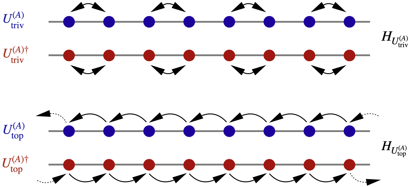
Figure 1: Illustration of the actions of the two example class A unitaries (66a)-(66b) and of the class AIII Hamiltonians (74e)-(74h) that they map to under (27).

VI.1.2 Unitaries with chiral symmetry

The only remaining nontrivial case in 1D is class DIII, which maps to class D for Hamiltonians [c.f. (64)]. Topological Hamiltonians in class D are exemplified by the well-known $p$-wave superconducting chain Kitaev (2001). We take this as our starting point and use our one-to-one mapping to obtain a nontrivial unitary in class DIII.

The Hamiltonian for the $p$-wave superconductor may be written as Kitaev (2001)

$$\hat{H}_{\rm K} = -\mu\sum_{j}\left[c^{\dagger}_{j}c^{\phantom{\dagger}}_{j}-\frac{1}{2}\right]$$ (75)

$$-\frac{1}{2}\sum_{j}\left[tc^{\dagger}_{j}c^{\phantom{\dagger}}_{j+1}+\Delta e^{i\phi}c^{\phantom{\dagger}}_{j}c^{\phantom{\dagger}}_{j+1}+\mathrm{H.c.}\right],$$

where $\mu$ is the chemical potential, $t$ is the hopping parameter, and $\Delta e^{i\phi}$ is the superconducting pairing strength. We consider the two easily solvable (and flattened) points of this model as examples of trivial and topological flattened Hamiltonians from class D. In BdG form and in momentum space, these fixed points have the Hamiltonians

$$H^{\rm(D)}_{\rm triv}(k) =\left(\begin{array}[]{cc}1&0\\ 0&-1\end{array}\right),$$ (76c)

$$H^{\rm(D)}_{\rm top}(k) =\left(\begin{array}[]{cc}-\cos(k)&i\sin(k)\\ -i\sin(k)&\cos(k)\end{array}\right),$$ (76f)

which each (it may be verified) square to the identity matrix and satisfy PHS with $\mathcal{C}=\mathcal{K}\sigma_{x}$ [c.f. Eq. (9b)]. (These fixed point Hamiltonians also have additional symmetries, but they do not affect the arguments below.) It may also be verified (e.g., by transforming to the Majorana fermion basis and calculating the Pfaffian Kitaev (2001)) that these Hamiltonians have invariants $0$ and $1$, respectively.

We now map these Hamiltonians to unitaries using Eq. (56). Following the approach described there [c.f. also Eq. (58)], we define the CS operator as $S=\sigma_{z}$. Then these two Hamiltonians map to:

$$U_{\text{triv}}^{(\rm DIII)}(k) =\left(\begin{array}[]{cccc}1&0\\ 0&1\end{array}\right),$$ (77c)

$$U_{\text{top}}^{(\rm DIII)}(k) =\left(\begin{array}[]{cccc}-\cos(k)&i\sin(k)\\ i\sin(k)&-\cos(k)\end{array}\right).$$ (77f)

As a check, we note that $U_{\text{triv}}^{(\rm DIII)}(k)$ is indeed trivial because it is an identity matrix, while the nontriviality of $U_{\text{top}}^{(\rm DIII)}$ is consistent with its gapless quasienergy spectrum (which is readily calculated).

VI.2 Two examples in two dimensions

We now present two examples of topologically nontrivial unitaries in two-dimensional class AIII. We start from nontrivial Hamiltonians $H^{(\rm{A})}({\mathbf{k}})$ from class A and use the inverse mapping from Hamiltonians to unitaries to obtain topologically nontrivial $U^{(\rm AIII)}({\mathbf{k}})$. For $H^{(\rm{A})}({\mathbf{k}})$, we consider two different models of two-band Chern insulators (from Refs. Bernevig (2013); Roy ), specializing the values of the parameters such that the Hamiltonian is topologically nontrivial. In both cases, $H^{(\rm{A})}({\mathbf{k}})=\bm{\sigma}\cdot\mathbf{n}({\mathbf{k}})$ for some 3-vector $\mathbf{n}({\mathbf{k}})$.

Following the approach of Sec. V.2, we define a CS operator by $\mathcal{S}=\sigma_{z}$ (acting on the two bands). Then, applying the mapping (56) to $H^{(\rm A)}(k)$, we obtain the following unitary:

$$U^{(\rm AIII)}({\mathbf{k}})=\frac{1}{|\mathbf{n}({\mathbf{k}})|}\left(n_{z}\mathbb{I}-in_{y}\sigma_{x}+in_{x}\sigma_{y}\right),$$ (78)

where $|\mathbf{n}({\mathbf{k}})|$ appears due to the flattening of $H^{(\rm{A})}({\mathbf{k}})$.

For our first example, we let $H^{(\rm{A})}({\mathbf{k}})$ be the Hamiltonian given by Eq. (8.17) in Ref. Bernevig (2013). Setting the parameters there to $M=-3$ and $B=-1$ yields $\mathbf{n}({\mathbf{k}})=(\sin k_{x},\sin k_{y},1+\cos k_{x}+\cos k_{y})$. Then, the Chern number of $H^{(\rm{A})}({\mathbf{k}})$ is $1$ Bernevig (2013). The numerical computation of the quasienergy spectrum of the unitary given by Eq. (78) reveals a Dirac cone (Fig. 2).

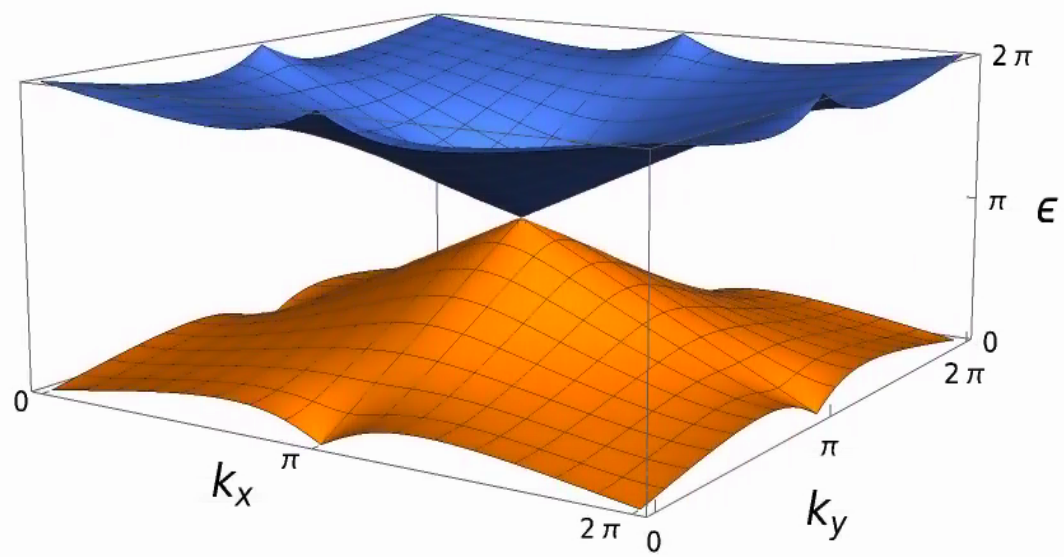
Figure 2: Three-dimensional view of the quasienergy spectrum of the unitary $U^{(\rm{AIII})}(k)$ obtained from the Chern insulator Hamiltonian in Ref. Bernevig (2013).

For our second example, we let $H^{(\rm{A})}({\mathbf{k}})$ be the Hamiltonian given by Eq. (1) of Ref. Roy . Setting the parameters there to $a=t=1,\Phi=\pi/2,\gamma_{1}=0$, and $\gamma_{2}=\pi$, we obtain $\mathbf{n}({\mathbf{k}})=(2(\sqrt{2}\cos k_{x}+\cos k_{y}),-\sqrt{2}\cos k_{x},M+2t_{2}\sin k_{x}\sin k_{y})$, where $t_{2}$ and $M$ are real parameters . The Chern number of $H^{(\rm{A})}({\mathbf{k}})$ is then equal to $1$ if $|M|<t_{2}$ and zero otherwise Roy . Thus, Eq. (78) with $|M|<t_{2}$ provides another example of a nontrivial unitary in two-dimensional class AIII.

VII Conclusion

In this work, we presented a topological classification of non-interacting, local unitaries in all dimensions and symmetry classes based on equivalence up to local generatability. To achieve this, we defined the notion of equivalence up to local generatability in the presence of symmetry, and we showed that it is equivalent to homotopy equivalence. We then used a one-to-one, homotopy-preserving mapping between unitaries and Hamiltonians to read off, from the existing classification of Hamiltonians, the classification of unitaries up to HE, and thus also up to LGE. (More precisely we used a more general notion of stable HE based on K-theoretic stable homotopy from the translation invariant case.)

Our work opens several natural directions for future study. The one-to-one correspondence between unitaries and static Hamiltonians can be used both to generate more examples of topologically nontrivial unitaries and to find explicit formulas for topological invariants (by transforming a known invariant from the static case). We presented some examples of this approach in Sec. VI, but there are many more AZ symmetry classes to explore in this way. Another follow-up to our work would be to determine a precise bulk-boundary correspondence between $(d+1)$-dimensional Floquet operators restricted to the edge and $d$-dimensional local unitaries.

While we have focused throughout on the non-interacting case, we note that progress has been made recently in related problems in the interacting case, including the construction of nontrivial quantum cellular automata in dimensions higher than one Haah et al. (2023) and the classification of translation-invariant Clifford quantum cellular automata Haah . It would be interesting to see if the ideas developed in this paper have any extension to the interacting case.

Appendix A Composition preserves symmetry

We verify that the composition operation defined in Eq. (35) preserves any symmetries present.

First, consider PHS. From Eq. (6b) and the antiunitarity of $\mathcal{C}$, we read off (for any times $t_{1},t_{2}$)

$$\mathcal{C}\hat{\mathcal{T}}\exp\left(-i\int_{t_{1}}^{t_{2}}dt\ H(t)\right)\mathcal{C}^{-1}=\hat{\mathcal{T}}\exp\left(-i\int_{t_{1}}^{t_{2}}dt\ H(t)\right).$$ (79)

Thus,

$$\mathcal{C}(U\star U_{\text{LG}})\mathcal{C}^{-1}=\left[\hat{\mathcal{T}}\exp\left(-i\int_{1/2}^{1}dt\ H(t)\right)\right]\mathcal{C}U\mathcal{C}^{-1}\hat{\mathcal{T}}\left(-i\int_{0}^{1/2}dt\ H(t)\right)=U\star U_{\text{LG}},$$ (80)

by Eq. (18b). Thus, $U\star U_{\text{LG}}$ has PHS.

For the cases of CS and TRS, and also for later calculations, it is useful to show the following two identities. Consider a symmetry class $\mathbb{S}$ with CS, TRS, or both, and define the symmetry class $X$ by Eq. (36). If $\mathbb{S}$ has CS, then the composition of any $U$ in $\mathbb{S}$ with any $U_{\text{LG}}$ that is locally generated in $\mathbb{S}$ [by some $H(t)$] may be written as

$$U\star U_{\text{LG}}=\mathcal{S}U_{\text{LG}}^{(X)\dagger}\mathcal{S}^{-1}UU_{\text{LG}}^{(X)},$$ (81)

where $U_{\text{LG}}^{(X)}$ is locally generated in $X$ by $H^{(X)}(t)=\frac{1}{2}H(\frac{1}{2}t)$. Similarly, if $\mathbb{S}$ has TRS, then the composition of any $U$ in $\mathbb{S}$ with any $U_{\text{LG}}$ that is locally generated in $\mathbb{S}$ [by some $H(t)$] may be written as

$$U\star U_{\text{LG}}=\mathcal{T}U_{\text{LG}}^{(X)\dagger}\mathcal{T}^{-1}UU_{\text{LG}}^{(X)},$$ (82)

where $U_{\text{LG}}^{(X)}$ is locally generated in $X$ by $H^{(X)}(t)=\frac{1}{2}H(\frac{1}{2}t)$.

To show these two identities, we start by showing

$$\hat{\mathcal{T}}\exp\left(-i\int_{1/2}^{1}dt\ H(t)\right) =\mathcal{S}\left[\hat{\mathcal{T}}\exp\left(-i\int_{0}^{1/2}dt\ H(t)\right)\right]^{\dagger}\mathcal{S}^{-1},$$ (83a)

$$\hat{\mathcal{T}}\exp\left(-i\int_{1/2}^{1}dt\ H(t)\right) =\mathcal{T}\left[\hat{\mathcal{T}}\exp\left(-i\int_{0}^{1/2}dt\ H(t)\right)\right]^{\dagger}\mathcal{T}^{-1},$$ (83b)

which are obtained as follows. We relabel $t\to 1-t$ and use Eq. (16c) to write the left-hand side of (83a) as $\widetilde{\mathcal{T}}\exp\left[-i\int_{0}^{1/2}dt\ H(1-t)\right]=\widetilde{\mathcal{T}}\exp\left[i\int_{0}^{1/2}dt\ \mathcal{S}H(t)\mathcal{S}^{-1}\right]$ (where $\widetilde{\mathcal{T}}$ is the anti-time ordering symbol), then bring the CS operators outside the anti-time ordered exponential. Eq. (83b) is obtained similarly using Eq. (16a) and the antiunitarity of $\mathcal{T}$. Comparing Eq. (35) with Eqs. (83a)-(83b), we then obtain the two identities (81)-(82) by noting

$$U_{\text{LG}}^{(X)}=\hat{\mathcal{T}}\exp\left(-i\int_{0}^{1}dt\ \frac{1}{2}H(t/2)\right)=\hat{\mathcal{T}}\exp\left(\int_{0}^{1/2}dt\ H(t)\right),$$ (84)

in which the first equality holds by definition.

We can now confirm that composition preserves CS and TRS (if either or both is present in $\mathbb{S}$). In the case of CS, we use Eq. (81) to obtain

$$\mathcal{S}(U\star U_{\text{LG}})\mathcal{S}^{-1}=\mathcal{S}^{2}U_{\text{LG}}^{(X)\dagger}\mathcal{S}^{-1}UU_{\text{LG}}^{(X)}\mathcal{S}^{-1}=U_{\text{LG}}^{(X)\dagger}\mathcal{S}UU_{\text{LG}}^{(X)}\mathcal{S}^{-1}=U_{\text{LG}}^{(X)\dagger}U^{\dagger}\mathcal{S}U_{\text{LG}}^{(X)}\mathcal{S}^{-1}=(U\star U_{\text{LG}})^{\dagger},$$ (85)

where we obtain the second equality from Eq. (11) and the third equality from Eq. (18c). Similarly, in the case of TRS, we use Eq. (82) to obtain

$$\mathcal{T}(U\star U_{\text{LG}})\mathcal{T}^{-1}=\mathcal{T}^{2}U_{\text{LG}}^{(X)\dagger}\mathcal{T}^{-1}UU_{\text{LG}}^{(X)}\mathcal{T}^{-1}=U_{\text{LG}}^{(X)\dagger}\mathcal{T}UU_{\text{LG}}^{(X)}\mathcal{T}^{-1}=U_{\text{LG}}^{(X)\dagger}U^{\dagger}\mathcal{T}U_{\text{LG}}^{(X)}\mathcal{T}^{-1}=(U\star U_{\text{LG}})^{\dagger},$$ (86)

where we obtain the second equality by noting that

$$\mathcal{T}^{2}=(\operatorname{sgn}\mathcal{T}^{2})\mathbb{I}\text{ [hence }\mathcal{T}^{-1}=(\operatorname{sgn}\mathcal{T}^{2})\mathcal{T}\text{]},$$ (87)

and the third equality by using Eq. (18a).

Thus, we have shown that for all symmetry classes $\mathbb{S}$, the composition $U\star U_{\text{LG}}$ is in $\mathbb{S}$.

Appendix B Further details on the equivalence of LGE to HE

B.1 Classes with CS

We show that LGE is equivalent to the condition (37) in the symmetry classes $\mathbb{S}$ with CS. Then, we make provide some further details for the proof (from Sec. IV.2) that (37) is equivalent to HE.

Consider the symmetry classes with CS. If two unitaries $U_{0}$ and $U_{1}$ are LGE, then by definition we have $U_{1}=U_{0}\star U_{\text{LG}}$ for some $U_{\text{LG}}$ that is locally generated in $\mathbb{S}$, and then Eq. (37) holds by the identity (81).

Conversely, suppose that $U_{0}$ and $U_{1}$ are related by Eq. (37) for some $U_{\text{LG}}^{(X)}$ that is locally generated in $X$. By assumption, there is some $H^{(X)}(t)$ in $X$ that generates $U_{\text{LG}}^{(X)}$. We then define

$$H(t)=\begin{cases}2H^{(X)}(2t)&0\leq t<1/2,\\ -2\mathcal{S}H^{(X)}(2-2t)\mathcal{S}^{-1}&1/2<t\leq 1.\end{cases}$$ (88)

There is no need to define $H(t)$ at the specific point $t=1/2$, since this point is a set of measure zero in the integration that appears in the time-ordered exponential.

We claim that $H(t)$ is in $\mathbb{S}$. To see this, first recall that $X$ has PHS if and only if $\mathbb{S}$ does. It is clear from Eq. (16b) that $H(t)$ inherits PHS from $H^{(X)}(t)$ if present. It is also straightforward to verify, using Eq. (11), that $H(t)$ has CS [Eq. (16c)]. TRS, if present, follows immediately because it is a combination of CS and PHS.

We then define $U_{\text{LG}}$ to be generated by $H(t)$. By construction, we have $H^{(X)}(t)=\frac{1}{2}H(\frac{1}{2}t)$ for $0\leq t\leq 1$. Thus, by the identity (81), we have $U_{0}\star U_{\text{LG}}=\mathcal{S}U_{\text{LG}}^{(X)\dagger}\mathcal{S}^{-1}U_{0}U_{\text{LG}}^{(X)}$, which shows that $U_{0}$ and $U_{1}$ are LGE. This completes the proof that LGE is equivalent to the condition (37) in the symmetry classes with CS.

Let us make one comment on this proof. If we take (37) as given, we have some $H^{(X)}(t)$ that generates $U_{\text{LG}}^{(X)}$ (by assumption), and we construct $U_{\text{LG}}$ as being generated by $H(t)$ [defined by (88)]. If we then take this $U_{\text{LG}}$ as the input to our proof that LGE implies (37), the $H^{(X)}(t)$ that we construct will be identical to the original $H^{(X)}(t)$ if we choose to generate $U_{\text{LG}}$ with $H(t)$. However, this agreement is not essential to the proof; we could in principle generate $U_{\text{LG}}$ by some $H^{\prime}(t)$ that differs from $H(t)$, and then the quantity $H^{{}^{\prime}(X)}(t)=\frac{1}{2}H^{\prime}(\frac{1}{2}t)$ that is constructed in the proof would differ from $H^{(X)}(t)$.

Next, we provide some further comments on the proof that (37) is equivalent to HE.

We can confirm that $U_{\text{LG}}^{{}^{\prime}(X)}$ is generated by $-\mathcal{S}h^{(X)}(1-t)\mathcal{S}^{-1}$ as follows:

$$U_{\text{LG}}^{{}^{\prime}(X)} =\mathcal{S}\left\{\hat{\mathcal{T}}\exp[-i\int_{0}^{1}dt\ h^{(X)}(t)]\right\}^{\dagger}\mathcal{S}^{-1}$$ (89a)

$$=\mathcal{S}\hat{\mathcal{T}}\exp[i\int_{0}^{1}dt\ h^{(X)}(1-t)]\mathcal{S}^{-1},$$ (89b)

where the first equality holds by definition and the second by relabelling $t\to 1-t$. Then, we only need to bring the CS operators inside the time-ordered exponential.

In the proof that (37) is equivalent to HE, it is important to note that the $U_{\text{LG}}^{(X)}$ in (37) need not be unique. To make this point more explicit, consider taking (37) as given; then, we have some $H^{(X)}(t)$ that (by assumption) generates $U_{\text{LG}}^{(X)}$, and we use this $H^{(X)}(t)$ to construct the homotopy (39). If we take this homotopy as the input to our proof that HE implies (37), we obtain $U_{\text{LG}}^{{}^{\prime}(X)}$ generated by $H^{{}^{\prime}(X)}(t)=-\mathcal{S}h^{(X)}(1-t)\mathcal{S}^{-1}=-\frac{1}{2}i(\partial_{t}U^{\dagger})(1-t)U(1-t)$, which seem to differ from $U_{\text{LG}}^{(X)}$ and $H^{(X)}(t)$. However, for our purpose of showing that LGE and HE are equivalent, the $U_{\text{LG}}^{(X)}$ that appears in (37) need not be unique, and even if it is unique, the Hamiltonian that generates it need not be unique.

B.2 Classes with TRS

We start by showing that LGE is equivalent to the condition (44) in the symmetry classes $\mathbb{S}$ with TRS. LGE (of two unitaries $U_{0}$ and $U_{1}$) immediately implies Eq. (44) due to the identity (82). Conversely, if we instead assume Eq. (44), then we define

$$H(t)=\begin{cases}2H^{(X)}(2t)&0\leq t<1/2,\\ -2\mathcal{T}H^{(X)}(2-2t)\mathcal{T}^{-1}&1/2<t\leq 1.\end{cases}$$ (90)

As in the CS case [Appendix B.1], it is straightforward to verify that $H(t)$ is in $\mathbb{S}$ [now using Eq. (87)]. Then we again define $U_{\text{LG}}$ to be generated by $H(t)$, and we obtain $U_{0}\star U_{\text{LG}}=\mathcal{T}U_{\text{LG}}^{(X)\dagger}\mathcal{T}^{-1}U_{0}U_{\text{LG}}^{(X)}$ using the identity (82).

We proceed to show that HE (in a class $\mathbb{S}$ with TRS) is equivalent to the condition (44), following the same approach as in Sec. IV.2. One direction is trivial: given (44), we follow exactly the same steps as in the paragraph above Eq. (39), now using the $U_{\text{LG}}^{(X)}$ that appears in (44); then (39) (with $\mathcal{S}$ replaced by $\mathcal{T}$) is the required homotopy. We may readily verify that $U(s)$ has PHS (if present). Also, $U(s)$ has TRS, as we can see from a calculation very similar to (86). Thus, $U(s)$ is in the given symmetry class $\mathbb{S}$.

It remains to show the other direction: that HE implies (44). Given a homotopy $U(s)$ that connects $U_{0}$ to $U_{1}$, we define $h^{(X)}(s)$ by Eq. (40), where the class $X$ is given by Eq. (36). The same argument as given below Eq. (40) shows that $h^{(X)}(s)$ ($0\leq s\leq 1$) is a local Hamiltonian in class $X$.

By construction, we have $i\partial_{s}U(s)=2ih^{(X)}(s)U(s)$. We also have $i\partial_{s}U(s)=2U(s)\mathcal{T}h^{(X)}(s)\mathcal{T}^{-1}$; to see this, we note that $\mathcal{T}h^{(X)}(s)\mathcal{T}^{-1}=-2i[\partial_{s}U^{\dagger}(s)]U(s)=2iU^{\dagger}(s)\partial_{s}U(s)$, where the first equality holds by the TRS of $U(s)$ (and the homotopy being “sufficiently nice” to allow commuting $S$ with the derivative) and the second equality holds because $U^{\dagger}(s)U(s)=\mathbb{I}$. Adding these equations yields

$$i\frac{\partial U(s)}{\partial s}=h^{(X)}(s)U(s)+U(s)\mathcal{T}h^{(X)}(s)\mathcal{T}^{-1}.$$ (91)

The key point is that Eq. (91), being a first-order differential equation, has a unique solution given the initial condition $U(0)=U_{0}$. We can therefore obtain a convenient formal solution by making an ansatz and checking that it works.

Our ansatz is

$$U(s)=u_{\text{LG}}^{(X)}(s)U_{0}\mathcal{T}u_{\text{LG}}^{(X)\dagger}(s)\mathcal{T}^{-1},$$ (92)

where $u_{\text{LG}}^{(X)}(s)$ is generated by $h^{(X)}(t)$ from $t=0$ to $s$. Then $u_{\text{LG}}^{(X)}(0)=\mathbb{I}$, so $U(0)=U_{0}$, as required. The differential equation (91) holds due to $i\partial_{s}u_{\text{LG}}^{(X)}=h^{(X)}(s)u_{\text{LG}}^{(X)}(s)$ (and the adjoint of this equation); c.f. the antiunitarity of $\mathcal{T}$. Thus, Eq. (92) is a valid expression for the given homotopy $U(s)$.

We have therefore shown

$$U_{1}=u_{\text{LG}}^{(X)}U_{0}\mathcal{T}u_{\text{LG}}^{(X)\dagger}\mathcal{T}^{-1},$$ (93)

where $u_{\text{LG}}^{(X)}\equiv u_{\text{LG}}^{(X)}(1)$ is locally generated in class $X$. As we now show, this form for $U_{1}$ is the same as (44) up to trivial transformations. We define $U_{\text{LG}}^{{}^{\prime}(X)}=\mathcal{T}u_{\text{LG}}^{(X)\dagger}\mathcal{T}^{-1}$; then $U_{1}=\mathcal{T}^{-1}U_{\text{LG}}^{{}^{\prime}(X)\dagger}\mathcal{T}U_{0}U_{\text{LG}}^{(X)}$, which establishes Eq. (44) [c.f. Eq. (87)]. Note that $U_{\text{LG}}^{{}^{\prime}(X)}$ is generated by $H^{{}^{\prime}(X)}(t)\equiv\frac{1}{2}\mathcal{T}h^{(X)}(1-t)\mathcal{T}^{-1}$ and is thus locally generated in class $X$. We can see this from Eqs. (89a)-(89b) with $\mathcal{T}$ replacing $\mathcal{S}$ (note that the sign inside the exponent will flip sign in this case once we bring the TRS operators past the $i$). This completes the proof of the equivalence of HE to (44), and thus also of HE to LGE in the classes with TRS.

Appendix C Classification with restricted number of orbitals

In this section, we show that restricting the number of generalized orbitals to be even or to be a multiple of four [according to (55)] has no effect on the classification of Hamiltonians. Although we only need to consider the symmetry classes A, AI, and AII, the argument is more clearly presented considering a general symmetry class.

Write $\mathcal{H}^{\mathbb{S}}$ for the set of gapped, local Hamiltonians in symmetry class $\mathbb{S}^{\prime}$, and write $\mathcal{H}_{r}^{\mathbb{S}^{\prime}}$ for the subset for which the number of generalized orbitals is restricted to be a multiple of four (later we also treat the case of restriction to an even number). We have already discussed the notions of homotopy equivalence ($\approx)$ and stable homotopy equivalence ($\sim$) on $\mathcal{H}^{\mathbb{S}^{\prime}}$ in Sec. II.3. We define homotopy equivalence ($\overset{r}{\approx}$) and stable homotopy equivalence ($\overset{r}{\sim}$) on $\mathcal{H}_{r}^{\mathbb{S}^{\prime}}$ in the same way with the additional requirements that the homotopy $H(s)$ and the trivial Hamiltonians $H_{0}^{(0)}$ and $H_{1}^{(0)}$ [in Eq. (14)] must be in $\mathcal{H}_{r}^{\mathbb{S}^{\prime}}$.

Our task is to show that two Hamiltonians in the restricted space $\mathcal{H}_{r}^{\mathbb{S}^{\prime}}$ are equivalent up to stable homotopy within $\mathcal{H}_{r}^{\mathbb{S}^{\prime}}$ if and only if they are equivalent up to stable homotopy within the larger set $\mathcal{H}^{\mathbb{S}^{\prime}}$. That is, we must show

$$H_{0}\overset{r}{\sim}H_{1}\text{ if and only if }H_{0}\sim H_{1}.$$ (94)

This equivalence implies that the Hamiltonians in $\mathcal{H}_{r}^{\mathbb{S}^{\prime}}$ have the same classification as the Hamiltonians in $\mathcal{H}^{\mathbb{S}^{\prime}}$.

One direction of the equivalence is immediate: if $H_{0}\overset{r}{\sim}H_{1}$, then $H_{0}\sim H_{1}$, because the homotopy that connects $H_{0}\oplus H_{0}^{(0)}$ and $H_{1}\oplus H_{1}^{(0)}$ within $\mathcal{H}_{r}^{\mathbb{S}^{\prime}}$ is also a homotopy within $\mathcal{H}^{\mathbb{S}^{\prime}}$ (since $\mathcal{H}_{r}^{\mathbb{S}^{\prime}}$ is a subset of $\mathcal{H}^{\mathbb{S}^{\prime}}$).

To show the other direction, consider $H_{0}$ and $H_{1}$ in $\mathcal{H}_{r}^{\mathbb{S}^{\prime}}$ with $H_{0}\overset{r}{\sim}H_{1}$. The number of generalized orbitals for $H_{0}$ and $H_{1}$ is $4n_{0}$ and $4n_{1}$, respectively (for some integers $n_{0},n_{1}$). By assumption, there are trivial Hamiltonians $H_{0}^{(0)}$ and $H_{1}^{(0)}$ (with $\alpha_{0}$ and $\alpha_{1}$ generalized orbitals, respectively) for which $H_{0}\oplus H_{0}^{(0)}\approx H_{1}\oplus H_{1}^{(0)}$. Then there is a homotopy $H(s)$, with $4n_{0}+\alpha_{0}=4n_{1}+\alpha_{1}$ generalized orbitals, from $H_{0}\oplus H_{0}^{(0)}$ to $H_{1}\oplus H_{1}^{(0)}$.

If $\alpha_{0}$ is a multiple of four, then so is $\alpha_{1}$, and $H(s)$ is then the required homotopy within $\mathcal{H}_{r}^{\mathbb{S}^{\prime}}$. Otherwise, let $\alpha^{\prime}\geq 1$ be any integer for which $\alpha_{0}+\alpha^{\prime}$ is a multiple of four, and let $H^{\prime}$ be a trivial Hamiltonian in $\mathbb{S}^{\prime}$ with $\alpha^{\prime}$ generalized orbitals. (For $\mathbb{S}^{\prime}=$AII, the number of generalized orbitals is always even, so $\alpha^{\prime}=2$ suffices.) Then $H_{0}^{(0)}\oplus H^{\prime}$ and $H_{1}^{(0)}\oplus H^{\prime}$ are trivial Hamiltonians in $\mathcal{H}_{r}^{\mathbb{S}}$, and we can define the following homotopy from $H_{0}\oplus H_{0}^{(0)}\oplus H^{\prime}$ to $H_{1}\oplus H_{1}^{(0)}\oplus H^{\prime}$:

$$H_{r}(s)=H(s)\oplus H^{\prime},$$ (95)

which has $4n_{0}+\alpha_{0}+\alpha^{\prime}$ generalized orbitals and thus is in $\mathcal{H}_{r}^{\mathbb{S}^{\prime}}$. This homotopy implies $H_{0}\overset{r}{\sim}H_{1}$, which completes the proof of (94).

We can also define $\mathcal{H}_{r}^{\mathbb{S}^{\prime}}$ to be the subset of $\mathcal{H}_{r}^{\mathbb{S}^{\prime}}$ with the number of generalized orbitals defined to be even. Then, repeating the same argument with $\alpha_{0}+\alpha^{\prime}$ only required to be even, we may show the same equivalence (94) for the case in which the Hamiltonians are restricted to have an even number of orbitals rather than a multiple of four. Thus, we conclude that the restrictions (55) that we made in order to define an inverse to $H_{U}$ do not affect the topological classification.

Finally, we note that, just as in the case of $\mathcal{H}^{\mathbb{S}^{\prime}}$, there is no effect on the classification if we restrict our attention to the subset of flattened Hamiltonians within $\mathcal{H}_{r}^{\mathbb{S}^{\prime}}$. It is on this subset that the inverse to $H_{U}$ is defined.

Appendix D Mapping between unitaries and Hamiltonians preserves stable homotopy

In this section, we verify that, in each symmetry class, the one-to-one mapping $U\mapsto H_{U}$ preserves equivalence up to stable homotopy [that is, we verify (34)]. In particular, we are considering here two unitaries that are in the same symmetry class $\mathbb{S}$, but that may have different numbers of generalized orbitals. Equivalently, since the mapping is one-to-one, we can consider two Hamiltonians in the same symmetry class $\mathbb{S}^{\prime}$ (which is related to $\mathbb{S}$ according to Table 2), possibly with different numbers of generalized orbitals. In the cases $\mathbb{S}^{\prime}=$A, AI, or AII, we understand each instance of $\sim$ and $\approx$ below to in fact refer to the corresponding equivalences $\overset{r}{\sim}$ and $\overset{r}{\approx}$ within the restricted space $\mathcal{H}_{r}^{\mathcal{S}^{\prime}}$ that has the condition (55) imposed on the number of generalized orbitals [see Appendix C].

There are two cases to consider: the five symmetry classes $\mathbb{S}$ that do not have CS (equivalently, the five $\mathbb{S}^{\prime}$ that do), and the five symmetry classes $\mathbb{S}$ that have CS (equivalently, the five $\mathbb{S}^{\prime}$ that do not). In each case, we first verify that the mapping preserves HE, that is,

$$U_{0}\approx U_{1}\iff H_{U_{0}}\approx H_{U_{1}},$$ (96)

in which $U_{0}$ and $U_{1}$ have the same number of generalized orbitals (or equivalently, $H_{U_{0}}$ and $H_{U_{1}}$ have the same number, which is greater by a factor of two in the case that the unitaries do not have CS). We then use (96) to obtain the desired result (34).

If $\mathbb{S}$ is one of the five classes without CS, then the mapping is given by Eq. (27). Suppose $U_{0}\approx U_{1}$. Then we may use the homotopy $U(s)$ between $U_{0}$ and $U_{1}$ to define a family of local Hamiltonians using the mapping (27):

$$H(s)=\begin{pmatrix}0&U(s)\\ U^{\dagger}(s)&0\end{pmatrix},$$ (97)

which, by construction, is a homotopy between $U_{H_{0}}$ and $U_{H_{1}}$. From Sec. V.1 we know that $H(s)$ has the appropriate symmetries [note that $U(s)$ by assumption has the same symmetries as $U_{0}$ and $U_{1}$]. Thus, $H_{U_{0}}\approx H_{U_{1}}$. Conversely, given two flattened, local, HE Hamiltonians in a symmetry class $\mathcal{S}^{\prime}$ with CS, we have unique $U_{0}$, $U_{1}$ for which the two Hamiltonians are equal to $H_{U_{0}}$ and $H_{U_{1}}$. The given homotopy $H(s)$ between $H_{U_{0}}$ and $H_{U_{1}}$ then maps (under the inverse mapping $H\mapsto H_{U}$) to a homotopy $U(s)$ given by (97), and, as shown in Sec. V.1, $U(s)$ is local and has the appropriate symmetries. Thus, $U_{0}\approx U_{1}$, and so (96) is obtained for all $\mathbb{S}$ without CS.

If $\mathbb{S}$ is one of the five classes with CS, then the mapping is given by Eq. (53). Similar to the argument in the previous paragraph, we define

$$H(s)=SU(s),$$ (98)

where we either take (a) $U(s)$ to be a homotopy between $U_{0}$ and $U_{1}$ (supposing we are given $U_{0}\approx U_{1}$), or (b) $H(s)$ to be a given homotopy between $H_{U_{0}}$ and $H_{U_{1}}$ (supposing we are given $H_{U_{0}}\approx H_{U_{1}}$). In case (b), the homotopy $U(s)$ is defined by the inverse mapping, i.e., $U(s)=SH(s)$. We thus obtain (96) in the remaining five symmetry classes.

One immediate consequence of (96) is that a unitary is trivial (i.e., HE to the identity) if and only if the corresponding Hamiltonian is trivial. To obtain the desired result (34), it then suffices to show:

$$H_{U_{0}\oplus U_{1}}=H_{U_{0}}\oplus H_{U_{1}},$$ (99)

in which $U_{0}$ and $U_{1}$ are arbitrary local unitaries in the same symmetry class. (We only need the special case in which one of these unitaries is trivial, but the general case is no more difficult.) Eq. (99) follows immediately from the definitions (27) and (53), because we indeed have

$$\begin{pmatrix}0&U_{0}\oplus U_{1}\\ (U_{0}\oplus U_{1})^{\dagger}&0\end{pmatrix} =\begin{pmatrix}0&U_{0}\\ U_{0}^{\dagger}&0\end{pmatrix}\oplus\begin{pmatrix}0&U_{1}\\ U_{1}^{\dagger}&0\end{pmatrix},$$ (100a)

$$S(U_{0}\oplus U_{0}) =(SU_{1})\oplus(SU_{1}).$$ (100b)

From (96) and (99), which we have shown in all symmetry classes, we immediately obtain

$$U_{0}\oplus U_{0}^{(0)}\approx U_{1}\oplus U_{1}^{(0)}\iff H_{U_{0}\oplus U_{0}^{(0)}}\approx H_{U_{1}\oplus U_{1}^{(0)}}\iff H_{U_{0}}\oplus H_{U_{0}^{(0)}}\approx H_{U_{1}}\oplus H_{U_{1}^{(0)}},$$ (101)

which demonstrates (34) in all symmetry classes.

Appendix E Canonical forms for symmetry operators

In this section, we present the basis transformations that bring the symmetry operators (in the four symmetry classes with both TRS and PHS) from their standard forms to the forms that we used in the main text.

TRS and PHS can be written as

$$\mathcal{T}=\mathcal{K}U_{\mathcal{T}},\ \mathcal{C}=\mathcal{K}U_{\mathcal{C}},$$ (102)

where $\mathcal{K}$ is complex conjugation and $U_{\mathcal{T}}$ and $U_{\mathcal{C}}$ are unitary. From Eq. (7), the CS operator is then given by

$$\mathcal{S}=e^{i\delta}U_{\mathcal{C}}^{*}U_{\mathcal{T}}.$$ (103)

Complex conjugation is defined relative to a certain basis. Under a change of basis by a unitary matrix $V$, the unitary matrices $U_{\mathcal{T}}$ and $U_{\mathcal{C}}$ transform as

$$U_{\mathcal{T}}\to V^{*}U_{\mathcal{T}}V^{\dagger},\ U_{\mathcal{C}}\to V^{*}U_{\mathcal{C}}V^{\dagger},$$ (104)

where the star appears due to $\mathcal{K}$.

In Table 4, we present the changes of basis needed to obtain the canonical forms used in the main text. The “starting forms” are taken from Table I of Ref. Roy and Harper (2017). In three of the symmetry classes, two different basis transformations are presented because different forms are needed for Hamiltonians and for unitaries. From Eq. (103), it may be verified that the CS operator in the new basis is $\mathcal{S}=\sigma_{z}\otimes\mathbb{I}$ (up to a phase) in each case.

Table 4: Basis transformations for TRS and PHS in the four symmetry classes where both are present.

	Starting forms		Change of basis	New forms
AZ class	$U_{\mathcal{T}}$	$U_{\mathcal{C}}$	$V$	$V^{*}U_{\mathcal{T}}V^{\dagger}$	$V^{*}U_{\mathcal{C}}V^{\dagger}$
BDI	$\mathbb{I}$	$\sigma_{x}\otimes\mathbb{I}$	$\frac{1}{\sqrt{2}}\begin{pmatrix}1&0&1&0\\ 0&1&0&1\\ -1&0&1&0\\ 0&-1&0&1\end{pmatrix}$	$\mathbb{I}$	$\sigma_{z}\otimes\mathbb{I}$
			$\frac{1}{\sqrt{2}}\begin{pmatrix}0&1&0&1\\ 1&0&1&0\\ -i&0&i&0\\ 0&-i&0&i\end{pmatrix}$	$\sigma_{z}\otimes\mathbb{I}$	$\mathbb{I}$
DIII	$\mathbb{I}\otimes i\sigma_{y}$	$\sigma_{x}\otimes\mathbb{I}$	$\frac{1}{\sqrt{2}}\begin{pmatrix}i&0&0&1\\ 0&-i&1&0\\ -i&0&0&1\\ 0&i&1&0\end{pmatrix}$	$-\sigma_{x}\otimes i\sigma_{y}$	$\sigma_{y}\otimes i\sigma_{y}$
			$\frac{1}{\sqrt{2}}\begin{pmatrix}0&1&i&0\\ 1&0&0&-i\\ -i&0&0&1\\ 0&i&1&0\end{pmatrix}$	$\sigma_{y}\otimes\mathbb{I}$	$\sigma_{x}\otimes\mathbb{I}$
CII	$\mathbb{I}\otimes i\sigma_{y}$	$i\sigma_{y}\otimes\mathbb{I}$	$\frac{1}{\sqrt{2}}\begin{pmatrix}1&0&0&1\\ 0&-1&1&0\\ -1&0&0&1\\ 0&1&1&0\end{pmatrix}$	$-\mathbb{I}\otimes i\sigma_{y}$	$\sigma_{z}\otimes i\sigma_{y}$
			$\frac{1}{\sqrt{2}}\begin{pmatrix}0&-i&i&0\\ i&0&0&i\\ -i&0&0&i\\ 0&i&i&0\end{pmatrix}$	$-\sigma_{z}\otimes i\sigma_{y}$	$\mathbb{I}\otimes i\sigma_{y}$
CI	$\mathbb{I}$	$i\sigma_{y}\otimes\mathbb{I}$	$\frac{1}{\sqrt{2}}\begin{pmatrix}0&i&0&1\\ i&0&1&0\\ 0&-i&0&1\\ -i&0&1&0\end{pmatrix}$	$\sigma_{x}\otimes\mathbb{I}$	$i\sigma_{y}\otimes\mathbb{I}\par$

The “new forms” of Table 4, together with Eq. (102) and some trivial phase re-definitions, yield the canonical forms listed in Table 5, which are used in the main text.

Table 5: Canonical forms for TRS and PHS in the four symmetry classes where both are present.

	Unitaries		Hamiltonians
AZ class	$\mathcal{T}$	$\mathcal{C}$	$\mathcal{T}$	$\mathcal{C}$
BDI	$\mathcal{K}\sigma_{z}\otimes\mathbb{I}$	$\mathcal{K}$	$\mathcal{K}$	$\mathcal{K}\sigma_{z}\otimes\mathbb{I}$
DIII	$\mathcal{K}\sigma_{y}\otimes\mathbb{I}$	$\mathcal{K}\sigma_{x}\otimes\mathbb{I}$	$\mathcal{K}\sigma_{x}\otimes\sigma_{y}$	$\mathcal{K}\sigma_{y}\otimes\sigma_{y}$
CII	$\mathcal{K}\sigma_{z}\otimes\sigma_{y}$	$\mathcal{K}\mathbb{I}\otimes\sigma_{y}$	$\mathcal{K}\mathbb{I}\otimes\sigma_{y}$	$\mathcal{K}\sigma_{z}\otimes\sigma_{y}$
CI	$\mathcal{K}\sigma_{x}$	$\mathcal{K}\sigma_{y}$	$\mathcal{K}\sigma_{x}$	$\mathcal{K}\sigma_{y}\par$

References

- Hasan and Kane (2010) M. Z. Hasan and C. L. Kane, “Colloquium: Topological insulators,” Reviews of Modern Physics 82, 3045–3067 (2010).
- Chiu et al. (2016) Ching-Kai Chiu, Jeffrey C. Y. Teo, Andreas P. Schnyder, and Shinsei Ryu, “Classification of topological quantum matter with symmetries,” Reviews of Modern Physics 88, 035005 (2016).
- Harper et al. (2020) Fenner Harper, Rahul Roy, Mark S. Rudner, and S.L. Sondhi, “Topology and Broken Symmetry in Floquet Systems,” Annual Review of Condensed Matter Physics 11, 345–368 (2020).
- Eckardt (2017) André Eckardt, “Colloquium: Atomic quantum gases in periodically driven optical lattices,” Reviews of Modern Physics 89, 011004 (2017).
- Jotzu et al. (2014) Gregor Jotzu, Michael Messer, Rémi Desbuquois, Martin Lebrat, Thomas Uehlinger, Daniel Greif, and Tilman Esslinger, “Experimental realization of the topological Haldane model with ultracold fermions,” Nature 515, 237–240 (2014).
- Esmann et al. (2018) M. Esmann, F. R. Lamberti, A. Lemaître, and N. D. Lanzillotti-Kimura, “Topological acoustics in coupled nanocavity arrays,” Physical Review B 98, 161109 (2018).
- Yang et al. (2015) Zhaoju Yang, Fei Gao, Xihang Shi, Xiao Lin, Zhen Gao, Yidong Chong, and Baile Zhang, “Topological Acoustics,” Physical Review Letters 114, 114301 (2015).
- Ozawa et al. (2019) Tomoki Ozawa, Hannah M. Price, Alberto Amo, Nathan Goldman, Mohammad Hafezi, Ling Lu, Mikael C. Rechtsman, David Schuster, Jonathan Simon, Oded Zilberberg, and Iacopo Carusotto, “Topological photonics,” Reviews of Modern Physics 91, 015006 (2019).
- Gross et al. (2012) D. Gross, V. Nesme, H. Vogts, and R. F. Werner, “Index Theory of One Dimensional Quantum Walks and Cellular Automata,” Communications in Mathematical Physics 310, 419–454 (2012).
- Cedzich et al. (2016) C Cedzich, F A Grünbaum, C Stahl, L Velázquez, A H Werner, and R F Werner, “Bulk-edge correspondence of one-dimensional quantum walks,” Journal of Physics A: Mathematical and Theoretical 49, 21LT01 (2016).
- Cedzich et al. (2018) C. Cedzich, T. Geib, F. A. Grünbaum, C. Stahl, L. Velázquez, A. H. Werner, and R. F. Werner, “The Topological Classification of One-Dimensional Symmetric Quantum Walks,” Annales Henri Poincaré 19, 325–383 (2018).
- Cirac et al. (2017) J. Ignacio Cirac, David Perez-Garcia, Norbert Schuch, and Frank Verstraete, “Matrix product unitaries: Structure, symmetries, and topological invariants,” Journal of Statistical Mechanics: Theory and Experiment 2017, 083105 (2017).
- Higashikawa et al. (2019) Sho Higashikawa, Masaya Nakagawa, and Masahito Ueda, “Floquet chiral magnetic effect,” Physical Review Letters 123, 066403 (2019).
- Farrelly (2020) Terry Farrelly, “A review of Quantum Cellular Automata,” Quantum 4, 368 (2020).
- Cedzich et al. (2021) C. Cedzich, T. Geib, A. H. Werner, and R. F. Werner, “Chiral Floquet Systems and Quantum Walks at Half-Period,” Annales Henri Poincaré 22, 375–413 (2021).
- (16) Jeongwan Haah, arXiv:2205.09141.
- Kitaev (2006) Alexei Kitaev, “Anyons in an exactly solved model and beyond,” Annals of Physics 321, 2–111 (2006).
- Chen et al. (2010) Xie Chen, Zheng-Cheng Gu, and Xiao-Gang Wen, “Local unitary transformation, long-range quantum entanglement, wave function renormalization, and topological order,” Physical Review B 82, 155138 (2010).
- Roy and Harper (2017) Rahul Roy and Fenner Harper, “Periodic table for Floquet topological insulators,” Physical Review B 96, 155118 (2017).
- Liu (2020) Xu Liu, Classification of Static and Driven Topological Insulators, Ph.D. thesis, UCLA (2020).
- Graf and Tauber (2018) Gian Michele Graf and Clément Tauber, “Bulk–Edge Correspondence for Two-Dimensional Floquet Topological Insulators,” Annales Henri Poincaré 19, 709–741 (2018).
- Kitaev (2009) Alexei Kitaev, “Periodic table for topological insulators and superconductors,” AIP Conference Proceedings 1134, 22–30 (2009).
- Altland and Zirnbauer (1997) Alexander Altland and Martin R. Zirnbauer, “Nonstandard symmetry classes in mesoscopic normal-superconducting hybrid structures,” Physical Review B 55, 1142–1161 (1997).
- Katsura and Koma (2018) Hosho Katsura and Tohru Koma, “The noncommutative index theorem and the periodic table for disordered topological insulators and superconductors,” Journal of Mathematical Physics 59, 031903 (2018).
- (25) Jui-Hui Chung and Jacob Shapiro, arXiv.2306.00268.
- Prodan and Schulz-Baldes (2016) Emil Prodan and Hermann Schulz-Baldes, Bulk and Boundary Invariants for Complex Topological Insulators, Mathematical Physics Studies (Springer International Publishing, Cham, 2016).
- Liu et al. (2018) Xu Liu, Fenner Harper, and Rahul Roy, “Chiral flow in one-dimensional Floquet topological insulators,” Physical Review B 98, 165116 (2018).
- Mondragon-Shem et al. (2014) Ian Mondragon-Shem, Taylor L. Hughes, Juntao Song, and Emil Prodan, “Topological Criticality in the Chiral-Symmetric AIII Class at Strong Disorder,” Physical Review Letters 113, 046802 (2014).
- Teo and Kane (2010) Jeffrey C. Y. Teo and C. L. Kane, “Topological defects and gapless modes in insulators and superconductors,” Physical Review B 82 (2010), 10.1103/PhysRevB.82.115120.
- Kitaev (2001) A Yu Kitaev, “Unpaired Majorana fermions in quantum wires,” Physics-Uspekhi 44, 131–136 (2001).
- Bernevig (2013) B. Andrei Bernevig, “Topological Insulators and Topological Superconductors,” in Topological Insulators and Topological Superconductors (Princeton University Press, 2013).
- (32) Rahul Roy, arXiv:cond-mat/0603271.
- Note (1) Here we have corrected typos in Eq. (1) of Ref. Roy : the second left parentheses in the first line and the last right parentheses in the second line should be deleted.
- Haah et al. (2023) Jeongwan Haah, Lukasz Fidkowski, and Matthew B. Hastings, “Nontrivial Quantum Cellular Automata in Higher Dimensions,” Communications in Mathematical Physics 398, 469–540 (2023).