A Tracking prior to Localization workflow for Ultrasound Localization Microscopy

Abstract – Ultrasound Localization Microscopy (ULM) has proven effective in resolving microvascular structures and local mean velocities at sub-diffraction-limited scales, offering high-resolution imaging capabilities. Dynamic ULM (DULM) enables the creation of angiography or velocity movies throughout cardiac cycles. Currently, these techniques rely on a Localization-and-Tracking (LAT) workflow consisting in detecting microbubbles (MB) in the frames before pairing them to generate tracks. While conventional LAT methods perform well at low concentrations, they suffer from longer acquisition times and degraded localization and tracking accuracy at higher concentrations, leading to biased angiogram reconstruction and velocity estimation. In this study, we propose a novel approach to address these challenges by reversing the current workflow. The proposed method, Tracking-and-Localization (TAL), relies on first tracking the MB and then performing localization. Through comprehensive benchmarking using both in silico and in vivo experiments and employing various metrics to quantify ULM angiography and velocity maps, we demonstrate that the TAL method consistently outperforms the reference LAT workflow. Moreover, when applied to DULM, TAL successfully extracts velocity variations along the cardiac cycle with improved repeatability. The findings of this work highlight the effectiveness of the TAL approach in overcoming the limitations of conventional LAT methods, providing enhanced ULM angiography and velocity imaging.

Index Terms - Contrast Ultrasound, Ultrasound Localization Microscopy (ULM), super-resolution tracking.

1 INTRODUCTION

Ultrasound Localization Microscopy (ULM) enables the high-resolution imaging of blood vessels by localizing and tracking a large number of individual microbubbles (MB) injected as a contrast agent [1, 2, 3]. ULM can provide maps of the angioarchitecture along with mean flow velocities in a wide range of vessel diameters, overcoming the ultrasound diffraction limit [4, 5, 6, 7, 8, 9]. Recently, Dynamic Ultrasound Localization Microscopy (DULM) [10] has been introduced to enable the generation of super-resolved cine-loops of the vasculature. DULM can be used, e.g., to generate videos of the pulsatile blood flow in the brain [10], to map the micro angioarchitecture of the beating heart [11] and to perform functional imaging in the rodent brain [12]. Since DULM requires the localization of single MB both in space and time, it needs longer acquisitions, which could become prohibitive for clinical translation [13, 14, 15, 16]. While increasing the concentration can be used to shorten acquisition times, high concentrations of MB in ULM lead to compromised localization precision and accuracy in both angioarchitecture maps and blood flow measurements [8, 14, 15, 17].

Standard methods in ULM and DULM [2, 5, 10, 12, 14, 18, 19, 20, 21] are typically based on a localize-and-track (LAT) workflow: detect and localize MB in a frame-per-frame fashion and then use pairing algorithms to track them in the temporal dimension. While this approach works well at low concentrations, it rapidly breaks down when the number of MB per frame increases [22, 23, 24].

Moreover, ULM studies often assume that precise MB localization and high frame rate compared to the velocities of the MB enables accurate velocity estimations [2, 7, 9]. However, there is a lack of studies confirming the velocities obtained in vivo. Even in silico, the instantaneous velocities found by the tracker have not been validated. While many studies have reported issues such as the absence of a ground truth [5] or the impact of missing positions between frames, false detections and incorrect pairing can significantly bias the velocity estimation [6, 9, 13].

Kalman filtering tracking [17, 18] can also be used to inject physically consistent criteria (e.g. velocity continuity) to improve the selection and accuracy of trajectories. However, Kalman filtering is added after a standard LAT workflow.

Different approaches have been introduced either to handle the overlapping MB signals but remained limited to the imaging of the angioarchitechture [25, 23, 26, 27, 28, 29, 30, 31, 32, 24] or to separate MB into sub-populations of different velocity range [33] to reduce overlapping MB events. However, the MB separation increased the processing time and was associated with a ‘MB doubling’ effect that could bias the number of localized MB as well as the velocity [33].

Recently, a deep learning method (Deep-SMV) has been proposed for velocity recovery, with convincing results in this direction [6]. Nevertheless, the authors pointed out that the model has been trained on the velocity flows found by standard ULM approaches and that the model depends on laminar flow assumptions which might implicitly influence the model.

We propose instead to detect and segment the MB trajectories as 1-D objects in a 3D spatiotemporal volume before localizing them in a Track-and-Localize (TAL) workflow. The underlying principle is to leverage the continuity between frames, enabled by the high frame rate relative to the velocity of MB, to directly segment MB trajectories without the need for spatial and temporal separation through localization and tracking.

Herein, we demonstrate that TAL matches at low concentration and overperforms at high concentration the standard LAT approaches. Specifically, we build the theoretical framework enabling the segmentation of trajectories in three-dimensional space-time and validate its performance in silico and in vivo by benchmarking it using publicly available codes and datasets [34]. We then show that, in the context of DULM, TAL outperforms standard LAT approaches, especially at high concentration in a rat and transcranial mouse brain model. Overall, the proposed TAL method leads to systematically improved performance in terms of angioarchitecture and velocity maps and provides better and more robust cine-loops in the context of dynamic imaging.

2 METHODS

In the following we first describe our proposed TAL workflow based on a modified Hessian matrix and a thinning algorithm to segment trajectories in space-time. Then we describe the standard ULM pipeline based on the LAT workflow, which is used as a gold-standard in this study. We also describe the DULM acquisition and processing pipeline. We end this section by introducing a series of metrics to quantify the performances of the proposed methodology.

2.1 Spatiotemporal Tracking of MB Trajectories

After In-phase and Quadrature complex (IQ) image formation (i.e., beamforming) [35, 36], tissue was removed using a Singular Value Decomposition (SVD) clutter filter to recover signals from MB [37, 38]. The proposed tracking method then takes for input the envelope of the post-SVD IQ data, i.e., I(x). Inspired by [39], where the objective is to enhance tubular structures in a spatial volume, we developed a spatiotemporal filter to enhance the trajectories of the Point Spread Function (PSF) of the MB, which possess a tubular geometry in space-time. A modified Hessian matrix is calculated for each voxel of the spatiotemporal volume I(x):

$$\mathbf{H}(I)(\mathbf{x})=\lambda^{2}I(\mathbf{x})\ast\begin{pmatrix}\epsilon^{2}\frac{\partial^{2}}{\partial z^{2}}&\epsilon^{2}\frac{\partial^{2}}{\partial z\partial x}&\epsilon\frac{\partial^{2}}{\partial z\partial t}\\ \epsilon^{2}\frac{\partial^{2}}{\partial x\partial z}&\epsilon^{2}\frac{\partial^{2}}{\partial x^{2}}&\epsilon\frac{\partial^{2}}{\partial x\partial t}\\ \epsilon\frac{\partial^{2}}{\partial t\partial z}&\epsilon\frac{\partial^{2}}{\partial t\partial x}&\frac{\partial^{2}}{\partial t^{2}}\end{pmatrix}G(\mathbf{x},\lambda)$$ (1)

Where $\mathbf{x}=[z,x,t]^{T}$ are the spatiotemporal coordinates of the voxels in the volume, and $G(\mathbf{x},\lambda)=\left(\frac{1}{\sqrt{2\pi\lambda^{2}}}\right)^{3}exp\left(-\frac{\mathbf{x}^{T}\mathbf{x}}{2\lambda^{2}}\right)$ is a Gaussian kernel, where the standard deviation is defined as the width of the tubular objects, which corresponds, in our case, to the size of the PSF. While this standard deviation can be adjusted for each pixel of the image, we found that setting it to the wavelength $\lambda$ in the context of plane wave imaging yielded good results. $\epsilon>1$ is a scalar parameter that we introduced to reject potential structures that are orthogonal to the temporal dimension, which could be enhanced because of the proximity between MB in the same frame. While $\epsilon$ can, in principle, limit the measured velocities if chosen to be too large, detected tracks were not sensitive to its value. Setting $\epsilon$ to any value between 1.2 and 2 $\lambda$/frames was sufficient to regularize the tracking operation. After diagonalization of each Hessian matrix, the Jerman function [39], developed to enhance the tubular geometry structures, is applied on the three eigenvalues $(\nu_{1}\leq\nu_{2}\leq\nu_{3})$ :

$$J(\mathbf{x})=\left\{\begin{array}[]{cc}0&\nu_{2}\leq 0\text{ ou }\nu_{\rho}\leq 0\\ 1&\nu_{2}\geq\nu_{\rho}/2>0\\ \nu_{2}^{2}\left(\nu_{\rho}-\nu_{2}\right)\left(\frac{3}{\nu_{2}+\nu_{\rho}}\right)^{3}&otherwise\end{array}\right.$$ (5)

where $\nu_{\rho}$ is a regularized parametric version of $\nu_{3}$, via the $\tau\in[0,1]$ parameter, to adapt the sensitivity of the function to the non-homogeneous MB PSF trajectory’s intensity:

$$\nu_{\rho}=\left\{\begin{array}[]{cc}\nu_{3}&\nu_{3}>\tau\max_{\mathbf{x}}\nu_{3}(\mathbf{x})\\ \tau\max_{\mathbf{x}}\nu_{3}(\mathbf{x})&0<\nu_{3}\leq\tau\max_{\mathbf{x}}\nu_{3}(\mathbf{x})\\ 0&otherwise\end{array}\right.$$ (9)

After binarization, a thinning algorithm is used to segment the MB PSF trajectories centerline at a pixel resolution [40]. Thus, we obtain $N_{traj}$ tracks with a pixel precision $\{r_{1}^{i},\ldots,r_{l^{i}}^{i}\}_{i\in[|1,N_{traj}|]}$, where $r=(z,x,t)$ is the position in the space-time of a MB and $l^{i}$ is the length of the $i^{th}$ track. We kept only the $\hat{N}_{traj}$ tracks longer than $N_{f}$ frames to increase the confidence that the trajectories obtained. $\tau,\epsilon$ and $N_{f}$ are the only dataset dependent parameters. Then, from each position in each track, a localization algorithm is applied to obtain the subwavelength positions of the MB $\{\hat{r}_{1}^{i},\ldots,\hat{r}_{l^{i}}^{i}\}_{i\in[|1,\hat{N}_{traj}|]}$ (see Fig.1).

Many approaches can be used to localize the MB; here, we used the radial symmetry algorithm [34]. Finally, a function S is determined for each track by applying a cubic smoothing spline as follows:

$$\begin{array}[]{cc}S=arg\min_{S}p\sum^{l}_{j}\lVert r_{j}-S(t_{j})\rVert^{2}\\ +(1-p)\int\left\lVert\frac{d^{2}S}{dt^{2}}(t)\right\rVert^{2}dt\end{array}$$ (12)

From the Plancherel theorem, we can extract a link between the p parameter and a cut-off frequency $f_{c}:p=\frac{f_{c}^{4}}{1+f_{c}^{4}}$ as in [41] which will enforce the spatiotemporal smoothness of the trajectory. The representative function $S_{p}$ of each trajectory can be interpolated and differentiated to obtain dense trajectories and their respective velocities. The choice of the different parameters for the TAL workflow are presented in Table I.

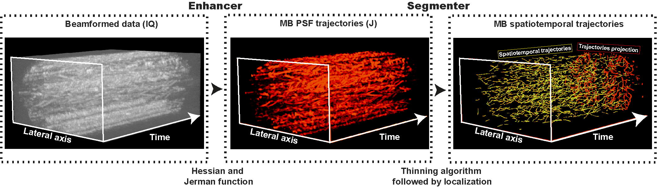
Figure 1: Localization and Tracking workflow (TAL). TAL takes a spatiotemporal (space × time) input of beamformed data, where the Jerman function is calculated (J) to extract the spatiotemporal MB PSF trajectories, before applying a thinning algorithm supported by localization algorithm to segment and super-resolve the trajectories of the moving MB

2.2 Standard LAT ULM and DULM

Standard LAT ULM was implemented using the publicly available PALA toolbox [34]. Briefly, after IQ image formation, individual MB were detected as local maxima in the B-mode images and localized using radial symmetry. The Hungarian method (Kuhn-Munkres algorithm) was used for tracking [42]. Different parameters need to be set to perform the tracking: the number of MB per frame that we consider (Nb), the Maximum Linking Distance to pair MB (MLD), the Maximum Frame Gap allowed for pairing (MFG) and the minimum length of a track $(N_{f})$ (see Table I). Then tracks were accumulated on a finer grid corresponding to approximately one tenth of the wavelength. LAT DULM was implemented following the methods of [10]. Briefly, retrospective gating on the ECG allows for the localization of MB in space and time within the cardiac cycle. LAT and TAL tracking were performed in the same manner as for static ULM, with adapted parameters as described in Table II.

2.3 In silico localization metrics

Metrics introduced in [34] and available in the PALA toolbox were used to quantify the quality of localization and detection knowing the ground truth: 1) Localization error defined as the Root Mean Square Error (RMSE) between the $i^{th}$ simulated $(z_{i}^{0},x_{i}^{0})$ and detected $(z_{i},x_{i})$ MB positions. 2) Jaccard index: $JAC=\frac{TP}{FN+TP+FP}$ , that measures the detection rate. 3) Detection precision: $Pr=\frac{TP}{FP+TP}$. 4) Detection sensitivity: $r=\frac{TP}{FN+TP}$. Where TP is the number of MB found in the $\frac{\lambda}{4}$ neighborhood of a simulated MB. FP is the number of localized MB, but where no simulated MB can be found in a $\frac{\lambda}{4}$ neighborhood. FN is the number of simulated MB where there is no localized MB to be paired within a $\frac{\lambda}{4}$-neighborhood.

2.4 In silico tracking metrics

To evaluate the performance of the tracking algorithm, we employed both local and global quality metrics. Local measurements involve assessing the accuracy of velocity estimates at specific points of interest, while global measurements involve evaluating the correlation coefficients calculated to quantify the relationship between the estimated velocities and the ground truth values.

$$\hat{C}(V_{GT},V_{map})=\frac{1}{N+1}\sum_{i=1}^{N}\left(\frac{V_{GT}^{i}-\nu_{GT}}{\sigma_{GT}}\right)\left(\frac{V_{map}^{i}-\nu_{map}}{\sigma_{map}}\right)$$ (13)

where $V_{GT}$ represents the velocity map obtained from the trajectories of the simulated positions and $V_{map}$ represents the velocity map obtained from trajectories found either by the LAT or TAL workflow. N is the number of pixels.

2.5 In vivo metrics

Resolution was evaluated using the Fourier Ring Correlation (FRC) introduced for ULM in [43]. Briefly, an estimate of the image resolution is obtained by splitting the localization dataset into two sub-images and establishing a threshold for the consistency of the frequency information. To generate the two sub-images, all the trajectories obtained with the tracker were randomly separated into two datasets. The FRC was computed by using the spatial spectra F1 and F2 of each sub-image, as follows:

$$FRC(R)=\frac{\sum_{r\in R}F_{1}(r).F_{2}(r)^{*}}{\sqrt{\sum_{r\in R}||F_{1}(r)||^{2}.\sum_{r\in R}||F_{2}(r)||^{2}}}$$ (14)

The 1/2-bit threshold was used to assert image resolution, which corresponds to the highest spatial frequency containing at least 1/2 bit of information [44].

Locally, the Full Width at Half Maximum (FWHM) was used to measure the diameter of the vessels found.

2.6 In silico validation dataset

The in silico PALA dataset is composed of 20 buffers with 1000 simulated ultrasound frames, each containing moving MB at various velocities in crossing vessels of varying sizes and shapes [34]. To achieve higher MB concentration, consecutive buffers were summed. By doing so, the number of buffers was reduced while preserving the same total number of MB simulated. The concentration (C) is presented in arbitrary units based on the number of buffers summed. C=5 a.u. means that 5 consecutives buffers have been summed to form a buffer five times more concentrated than the original ones. Note that since the total number of MB is maintained, higher concentrations are associated with shorter acquisition times.

2.7 In vivo validation dataset

The in vivo PALA dataset is composed of 240 buffers, containing 800 frames of rat brain measurements each. A craniotomy had been performed and MB were injected at $80\mu L.min^{-1}$ during 4 min [34]. As in the in silico study, the concentration was artificially increased while maintaining a constant total number of MB. Higher concentrations are thus associated with proportionally shorter acquisition times.

2.8 In vivo Dynamic ULM rat and mouse datasets

The acquisitions performed for the DULM study adhered to the guidelines outlined in the ”Guide for the Care and Use of Laboratory Animals” set forth by the Canadian Council for Animal Care. The rat study procedures were granted ethical approval by the Animal Care Ethics Committee of the Montreal Heart Institute (Permit Number: 2019-2464, 2018-32-03). Similarly, the mouse study procedures were approved by the McGill University Animal Care Committee under the regulations of Animal Use Protocol AUP-4532.

2.8.1 Rat model

The surgical procedure and ultrasound acquisitions were performed on a 500 g female adult rat under 2% isoflurane anesthesia. Throughout the procedure, the body temperature was maintained at 35 °C using a small animal monitoring platform (Labeo Technologies Inc., QC, Canada). To minimize movement, the rat’s head was secured in a stereotaxic frame, and a surgical micro drill was used to remove the skull, creating a window over the brain measuring approximately $15mm\times 10mm$.

Three datasets were obtained for the same two-dimensional plane using different concentrations. Prior to ultrasound acquisitions, an intravenous bolus injection of a MB solution ($1.2\times 10^{10}$ MB per milliliter, Definity, Lantheus Medical Imaging, MA, USA) was administered through the jugular vein. The injection lasted 30-60 seconds and consisted of 50, 25 and 12.5-$\mu$L MB solutions diluted in saline, followed by a saline flush using a 27G needle.

A Vantage system (Verasonics Inc., Redmond, WA) emitting 3-cycle pulses centered at 15.625 MHz using 3 tilted plane waves (-1°/0°/1°) was used to sample 384 radiofrequency (RF) buffers with a 100% bandwidth sampling scheme of 400 ms, at 1000 frames per second. Each buffer was gated on the R-wave of the ECG recorded using the monitoring platform.

2.8.2 Mouse Model

The ultrasound acquisitions were conducted on a 7-week-old male mouse under 2% isoflurane anesthesia. The mouse’s body temperature was maintained at 35 °C using a feedback heated blanket. To minimize movement, the head of the mouse was secured in a stereotaxic frame. The ultrasound acquisitions started following a tail vein bolus injection of 80$\mu L$ MB solution. (Freshly activated Definity MB were diluted in sterile PBS at 7.4pH in a 1:10 ratio immediately before injecting). Each buffer was gated on the R-wave of the ECG recorded using the monitoring platform.

3-cycle pulses centered on 15.625 MHz using 11 tilted plane waves (-5° to 5° with 1° step) were used and 400 RF buffers of 600 ms at a rate of 1000 frames per second were acquired using a 100% bandwidth sampling scheme.

Table 1: TAL and LAT parameters for the different datasets

Dataset	LAT	TAL
In Silico	$\begin{array}[]{c}Nb=90\\ MLD=2pixels\\ MFG=0frame\\ N_{f}=15\end{array}$	$\begin{array}[]{c}\tau=0.5\\ \epsilon=1.4\\ N_{f}=15\\ f_{c}=45Hz\end{array}$
Rat ULM	$\begin{array}[]{c}Nb=30\\ MLD=2pixels\\ MFG=0frame\\ N_{f}=15\end{array}$	$\begin{array}[]{c}\tau=0.4\\ \epsilon=1.4\\ N_{f}=15\\ f_{c}=45Hz\end{array}$
$\begin{array}[]{c}\text{Rat and}\\ \text{Mouse DULM }\end{array}$	$\begin{array}[]{c}Nb=500\\ MLD=3pixels\\ MFG=1frame\\ N_{f}=15\end{array}$	$\begin{array}[]{c}\tau=0.4\\ \epsilon=1.4\\ N_{f}=20\\ f_{c}=45Hz\end{array}$

3 RESULTS

3.1 In Silico localization performance of TAL

3.1.1 Performance at different concentrations

Figure 2 presents both qualitative (Fig. 2b) and quantitative (Fig. 2c) comparisons between the standard LAT workflow and the proposed TAL workflow for reconstructing anatomic vessels in silico at various MB concentrations. The ground truth density map (Fig. 2a) is formed by accumulating all simulated MB positions. The qualitative performances for different concentrations (Fig.2b) are presented within a selected region of interest corresponding to a challenging horseshoe pattern. The quantitative performances (Fig. 2c) are assessed using four different metrics: localization error, detection rate, precision, and sensitivity.

Across all concentrations, TAL consistently achieved a smaller localization error (maximum of 0.18 $\lambda$) compared to LAT’s smallest localization error, which was 0.23 $\lambda$. For the standard concentration (C=1 a.u.), the localization error of TAL was measured at 0.11 $\lambda$, whereas the LAT pipeline exhibited a larger localization error of 0.23 $\lambda$.

For the same concentration (C=1 a.u.), TAL achieved a detection rate of 53%, while LAT achieved a detection rate of 27%. At the extreme concentration (C=10 a.u.), both methods exhibited poor detection rates, with TAL at 6% and LAT at 2%.

The detection precision represents the ratio of true positions found to all detections made. For the standard concentration (C=1 a.u.), TAL achieves a precision of 88%, indicating approximately seven times more true detections than false ones.

In contrast, the standard approach achieved a precision of 50%, indicating an equal number of true and false detections. As the concentration increased, only TAL consistently maintained a precision rate above 50%.

The detection sensitivity reflects the proportion of MB found in relation to the total number of simulated MB that can be found. TAL demonstrates a sensitivity of 57% at the standard concentration (C=1 a.u.) while LAT achieved a sensitivity of 37%. We also note that all TAL metrics at a doubled concentration (C=2 a.u.) were superior to LAT metrics at the standard concentration.

Figure 2: In silico localization and detection performances at different concentrations. (a) Ground truth density map resulting of the accumulation of positions in 20,000 frames divided into 20 buffers. (b) Zoomed-in renderings for both algorithms at different MB concentrations at a constant Signal-to-Noise Ratio (SNR) of 20 dB. (c) Performance metrics: localization error and statistical measurements, including the detection rate (Jaccard index), precision, and sensitivity, for both LAT and TAL pipelines, at a fixed Signal-to-Noise Ratio (SNR) of 20dB. The statistical measurements were computed for each buffer and shown as mean values with their respective standard deviations.

3.1.2 Performances at different SNR

Figure 3 quantitively illustrates the robustness of TAL, when exposed to an increasing noise in the IQ data at the standard concentration (C=1 a.u.). At high SNR, both LAT and TAL exhibited comparable performances, although TAL appeared to yield incrementally better results.Notably, some TAL metrics degraded starting at approximately 25 dB, whereas all four LAT metrics degraded starting at approximately 40 dB.

Specifically, for TAL, the localization error remained stable between 50 and 20 dB of SNR, while the localization error was increasing as the SNR decreases for LAT. At high SNR, both approaches demonstrated a comparable RMSE, although TAL has a lower RMSE than LAT.

The detection rate indicates that both methods performed similarly well at high SNR (50-40 dB) and low SNR (15 - 10 dB). However, in the SNR range between 40 dB and 15 dB, TAL achieved better performances. At 30 dB, 25 dB, and 20 dB, the differences in detection rates between the two methods were 12%, 21%, and 26%, respectively. The precision analysis revealed that from an SNR of 60 dB to 15 dB, TAL maintained similar rates, indicating that the increased noise did not lead to a higher proportion of false detections relative to true detections. The precision rates for TAL were 90% at 50 dB and 86% at 15 dB. In contrast, the LAT algorithm exhibited a rapid decline in precision as SNR decreased, with rates of 83% at 50 dB and 28% at 15 dB.

The sensitivity of TAL was higher and more stable at low SNR (up to 25 dB) but decreased rapidly from that point.

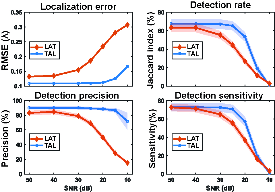
Figure 3: Noise localization and detection robustness. The four different metrics are presented for the standard concentration (C=1 a.u.). The statistical measures are computed across different numbers of buffers and shown as mean values with their respective standard deviations.

3.2 In Silico tracking performance of TAL

Figure 4 presents the tracking performance globally and locally of both methods via the velocity estimation for different concentrations. All the simulated MB trajectories were derived to obtain MB velocities. Those velocities were averaged at the positions of the associated MB to form the ground truth velocity map (Fig. 4a).

The global performance of the tracking is reflected by the correlation coefficient between the ground truth velocity map and the velocity maps obtained from the tracking of each method (Fig. 4b). At the standard concentration (C=1 a.u.), TAL achieved a correlation rate of 93%, whereas LAT achieved 79%. Similarly, at 5 times the standard concentration (C=5 a.u.), TAL achieved a correlation rate of 78%, which is comparable to LAT at the standard concentration (C=1 a.u.). Both methods exhibited a degradation in the velocity estimators as the concentration increased.

Locally, velocity profiles orthogonal to the flux in two distinct areas of the image were extracted (Fig 4.c). Those two profiles are indicated by the pink and green lines in Fig. 4.a. In the pink profiles, where both methods must estimate high velocities in large vessels, TAL demonstrated a closer estimation of the velocity than LAT and a higher robustness in the estimation for the different concentrations, although the estimator was degraded as the concentration increased. We can notice a bias for the velocity positions of the vessels obtained with LAT. In the green profiles, where low velocities in a small vessel are estimated, TAL provided a better estimation of velocity at the standard concentration (C=1 a.u.). As concentration increased, both methods exhibited less accuracy, but TAL appeared to be more consistent than LAT.

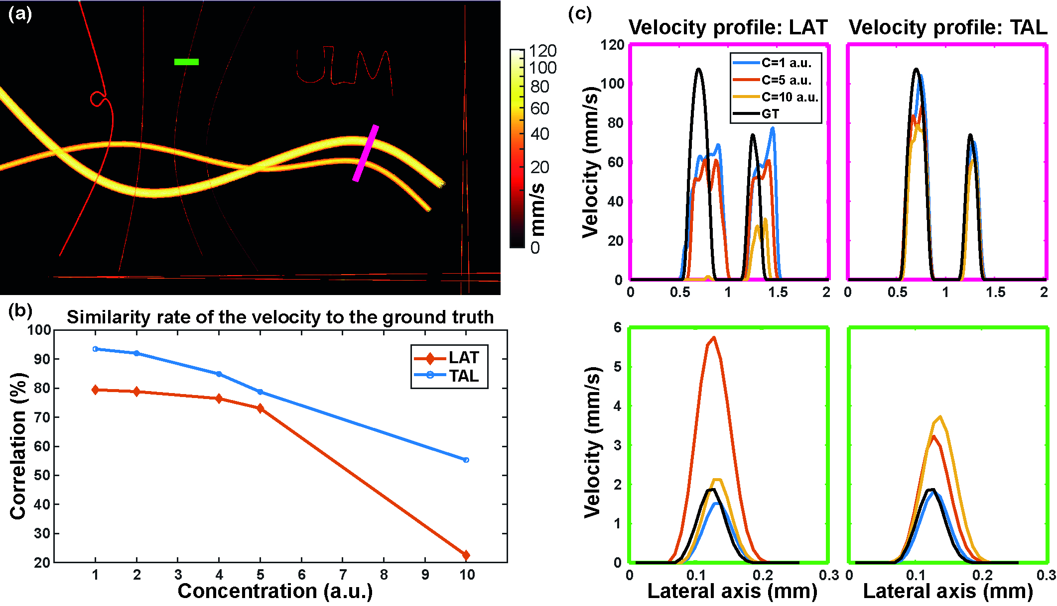
Figure 4: In Silico performances of the velocity estimator at different concentrations. (a) Ground truth velocity map resulting of the accumulation of the velocity at the positions of the MBs in 20,000 frames divided into 20 buffers initially. (b) Correlation coefficient between the ground truth velocity map and the velocity maps obtained from each approach. (c) Velocity profiles along two different lines for LAT and TAL workflow, each line taken orthogonal to the vessels to visualize the Poiseuille velocity profiles modeled in this simulation. (d) Superposed velocity profiles of the ground truth and both methods for different concentrations.

3.3 In vivo performance of TAL for ULM

Figure 5 displays the different density maps obtained for various concentrations using both methods ($C\in[1,5,10]$ a.u., see Fig. 5a) and closeup patches as well as normalized intensity profiles (Fig. 5b). The first row illustrates the density maps obtained with the LAT workflow, while the second row presents the density maps obtained with the TAL workflow.

Table 2: In vivo resolution performance (FRC) of ULM angiogram reconstruction at different concentrations for LAT and TAL workflows

Method	C=1a.u.	C=2a.u.	C=5a.u.	C=10a.u.
LAT	18.9 $\mu m$	24.4 $\mu m$	28.6 $\mu m$	30.3 $\mu m$
TAL	18.9 $\mu m$	20.4 $\mu m$	25.0 $\mu m$	27.0 $\mu m$

Qualitatively, there was a similarity between the two methods for the standard concentration, even if we notice some regions (pointed with the white arrows) where TAL recovered more details. However, as the concentration increased, both methods detected less vessels, but TAL still detected more than LAT, as illustrated by the white arrows. Moreover, as the concentration increased, both the number and length of detected vessels decreased

The associated FRC for each approach, at different concentrations, was also calculated (see Table II). At the standard concentration, both methods exhibited a similar resolution of 18.9 $\mu m$. As the concentration increased, the resolution decreased for both approaches. TAL maintained an incrementally better robustness to resolution - e.g., at a five-fold increase in concentration, TAL and LAT achieved a 25-$\mu$m and 28.6-$\mu$m resolutions, respectively.

From the normalized density profiles extracted along the white doted lines in the zoom-in regions in the cortex (Fig. 5b), we can see that for the two lowest concentrations, the differences in intensity between the vessels and the background are larger for TAL . The different values of FWHM for the main vessels are superposed to the graphs. At the standard concentration, TAL yielded a larger number of vessels and smaller diameters, indicating a better resolution. Both methods showed robustness to MB concentration in this region, as the number of vessels detected is similar, even if the size of the different vessels are changing with the concentration.

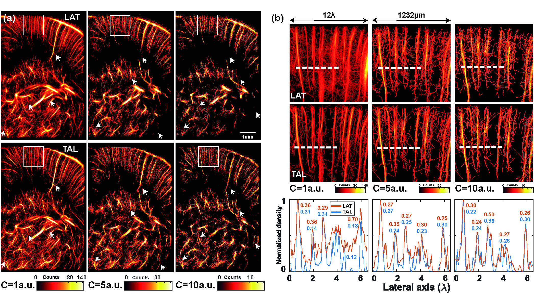
Figure 5: Impact of concentration on the vessel rendering in vivo. (a) First row presents the different density maps obtained with the standard approach (LAT pipeline), while the second presents the density maps obtained with the proposed method (TAL). Each density map is compressed with a cubic rate and saturated with a factor 0.5 relative to the maximum intensity. (b) Zoom-in of ULM angiograms on the cortex region (white square in Fig. 5a) at different concentrations for both approaches in the first two rows. The third row shows the normalized intensity profiles along a given horizontal lines overlaid by the white dotted line with corresponding vessel diameters estimated as the FWHM in wavelength

3.4 In vivo performance of TAL for DULM

3.4.1 Performance at different concentration

Figure 6 presents qualitative differences in the left hemisphere signed density maps of a rat brain for concentrations of 12.5 $\mu$L and 50 $\mu$L obtained using TAL (Fig. 6a). Quantitative differences are depicted when velocity extraction is performed over time for representative vessels using both approaches at concentrations of 12.5 $\mu$L, 25 $\mu$L and 50 $\mu$L (Fig. 6b). Qualitatively, some vessels showed differences in radius between concentrations, as exemplified by the vessel pointed out by the red arrow. At depth, both small and big vessels as well as connections between vessels were lost at high concentration. The arrows point to vessels where the velocity profiles along two cardiac cycles have been extracted in the Fig. 6b. A difference in velocity amplitude can be noticed between both methods; for instance, TAL can detect a pulsatile flow, with two clear local maxima waveform patterns, where they are expected , in all three vessels while it is less clear in the case of LAT

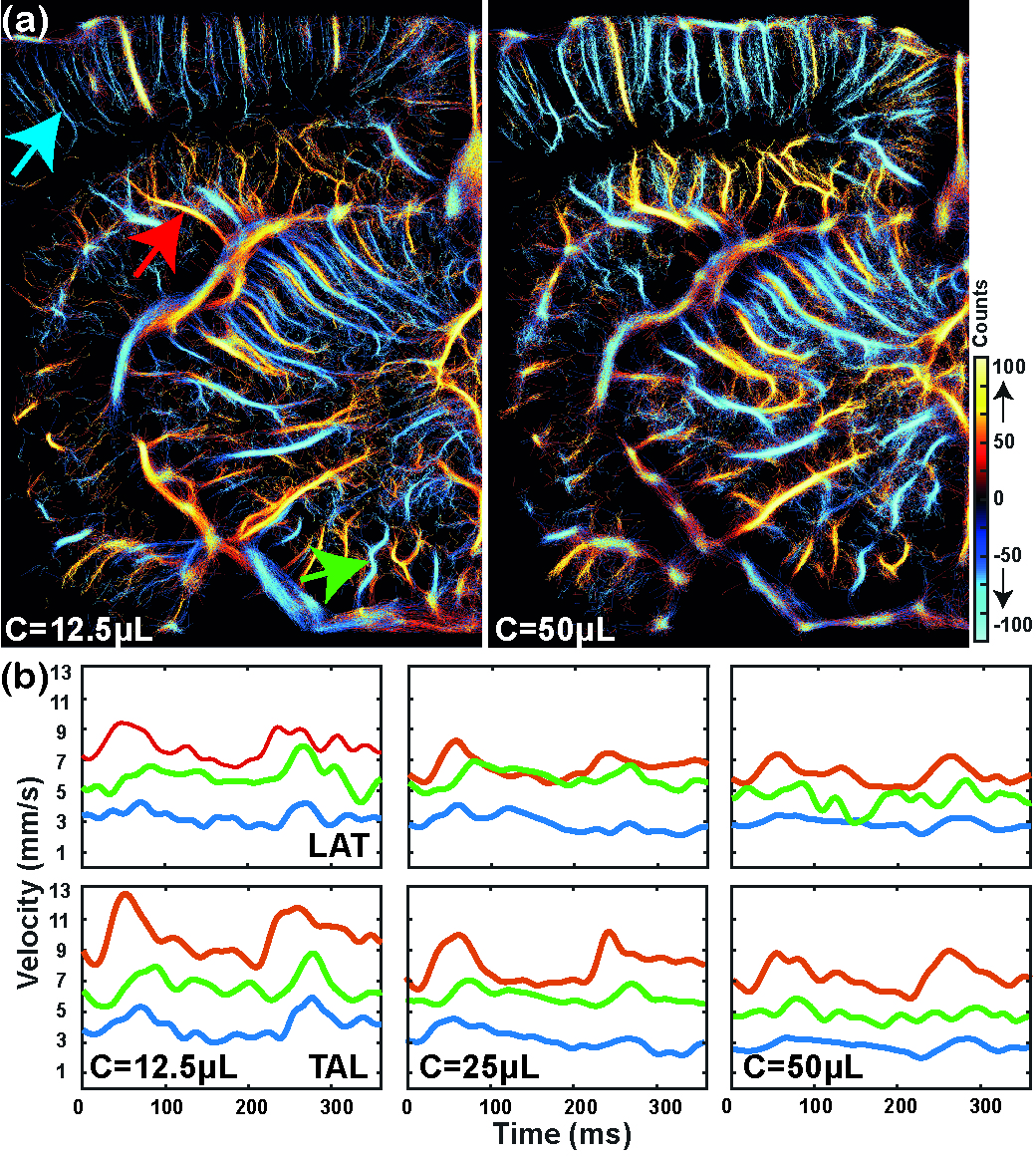
Figure 6: Velocity estimator comparison for DULM application in vivo at different concentrations in a rat brain. (a) Signed ULM maps in a rat brain for two different concentrations of microbubble (C=12.5$\mu$L and C=50$\mu$L) obtained with the TAL pipeline. (b) Velocity profiles for different vessels overlaid by different colored arrows (blue, red, and green) from the lowest concentration to the highest one (left to right) (12.5$\mu$L-25$\mu$L-50$\mu$L) obtained with the LAT & TAL methods.

3.4.2 Intra-amimal comparaison

Figure 7 shows a signed ULM reconstruction in a mouse brain using the proposed methods, with vessels highlighted by yellow, blue, red, and green arrows (Fig. 7a). These vessels’ velocities over 5 complete cardiac cycles were extracted as shown in Fig. 7b for both methods. For analysis, those vessels correspond to pairs of symmetrical vessels between the hemispheres. It is observed that the mean velocity in both hemispheres is similar (solid line for the left hemisphere and dotted line for the right one) for both methods, but TAL exhibits more consistent and synchronized fluctuations during diastole and systole events (Fig. 7b).

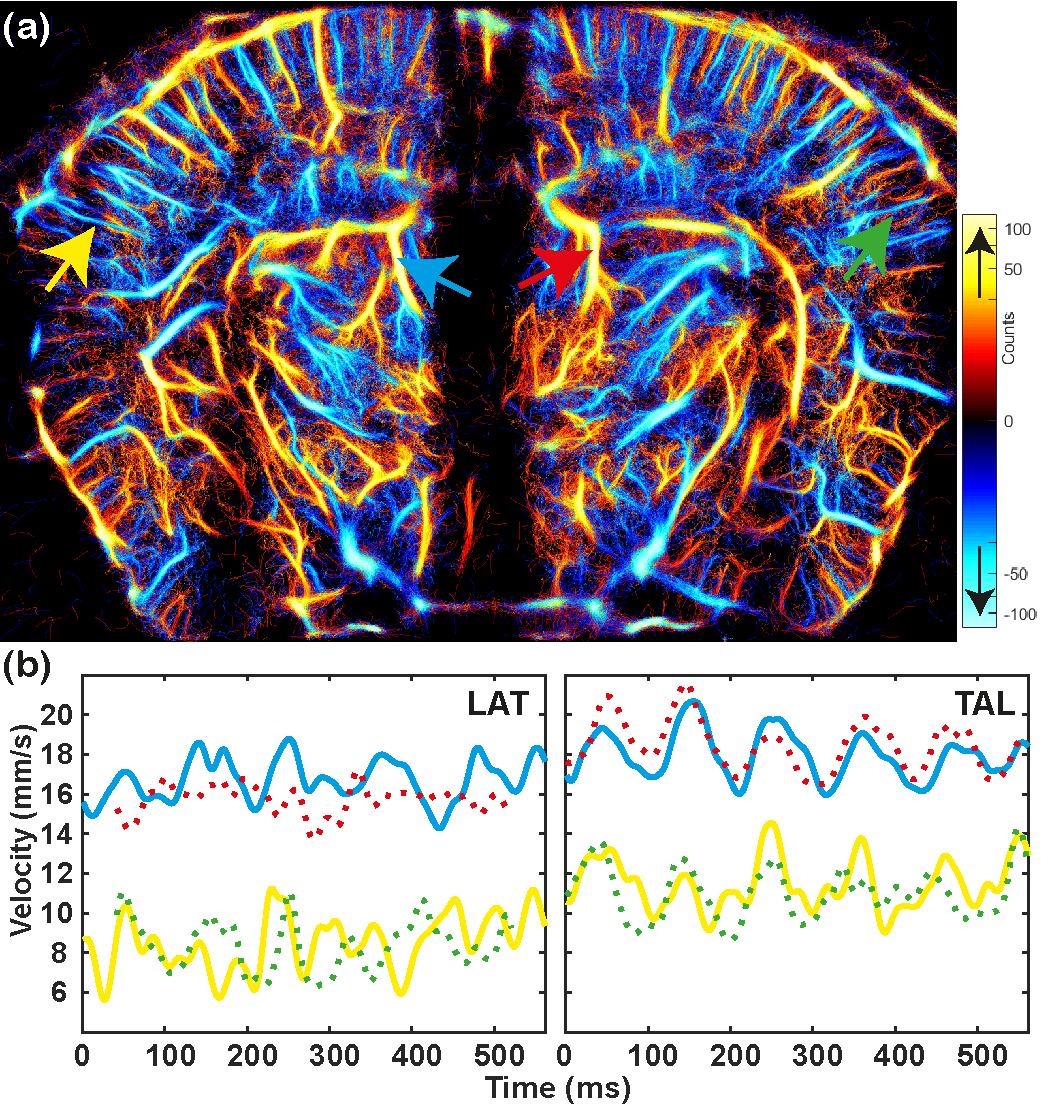
Figure 7: Hemodynamics coherence between left and right hemisphere in a mouse brain . (a) Signed Ultrasound Localization Microscopy map of a mouse brain obtained with the TAL pipeline. (b) Comparison between left and right hemisphere (solid lines: left hemisphere, dotted lines: right hemisphere) of velocity profiles for different sizes of vessels obtained with the LAT and TAL methods.

4 DISCUSSION

In this study, we introduced a processing approach that tracks prior to localizing the MB in ULM and DULM. The idea is related to the confirmation in a previous study of the hypothesis that the space-time ULM datasets carry richer information about the underlying microvascular network than individual ultrasound frames taken independently [24].

Specifically, we aimed to address the challenge of finding and tracking a larger number of MB in high concentration environments. To do so, we sought to replace the tracking part with a physically motivated pairing approach that considers global information from all frames in a buffer, rather than relying on frame-to-frame pairing based on minimal distance between localizations in adjacent frames. The choice of a tracking approach is particularly important, as recent publications in the field emphasize studying in vivo velocity to extract biomarkers [4, 5, 9, 10, 12, 45]. However, velocity estimation relies on the derivative of the trajectories, making it essential to have an accurate tracker in addition to an efficient space detection and localization algorithm to accurately estimate local blood flow. To demonstrate these objectives, we benchmarked the TAL method against the state-of-the-art LAT pipeline, both in silico and in vivo.

In the in silico experiments, we demonstrated that TAL yields superior reconstruction maps using four metrics at any concentration multiplier ranging from 1 to 10 (see Fig. 2.c). Specifically, we showed that at twice the concentration, TAL outperformed the LAT workflow at standard concentration. These results align with our first objective, as TAL allows for a twofold increase in concentration, potentially reducing acquisition time while outperforming the standard method. Additionally, we observed that TAL exhibits robustness to increased noise levels, as evidenced by its performance across varying SNR levels in silico (see Fig. 3). This robustness contributes to the reproducibility of results between experiments, where SNR can significantly vary due to experimental factors. By studying velocity in silico, we revealed the biases that arise in velocity estimators based on the chosen method and varying concentrations (see Fig. 4). TAL showed better efficiency in tracking MB and extracting accurate blood flow velocity.

To further validate our findings, we conducted in vivo validation using an open-source rat dataset and demonstrated that TAL is more robust to increasing concentration with associated reduction of acquisition times (see Fig. 5a) and maintains better resolution in the FRC study (see Table II). Density profiles also confirmed better resolved vessels in the cortex (see Fig. 5b). Indeed, at lower concentrations, the background intensity between vessels is lower with TAL, reflecting its ability to highlight more likely MB trajectories. In fact, TAL only enhances positions that are susceptible to belong to a trajectory, while LAT enhances all the positions that are likely to be a MB in space . We also successfully applied TAL to different animal models, including rats and mice.

We applied LAT and TAL to DULM and observed consistent velocity estimations across different acquisitions and concentrations within the same animal for both methods (see Fig. 6 and 7). In DULM, the TAL approach seems to extract a better pulsatile blood flow along the cardiac cycle. Between the three rat datasets, the blood flow differences observed could be attributed to the increasing concentration biasing the tracking process as illustrated in silico. It could also be attributed to physiological changes in heart beating caused by prolonged anesthesia, as the datasets were acquired successively. Additionally, at high concentrations, we recovered larger vessels that may exhibit a more efficient mapping of the range of velocities, from higher velocities in the center to lower velocities near the vessel edges, potentially explaining the overall decrease in velocity. We also demonstrated the coherence of both methods in estimating mean velocities by comparing symmetrical vessels in both hemispheres of a mouse (see Fig. 7). TAL results seem to indicate more accurate velocity variations caused by the heartbeat of the animal. The cubic smoothing spline ensures the continuity on velocity and acceleration compared to the linear interpolation. In addition, the choice of a cut-off frequency leads to a better control over the smoothing.

It is however important to acknowledge certain limitations. First, in the in vivo experiments, the ground truth for microvessels structure and blood flow velocity remain unknown. To validate our angiography and velocity estimation, it would be necessary to compare it with another imaging technique that can obtain similar spatial and temporal resolution, such as optical coherence tomography at superficial depth (1 or 2 mm). Second, while we highlighted issues with velocity estimations caused by the tracking algorithm in silico, the simulations were far from considering the complexity of a brain vasculature. Realistic simulations of brain vasculature could point out other and more specific issues [22].

From a processing perspective, the proposed method offers several advantages. First, it requires only three parameters to set, $\tau$ ,$\epsilon$ and the length of the tracks $N_{f}$ (see Table I). Note that all these parameters were very similar between the different experiments. Additionally, the calculation of the Jerman function for all voxels, which is the most computationally expensive operation (due to eigenvalues’ extractions), depends on the volume size. The thinning algorithm, responsible for providing trajectory segmentation, is a real-time algorithm. Consequently, the computational cost of the tracking part does not depend on the number of MB to pair, unlike Hungarian or graph-based algorithms.

Overall, the introduction of TAL as a novel approach addresses the challenges of tracking MB in high concentration environment and provides a physically motivated pairing strategy that considers the global continuity information available in a buffer. The method demonstrates superior performance in reconstructing hemodynamics, exhibiting robustness to noise variations, and enabling accurate velocity estimations.

These findings, supported by in silico and in vivo experiments, contribute to the advancement of subwavelength hemodynamics imaging techniques

5 CONCLUSION

We demonstrated the feasibility of recovering ULM density maps and extracting blood velocities in a range of vessels using a novel approach that reverses the localization and tracking steps. The newly proposed Tracking and Localization workflow presents a promising solution to enhance the reliability and accuracy of anatomic and functional results obtained through ULM and DULM techniques.

References

- [1] M. A. O’Reilly and K. Hynynen, “A super-resolution ultrasound method for brain vascular mapping,” Medical Physics, vol. 40, no. 11, p. 110701, 2013. _eprint: https://onlinelibrary.wiley.com/doi/pdf/10.1118/1.4823762.
- [2] C. Errico, J. Pierre, S. Pezet, Y. Desailly, Z. Lenkei, O. Couture, and M. Tanter, “Ultrafast ultrasound localization microscopy for deep super-resolution vascular imaging,” Nature, vol. 527, pp. 499–502, Nov. 2015. Number: 7579 Publisher: Nature Publishing Group.
- [3] O. M. Viessmann, R. J. Eckersley, K. Christensen-Jeffries, M. X. Tang, and C. Dunsby, “Acoustic super-resolution with ultrasound and microbubbles,” Physics in Medicine & Biology, vol. 58, p. 6447, Sept. 2013. Publisher: IOP Publishing.
- [4] M. Wiersma, B. Heiles, D. Kalisvaart, D. Maresca, and C. S. Smith, “Retrieving Pulsatility in Ultrasound Localization Microscopy,” IEEE Open Journal of Ultrasonics, Ferroelectrics, and Frequency Control, vol. 2, pp. 283–298, 2022. Conference Name: IEEE Open Journal of Ultrasonics, Ferroelectrics, and Frequency Control.
- [5] M. R. Lowerison, N. V. C. Sekaran, W. Zhang, Z. Dong, X. Chen, D. A. Llano, and P. Song, “Aging-related cerebral microvascular changes visualized using ultrasound localization microscopy in the living mouse,” Scientific Reports, vol. 12, p. 619, Jan. 2022. Number: 1 Publisher: Nature Publishing Group.
- [6] X. Chen, M. R. Lowerison, Z. Dong, N. V. C. Sekaran, D. A. Llano, and P. Song, “Localization free super-resolution microbubble velocimetry using a long short-term memory neural network,” IEEE Transactions on Medical Imaging, pp. 1–1, 2023. Conference Name: IEEE Transactions on Medical Imaging.
- [7] O. Couture, V. Hingot, B. Heiles, P. Muleki-Seya, and M. Tanter, “Ultrasound Localization Microscopy and Super-Resolution: A State of the Art,” IEEE Transactions on Ultrasonics, Ferroelectrics, and Frequency Control, vol. 65, pp. 1304–1320, Aug. 2018. Conference Name: IEEE Transactions on Ultrasonics, Ferroelectrics, and Frequency Control.
- [8] K. Christensen-Jeffries, R. J. Browning, M.-X. Tang, C. Dunsby, and R. J. Eckersley, “In Vivo Acoustic Super-Resolution and Super-Resolved Velocity Mapping Using Microbubbles,” IEEE Transactions on Medical Imaging, vol. 34, pp. 433–440, Feb. 2015. Conference Name: IEEE Transactions on Medical Imaging.
- [9] S. Dencks and G. Schmitz, “Ultrasound localization microscopy,” Zeitschrift für Medizinische Physik, June 2023.
- [10] C. Bourquin, J. Porée, F. Lesage, and J. Provost, “In Vivo Pulsatility Measurement of Cerebral Microcirculation in Rodents Using Dynamic Ultrasound Localization Microscopy,” IEEE Transactions on Medical Imaging, vol. 41, pp. 782–792, Apr. 2022. Conference Name: IEEE Transactions on Medical Imaging.
- [11] P. Cormier, J. Porée, C. Bourquin, and J. Provost, “Dynamic Myocardial Ultrasound Localization Angiography,” IEEE Transactions on Medical Imaging, vol. 40, pp. 3379–3388, Dec. 2021. Conference Name: IEEE Transactions on Medical Imaging.
- [12] N. Renaudin, C. Demené, A. Dizeux, N. Ialy-Radio, S. Pezet, and M. Tanter, “Functional ultrasound localization microscopy reveals brain-wide neurovascular activity on a microscopic scale,” Nature Methods, vol. 19, pp. 1004–1012, Aug. 2022. Number: 8 Publisher: Nature Publishing Group.
- [13] P. Song, J. M. Rubin, and M. R. Lowerison, “Super-resolution ultrasound microvascular imaging: Is it ready for clinical use?,” Zeitschrift für Medizinische Physik, May 2023.
- [14] V. Hingot, C. Errico, B. Heiles, L. Rahal, M. Tanter, and O. Couture, “Microvascular flow dictates the compromise between spatial resolution and acquisition time in Ultrasound Localization Microscopy,” Scientific Reports, vol. 9, p. 2456, Feb. 2019. Number: 1 Publisher: Nature Publishing Group.
- [15] K. Christensen-Jeffries, J. Brown, S. Harput, G. Zhang, J. Zhu, M.-X. Tang, C. Dunsby, and R. J. Eckersley, “Poisson Statistical Model of Ultrasound Super-Resolution Imaging Acquisition Time,” IEEE Transactions on Ultrasonics, Ferroelectrics, and Frequency Control, vol. 66, pp. 1246–1254, July 2019. Conference Name: IEEE Transactions on Ultrasonics, Ferroelectrics, and Frequency Control.
- [16] M. R. Lowerison, C. Huang, Y. Kim, F. Lucien, S. Chen, and P. Song, “In Vivo Confocal Imaging of Fluorescently Labelled Microbubbles: Implications for Ultrasound Localization Microscopy,” IEEE transactions on ultrasonics, ferroelectrics, and frequency control, vol. 67, pp. 1811–1819, Sept. 2020.
- [17] J. Yan, T. Zhang, J. Broughton-Venner, P. Huang, and M.-X. Tang, “Super-Resolution Ultrasound Through Sparsity-Based Deconvolution and Multi-Feature Tracking,” IEEE transactions on medical imaging, vol. 41, pp. 1938–1947, Aug. 2022.
- [18] S. Tang, P. Song, J. D. Trzasko, M. Lowerison, C. Huang, P. Gong, U.-W. Lok, A. Manduca, and S. Chen, “Kalman Filter–Based Microbubble Tracking for Robust Super-Resolution Ultrasound Microvessel Imaging,” IEEE transactions on ultrasonics, ferroelectrics, and frequency control, vol. 67, pp. 1738–1751, Sept. 2020.
- [19] P. Xing, J. Porée, B. Rauby, A. Malescot, é. Martineau, V. Perrot, R. L. Rungta, and J. Provost, “Phase Aberration Correction for in vivo Ultrasound Localization Microscopy Using a Spatiotemporal Complex-Valued Neural Network,” Feb. 2023. arXiv:2209.10650 [eess].
- [20] C. Demené, J. Robin, A. Dizeux, B. Heiles, M. Pernot, M. Tanter, and F. Perren, “Transcranial ultrafast ultrasound localization microscopy of brain vasculature in patients,” Nature Biomedical Engineering, vol. 5, pp. 219–228, Mar. 2021. Number: 3 Publisher: Nature Publishing Group.
- [21] H. Ul Banna, B. Mitchell, S. Chen, and J. Palko, “Super-Resolution Ultrasound Localization Microscopy Using High-Frequency Ultrasound to Measure Ocular Perfusion Velocity in the Rat Eye,” Bioengineering, vol. 10, p. 689, June 2023.
- [22] H. Belgharbi, J. Porée, R. Damseh, V. Perrot, L. Milecki, P. Delafontaine-Martel, F. Lesage, and J. Provost, “An Anatomically Realistic Simulation Framework for 3D Ultrasound Localization Microscopy,” IEEE Open Journal of Ultrasonics, Ferroelectrics, and Frequency Control, vol. 3, pp. 1–13, 2023. Conference Name: IEEE Open Journal of Ultrasonics, Ferroelectrics, and Frequency Control.
- [23] Y. Shin, M. R. Lowerison, Y. Wang, X. Chen, Q. You, Z. Dong, M. A. Anastasio, and P. Song, “Context-Aware Deep Learning Enables High-Efficacy Localization of High Concentration Microbubbles for Super-Resolution Ultrasound Localization Microscopy,” Apr. 2023. Pages: 2023.04.21.536599 Section: New Results.
- [24] L. Milecki, J. Porée, H. Belgharbi, C. Bourquin, R. Damseh, P. Delafontaine-Martel, F. Lesage, M. Gasse, and J. Provost, “A Deep Learning Framework for Spatiotemporal Ultrasound Localization Microscopy,” IEEE Transactions on Medical Imaging, vol. 40, pp. 1428–1437, May 2021. Conference Name: IEEE Transactions on Medical Imaging.
- [25] J. Kim, Q. Wang, S. Zhang, and S. Yoon, “Compressed Sensing-Based Super-Resolution Ultrasound Imaging for Faster Acquisition and High Quality Images,” IEEE Transactions on Biomedical Engineering, vol. 68, pp. 3317–3326, Nov. 2021. Conference Name: IEEE Transactions on Biomedical Engineering.
- [26] X. Liu, T. Zhou, M. Lu, Y. Yang, Q. He, and J. Luo, “Deep Learning for Ultrasound Localization Microscopy,” IEEE Transactions on Medical Imaging, vol. 39, pp. 3064–3078, Oct. 2020. Conference Name: IEEE Transactions on Medical Imaging.
- [27] U.-W. Lok, C. Huang, P. Gong, S. Tang, L. Yang, W. Zhang, Y. Kim, P. Korfiatis, D. J. Blezek, F. Lucien, R. Zheng, J. D. Trzasko, and S. Chen, “Fast Super-resolution Ultrasound Microvessel Imaging using Spatiotemporal Data with Deep Fully Convolutional Neural Network,” Physics in medicine and biology, vol. 66, pp. 10.1088/1361–6560/abeb31, Mar. 2021.
- [28] A. Bar-Zion, C. Tremblay-Darveau, O. Solomon, D. Adam, and Y. C. Eldar, “Fast Vascular Ultrasound Imaging With Enhanced Spatial Resolution and Background Rejection,” IEEE Transactions on Medical Imaging, vol. 36, pp. 169–180, Jan. 2017. Conference Name: IEEE Transactions on Medical Imaging.
- [29] J. Yu, L. Lavery, and K. Kim, “Super-resolution ultrasound imaging method for microvasculature in vivo with a high temporal accuracy,” Scientific Reports, vol. 8, p. 13918, Sept. 2018. Number: 1 Publisher: Nature Publishing Group.
- [30] R. J. G. van Sloun, O. Solomon, M. Bruce, Z. Z. Khaing, H. Wijkstra, Y. C. Eldar, and M. Mischi, “Super-Resolution Ultrasound Localization Microscopy Through Deep Learning,” IEEE Transactions on Medical Imaging, vol. 40, pp. 829–839, Mar. 2021. Conference Name: IEEE Transactions on Medical Imaging.
- [31] A. Bar-Zion, O. Solomon, C. Tremblay-Darveau, D. Adam, and Y. C. Eldar, “SUSHI: Sparsity-based Ultrasound Super-resolution Hemodynamic Imaging,” Sept. 2018. arXiv:1712.00648 [physics].
- [32] Q. Chen, J. Yu, B. M. Rush, S. D. Stocker, R. J. Tan, and K. Kim, “Ultrasound super-resolution imaging provides a noninvasive assessment of renal microvasculature changes during mouse acute kidney injury,” Kidney international, vol. 98, pp. 355–365, Aug. 2020.
- [33] C. Huang, M. R. Lowerison, J. D. Trzasko, A. Manduca, Y. Bresler, S. Tang, P. Gong, U.-W. Lok, P. Song, and S. Chen, “Short Acquisition Time Super-Resolution Ultrasound Microvessel Imaging via Microbubble Separation,” Scientific Reports, vol. 10, p. 6007, Apr. 2020. Number: 1 Publisher: Nature Publishing Group.
- [34] B. Heiles, A. Chavignon, V. Hingot, P. Lopez, E. Teston, and O. Couture, “Performance benchmarking of microbubble-localization algorithms for ultrasound localization microscopy,” Nature Biomedical Engineering, vol. 6, pp. 605–616, May 2022. Number: 5 Publisher: Nature Publishing Group.
- [35] G. Montaldo, M. Tanter, J. Bercoff, N. Benech, and M. Fink, “Coherent plane-wave compounding for very high frame rate ultrasonography and transient elastography,” IEEE transactions on ultrasonics, ferroelectrics, and frequency control, vol. 56, pp. 489–506, Mar. 2009.
- [36] V. Perrot, M. Polichetti, F. Varray, and D. Garcia, “So you think you can DAS? A viewpoint on delay-and-sum beamforming,” Ultrasonics, vol. 111, p. 106309, Mar. 2021.
- [37] J. Baranger, B. Arnal, F. Perren, O. Baud, M. Tanter, and C. Demené, “Adaptive Spatiotemporal SVD Clutter Filtering for Ultrafast Doppler Imaging Using Similarity of Spatial Singular Vectors,” IEEE Transactions on Medical Imaging, vol. 37, pp. 1574–1586, July 2018. Conference Name: IEEE Transactions on Medical Imaging.
- [38] C. Demené, T. Deffieux, M. Pernot, B.-F. Osmanski, V. Biran, J.-L. Gennisson, L.-A. Sieu, A. Bergel, S. Franqui, J.-M. Correas, I. Cohen, O. Baud, and M. Tanter, “Spatiotemporal Clutter Filtering of Ultrafast Ultrasound Data Highly Increases Doppler and fUltrasound Sensitivity,” IEEE Transactions on Medical Imaging, vol. 34, pp. 2271–2285, Nov. 2015. Conference Name: IEEE Transactions on Medical Imaging.
- [39] T. Jerman, F. Pernus, B. Likar, and Z. Spiclin, “Enhancement of Vascular Structures in 3D and 2D Angiographic Images,” IEEE Transactions on Medical Imaging, vol. 35, pp. 2107–2118, Sept. 2016. Conference Name: IEEE Transactions on Medical Imaging.
- [40] M. G. Wagner, “Real-time thinning algorithms for 2D and 3D images using GPU processors,” Journal of Real-Time Image Processing, vol. 17, pp. 1255–1266, Oct. 2020.
- [41] J. Porée, M. Baudet, F. Tournoux, G. Cloutier, and D. Garcia, “A Dual Tissue-Doppler Optical-Flow Method for Speckle Tracking Echocardiography at High Frame Rate,” IEEE Transactions on Medical Imaging, vol. 37, pp. 2022–2032, Sept. 2018. Conference Name: IEEE Transactions on Medical Imaging.
- [42] H. W. Kuhn, “The Hungarian method for the assignment problem,” Naval Research Logistics Quarterly, vol. 2, no. 1-2, pp. 83–97, 1955. _eprint: https://onlinelibrary.wiley.com/doi/pdf/10.1002/nav.3800020109.
- [43] V. Hingot, A. Chavignon, B. Heiles, and O. Couture, “Measuring Image Resolution in Ultrasound Localization Microscopy,” IEEE Transactions on Medical Imaging, vol. 40, pp. 3812–3819, Dec. 2021. Conference Name: IEEE Transactions on Medical Imaging.
- [44] M. van Heel and M. Schatz, “Fourier shell correlation threshold criteria,” Journal of Structural Biology, vol. 151, pp. 250–262, Sept. 2005.
- [45] K. Christensen-Jeffries, O. Couture, P. A. Dayton, Y. C. Eldar, K. Hynynen, F. Kiessling, M. O’Reilly, G. F. Pinton, G. Schmitz, M.-X. Tang, M. Tanter, and R. J. G. van Sloun, “Super-resolution Ultrasound Imaging,” Ultrasound in Medicine & Biology, vol. 46, pp. 865–891, Apr. 2020.