A Search for Technosignatures Around 11,680 Stars with the Green Bank Telescope at 1.15–1.73 GHz

Abstract

We conducted a search for narrowband radio signals over four observing sessions in 2020–2023 with the L-band receiver (1.15–1.73 GHz) of the 100 m diameter Green Bank Telescope. We pointed the telescope in the directions of 62 TESS Objects of Interest, capturing radio emissions from a total of $\sim$11,680 stars and planetary systems in the $\sim$9 arcminute beam of the telescope. All detections were either automatically rejected or visually inspected and confirmed to be of anthropogenic nature. We also quantified the end-to-end efficiency of radio SETI pipelines with a signal injection and recovery analysis. The UCLA SETI pipeline recovers $94.0\%$ of the injected signals over the usable frequency range of the receiver and $98.7\%$ of the injections when regions of dense radio frequency interference are excluded. In another pipeline that uses incoherent sums of 51 consecutive spectra, the recovery rate is $\sim$15 times smaller at $\sim$6%. The pipeline efficiency affects calculations of transmitter prevalence and SETI search volume. Accordingly, we developed an improved Drake Figure of Merit and a formalism to place upper limits on transmitter prevalence that take the pipeline efficiency and transmitter duty cycle into account. Based on our observations, we can state at the 95% confidence level that fewer than 6.6% of stars within 100 pc host a transmitter that is detectable in our search (EIRP $>$ 10¹³ W). For stars within 20,000 ly, the fraction of stars with detectable transmitters (EIRP $>$ 5 $\times$ 10¹⁶ W) is at most $3\times 10^{-4}$. Finally, we showed that the UCLA SETI pipeline natively detects the signals detected with AI techniques by Ma et al. (2023).

1 Introduction

In the 1982 decadal report, the Astronomy Survey Committee of the National Research Council (NRC) recommended the approval and funding of “An astronomical Search for Extraterrestrial Intelligence (SETI), supported at a modest level, undertaken as a long-term effort rather than as a short-term project, and open to the participation of the general scientific community” (National Research Council, 1982). The Committee noted:

It is hard to imagine a more exciting astronomical discovery or one that would have greater impact on human perceptions than the detection of extraterrestrial intelligence. After reviewing the arguments for and against SETI, the Committee has concluded that the time is ripe for initiating a modest program that might include a survey in the microwave region of the electromagnetic spectrum while maintaining an openness to support of other innovative studies as they are proposed.

In a subsequent report on the search for life’s origins, the NRC stated: “Two parallel avenues of research should be pursued in attempts to detect life beyond the solar system: searches for evidence of biological modification of an extrasolar planet and searches for evidence of extraterrestrial technology” (National Research Council, 1990). The report’s recommendations included the “commencement of a systematic ground-based search through the low end of the microwave window for evidence of signals from an extraterrestrial technology”.

The detection of extraterrestrial life forms is expected to usher profound developments in a wide range of scientific and cultural disciplines. These potential benefits provide compelling incentives to invest in multifaceted searches for biological indicators (biosignatures) and technological indicators (technosignatures) of extraterrestrial life. Searches for biosignatures and technosignatures are highly complementary. In particular, the latter can “expand the search for life in the universe from primitive to complex life and from the solar neighborhood to the entire Galaxy” (Margot et al., 2019). In the Milky Way Galaxy alone, the ratio of search volumes with current and near-future technology is $V_{\rm techno}/V_{\rm bio}\gtrsim 10^{6}$. In terms of the number of accessible targets, the ratio is $N_{\rm techno}/N_{\rm bio}\gtrsim 10^{9}$.

Although some types of solar system biosignatures (e.g., a fossil or sample organism) may offer compelling interpretations, the proposed exoplanet biosignatures are expected to yield inconclusive interpretations for some time (e.g., Fujii et al., 2018). Abiogenic interpretations may remain difficult to rule out (e.g., Rein et al., 2014), as evidenced by biosignature claims for planets that are a million times closer than the nearest exoplanet (methane on Mars, phosphine on Venus). In many cases, the spectroscopic observations may be consistent with but not diagnostic of the presence of life (e.g., Catling et al., 2018; Meadows et al., 2022). In contrast, the search for technosignatures provides an opportunity to obtain robust detections with unambiguous interpretations. An example of such a technosignature is a narrowband (say, $<$10 Hz at gigahertz frequencies) signal from an emitter located beyond the solar system. Detection of a signal with these characteristics would provide sufficient evidence for the existence of another civilization because natural settings cannot generate such signals. In order to confine the signal bandwidth within 10 Hz at L band, the velocity dispersion and Doppler broadening of the species participating in the emission must remain below 2 m/s. Such coherence in velocity would have to be maintained over the physical scales of the emission sites. Fluid astrophysical settings cannot produce such conditions because the thermal velocity of species is much larger, even in the coldest environments. Even astrophysical masers cannot maintain this degree of coherence: the narrowest reported OH (1612 MHz) maser line width is 550 Hz (Cohen et al., 1987; Qiao et al., 2020), roughly two orders of magnitude wider than the proposed narrowband radio technosignatures.

Here, we describe a search for narrowband radio technosignatures around $\sim$11,680 stars and their planetary systems. For the historical context of the search, see, e.g., Tarter (2001); Tarter et al. (2010); Technosignatures Workshop Participants (2018).

2 Observations

We observed $\sim$11,680 stars and their planetary systems in 62 distinct directions aligned with TESS Objects of Interest (TOIs). The characteristics of our primary targets are listed in Appendix A (Tables 5 and 6). To compute the number of stars captured by the 8.4 arcmin beamwidth of the telescope at 1.42 GHz, we followed Wlodarczyk-Sroka et al. (2020) and performed cone searches with the Gaia catalog (Gaia Collaboration, 2023). We found 11,680 known stars, of which 10,378 have improved geometric distance measurements calculated by Bailer-Jones et al. (2021). The median, mean, and maximum distance estimates for these sources are 2288 pc (7461 ly), 2450 pc (7990 ly), and 12,664 pc (41,305 ly), respectively. There are 10,230 sources located within 6132 pc (20,000 ly) of the Sun.

We observed these stars and their planetary systems with the Green Bank Telescope (GBT) during 2 hr sessions on 2020 April 22, 2021 April 28, 2022 May 22, and 2023 May 13. The observing cadence consisted of two scans of 150 s each per primary target, with sources arranged in pairs resulting in an A-B-A-B sequence for sources A and B. Angular separations between sources always exceeded several telescope beamwidths. These ON-OFF-ON-OFF (or OFF-ON-OFF-ON) sequences are particularly useful in the detection of radio frequency interference (RFI) (Section 3.4).

We recorded both linear polarizations of the L-band receiver with the VEGAS backend in its baseband recording mode (Anish Roshi et al., 2012). We sampled 800 MHz of bandwidth between 1.1 and 1.9 GHz. We sampled complex (in-phase and quadrature) voltages with 8-bit quantization, but preserved only 2-bit samples after requantization with an optimal four-level sampler, which yields a quantization efficiency $\eta_{Q}$ of 0.8825 (Kogan, 1998).

3 Methods

Our data processing techniques are generally similar to those used by Margot et al. (2018), Pinchuk et al. (2019), and Margot et al. (2021). Here, we give a brief overview and refer the reader to these other works for additional details.

3.1 Bandpass Correction

The VEGAS instrument splits the 800 MHz recorded bandwidth into 256 coarse channels of 3.125 MHz each. In the process of doing so, it applies a bandpass filter to each coarse channel. This filter reduces the amplitude of the baseline near both edges of the spectra. We restored an approximately flat baseline by dividing each spectrum by a model of the bandpass filter response. This model was obtained by fitting a 16-degree Chebyshev polynomial to the median bandpass response of 28 scans in the 1664.0625–1667.1875 MHz frequency range, which is generally devoid of interference because it falls in the middle of the radio astronomy protected band (1660.6–1670.0 MHz) for the hydroxyl radical. We enforced an even response by setting the odd coefficients of the polynomial to zero.

3.2 Doppler Dechirping

Over the 150 s duration of our scans, narrowband signals from fixed-frequency transmitters are well approximated at the receiver by linear frequency modulated (FM) “chirp” signals, where the rate of change in frequency is dictated by the orbital and rotational motions of both the emitter and the receiver. The linear FM waveform is characterized by a signal of the form

$$s(t)=A\cos(2\pi(f_{0}t+Kt^{2}/2)),\hskip 56.9055pt0\leq t\leq\tau,$$ (1)

where $A$ is the signal amplitude, $f_{0}$ is the frequency at $t=0$, $K$ is the rate of change of the frequency, and $\tau$ is the duration of the scan. In complex exponential notation,

$$s(t)=A\exp{(j2\pi(f_{0}t+Kt^{2}/2))}=A\exp{(j\theta(t))},\hskip 56.9055pt0\leq t\leq\tau.$$ (2)

The instantaneous frequency is the time derivative of the phase, i.e.,

$$f(t)=\frac{1}{2\pi}\frac{d\theta(t)}{dt}=f_{0}+Kt.$$ (3)

The frequency increases linearly as $f(t)=f_{0}+Kt$, with a total frequency excursion equal to $K\tau$. An audible signal with this time-frequency behavior would sound like a chirp, hence the name commonly attributed to the waveform.

Doppler dechirping consists of compensating for a signal’s drift in time-frequency space to facilitate integration of the signal power over the scan duration. In SETI searches, the drift rate is not known a priori. We used a tree algorithm of complexity O($N\log N$) (Taylor, 1974; Siemion et al., 2013) to integrate the signal power at 1023 trial drift rates over the range $\pm 8.86$ Hz s^-1 with a drift rate resolution of $\Delta\dot{f}=0.0173$ Hz s^-1. This approximate technique, known as incoherent dechirping, does not recover 100% of the signal power. Margot et al. (2021) quantified this signal loss with a dechirping efficiency factor $\eta_{D}$ $(0\leq\eta_{D}\leq 1)$ for a variety of settings, including searches that utilize incoherent summing of power spectra prior to signal detection. In this and previous UCLA SETI work, we do not use incoherent averaging (i.e., $N_{\rm INC\_SUMS}=1$) and the dechirping efficiency ranges between 60% and 100% with an average $\eta_{D}\simeq 72\%$ over the $\pm 8.86$ Hz s^-1 drift rate range. For searches with $N_{\rm INC\_SUMS}=51$ over a $\pm 4$ Hz s^-1 drift rate range (e.g., Price et al., 2020; Gajjar et al., 2021) the dechirping efficiency ranges between 4% and 100% with an average $\eta_{D}\simeq 16\%$. Importantly, the nominal performance of the tree algorithm for such searches is maintained in only a fairly narrow range of drift rates up to $\pm 0.15$ Hz s^-1, and the efficiency drops precipitously at larger drift rates due to Doppler smearing of the signal (Margot et al., 2021, Figure 7).

The received frequency $f_{r}$ of a monochromatic transmission at frequency $f_{t}$ experiences a time rate of change that depends on the line-of-sight acceleration $\dot{v}$ between transmitter and receiver. To first order,

$$\frac{\dot{f}_{r}}{f_{t}}=\frac{\dot{v}}{c},$$ (4)

where the overdot denotes a time derivative and $c$ is the speed of light. Our selection of a range of trial drift rates with maximum value $\dot{f}_{r,\rm max}=\pm 8.86$ Hz s^-1 corresponds to a fractional drift rate of $\pm$6.24 nHz at $f_{t}$ = 1.42 GHz (maximum accelerations $\dot{v}_{\rm max}$ of 1.87 ms^-2). It is an appropriate choice because it accommodates line-of-sight accelerations due to the spins and orbits of most exoplanets. It can handle accelerations due the orbits of $\sim$73% of confirmed exoplanets with known semi-major axes and orbital periods, $\sim$93% of confirmed exoplanets with semi-major axes greater than 0.05 au, and 100% of confirmed exoplanets with semi-major axes greater than 0.1 au (NASA Exoplanet Archive, 2019). It can also handle accelerations due to the spins of Earth-size planets at arbitrary periods (above the rotational breakup period) and Jupiter-size planets with spin periods greater than 11.5 hr. Transmitters located on exotic platforms that somehow exceed these limits could escape detection by our pipeline if the transmitted waveforms were not compensated to account for the platform’s acceleration (Figure 1).

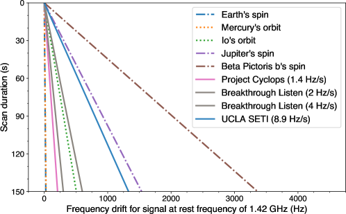
Figure 1: Expected frequency drifts from monochromatic ($f_{t}$ = 1.42 GHz) transmitters experiencing spin and orbital accelerations in various settings. The solid lines represent the maximum drift rates corresponding to Project Cyclops, Breakthrough Listen (BL), and UCLA SETI searches. This figure is adapted from Sheikh et al. (2019) and reduces the drift rates sampled by BL by a factor of $\sim$7 to correct an error in the original figure.

3.3 Signal Detection

At each frequency bin, our algorithm selects the trial drift rate that yields the greatest integrated signal power and determines whether the prominence of the signal (Margot et al., 2021) exceeds 10 times the standard deviation of the noise. The properties of signals that exceed the threshold are stored in a structured query language (SQL) database.

In practice, the algorithm proceeds in order of decreasing prominence in each coarse channel.

3.4 Doppler and Direction-of-origin Filters

Signals with $\dot{f}_{r}=0$ are marked as anthropogenic RFI because they imply zero line-of-sight acceleration between the transmitter and receiver. Signals that are detected in more than one direction on the sky are also marked as RFI because a signal emitted beyond the solar system can appear in only one telescope beam. Finally, sources that are detected in only one of the two scans are also marked as intermittent RFI.

The direction-of-origin filter, also known as a directional filter or sky localization filter, can be run efficiently by retrieving the signal properties from our SQL database. A more stringent filter can be obtained by running the machine-learning (ML) algorithm of Pinchuk & Margot (2022).

3.5 Visual Inspection of the Remaining Signals

Signals that remain after the line-of-sight distance and acceleration elimination process are marked as candidate technosignatures. All such candidates that fall outside of permanent RFI bands (Pinchuk et al., 2019) are visually inspected.

3.6 Sensitivity

The flux from a transmitter with equivalent isotropic radiated power (EIRP) at distance $r$ is $S={\rm EIRP}/(4\pi r^{2}).$

The signal-to-noise ratio (S/N) of a narrowband radio link has been computed by, e.g., Friis (1946); Kraus (1986); Enriquez et al. (2017); Margot et al. (2018). It reads

$$S/N=\frac{S}{\rm SEFD}\sqrt{\frac{n_{\rm pol}\tau}{\Delta f}},$$ (5)

where $S$ is the observed flux, SEFD is the system equivalent flux density, a common measure of telescope and receiver performance, $n_{\rm pol}$ is the number of polarizations summed incoherently, $\tau$ is the integration time, and $\Delta f$ is the channel receiver bandwidth (i.e., frequency resolution).

In a more rigorous formulation, the S/N includes the quantization efficiency $\eta_{Q}$ due to imperfect digitization of the voltage signals and the dechirping efficiency $\eta_{D}$ due to imperfect integration of the signal power (Margot et al., 2021):

$$S/N=\eta_{Q}\eta_{D}\frac{S}{\rm SEFD}\sqrt{\frac{n_{\rm pol}\tau}{\Delta f}}.$$ (6)

Quantization efficiency approaches unity with 8-bit sampling and is $\eta_{Q}$ = 88.25% for an optimal 2-bit sampler (Kogan, 1998). Dechirping efficiency with an O($N\log N$) algorithm depends on the frequency drift rate and ranges between 60% and 100% for the data acquisition and processing choices in this and previous UCLA SETI work, and between 4% and 100% for a BL-like process with $N_{\rm INC\_SUMS}=51$ and $\dot{f}_{r}$ within $\pm$4 Hz s^-1. It is possible to improve the dechirping efficiency if one is willing to use a costly O($N^{2}$) incoherent dechirping algorithm. For signals of interest with known frequency drift rates, UCLA SETI has the capability to apply a coherent dechirping algorithm to the raw voltage data, in which case $\eta_{D}\simeq 1$.

For the UCLA SETI program at the GBT, we have $\eta_{Q}$ = 0.8825, SEFD = 10 Jy, $n_{\rm pol}$ = 2, $\tau$ = 150 s, and $\Delta f$ $\simeq$ 3 Hz. Our usual detection threshold is set at S/N=10, such that signals with flux $S_{\rm det}=11.3\times 10^{-26}$ W/m² are detectable. With these parameters, an Arecibo Planetary Radar (EIRP=$2.2\times 10^{13}$ W) is detectable at 415 ly and a thousand Arecibos can be detected at 13,123 ly. Conversely, transmitters located 326 ly (100 pc) away are detectable with 0.62 Arecibos (EIRP=$1.35\times 10^{13}$ W), transmitters located 20,000 ly (6132 pc) away are detectable with 2323 Arecibos (EIRP=$5.08\times 10^{16}$ W), and transmitters located at the galactic center are detectable with 4130 Arecibos.

3.7 Signal Injection and Recovery Analysis

To quantify the end-to-end efficiency of the UCLA SETI pipeline, we injected 10,000 artificial chirp signals in raw voltage data from our 2021 search, processed the data as we normally do, and quantified the number of injected signals that were recovered by the pipeline.

We used Equation (2) to inject the artificial signals in complex voltage data sampled with 8 bit quantization, and we adjusted the signal amplitudes to achieve an S/N upon recovery of approximately 20. The starting frequencies of the signals were drawn randomly from a uniform distribution in the range 1.15–1.73 GHz, with the exclusion of the 1.20–1.34 GHz range that is blocked by a notch filter at the GBT. The drift rates were drawn randomly from a uniform distribution in the range $\pm 8.86$ Hz s^-1 (Figure 2).

We used the exact same data files (raw voltage data files injected with 10,000 artificial signals) to estimate the end-to-end efficiency of a process that imitates the Breakthrough Listen (BL) pipeline. Specifically, we computed power spectra with the FFTW library (Frigo & Johnson, 2005) and a transform length of $2^{20}$, yielding a frequency resolution $\Delta f=2.98$ Hz that approximates the finest frequency resolutions (2.79 Hz, 2.84 Hz, 2.93 Hz) of BL spectra  (Lebofsky et al., 2019, Table 4). We applied a bandpass correction appropriate for the BL data acquisition backend. We then summed 51 consecutive power spectra incoherently, yielding a time resolution of 17.11 s, to approximate the 51-fold incoherent summing and time resolutions (17.40 s, 17.98 s, 18.25 s) of the High Spectral Resolution (HSR) BL spectra (Lebofsky et al., 2019, Table 4). Finally, we ran BL’s version of the Doppler dechirping tree algorithm, as implemented in turboSETI (Enriquez et al., 2017), with a maximum drift rate of $\pm 8.88$ Hz s^-1 and minimum S/N of 10, to identify signals and quantify the number of injected signals that were recovered (turboSETI -M 8.881784197 -s 10).

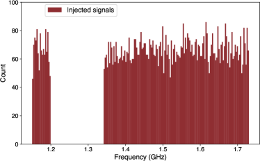
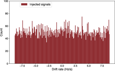
Figure 2: Distributions of starting frequencies (Left) and drift rates (Right) of 10,000 artificial, linear FM “chirp” signals injected in voltage data. Frequencies corresponding to a notch filter at the GBT (1.2 – 1.3412 GHz) are excluded.

A signal was deemed to be recovered if two conditions were jointly met: (1) the recovered frequency was within $\pm$6 Hz of the injected frequency, and (2) the recovered drift rate was within $\pm$0.05 Hz s^-1 of the injected drift rate. These tolerances were designed to accommodate slight mismatches of up to two bins in the frequency dimension and the frequency drift rate dimension. The probability of an accidental match is less than one in a billion. Because of differences in algorithm implementation, the drift rate bins were 0.0173 Hz s^-1 for UCLA SETI and 0.0249 Hz s^-1 for turboSETI.

3.8 Native Detections of ML Candidates by the UCLA SETI Pipeline

Ma et al. (2023) used a $\beta$-convolutional variational autoencoder and random forest analysis to identify eight promising signals not previously identified by the BL pipeline. They named these candidates MLc1 to MLc8, in reference to the machine learning (ML) process used in their analysis. We were interested in finding out whether these signals could be natively detected by the UCLA SETI pipeline, without any ML assistance. We downloaded the BL HSR power spectra of the MLc candidates and corresponding OFF scans, applied a bandpass correction (Section 3.1) appropriate for the BL data acquisition backend, and ran the resulting spectra through the UCLA SETI pipeline. We used only the first four of six scans of each pair of sources to mimic the A-B-A-B sequence used in UCLA SETI observations.

4 Results

4.1 Candidate Technosignatures

We detected 41.2 million narrowband signals with the data from our 2020–2023 observations. Almost all (99.43%) of these signals were rejected automatically by the UCLA SETI pipeline as RFI, which left approximately 230,000 signals warranting further consideration. Tens of thousands of these signals are being inspected by thousands of volunteers on the website http://arewealone.earth as part of a citizen science collaboration (Li & Margot, 2023). Almost all (99.78%) of the remaining signals were detected in regions of dense RFI. We visually inspected all $\sim$500 candidate technosignatures that were detected outside of dense RFI regions and determined that they were all anthropogenic.

It is remarkable that, in over 82 million narrowband signal detections obtained during an 8-year period (Table 1), not a single signal has merited follow-up observations. There have been plenty of instances where promising signals were only marginally detected in the corresponding OFF scans. We eliminate such signals from consideration.

Data Set	Fields	Targets	Stars	Signals	Hit Rate Density	DFM	MDFM
		(primary)	(in beam)	(millions)	(sig kHz-1 hr-1)	(GHz m3 W-3/2)	(Hz2 m3 W-3/2)
UCLA 2016	Kepler	14	11,658	5.22	10.2	6.74e+31	3.95e+32
UCLA 2017	Kepler+	12	6,924	8.52	16.2	6.35e+31	3.72e+32
UCLA 2018–19	Gal. plane	30	25,293	27.0	24.6	1.44e+32	8.47e+32
UCLA 2020–23	TESS	62	11,680	41.2	18.2	2.99e+32	1.75e+33
Total 2016–23		118	55,555	82.0	19.0	5.74e+32	3.37e+33

Table 1: UCLA SETI search characteristics, showing observation fields, number of primary targets, number of stars observed in the beam of the telescope, number of narrowband signals detected with S/N$>$10, hit rate density (number of detections per unit bandwidth per unit on-source time), Drake Figure of Merit (DFM), and modified DFM (Section 5.1). Properties of all 2016–2019 detections are available online (Margot et al., 2020a, c, b).

4.2 Signal Injection and Recovery Analysis

The UCLA SETI pipeline recovered 9400 signals out of 10,000 injections, yielding an end-to-end pipeline efficiency for narrowband chirp signals of 94%. When regions of dense RFI were excluded, the UCLA SETI pipeline recovered 6716 signals out of 6807 injections, for an improved recovery rate of 98.7% (Figure 3). The distributions of recovered S/Ns and drift rates match those of the injected population (Figure 4). Signals that were not recovered are usually found near the bandpass edges, where the bandpass response and correction may be less than ideal, or intersect other signals in time-frequency space.

A process designed to imitate the BL pipeline recovered a much smaller fraction of the injections. Specifically, only 570 signals out of 10,000 injections were recovered, with S/N and drift rate distributions that do not match the injected population and illuminate the reasons for the poor performance (Figure 5). Almost all (99.1%) signals recovered by the BL-like process have drift rates within $\pm 1$ Hz s^-1. Injections with larger drift rates are rarely recovered. This result is entirely consistent with the theoretical expectation of low dechirping efficiency for high drift rate signals observed in incoherently summed power spectra. In this situation, the signal power gets smeared across multiple frequency resolution cells because of Doppler drift during the longer integration times. For BL incoherent sums of 51 spectra at $\sim$3 Hz resolution, which extend the integration times from $\sim$0.3 s to $\sim$17 s, drift rates that exceed $\pm 0.15$ Hz s^-1 experience Doppler smearing. The dechirping efficiency falls rapidly, reaching 16% for drift rates of 1 Hz s^-1 (Margot et al., 2021), making recovery of signals at larger drift rates challenging. The diminishing performance as a function of drift rate is evident when plotting the S/Ns of signals recovered by the BL-like process as a function of drift rate (Figure 6).

Detailed signal counts are listed in Table 2. These counts provide reasonable estimates of the end-to-end pipeline efficiency of radio SETI pipelines. The efficiency of a BL-like process is $\sim$5.7% for drift rates within $\pm$8.88 Hz s^-1. Because injected signals have uniformly distributed drift rates and because all recovered signals have drift rates within the $\pm$4 Hz s^-1 range used by Price et al. (2020) and Gajjar et al. (2021), we can estimate the end-to-end pipeline efficiency of their searches at $5.7\%\times 8.88/4=12.7\%$. Likewise, we find $5.7\%\times 8.88/2=25.3\%$ for the work of Enriquez et al. (2017), who sampled drift rates within $\pm$2 Hz s^-1.

	Number of hits	Number of hits	Candidate	Actual	Pipeline
	prior to injection	after injection	matches	matches	efficiency
UCLA SETI pipeline	329,591	338,238	9634	9400	94.0%
BL-like process	7512	8226	714	570	5.7%

Table 2: Efficiency of radio SETI pipelines quantified by the recovery rates of 10,000 artificial signal injections. In the UCLA SETI pipeline, a hit is defined as a narrowband signal detection with S/N $\geq$ 10. In the BL pipeline, a hit has the additional requirement of a minimum distance ($\sim$ kHz) from previously recorded hits. The factor of $\sim$50 difference in number of hits between UCLA and BL for the same data set and drift rate range has been previously documented and is understood primarily as the result of differences in dechirping efficiency and definition of a hit (Margot et al., 2021). Because injected signals may replace one or more previously detected signals, the number of candidate matches after injection is not simply the difference in number of hits prior to and after injection. Actual matches are defined as having both a recovered frequency within $\pm$6 Hz of the injected frequency and a drift rate within $\pm$0.05 Hz s^-1 of the injected drift rate. Although turboSETI in its debug mode can be coerced to reveal additional hits beyond its nominal hits, the number of actual matches in debug mode remains low at 670 recoveries out of 10,000 injections.

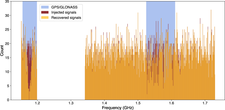
Figure 3: Distribution of injected signals and signals recovered by the UCLA SETI pipeline as a function of frequency. Blue bands indicated the operating bands of GPS and GLONASS satellites, where recovery rates are markedly lower. Frequencies corresponding to a notch filter at the GBT (1.2 – 1.3412 GHz) are excluded.

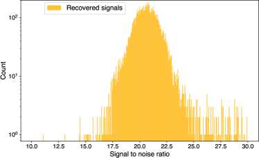
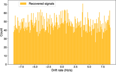
Figure 4: Distributions of the recovered S/Ns (Left) and drift rates (Right) for the UCLA SETI pipeline.

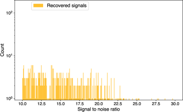
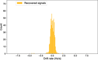
Figure 5: Distributions of the recovered S/Ns (Left) and drift rates (Right) for a process that imitates the BL pipeline, i.e., incoherent averaging of the spectra with $N_{\rm INC\_SUMS}=51$ followed by signal detection with turboSETI.

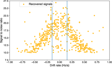
Figure 6: Distribution of the recovered S/Ns as a function of drift rate (0–1 Hz s^-1 only) for a process that imitates the BL pipeline. Only the central region within $\pm$0.15 Hz s^-1 (blue lines) is free of Doppler smearing. The recovered S/N values are lower than the injected values because of Doppler smearing that worsens at larger drift rates, as quantified by smaller dechirping efficiencies at larger drift rates. Dechirping calculations for a BL-like process had predicted a drop in S/N to about $\sim$62% of nominal for ${df}/{dt}$ = 0.25 Hz/s, $\sim$31% for ${df}/{dt}$ = 0.5 Hz/s, and $\sim$16% for ${df}/{dt}$ = 1 Hz/s (Margot et al., 2021), which is roughly consistent with what is observed.

4.3 Native Detections of Machine Learning Candidates by the UCLA SETI Pipeline

The UCLA SETI pipeline successfully detected MLc3, MLc4, MLc5, MLc7, and MLc8 without invoking our own ML algorithms (Pinchuk & Margot, 2022). We did not attempt to detect MLc1, MLc2, and MLc6 because the drift rates reported by Ma et al. (2023) for these signals (1.11 Hz s^-1, 0.44 Hz s^-1, 0.18 Hz s^-1) exceed the nominal range of the O($N\log N$) tree algorithm given the incoherent summing of 51 consecutive spectra in BL HSR data products. Based on the characteristics and appearance of the signals, we predict that if the raw voltage data had been preserved, we could have recovered MLc1, MLc2, and MLc6 by processing the data without incoherent summing.

The characteristics of the signals detected by the UCLA SETI pipeline generally match those of the ML detections well (Table 3). The magnitudes of the drift rates match, but the signs differ, which we attribute to an error in Ma et al. (2023)’s report because our values are consistent with the signal slopes in their supplemental figures.

ID	Target	Band Freq${}_{\rm\,Ma}$	Freq${}_{\rm\,UCLA}$	Offset	MJDMa	MJDUCLA	DRMa	DRUCLA	S/NMa	S/NUCLA
	(HIP)	(Hz)	(Hz)	(Hz)	(days)	(days)	(Hz s-1 )	(Hz s-1 )
MLc1	13402	1,188,539,231	N/A	N/A	57541.68902	57541.6890	+1.11	N/A	6.53	N/A
MLc2	118212	1,347,862,244	N/A	N/A	57752.78580	57752.9095	-0.44	N/A	16.38	N/A
MLc3	62207	1,351,625,410	1,351,623,638	-1772	57543.08647	57543.1000	-0.05	+0.049	57.52	80.31
MLc4	54677	1,372,987,594	1,372,984,455	-3139	57517.08789	57517.1017	-0.11	+0.11	30.20	41.71
MLc5	54677	1,376,988,694	1,376,984,409	-4285	57517.09628	57517.1017	-0.11	+0.108	44.58	63.50
MLc6	56802	1,435,940,307	N/A	N/A	57522.13197	57522.1527	-0.18	N/A	39.61	N/A
MLc7	13402	1,487,482,046	1,487,476,704	-5342	57544.51645	57544.5977	+0.10	-0.069	129.16	113.14
MLc8	62207	1,724,972,561	1,724,970,630	-1931	57543.10165	57543.1000	-0.126	+0.138	34.09	19.85

Table 3: Characteristics of the top eight signals of interest identified by Ma et al. (2023)’s ML model and corresponding detections by the UCLA SETI pipeline. MLc1, MLc2, and MLc6 have frequency drift rates beyond the nominal range of the O($N\log N$) tree algorithm and we did not attempt to detect them. Columns 3, 6, 8, and 10 with subscripts “Ma” indicate the band frequency, start epoch, frequency drift rate, and S/N as reported by Ma et al. (2023). Columns 4, 5, 7, 9, and 11 with subscripts “UCLA” are corresponding UCLA SETI results. Ma et al. (2023) did not report the frequencies of the signals but rather the center frequencies of the bands in which the signals were identified. We report the actual frequencies of the signals at the beginning of each scan (column 4) and the frequency offsets (column 5) from the band centers. The modified Julian dates (MJDs) reported by Ma et al. (2023) are erroneous except for the first one. We provided the correct values (column 7). We found frequency drift rates (DR) (column 9) that are opposite in sign to those reported by Ma et al. (2023) – our values are consistent with the signal slopes in their supplemental figures. S/N values differ because of algorithmic differences in outlier rejection when computing the standard deviation of the noise.

MLc3 was detected by the UCLA SETI pipeline but correctly identified automatically as RFI because the same signal is detected in the OFF scan at S/N$\sim$12 (Figure  7, Left).

MLc4 was detected by the UCLA SETI pipeline and identified as a candidate warranting visual inspection. Visual inspection clearly reveals the presence of the signal in the OFF scan (Figure  7, Center), indicating that this candidate is RFI.

MLc5 was detected by the UCLA SETI pipeline and identified as a candidate warranting visual inspection. Detection of the signal in the OFF scan is less compelling (Figure  7, Right), but the similarity in signal morphology with MLc4 indicates that this candidate is RFI. The frequency spacing between MLc4 and MLc5 is almost exactly 4 MHz, which suggests a common interferer.

MLc7 was detected by the UCLA SETI pipeline but correctly identified automatically as RFI because the same signal is detected in the OFF scan.

MLc8 was detected by the UCLA SETI pipeline and identified as a candidate warranting visual inspection. The signal is detected in the OFF scan and therefore labeled as RFI.

In summary, none of the MLc signals detected in our work warrant further examination.

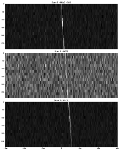
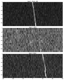
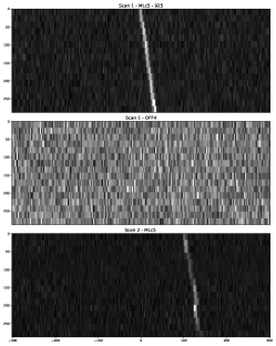
Figure 7: (Left) Dynamic spectra showing the ON-OFF-ON scans corresponding to MLc3 as detected by the UCLA SETI pipeline. The detection of the signal in the OFF scan indicates that the signal can be immediately identified as RFI. (Center) Same data for MLc4, which was identified by the UCLA SETI pipeline as a candidate worthy of visual inspection. (Right) Same data for MLc5, which was identified by the UCLA SETI pipeline as a candidate worthy of visual inspection.

5 Discussion

5.1 Figures of Merit

The Drake Figure of Merit (Drake, 1984) provides an estimate of the search volume of a SETI program that captures almost all essential elements: frequency coverage, sky coverage, and sensitivity. It is defined as

$${\rm DFM}=\frac{B\,\Omega}{S_{\rm det}^{3/2}},$$ (7)

where $B$ is the total bandwidth examined, $\Omega$ is the fractional area of the sky covered, and $S_{\rm det}$ is the minimum flux required for a detection. Typical units are GHz m³ W^-3/2 (e.g., Horowitz & Sagan, 1993).

For transmitters of a given EIRP, the $S_{\rm det}^{-3/2}$ factor is proportional to the total volume that can be examined by a search with minimum detectable flux $S_{\rm det}(\propto{\rm EIRP}/4\pi r_{\rm max}^{2})$. The fraction of this volume that is actually sampled by the search is proportional to the fraction $\Omega$ of a 4$\pi$ solid angle. Multiple observations of the same patch of sky with similar observing parameters can easily be accounted for by rewriting $\Omega=\sum_{i}\Omega_{i}$, where the index $i$ represents individual observations. As such, $\Omega$ should be viewed as an effective solid angle and not a physical solid angle. In this context, one observation is defined as a complete set of scans, e.g., two scans of source A for the UCLA SETI cadence. The fraction of the entire radio spectrum that is captured by the search is proportional to the bandwidth $B$.

In its original form, the DFM misses two essential elements. First, it assumes that pipelines are perfect with end-to-end pipeline efficiencies of 100%, whereas the efficiency of different programs can vary by more than an order of magnitude (Table 2). Second, it ignores the frequency drift rate coverage, i.e., range of line-of-sight accelerations sampled in a search, whereas this range is an obvious indicator of the thoroughness of the search. We propose a modified DFM to address these limitations:

$${\rm MDFM}=\eta_{P}\,\frac{\dot{v}_{\rm max}}{c}\frac{B\,\Omega}{S_{\rm det}^{3/2}},$$ (8)

where $\eta_{P}$ is the end-to-end pipeline efficiency for the detection of signals of interest and $\dot{v}_{\rm max}/c$ is the maximum fractional frequency drift rate (with respect to the center of the band) considered in the search (Equation 4). We express the latter in units of nHz and show MDFM values in units of Hz² m³ W^-3/2. We chose a metric that is linear in the range of frequency drift rates examined because we cannot predict the locations, sizes, or spins of preferred transmitter platforms. In the absence of reliable information, a uniform prior distribution for the frequency drift rate seems reasonable. One could design the distribution to accommodate the majority of exoplanet settings, with an upper limit of 26 nHz that accommodates 95% of confirmed exoplanets with known semi-major axes and orbital periods.

Values of the DFM and MDFM metrics for the UCLA SETI search are compared to those of select surveys in Table 4 and Figure 8. We have assumed $\eta_{P}$ = 100% for the surveys of Horowitz & Sagan (1993) and Harp et al. (2016) and the estimates of Section 4.2 for the surveys of Enriquez et al. (2017), Price et al. (2020), and UCLA SETI. The drift rate coverage of Horowitz & Sagan (1993) is unlike those of modern surveys. It is large but samples only three distinct values (local standard of rest, galactic barycenter, and cosmic microwave background rest frame). We have assumed a fractional drift rate of 1 nHz as a compromise, which is the same value that Harp et al. (2016) used. We found that the MDFM of the UCLA SETI search falls in between the survey of 692 primary stars of Enriquez et al. (2017) and the survey of 1327 primary stars of Price et al. (2020).

	Horowitz & Sagan 1993	Harp et al. 2016	Enriquez et al. 2017	Price et al. 2020	UCLA SETI
Freq. coverage $B$ (GHz)	4e-4	variablea	0.660	variableb	0.439
Sky fraction $\Omega$	0.7	1.17e-3c	2.88e-4	5.03e-4	4.91e-5
Sensitivity $S_{\rm det}$ (W/m2)	1700e-26d	260e-26e	17.7e-26f	variableg	11.3e-26h
Pipeline efficiency $\eta_{P}$	100%	100%	25.3%	12.7%	94.0%
Drift rate coverage (nHz)	1	1	1.33	2.66	6.24
DFM (GHz m3 W-3/2)	1.23e+31	1.70e+32	2.56e+33	2.59e+34	5.74e+32
MDFM (Hz2 m3 W-3/2)	1.23e+31	1.70e+32	8.63e+32	1.21e+34	3.37e+33

Table 4: Search volume characteristics of select surveys. The Drake Figure of Merit (DFM) does not account for pipeline efficiency nor frequency drift rate coverage, but the Modified Drake Figure of Merit (MDFM) does.

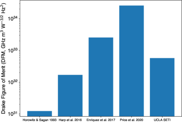
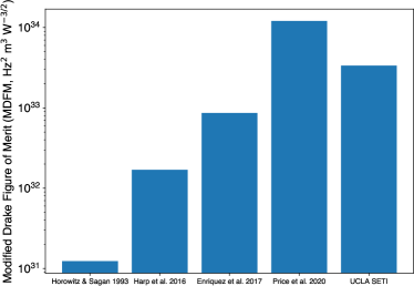
Figure 8: Search volume characteristics of select surveys. The Drake Figure of Merit (DFM, Left) does not account for pipeline efficiency nor frequency drift rate coverage, but the Modified Drake Figure of Merit (MDFM, Right) does.

Another possible disadvantage of the DFM is that it assumes a uniform distribution of transmitters on the sky, whereas transmitters may be preferentially located near stars, which are not uniformly distributed. At $\sim$1% of the galactic scale, the assumption of spatial uniformity holds reasonably well. For instance, the Gaia catalog of nearby (100 pc) stars is expected to be volume-complete for all stars of spectral type earlier than M8 and shows a roughly uniform spatial distribution of the 331,312 objects (Gaia Collaboration et al., 2021). At larger distances, the assumption breaks down, especially for directions perpendicular to the plane of the galactic disk. Drake (1984) had anticipated this problem by considering distances $<$ 1 kpc.

As our galactic models and star catalogs improve, we can refine the MDFM by replacing the physical volume covered by a search with the actual number of stars sampled by each observation, assuming again that transmitters may be preferentially located near stars. Let us consider the number of stars $dn_{*}$ in an elemental volume of sky

$$dn_{*}(r,\theta,\phi)=\rho_{*}(r,\theta,\phi)r^{2}\sin{\theta}d\theta d\phi dr,$$ (9)

where $\rho_{*}$ is the stellar density (number of stars per unit volume), and $(r,\theta,\phi)$ describe spherical coordinates in a frame centered at the solar system barycenter. The figure of merit for transmitters of a fiducial EIRP can then be written

$${\rm MDFM|_{\rm EIRP}}=\eta_{P}\,\frac{\dot{v}_{\rm max}}{c}\,B\,\sum_{i}n_{*,i}$$ (10)

where the number of stars in each observation $i$ is extracted from a catalog query that includes distance and angular bounds or computed from a galactic or extragalactic model

$$n_{*,i}=\int_{o}^{r_{\rm max}}dr\iint_{\Omega_{i}}\rho_{*}(r,\theta,\phi)r^{2}\sin{\theta}d\theta d\phi,$$ (11)

with $r_{\rm max}=\sqrt{{\rm EIRP}/(4\pi S_{\rm det})}$ and $\Omega_{i}$ is the full width half max (FWHM) solid angle of the telescope beam. Note that the quantization and dechirping efficiencies are properly taken into account via $S_{\rm det}$ and, therefore, $r_{\rm max}$. Multiple observations of the same stars are allowed in these expressions to account for the fact that repeated observations are valuable.

5.2 Transmitter Prevalence Calculations

We describe a formalism to calculate upper bounds on the prevalence of civilizations operating transmitters detectable in SETI surveys. Our calculation presupposes that the observed stars form a representative sample of the population of stars in the relevant search volume.

We write the total number of observed stars for transmitters of a fiducial EIRP

$$n_{\rm obs}|_{\rm EIRP}=\sum_{i}n_{*,i},$$ (12)

where the number of stars is calculated as in Section 5.1. When including all stars within the solid angle defined by the antenna beam FWHM, the EIRP ought to be augmented from its nominal value to account for emissions detected in off-axis directions. However, we ignore this small correction, which is at most a factor of 2 at the antenna beam’s half maximum.

We consider the fraction $f_{\rm TX}$ of stars in the observed sample that host a detectable transmitter, such that the number of detectable transmitters in the observed sample is $n_{\rm TX}=f_{\rm TX}\times n_{\rm obs}|_{\rm EIRP}$. If the observed sample is representative of the entire search volume, $f_{\rm TX}$ can be used as an estimate that applies to the entire search volume. We wish to place an upper limit on $f_{\rm TX}$ on the basis of our observations and the fact that we did not detect a technosignature.

We acknowledge the fact that SETI pipelines are not 100% efficient. For each observation of a detectable transmitter, the probability of success for detection of the transmitter is $<100\%$. For data analysis pipelines that have been characterized with an injection and recovery analysis, we can set this probability to $\eta_{P}$, the end-to-end pipeline efficiency.

We also acknowledge that a transmitter may not be detectable at all times by considering the duty cycle $D$ of the transmitter, i.e., the fraction of time that the transmitter is beaming in Earth’s direction.

We write the probability of detecting a transmitter in each observation of a star as

$$p=f_{\rm TX}\eta_{P}D.$$ (13)

We consider the result of our observations as the result of $n=n_{\rm obs}|_{\rm EIRP}$ independent trials, each with the same probability of success $p$. The number of successes in such an experiment is given by the binomial distribution $B(n,p)$.

We determine the largest possible value of $f_{\rm TX}$ that is consistent with obtaining zero successes in $n$ attempts at a confidence level CL. This value is obtained by solving

$$(1-p)^{n}=1-{\rm CL},$$ (14)

i.e.,

$$f_{\rm TX}^{u}=\frac{1-(1-{\rm CL})^{1/n}}{\eta_{P}D},$$ (15)

where we have labeled the superscript u to denote the upper limit. At the 95% confidence level and for $\eta_{P}\simeq 1$, $D\simeq 1$, and $n>20$, this result is well approximated by the “rule of three” (Jovanovic & Levy, 1997): $f_{\rm TX}^{u}\simeq 3/n$. This rule was derived but not named as such in the Cyclops Report (Oliver & Billingham, 1971, p. 53).

Our signal injection and recovery analysis indicates that the UCLA SETI pipeline would have at most a 94.0–98.7% probability of detecting a narrowband technosignature in any given observation of a star hosting a detectable transmitter. If the transmission frequencies are uniformly distributed in the range 1.15–1.73 GHz, the probability is closer to 94.0%. If the transmission frequencies happen to fall among radio astronomy protected bands or regions where RFI is less severe, the probability is closer to 98.7%. We evaluate upper limits in the conservative case with $\eta_{p}=94\%$.

For this survey with 62 observations and the fiducial EIRP of 0.62 Arecibos (1.35 $\times$ 10¹³ W) corresponding to detectability up to 100 pc, we find $N_{\rm obs}|_{\rm EIRP}=47$ in the Gaia catalog of nearby stars (Gaia Collaboration et al., 2021). In this observed sample, the maximum transmitter fraction that is compatible with our nondetection at a confidence level CL=95% is 6.6%, assuming a transmitter duty cycle of 100%. If this result is generalizable to the entire search volume, there are at most 6.6% of the 331,312 stars within 100 pc that host a transmitter detectable in our survey. If we consider a fiducial EIRP=$5.08\times 10^{16}$ W that enables detection of transmitters around any of the 10,230 observed stars located within 20,000 ly, we find that the fraction of stars with detectable transmitters is at most $3\times 10^{-4}$. This limit is more stringent than those published by Wlodarczyk-Sroka et al. (2020), considering the necessary revisions to their estimates (Section 5.3).

A detectable transmitter has the following sufficient characteristics: (1) it emits in the frequency range 1.15–1.73 GHz (excluding the range 1.20–1.34 GHz), (2) it has a line-of-sight acceleration with respect to the GBT that results in a frequency drift rate within $\pm 8.86$ Hz s^-1, and (3) it emits a fixed-frequency or chirp waveform with bandwidth $<$ 3 Hz, 100% duty cycle, and minimum EIRP as stated above. Characteristics (1) and (2) are necessary for detection, but characteristics (3) are not. For instance, we could detect more complex or broader waveforms (e.g., pulsed waveforms, nonchirp waveforms, or waveforms with $>$ 3 Hz bandwidth) provided that the integrated power exceeded our detection threshold. We could also detect an intermittent transmitter provided that we observed at a favorable time. For transmitter duty cycles below 100%, the upper limits on transmitter prevalence are degraded (Figure 9).

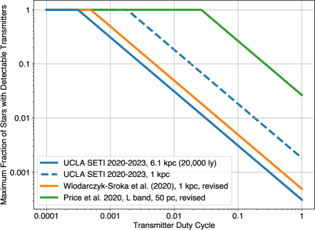
Figure 9: Upper limits on transmitter prevalence (95% CL) as a function of transmitter duty cycle. The solid blue line shows the limit calculated for GBT observations of 10,230 stars located within 20,000 ly of the Sun and analysis with the UCLA SETI pipeline, which has a conservative 94% probability of detecting detectable narrowband technosignatures (see text for detectability requirements). The dashed blue line shows the limit calculated for the subset of stars located within 1 kpc of the Sun. The solid and green orange lines show revisions to previously published limits (see Section 5.3 for correction factors).

5.3 Revisions to Published Estimates of Transmitter Prevalence

Many previous works ignored the dechirping efficiency and provided estimates of SETI search volumes or upper limits on the fraction of stars hosting transmitters under the assumption that the end-to-end efficiency of their pipeline was 100% or 50%. Our results show that the efficiency of a BL-like process is closer to 5.7% for drift rates within $\pm$8.88 Hz s^-1, 12.7% for drift rates within $\pm$4 Hz s^-1, and 25.3% for drift rates within $\pm$2 Hz s^-1, suggesting that the published estimates of search volumes and transmitter limits in previous works need revisions. We propose revised estimates below.

We suggest that the statement of Enriquez et al. (2017) that “fewer than $\sim$0.1% of the stellar systems within 50 pc possess these types of transmitters” ought to be rephrased as “fewer than $\sim$1.7% of the stellar systems within 50 pc possess the types of transmitters detectable in this search”. Focusing on their 692 primary targets only, which are stars within 50 pc, we can apply the formalism of Section 5.2 with $\eta_{p}=25.3\%$, which is appropriate for frequency drift rates up to $\pm$2 Hz s^-1 and BL data products with 51-fold incoherent averaging. We find that the upper limit on $f_{\rm TX}$ is 1.7% at the 95% confidence level for their 692 primary targets, which is a more realistic upper limit on the transmitter fraction.

Price et al. (2020) described the results of a search of 882, 1005, and 189 primary targets at L band, S band, and 10 cm, respectively, with drift rates up to $\pm$4 Hz s^-1 in data products with 51-fold incoherent averaging. They used a detection probability $p=50\%$ in their prevalence calculations, which yields 95% CL prevalence estimates of 0.68% at L band, 0.59% at S band, and 3.1% at 10 cm. These values are approximately 50% larger than those published by Price et al. (2020), which are 0.45%, 0.37%, and 2.0%, respectively, i.e., $\sim 2/n$. With the more realistic pipeline efficiency of $\eta_{p}=12.7\%$, we find an upper limit of $f_{\rm TX}=2.7\%$ at L band, suggesting that their upper limits must be revised upwards by a factor of $\sim$6.

Wlodarczyk-Sroka et al. (2020) improved the prevalence estimates by accounting for stars captured in the telescope beam in addition to the primary targets of Enriquez et al. (2017) and Price et al. (2020). However, they combined two data sets that are heterogeneous in their probabilities of detection success, which makes revision of their estimates difficult. Nevertheless, we can safely infer that their upper limit estimates must be revised upwards by approximately an order of magnitude, i.e., between the correction factors of 6 and 17 that we identified for these two surveys. For instance, their estimate of the incidence of star systems with detectable transmitters within 100 pc ought to be revised from 0.061% to $\sim$0.6%. Likewise, their estimate for main-sequence stars within 1 kpc of 0.005% ought to be revised to 0.05%, slightly larger than our 0.03% upper limit for stars within 20,000 ly. We found 1732 stars within 1 kpc in our observed sample (EIRP=$1.35\times 10^{15}$ W), which leads to an upper limit of transmitter prevalence of 0.18% for these stars with our observations. For this 1 kpc search volume, the prevalence estimate of Wlodarczyk-Sroka et al. (2020), with the correction presented here, is approximately three times more stringent than ours but required approximately 100 times more telescope time (506.5 hr vs. 5.2 hr of GBT L-band on-source integration time). Garrett & Siemion (2023)’s estimates for extragalactic transmitters require similar revisions.

Traas et al. (2021) observed 28 TESS targets with 28 cadences at L, S, C, and X band each, totaling $\sim$56 hr of on-source GBT time. They used a detection probability $p=50\%$ in their transmitter prevalence calculations. With their assumed pipeline efficiency, we find an upper limit to the fraction of observed stars with transmitters of 20.3% at the 95% confidence level, which is not identical to their estimate of 12.72%. Because they searched drift rates of up to $\pm$4 Hz s^-1 in data products with 51-fold incoherent averaging, a pipeline efficiency of $\eta_{p}=12.7\%$ is more appropriate, and their upper limits must be revised upwards by a factor of $\sim$6, leading to a weak limit of $\sim$80%.

Franz et al. (2022) searched 5, 17, 21, and 23 cadences of observations at L, S, C, and X band, capturing a total of 61 TESS TOIs in transit with $\sim$30 hr of GBT on-source time. If the pipeline efficiency were $\eta_{p}=50\%$, one might expect an upper limit on the fraction of stars with transmitters of 90.0%, 32.3%, 26.6%, and 24.4%, respectively, which differ from their values by more than $\sim$60%. However, the pipeline efficiency is closer to $\eta_{p}=12.7\%$, which leads to an inability to place an upper limit at the 95% confidence level at L, S, and C band, and a weak limit of $\sim$96% at X band.

5.4 Optical SETI

Shortly after Cocconi & Morrison (1959) proposed to search for interstellar communications in the radio part of the spectrum, Schwartz & Townes (1961) argued that similar searches could be conducted in the optical part of the spectrum. Townes (1983) suggested that searches in both the microwave and infrared parts of the spectrum were warranted. In this section, we recognize the value of searching at multiple wavelengths and briefly describe the results of a few optical SETI initiatives, being mindful that a review of this field is well beyond the scope of this work. Radio and optical SETI searches are most likely to be successful if presumptive civilizations operate beacons to emit distinctive signals, continuous or pulsed. Other information carriers such as charged particles, massive particles, gravitational waves, and neutrinos have been considered in the SETI context but are deemed inferior to photons for communication purposes (Hippke, 2018).

Howard et al. (2004) and Stone et al. (2005) described the results of multiyear targeted searches of several thousand stars for nanosecond pulses emitted by laser beacons. Tellis & Marcy (2017) adopted a different approach and searched for laser emission lines in high-resolution spectra of 5600 nearby stars. Maire et al. (2019) described the results of a search for near-infrared pulses from 1280 celestial objects.

The prevalence calculations from these optical SETI surveys outperform the radio SETI limits calculated for distances to 100 pc but not those calculated for larger distances. Tellis & Marcy (2017) ruled out “models of the Milky Way in which over 0.1% of warm, Earth-size planets harbor technological civilizations that, intentionally or not, are beaming optical lasers toward us.” Howard et al. (2004) published transmitter limits as a function of the transmitter repetition time. The fraction of stars with transmitting civilizations is also at most 0.1% in their work if one assumes repetition periods of $\sim 3\times 10^{4}$ h, which may be reasonable considering that it would take us approximately that long to beam a laser at all 331,312 stars within 100 pc with a 5 minute dwell time (equivalent duty cycle $D_{\rm opt}\simeq 3\times 10^{-6}$). The upper limit on transmitter prevalence that we obtained is $3\times 10^{-4}$, but only for transmitters with $D_{\rm radio}=100\%$.

From the point of view of the transmitting civilization, the requirements that an optical beacon be pointed at each one of tens of billions of stars is considerably more onerous than the equivalent requirement at radio wavelengths, where the entire sky can be covered much faster. For instance, the ratio of broadcast solid angles for beamwidths of 8.4 arcminute (GBT-class telescope at L band) and 1 arcsec (optical telescope, Townes, 1983) is $2.5\times 10^{5}$. This ratio also dictates the ratio of duty cycles $D_{\rm radio}/D_{\rm opt}$, which may justify the comparison with different values of the duty cycles in the paragraph above. To a civilization intent on broadcasting its existence, this intrinsic advantage of radio beacons may eclipse other considerations. However, we are unable to anticipate the choices of presumptive civilizations, and it behooves the SETI community to pursue a variety of search modalities.

6 Conclusions

Our observations of $\sim$11,680 stars and planetary systems with the GBT resulted in $\sim$37 million narrowband detections, none of which warranted reobservation.

A signal injection and recovery analysis of 10,000 chirp signals with randomly selected frequencies and drift rates revealed that the UCLA SETI pipeline recovers 94.0% of the injections and 98.7% of the injections outside of regions of dense RFI. Because the artificial signals were injected in raw voltage data, these percentages represent good estimates of the end-to-end pipeline efficiency for chirp signals.

A process that simulates the BL pipeline recovers a much smaller fraction of injections (5.7%), which we attribute largely to Doppler smearing of the signal that results from incoherent summing of 51 consecutive spectra. The characteristics of the recovered signals match the dechirping efficiency predictions of Margot et al. (2021) and confirm that the dechirping efficiency is an important factor that affects sensitivity, figure-of-merit, and transmitter prevalence calculations.

We developed a formalism for the calculation of upper limits on transmitter prevalence that take the end-to-end pipeline efficiency and transmitter duty cycle into account. We presented values calculated at the 95% confidence level for duty cycles of 100% and assumed that our observed sample is representative of the search volume. On the basis of our results and a Gaia survey of nearby (100 pc) stars, we can state that fewer than 6.6% of the 331,312 stars within 100 pc host a transmitter that is detectable in our survey (EIRP $>1.35\times 10^{13}$ W). If we extend the search volume to 1 kpc, the limit becomes 0.18% (EIRP $>1.35\times 10^{15}$ W). For stars located within 20,000 ly, we found that the fraction of stars with detectable transmitters (EIRP $>5.08\times 10^{16}$ W) is at most $3\times 10^{-4}$. Provided that the frequency and frequency drift rate fall within our search bounds, a sufficient condition for detection is the emission of a fixed-frequency or chirp waveform with bandwidth $<$ 3 Hz, 100% duty cycle, and minimum EIRP as stated above. We found that several previously published prevalence estimates need revisions with correction factors between 6 and 17.

We showed that the UCLA SETI pipeline can detect signals that had escaped the BL pipeline and were identified with AI techniques by Ma et al. (2023). In addition, we found that the AI detections are due to RFI, either because our pipeline correctly and automatically identified them as RFI, or because our usual visual inspection process showed them to be RFI.

We developed an improved Drake Figure of Merit for SETI search volume calculations that includes the pipeline efficiency and frequency drift rate coverage of a search. With this search volume metric, the UCLA SETI search to date falls in between the survey of 692 primary stars of Enriquez et al. (2017) and the survey of 1327 primary stars of Price et al. (2020).

UCLA SETI observations were designed, obtained, and analyzed by $\sim$130 undergraduate and $\sim$20 graduate students who have taken the annual SETI course since its first offering in 2016. 74 such students are coauthors of this work. The SETI course helps develop skills in astronomy, computer science, signal processing, statistical analysis, and telecommunications. Additional information about the course is available at https://seti.ucla.edu. UCLA SETI data are used in a citizen science collaboration called “Are we alone in the universe?”, which can be found at http://arewealone.earth.

Appendix A Sources

TOI	Disp.	$R_{p}$	Period	Insolation	$R_{s}$	Distance	RA	Dec
		($R_{\earth}$)	(days)	(Earth flux)	($R_{\sun}$)	(pc)	(hh:mm:ss)	(dd:mm:ss)
469.01	CP	3.55	13.63	60.16	1.01	68.19	06:12:13.88	-14:38:57.54
479.01	KP	12.68	2.78	615.47	1.02	194.55	06:04:21.53	-16:57:55.4
488.01	CP	1.12	1.20	58.26	0.35	27.36	08:02:22.47	03:20:13.79
536.01	KP	15.40	9.24	180.87	1.30	844.06	06:30:52.9	00:13:36.82
546.01	KP	13.44	9.20	203.95	1.12	726.41	06:48:46.71	-00:40:22.03
561.01	CP	2.74	10.78	73.35	0.84	85.80	09:52:44.44	06:12:57.97
562.01	CP	1.22	3.93	14.71	0.36	9.44	09:36:01.79	-21:39:54.23
571.01	KP	12.92	4.64	469.05	1.41	405.24	09:01:22.65	06:05:49.5
652.01	CP	2.11	3.98	464.96	1.03	45.68	09:56:29.64	-24:05:57.07
969.01	CP	3.65	1.82	167.63	0.82	77.26	07:40:32.8	02:05:54.92
1235.01	CP	1.89	3.44	134.67	0.63	39.63	10:08:52.38	69:16:35.83
1243.01	PC	4.49	4.66	8.59	0.49	43.19	09:02:55.83	71:38:11.1
1718.01	PC	4.40	5.59	219.06	0.94	52.30	07:28:04.33	30:19:18.24
1726.01	CP	2.24	7.11	145.57	0.90	22.40	07:49:55.05	27:21:47.28
1730.01	PC	2.76	6.23	114.27	0.53	35.69	07:11:27.8	48:19:40.56
1732.01	PC	2.55	4.12	38.33	0.63	74.76	07:27:12.35	53:02:42.97
1766.01	KP	16.72	2.70	1704.57	1.61	210.25	09:54:34.35	40:23:16.6
1774.01	CP	2.74	16.71	73.76	1.09	53.97	09:52:38.86	35:06:39.63
1775.01	PC	8.70	10.24	55.44	0.84	149.23	10:00:27.62	39:27:27.9
1776.01	PC	1.40	2.80	560.33	0.95	44.65	10:59:06.55	40:59:01.39
1779.01	KP	9.93	1.88	21.19	0.31	33.93	09:51:04.45	35:58:06.8
1789.01	CP	16.86	3.21	3000.05	2.26	229.07	09:30:58.42	26:32:23.98
1797.01	CP	2.99	3.65	283.72	1.05	82.34	10:51:06.41	25:38:27.83
1799.01	PC	1.63	7.09	163.47	0.96	62.13	11:08:55.9	34:18:10.85
1800.01	KP	12.42	4.12	459.54	1.26	277.28	11:25:05.98	41:01:40.87
1801.01	PC	1.99	10.64	10.73	0.55	30.68	11:42:18.14	23:01:37.32
1802.01	PC	2.51	16.80	5.92	0.58	60.69	10:57:01.28	24:52:56.42
1803.01	PC	4.22	12.89	18.34	0.69	119.24	11:52:11.07	35:10:18.48
1806.01	PC	2.84	15.15	2.15	0.40	55.52	11:04:28.36	30:27:30.87
1821.01	KP	2.43	9.49	41.92	0.77	21.56	11:14:33.04	25:42:38.15
1822.01	APC	14.57	9.61	192.62	1.71	312.52	11:11:06.68	39:31:36.02
1898.01	PC	9.17	45.52	8.34	1.61	79.67	09:38:13.27	23:32:48.29

Table 5: Characteristics of primary sources observed in 2020–2021. Columns show the TESS Object of Interest (TOI); the TESS Follow-up Observing Program Working Group disposition as of 2023 March 29 (Disp.), where PC is a planet candidate, CP is a confirmed planet, KP is a Kepler planet, and APC is an ambiguous planet candidate; the planet radius $R_{p}$ in Earth radii; the orbital period in days; the insolation in Earth flux units; the radius of the host star $R_{s}$ in solar radii; the distance in parsecs; and the right ascension and declination of the source.

TOI	Disp.	$R_{p}$	Period	Insolation	$R_{s}$	Distance	RA	Dec
		($R_{\earth}$)	(days)	(Earth flux)	($R_{\sun}$)	(pc)	(hh:mm:ss)	(dd:mm:ss)
1683.01	PC	2.64	3.06	163.06	0.70	51.19	04:23:55.12	27:49:20.53
1685.01	CP	1.32	0.67	204.71	0.46	37.62	04:34:22.55	43:02:13.34
1693.01	CP	1.42	1.77	57.02	0.46	30.79	06:01:14	34:46:23.13
1696.01	CP	3.17	2.50	13.81	0.28	64.92	04:21:07.36	48:49:11.39
1713.01	PC	4.65	0.56	3415.83	0.95	138.37	06:42:04.94	39:50:34.45
1730.01	PC	2.76	6.23	114.27	0.53	35.69	07:11:27.8	48:19:40.56
3772.01	PC	7.32	4.17	201.89	0.87	309.14	05:44:10.44	36:04:50.35
3795.01	PC	6.47	2.83	462.81	1.01	439.84	06:34:55.79	49:40:35.67
3800.01	PC	5.74	1.67	3970.53	1.40	598.89	06:53:06.26	39:07:56.2
4596.01	PC	2.72	4.12	186.21	0.98	93.49	06:34:49.88	27:23:16.86
4604.01	KP	1.56	2.23	476.88	0.92	90.06	05:05:47.03	21:32:53.52
4610.01	PC	1.56	3.11	114.27	0.69	47.91	05:16:10.38	30:35:06.26
5087.01	KP	3.38	17.31	10.89	0.77	59.25	04:29:39.09	22:52:57.24
5129.01	PC	3.64	7.41	57.53	1.19	201.91	06:38:48.67	29:05:21.56
1459.01	PC	2.49	9.16	66.15	0.82	101.36	01:17:26.83	26:44:45.42
1468.01	CP	2.01	15.53	2.14	0.37	24.74	01:06:36.93	19:13:29.71
1471.01	PC	3.92	20.77	37.34	0.97	67.55	02:03:37.2	21:16:52.78
4511.01	PC	3.09	20.90	42.72	1.00	121.83	03:17:13.27	15:30:06.22
4524.01	CP	1.69	0.93	876.25	1.11	63.68	03:16:42.75	15:39:22.88
4548.01	PC	5.37	4.60	84.87	1.59	165.59	02:25:21.87	25:31:50.44
4607.01	PC	3.08	5.51	262.94	1.31	180.02	01:55:37.25	24:07:05.35
4637.01	PC	2.81	14.35	38.49	0.86	112.15	02:13:03.56	19:24:09.6
4639.01	PC	2.88	3.99	502.42	1.03	205.74	01:49:15.49	21:42:12.57
4649.01	PC	2.75	15.08	68.57	1.01	148.25	01:59:49.57	16:20:48.1
5076.01	PC	3.13	23.44	13.56	0.85	82.86	03:22:02.5	17:14:21.15
5084.01	PC	1.16	5.83	37.73	0.75	21.36	03:03:49.09	20:06:38.12
5319.01	PC	3.75	4.08	38.79	0.48	61.17	02:20:51.25	23:31:13.59
5343.01	PC	2.50	12.84	39.96	0.69	120.86	03:12:06.25	24:32:00.82
5358.01	PC	2.92	2.66	148.44	0.80	138.71	03:36:44.14	28:33:00.97
5553.01	PC	1.55	1.76	439.12	0.81	103.35	02:52:00.52	15:03:20.39

Table 6: Characteristics of primary sources observed in 2022–2023. Columns as in Table 5.

References

- Anish Roshi et al. (2012) Anish Roshi, D., Bloss, M., Brandt, P., et al. 2012, Proceedings of the XXXth URSI General Assembly in Istanbul, August 2011, arXiv:1202.0938. https://arxiv.org/abs/1202.0938
- Bailer-Jones et al. (2021) Bailer-Jones, C. A. L., Rybizki, J., Fouesneau, M., Demleitner, M., & Andrae, R. 2021, AJ, 161, 147, doi: 10.3847/1538-3881/abd806
- Catling et al. (2018) Catling, D. C., et al. 2018, Astrobiology, 18, 709, doi: 10.1089/ast.2017.1737
- Cocconi & Morrison (1959) Cocconi, G., & Morrison, P. 1959, Nature, 184, 844, doi: 10.1038/184844a0
- Cohen et al. (1987) Cohen, R. J., et al. 1987, MNRAS, 225, 491, doi: 10.1093/mnras/225.3.491
- Drake (1984) Drake, F. 1984, SETI Science Working Group Report, ed. F. Drake, J. H. Wolfe, & C. L. Seeger, NASA Technical Paper No. TP-2244, 67–69
- Enriquez et al. (2017) Enriquez, J. E., Siemion, A., Foster, G., et al. 2017, ApJ, 849, 104, doi: 10.3847/1538-4357/aa8d1b
- Franz et al. (2022) Franz, N., Croft, S., Siemion, A. P. V., et al. 2022, AJ, 163, 104, doi: 10.3847/1538-3881/ac46c9
- Frigo & Johnson (2005) Frigo, M., & Johnson, S. G. 2005, IEEE Proceedings, 93, 216, doi: 10.1109/JPROC.2004.840301
- Friis (1946) Friis, H. 1946, Proceedings of the IRE, 34, 254, doi: 10.1109/JRPROC.1946.234568
- Fujii et al. (2018) Fujii, Y., et al. 2018, Astrobiology, 18, 739, doi: 10.1089/ast.2017.1733
- Gaia Collaboration (2023) Gaia Collaboration. 2023, A&A, 674, A1, doi: 10.1051/0004-6361/202243940
- Gaia Collaboration et al. (2021) Gaia Collaboration, Smart, R. L., Sarro, L. M., et al. 2021, A&A, 649, A6, doi: 10.1051/0004-6361/202039498
- Gajjar et al. (2021) Gajjar, V., Perez, K. I., Siemion, A. P. V., et al. 2021, AJ, 162, 33, doi: 10.3847/1538-3881/abfd36
- Garrett & Siemion (2023) Garrett, M. A., & Siemion, A. P. V. 2023, MNRAS, 519, 4581, doi: 10.1093/mnras/stac2607
- Harp et al. (2016) Harp, G. R., Richards, J., Tarter, J. C., et al. 2016, AJ, 152, 181, doi: 10.3847/0004-6256/152/6/181
- Hippke (2018) Hippke, M. 2018, Acta Astronautica, 151, 53, doi: 10.1016/j.actaastro.2018.05.038
- Horowitz & Sagan (1993) Horowitz, P., & Sagan, C. 1993, ApJ, 415, 218, doi: 10.1086/173157
- Howard et al. (2004) Howard, A. W., Horowitz, P., Wilkinson, D. T., et al. 2004, ApJ, 613, 1270, doi: 10.1086/423300
- Jovanovic & Levy (1997) Jovanovic, B. D., & Levy, P. S. 1997, The American Statistician, 51, 137, doi: 10.1080/00031305.1997.10473947
- Kogan (1998) Kogan, L. 1998, Radio Science, 33, 1289, doi: 10.1029/98RS02202
- Kraus (1986) Kraus, J. D. 1986, Radio Astronomy, 2nd edn. (Cygnus-Quasar Books)
- Lebofsky et al. (2019) Lebofsky, M., Croft, S., Siemion, A. P. V., et al. 2019, PASP, 131, 124505, doi: 10.1088/1538-3873/ab3e82
- Li & Margot (2023) Li, M., & Margot, J.-L. 2023, in American Astronomical Society Meeting Abstracts, Vol. 55, American Astronomical Society Meeting Abstracts, 440.05
- Ma et al. (2023) Ma, P. X., Ng, C., Rizk, L., et al. 2023, Nature Astronomy, 7, 492, doi: 10.1038/s41550-022-01872-z
- Maire et al. (2019) Maire, J., Wright, S. A., Barrett, C. T., et al. 2019, AJ, 158, 203, doi: 10.3847/1538-3881/ab44d3
- Margot et al. (2019) Margot, J. L., Croft, S., Lazio, J., Tarter, J., & Korpela, E. 2019, BAAS, 51, 298, doi: 10.48550/arXiv.1903.05544
- Margot et al. (2020a) Margot, J. L., Greenberg, A. H., Pinchuk, P., et al. 2020a, Data from: A search for technosignatures from 14 planetary systems in the Kepler field with the Green Bank Telescope at 1.15–1.73 GHz, v4, Dataset, doi: 10.5068/D1309D
- Margot et al. (2020b) Margot, J. L., Pinchuk, P., Geil, R., et al. 2020b, Data from: A search for technosignatures around 31 sun-like stars with the Green Bank Telescope at 1.15–1.73 GHz, Dataset, doi: 10.5068/D1937J
- Margot et al. (2021) Margot, J. L., Pinchuk, P., Geil, R., et al. 2021, AJ, 161, 55, doi: 10.3847/1538-3881/abcc77
- Margot et al. (2020c) Margot, J. L., Pinchuk, P., Greenberg, A. H., et al. 2020c, Data from: A search for technosignatures from TRAPPIST-1, LHS 1140, and 10 planetary systems in the Kepler field with the Green Bank Telescope at 1.15–1.73 GHz, v4, Dataset, doi: 10.5068/D1Z964
- Margot et al. (2018) Margot, J. L., Greenberg, A. H., Pinchuk, P., et al. 2018, AJ, 155, 209, doi: 10.3847/1538-3881/aabb03
- Meadows et al. (2022) Meadows, V., et al. 2022, arXiv e-prints, arXiv:2210.14293, doi: 10.48550/arXiv.2210.14293
- NASA Exoplanet Archive (2019) NASA Exoplanet Archive. 2019, Confirmed Planets Table, IPAC, doi: 10.26133/NEA1
- NASA Exoplanet Archive (2023) —. 2023, Planetary Systems, NExScI-Caltech/IPAC, doi: 10.26133/NEA12
- National Research Council (1982) National Research Council. 1982, Astronomy and astrophysics for the 1980’s. Volume 1: Report of the Astronomy Survey Committee., Vol. 1 (Washington, DC: The National Academies Press), doi: 10.17226/549
- National Research Council (1990) —. 1990, The Search for Life’s Origins: Progress and Future Directions in Planetary Biology and Chemical Evolution (Washington, DC: The National Academies Press), doi: 10.17226/1541
- Oliver & Billingham (1971) Oliver, B. M., & Billingham, J. 1971, Project Cyclops: A Design Study of a System for Detecting Extraterrestrial Intelligent Life, Tech. Rep. CR 114445, NASA
- Pinchuk & Margot (2022) Pinchuk, P., & Margot, J. L. 2022, AJ, 163, 76, doi: 10.3847/1538-3881/ac426f
- Pinchuk et al. (2019) Pinchuk, P., Margot, J.-L., Greenberg, A. H., et al. 2019, AJ, 157, 122, doi: 10.3847/1538-3881/ab0105
- Price et al. (2020) Price, D. C., Enriquez, J. E., Brzycki, B., et al. 2020, AJ, 159, 86, doi: 10.3847/1538-3881/ab65f1
- Qiao et al. (2020) Qiao, H.-H., et al. 2020, ApJS, 247, 5, doi: 10.3847/1538-4365/ab655d
- Rein et al. (2014) Rein, H., Fujii, Y., & Spiegel, D. S. 2014, Proceedings of the National Academy of Science, 111, 6871, doi: 10.1073/pnas.1401816111
- Schwartz & Townes (1961) Schwartz, R. N., & Townes, C. H. 1961, Nature, 190, 205, doi: 10.1038/190205a0
- Sheikh et al. (2019) Sheikh, S. Z., Wright, J. T., Siemion, A., & Enriquez, J. E. 2019, ApJ, 884, 14, doi: 10.3847/1538-4357/ab3fa8
- Siemion et al. (2013) Siemion, A. P. V., Demorest, P., Korpela, E., et al. 2013, ApJ, 767, 94, doi: 10.1088/0004-637X/767/1/94
- Stone et al. (2005) Stone, R. P. S., Wright, S. A., Drake, F., et al. 2005, Astrobiology, 5, 604, doi: 10.1089/ast.2005.5.604
- Tarter (2001) Tarter, J. 2001, Annual Review of Astronomy and Astrophysics, 39, 511, doi: 10.1146/annurev.astro.39.1.511
- Tarter et al. (2010) Tarter, J. C., Agrawal, A., Ackermann, R., et al. 2010, in Society of Photo-Optical Instrumentation Engineers (SPIE) Conference Series, Vol. 7819, Instruments, Methods, and Missions for Astrobiology XIII, 781902, doi: 10.1117/12.863128
- Taylor (1974) Taylor, J. H. 1974, A&AS, 15, 367
- Technosignatures Workshop Participants (2018) Technosignatures Workshop Participants, N. 2018, arXiv e-prints, doi: 10.48550/arXiv.1812.08681
- Tellis & Marcy (2017) Tellis, N. K., & Marcy, G. W. 2017, AJ, 153, 251, doi: 10.3847/1538-3881/aa6d12
- Townes (1983) Townes, C. H. 1983, Proceedings of the National Academy of Science, 80, 1147, doi: 10.1073/pnas.80.4.1147
- Traas et al. (2021) Traas, R., Croft, S., Gajjar, V., et al. 2021, AJ, 161, 286, doi: 10.3847/1538-3881/abf649