Scalable Computation of Causal Bounds

Abstract

We consider the problem of computing bounds for causal queries on causal graphs with unobserved confounders and discrete valued observed variables, where identifiability does not hold. Existing non-parametric approaches for computing such bounds use linear programming (LP) formulations that quickly become intractable for existing solvers because the size of the LP grows exponentially in the number of edges in the causal graph. We show that this LP can be significantly pruned, allowing us to compute bounds for significantly larger causal inference problems compared to existing techniques. This pruning procedure allows us to compute bounds in closed form for a special class of problems, including a well-studied family of problems where multiple confounded treatments influence an outcome. We extend our pruning methodology to fractional LPs which compute bounds for causal queries which incorporate additional observations about the unit. We show that our methods provide significant runtime improvement compared to benchmarks in experiments and extend our results to the finite data setting. For causal inference without additional observations, we propose an efficient greedy heuristic that produces high quality bounds, and scales to problems that are several orders of magnitude larger than those for which the pruned LP can be solved.

Keywords: Causal Bounds, Partial Identification of Causal Effects, Causal Bounds with Observations, Multi-Cause Setting with Unobserved Confounders, Linear Programming

1 Introduction

We are interested in answering the following counterfactual query about a large-scale system of discrete variables: What will be the value of some outcome variables $V_{O}$ if we intervene on variables $V_{I}$, given the values of variables $V_{A}$ are known? Several meaningful questions in data-rich environments can be formulated this way. As an example, consider the causal graph in Figure 1 that describes the health outcome of a patient $Y$ as a function of a sequence of treatments administered $T_{i}$ by a physician, $i=1,\ldots,5$. The treatments chosen are functions of some patient characteristics $C_{i}$, $i=1,2$, e.g. sex and age. The variable $U_{B}$ refers to unknown variables, also known as confounders, that might impact both the choice of treatments and the health outcome e.g. patient lifestyle, physician biases, etc. What will be the expected health outcome $Y$ of the patient if she is administered treatments $T_{i},i=1,\ldots,5$, given her sex and age are known? (Ranganath and Perotte, 2019; Janzing and Schölkopf, 2018; D’Amour, 2019; Tran and Blei, 2017)

Traditional approaches to estimate causal effects of interventions involve randomized control trials (RCTs) in order to remove the impact of confounders. However, running experiments to identify personalized interventions for sub-populations of units is often expensive and practically infeasible. Therefore, there is a push to develop techniques that can use observational data that is far more readily available.

The challenge in observational studies is to account for unobserved confounders which can create spurious correlations and adversely impact data-driven decision-making (Imbens and Rubin, 2015; Pearl, 2009). For example, the unknown confounder $U_{B}$ in Figure 1 influences both the prescribed treatments and the outcome: a patient who exercises regularly may have lower body weight, and thus, require lower dosage of treatments, but also have an improved response to treatments. Hence, treatment dosage can be negatively correlated with treatment response, although administering lower dosage of treatments need not result in improved response. Hence, alternate methodologies need to be developed to compute the causal effect of treatments on health outcomes in the presence of unobserved confounders.

Figure 1: $C_{1}$ and $C_{2}$ denote the sex and age of the patient. These influence the treatments, $T_{i},i=1\ldots 5$, which the patient is prescribed. Note that the prescription of one treatment can influence the prescription of another (e.g. $T_{3}$ is prescribed to manage the side effects of $T_{1}$). Together, these variables influence $Y$, the health outcome of the patient. Unobserved confounder $U_{B}$ denotes unobserved variables, e.g. patient lifestyle, physician biases, that impact the choice of treatments, and the health outcome.

While it is impossible to precisely identify causal effects in the presence of unobserved confounders, it is possible to obtain bounds on the causal query, the causal effect of interest. There have been multiple such attempts to bound causal effects for small special graphs. Evans (2012) bound causal effects in the special case where any two observed variables are neither adjacent in the graph, nor share a latent parent. Richardson et al. (2014) bound the causal effect of a treatment on a parameter of interest by invoking additional (untestable) assumptions and assess how inference about the treatment effect changes as these assumptions are varied. Kilbertus et al. (2020) and Zhang and Bareinboim (2021) develop algorithms to compute causal bounds for extensions of the instrumental variable model in a continuous setting. Geiger and Meek (2013) bound causal effects in a model under specific parametric assumptions. Finkelstein and Shpitser (2020) develop a method for obtaining bounds on causal parameters using rules of probability and restrictions on counterfactuals implied by causal graphs.

While fewer in number, there have also been attempts to bound causal effects in large general graphs. Poderini et al. (2020) propose techniques to compute bounds in special large graphs with multiple instruments and observed variables. Finkelstein et al. (2021) propose a method for partial identification in a class of measurement error models, and Zhang et al. (2022) and Duarte et al. (2021) propose a polynomial programming based approach to solve general causal inference problems, but their procedure is computationally intensive for large graphs.

In this work, we extend the class of large graphs for which causal effects can be efficiently bounded. In particular, we focus on a class of causal inference problems where causal bounds can be obtained using linear programming (LP) (Balke and Pearl, 1994; Zhang and Bareinboim, 2017; Pearl, 2009; Sjölander et al., 2014). Recently, Sachs et al. (2022) identified a large problem class for which LPs can be used to compute causal bounds, and have developed an algorithm for formulating the objective function and the constraints of the corresponding LP. This problem class is a generalization of the instrumental variable setting, and is thus widely applicable. However, as we describe later, the size of the LP is exponential in the number of edges in the causal graph, and therefore, the straightforward formulation of the LP can be tractably solved only for very small causal graphs. In this work, we show how to use the structure of the causal query and the underlying graph to significantly prune the LP, and as a consequence, significantly increase the size of the graphs for which the LP method remains tractable. This work is the full version of (Shridharan and Iyengar, 2022) and extends the pruning methodology to fractional linear programs that are used to compute bounds for causal inference problems with additional observations about the unit. Our main contributions are as follows:

1. In Section 3 we show that the exponential number of variables in the LP used to compute causal bounds can be aggregated to reduce the number of variables by several orders of magnitude without impacting the quality of the bound – compare $|R|$ with $|H|$ in Table 1.

2. Although we show the bounds can be computed by solving a much smaller LP, we get this computational advantage only if the pruned LP can be constructed efficiently. In Section 3 we show that the pruned LP can be constructed directly, i.e. without first constructing the original LP or iterating over its variables. These results critically leverage the structure of the LP corresponding to a causal inference problem. In particular, they leverage the fact that all possible functions from the parents $pa(V)$ to a variable $V$ are admissible.

3. In Section 4 we show that the structural results that help us construct the pruned LP lead to closed form bounds for a class of causal inference problems. This class of problems includes as a special case the well-studied setting in Figure 1 where multiple confounded treatments influence a outcome. Moreover, we are able to compute these bounds even when there are causal relationships between the treatments.

4. In Section 5 we extend our pruning methodology to compute bounds for causal queries with additional observations about the unit. In this setting, the bounds are computed using fractional LPs. We show that the fractional LP can be converted into an LP, and then show how this LP can be pruned.

5. In Section 6.3, we propose a simple greedy heuristic to compute approximate solutions for the pruned LPs when there are no additional observations. We show that this heuristic allows us to compute approximate bounds for much larger graphs with very minimal degradation in performance.

The organization of the rest of this paper is as follows. In Section 2 we introduce our formalism. In Section 3 we introduce our main structural results for pruning the LPs. In Section 4 we show that the LP bounds can be computed in closed form for a large class of problems and also discuss an example of this class of problems. In Section 5 we show how to incorporate additional observations about the unit in the query to compute updated bounds. In Section 6 we report the results of numerical experiments validating and extending the methods proposed in Sections 3 and 5. In particular, we show the significant runtime improvement provided by our methods compared to benchmarks and extend all results in earlier sections to the finite data setting. In Section 6.3 we introduce our greedy heuristic and benchmark its performance. Section 7 discusses possible extensions.

2 Causal Inference Problems

Let $G$ denote the causal graph. Let $V_{1},\ldots,V_{n}$ denote the variables in $G$ in topologically sorted order, and $N=\{1,\ldots,n\}$ denote the set of indices for the variables. We assume that each variable $V_{i}\in\{0,1\}$. Later in this section we discuss why our proposed techniques automatically apply to the case where $V_{i}$ takes discrete values. We use lower case letters for the values for the variables, and the notation $V_{i}=v_{i}$ denotes that the variable $V_{i}$ takes the value $v_{i}\in\{0,1\}$. For any subset $S\subseteq N$, we define $V_{S}:=\{V_{i}:i\in S\}$, and the notation $V_{S}=v_{S}$ denotes the variable $V_{i}=v_{i}$, for all $i\in S$, for some $v\in\{0,1\}^{|N|}$.

We consider a class of “partitioned” causal graphs with two sets of variables, $V_{A}$ and $V_{B}$, where $V_{B}$ topologically follow $V_{A}$ (Sachs et al. (2020)). The $V_{A}$ variables represent contextual or demographic variables (e.g. gender and age of a patient, past purchases, etc.) for a unit, and are always observed. For example, in Figure 1, $V_{A}=\{C_{i}:i=1,2\}$, the patient characteristics. The $V_{B}$ variables can be observed, intervened upon or are the outcomes of interest in a query. In Figure 1 $V_{B}=\{Y\}\cup\{T_{i}:i=1,\ldots,5\}$.

Assumption 1 (Sachs et al. (2022))

The index set $N$ is partitioned into two sets $N=A\cup B$, where

1. $V_{B}$ topologically follow $V_{A}$,

2. each variable in $V_{A}$ has no parents, but is the parent of some variable in $V_{B}$.

3. $V_{B}$ variables can have a common unobserved confounder $U_{B}$, and

4. no pair of variables $(V_{i},V_{j})$, where $i\in A$ and $j\in B$, can share an unobserved confounder.

For example, in the causal graph in Figure 2, $V_{A}=\{Z\}$ and $V_{B}=\{X,Y\}$.

Figure 2: Causal Graph for Running Example with query $\mathcal{Q}=\mathbb{P}(Y(X=1)=1|Z=1)$

We assume that the conditional probability distribution $p_{v_{B}.v_{A}}=\mathbb{P}(V_{B}=v_{B}|V_{A}=v_{A})$ is known. In Section 6.2 we extend our results to the finite data setting where the estimate $\bar{p}_{v_{B}.v_{A}}\neq p_{v_{B}.v_{A}}$. Our goal is to compute bounds for counterfactual queries of the form $\mathcal{Q}=\mathbb{P}\big{(}V_{O}(V_{I}=q_{I})=q_{O}|V_{A}=q_{A}\big{)}$, i.e. the probability of the outcome $V_{O}=q_{O}$ after an intervention $do(V_{I}=q_{I})$ given contextual information for $V_{A}$. This counterfactual is specific to an individual realization of $V_{A}$, and computes the outcome of $V_{O}$ if $V_{I}$ was set to $q_{I}$. In order to simplify our results we impose a restriction on $I$ that does not impact the query.

Definition 2 (Critical variables for a query $\mathcal{Q}$)

Let $G^{do(V_{I}=q_{I})}$ denote the mutilated graph after intervention $do(V_{I}=q_{I})$, i.e. variables $V_{I}$ no longer have any incoming arcs. Then the critical variables $V_{C(\mathcal{Q})}$ for the query $\mathcal{Q}$ denote the set of variables in $V_{A}\cup V_{B}$ that have a path to some variable in $V_{O}$ in $G^{do(V_{I}=q_{I})}$.

Assumption 3 (Valid Query)

The query $\mathcal{Q}=\mathbb{P}\big{(}V_{O}(V_{I}=q_{I})=q_{O}|V_{A}=q_{A}\big{)}$ satisfies the following conditions:

1. $O$, $I\subseteq B$, with $O\cap I=\emptyset$.

2. All variables $V_{I}\subseteq V_{C(\mathcal{Q})}$, i.e. all $V_{I}$ variables are critical for the query.

Lemma 15 in Appendix A establishes that ii is without loss of generality since any $V_{i}\in V_{I}$ that is not critical can be removed from the query. Note that the class of problems defined in Sachs et al. (2022) allow the variables in $V_{A}$ to have parents, but also require every variable in $V_{A}$ that has a directed path to some variable in $V_{B}$ in $G^{do(V_{I}=q_{I})}$ to be intervened upon, and so these variables therefore cannot have parents in $G^{do(V_{I}=q_{I})}$. Thus, the assumption in Sachs et al. (2022) is effectively equivalent to our assumption that variables in $V_{A}$ do not have parents. Furthermore, we assume that every variable in $V_{A}$ is the parent of some variable in $V_{B}$, and provides context in the query. Our assumption is more interpretable and broadly applicable, yet maintains the expressibility of the Sachs et al. (2022) formulation.

For graphs satisfying Assumption 1, the unobserved confounder $U_{B}$ can potentially be very high dimensional with an unknown structure. We circumvent the difficulty of modeling $U_{B}$ directly, by instead modeling the impact of the confounder on the relationships between the observed variables. For $j\in B$, let $pa(V_{j})$ denote the parents of $V_{j}$ in the causal graph. Then the variable $V_{j}=f_{j}(pa(V_{j}),U_{B})$ for some unknown but fixed function $f_{j}:\{0,1\}^{|pa(V_{j})|}\times\mathcal{U}_{B}\mapsto\{0,1\}$, where $\mathcal{U}_{B}$ denotes the domain of $U_{B}$. Therefore, the confounder $U_{B}$ impacts the relationship between $pa(V_{j})$ and $V_{j}$ by selecting a function $f_{j}\in\mathcal{F}_{j}=\{f:f\text{ is a function from }pa(V_{j})\mapsto V_{j}\}$. In the causal graph in Figure 2, for each fixed value for the unknown confounder $U$, the variable $X$ is a function of $Z$; thus, $U$ effectively selects one function from the set $\mathcal{F}=\{f\text{ is a function from }Z\mapsto X\}$. Similarly, $U$ selects one function from the set $\mathcal{G}=\{g:g\text{ is a function from }X\mapsto Y\}$.

Since each variable $V_{k}\in pa(V_{j})$ takes values in $\{0,1\}$ and $V_{j}\in\{0,1\}$, the cardinality of the set $|\mathcal{F}_{j}|=2^{2^{|pa(V_{j})|}}$. Therefore, the elements of $\mathcal{F}_{j}$ can be indexed by the set $R_{V_{j}}=\{1,\ldots,|\mathcal{F}_{j}|\}$. Let $f_{j}(\cdot,r_{V_{j}}):pa(V_{j})\mapsto V_{j}$ denote the $r_{V_{j}}$-th function in $\mathcal{F}_{j}$. Let the set $R=\prod_{j\in B}R_{V_{j}}$ index all possible mappings from $pa(V_{j})\mapsto V_{j}$ for all $j\in B$. Thus, the response function variable $r=(r_{V_{|A|+1}},\ldots r_{V_{n}})\in R$ completely models the impact of $U_{B}$, i.e. the values of variables $V_{B}$ is a deterministic function of $V_{A}$ and $r$. For example, in the causal graph in Figure 2, it is easy to see that $|\mathcal{F}|=|\mathcal{G}|=4$, and the set $R=\{(r_{X},r_{Y})=\{1,\ldots,4\}^{2}\}$, where $f_{r_{X}}$ denotes the $r_{X}$-th function from $\mathcal{F}$ and $g_{r_{Y}}$ denotes the $r_{Y}$-th function from $\mathcal{G}$. Note that the cardinality $|R|=\prod_{j\in B}2^{2^{|pa(V_{j})|}}$ is exponential in the number of arcs in the causal graph.

Note that although we work with causal graphs with binary variables in this paper, generalizing all subsequent results to categorical variables is straightforward. The critical property that we exploit is that the set of response function variables index possible mappings between variables. Therefore, our approach can be extended to general categorical variables by suitably defining response function variables. For example, suppose in Figure 2, $X,Y\in\{0,\ldots,m\}$. Then the response function variable $r_{Y}\in\{0,\ldots,m^{m}-1\}$. All our results generalize to this more general setting.

The unknown distribution over the high dimensional $U_{B}$ can be equivalently modeled via the distribution $\bm{q}\in\mathbb{R}^{|R|}_{+}$ over the set $R$. For $r\in R$, let $F_{T}(V_{S}=v_{S},r)$ denote the value of $V_{T}\subseteq V_{B}$ when $V_{S}=v_{S}$ provided it is well defined. As discussed, setting $V_{A}=v_{A}$ and choosing $r\in R$ completely defines the values for $V_{B}$, i.e. $F_{B}(V_{A}=v_{A},r)$ is well defined. Let

$$R_{v_{B}.v_{A}}=\{r:F_{B}(V_{A}=v_{A},r)=v_{B}\}.$$ (1)

Hence, $p_{v_{B}.v_{A}}=\sum_{r\in R_{v_{B}.v_{A}}}q_{r}$. For example, in the causal graph in Figure 2, $R_{xy.z}=\{(r_{X},r_{Y}):f_{r_{X}}(z)=x,g_{r_{Y}}(x)=y\}$ denotes the set of $r$-values that map $z\mapsto(x,y)$. Hence, $\mathbb{P}(X=x,Y=y|Z=z)=\sum_{(r_{X},r_{Y})\in R_{xy.z}}q_{r_{X}r_{Y}}$.

The set

$$R_{\mathcal{Q}}=\big{\{}r\in R:F_{O}\big{(}(V_{A},V_{I})=(q_{A},q_{I}),r\big{)}=q_{O}\big{\}}$$ (2)

denotes the set of $r$ values consistent with the query $\mathcal{Q}=\mathbb{P}(V_{O}(V_{I}=q_{I})=q_{O}|V_{A}=q_{A})$. Hence, $\mathbb{P}(V_{O}(V_{I}=q_{I})=q_{O}|V_{A}=q_{A})=\sum_{r\in R_{\mathcal{Q}}}q_{r}$. For the query $\mathcal{Q}=\mathbb{P}(Y(X=1)=1|Z=1)$ in the causal graph in Figure 2, the set $R_{\mathcal{Q}}=\left\{(r_{X},r_{Y}):g_{r_{Y}}(1)=1\right\}$.

Then lower and upper bounds for the causal query can be obtained by solving the following pair of linear programs (Balke and Pearl (1994); Sachs et al. (2022)):

$$\begin{array}[]{rl}\alpha_{L}/\alpha_{U}=\min_{q}/\max_{q}&\sum_{r\in R_{\mathcal{Q}}}q_{r}\\ \text{s.t.}&\sum_{r\in R_{v_{B}.v_{A}}}q_{r}=p_{v_{B}.v_{A}},\ \forall v_{A},v_{B},\\ &q\geq 0.\end{array}$$ (3)

Recall for $V_{A}=v_{A}$, $r\in R$ uniquely determines the value of $V_{B}$. Hence, for fixed $v_{A}$, $\cup_{v_{B}}R_{v_{B}.v_{A}}$ is a partition of $R$. Thus, the constraint $\sum_{r\in R}q_{r}=\sum_{v_{B}}\sum_{r\in R_{v_{B}.v_{A}}}q_{r}=\sum_{v_{B}}p_{v_{B}.v_{A}}=1$ is implied by the other constraints in the LP, and therefore, is not explicitly added to the LP.

Note that our bounds are valid even if faithfulness assumptions are violated (Andersen, 2013). However, our results only leverage conditional independence relationships encoded in the graph, and not additional conditional independence relationships in the data. Hence, if the data displays additional independence relationships, our method is unable to leverage it to compute tighter bounds. Note also that we do not impose any additional constraints on the unobserved confounder.

3 Pruning the LP

In this section, we show how to reduce the size of the LPs (3) by aggregating variables. Let $h:V_{A}\rightarrow V_{B}$ denote any function $V_{A}\mapsto V_{B}$. We also refer to $h$ as a hyperarc since it can be interpreted as an arc in a hypergraph. We show how to reformulate LP (3) into another equivalent LP with variables indexed by hyperarcs, instead of response function variables. The number of possible hyperarcs is $(2^{|B|})^{2^{|A|}}\ll|R|$ (see Table 1). Hence, the new LP has at most $(2^{|B|})^{2^{|A|}}$ variables, and is thus exponentially smaller than LP (3). Furthermore, we show we only need to consider a smaller set of hyperarcs that are “valid” given the structure of the causal graph.

Recall that $F_{B}(V_{A}=v_{A},r)$ denotes the value of $V_{B}$ when $V_{A}=v_{A}$ and $r\in R$. Let

$$R_{h}=\left\{r\in R:F_{B}(V_{A}=v_{A},r)=h(v_{A}),\ \forall v_{A}\in\{0,1\}^{|A|}\right\}$$ (4)

denote the set of $r$ values consistent with the hyperarc $h$, i.e. the set of $r$’s that map $V_{A}=v_{A}$ to $V_{B}=h(v_{A})$ for all inputs $v_{A}\in\{0,1\}^{|A|}$. For the graph in Figure 2,

$$R_{h}=\left\{(r_{X},r_{Y})\in R:\begin{array}[]{l}\big{(}f_{r_{X}}(0),g_{r_{Y}}(f_{r_{X}}(0))\big{)}=h(0)\\ \big{(}f_{r_{X}}(1),g_{r_{Y}}(f_{r_{X}}(1))\big{)}=h(1)\end{array}\right\}$$

The causal graph structure implies that $R_{h}\neq\emptyset$ only for a subset of hyperarcs.

Definition 4 (Valid Hyperarc)

A hyperarc $h$ is valid if $R_{h}\neq\emptyset$.

In Section 3.1, we discuss why $R_{h}\neq\emptyset$ only for a subset of hyperarcs, and how to efficiently check the validity of a hyperarc. We denote the set of valid hyperarcs by $H$.

Next, we show how to write the LP in terms of variables $q_{h}=\sum_{r\in R_{h}}q_{r}$ corresponding to hyperarcs $h\in H$ by aggregating variables $q_{r}$ for $r\in R_{h}$. In Lemma 14 in Appendix A we establish that $R=\cup_{h\in H}R_{h}$ is a partition of $R$. Therefore,

$$\sum_{r\in R_{v_{B}.v_{A}}}q_{r}=\sum_{h\in H}\sum_{r\in R_{h}\cap R_{v_{B}.v_{A}}}q_{r}=\sum_{\{h\in H:h(v_{A})=v_{B}\}}\Big{[}\sum_{r\in R_{h}}q_{r}\Big{]}=\sum_{\{h\in H:h(v_{A})=v_{B}\}}q_{h}.$$

Thus, the constraints in (3) can all be formulated in terms of the variables $q_{h}$ corresponding to hyperarcs.

Next, consider the objective for the minimization LP:

$$\min\ \sum_{r\in R}\boldsymbol{1}\{r\in R_{\mathcal{Q}}\}q_{r}=\min\ \sum_{h\in H}\sum_{r\in R_{h}}\boldsymbol{1}\{r\in R_{\mathcal{Q}}\}q_{r}$$

From the definition of $R_{h}$, it follows that all $q_{r}$, $r\in R_{h}$, have a coefficient $1$ in the same set of constraints, namely those indexed by $\{(v_{B}=h(v_{A}),v_{A}):v_{A}\in\{0,1\}^{|A|}\big{\}}$. Hence, for any fixed value $q_{h}$ for the variable corresponding to hyperarc $h$, any allocation in the set $\{[q_{r}]_{r\in R_{h}}:q_{h}=\sum_{r\in R_{h}}q_{r},q_{r}\geq 0,r\in R_{h}\}$ is feasible. Hence, any optimal allocation satisfies

$$\min\Big{\{}\sum_{r\in R_{h}}\boldsymbol{1}\{r\in R_{\mathcal{Q}}\}q_{r}:\sum_{r\in R_{h}}q_{r}=q_{h},q_{r}\geq 0,\forall r\in R_{h}\Big{\}}=\Big{(}\min_{r\in R_{h}}\boldsymbol{1}\{r\in R_{\mathcal{Q}}\}\Big{)}q_{h}$$

Hence the lower bound LP can be reformulated as

$$\begin{array}[]{rll}\min_{q}&\sum_{h\in H}c^{L}_{h}q_{h}\\ \text{s.t.}&\sum_{h\in H:h(v_{A})=v_{B}}q_{h}=p_{v_{B}.v_{A}},&\forall v_{A},v_{B},\\ &q\geq 0,\end{array}$$ (5)

where

$$c^{L}_{h}:=\min_{r\in R_{h}}\boldsymbol{1}\{r\in R_{\mathcal{Q}}\}=\boldsymbol{1}\{R_{h}\subseteq R_{\mathcal{Q}}\}.$$ (6)

The objective for the upper bound is given by

$$\max\ \sum_{r\in R}\boldsymbol{1}\{r\in R_{\mathcal{Q}}\}q_{r}=\max\ \sum_{h\in H}\sum_{r\in R_{h}}\boldsymbol{1}\{r\in R_{\mathcal{Q}}\}q_{r}=\max\ \sum_{h\in H}\Big{(}\max_{r\in R_{h}}\boldsymbol{1}\{r\in R_{\mathcal{Q}}\}\Big{)}q_{h},$$

where the second equality follows from an argument similar to the one used to establish the objective for the lower bound LP. Thus, the upper bound LP is given by

$$\begin{array}[]{rll}\max_{q}&\sum_{h\in H}c_{h}^{U}q_{h}\\ \mbox{s.t.}&\sum_{h\in H:h(v_{A})=v_{B}}q_{h}=p_{v_{B}.v_{A}},&\forall v_{A},v_{B}\\ &q\geq 0,\end{array}$$ (7)

where

$$c^{U}_{h}=\max_{r\in R_{h}}\boldsymbol{1}\{r\in R_{\mathcal{Q}}\}=\boldsymbol{1}\{R_{h}\cap R_{\mathcal{Q}}\neq~{}\emptyset\}.$$ (8)

Both reformulations have exponentially fewer variables since $|H|\ll|R|$; however, they are useful only if the set of valid hyperarcs $H$ and the corresponding coefficients $\boldsymbol{1}\{R_{h}\subseteq R_{\mathcal{Q}}\}$ and $\boldsymbol{1}\{R_{h}\cap R_{\mathcal{Q}}\neq\emptyset\}$ can be efficiently computed, i.e. in particular, without formulating the original LPs or iterating over $R$. In Section 3.1 we describe how to efficiently check the validity of a hyperarc and efficiently compute $H$, and in Section 3.2 (resp. Section 3.3) we show how to efficiently compute $c^{L}_{h}$ (resp. $c^{U}_{h}$). Finally, in Section 3.4, we describe our procedure that uses results established in Sections 3.1, 3.2 and 3.3 to efficiently construct pruned LPs (5) and (7) without formulating the original LPs or iterating over $R$.

3.1 Characterizing Valid Hyperarcs

We now discuss why $R_{h}\neq\emptyset$ only for a subset of hyperarcs. We also show how to efficiently check the validity of hyperarc $h$ without enumerating all values in the set $R$ to check if there exists $r\in R$ such that $F_{B}(V_{A}=v_{A},r)=h(v_{A})$ for all $v_{A}\in\{0,1\}^{|A|}$ i.e. $R_{h}\neq\emptyset$. Instead, we show that the outputs of the function $h$ alone are sufficient to determine its validity. We motivate the main result of this section by first considering the simple causal graph in Figure 2. Consider a hyperarc $h$ with $h(0)=(x_{0},y_{0})$ and $h(1)=(x_{1},y_{1})$ for $x_{i},y_{i}\in\{0,1\}$, $i=0,1$. Note that for any choice of $x_{i}$ and $y_{i}$, $i=0,1$, $h$ is a hyperarc from $Z\mapsto(X,Y)$. For $h$ to be a valid hyperarc, it should be of the form $h(z)=(f_{h}(z),g_{h}(f_{h}(z)))$ for some $f_{h}\in\mathcal{F}$ and $g_{h}\in\mathcal{G}$. The functions (if they exist) must satisfy:

$$f_{h}(z)=\begin{cases}x_{0}&\text{if }z=0\\ x_{1}&\text{if }z=1\end{cases}\qquad g_{h}(x)=\begin{cases}y_{0}&\text{if }x=x_{0}\\ y_{1}&\text{if }x=x_{1}\end{cases}$$

Clearly, $f_{h}$ is well defined for any choice of $x_{i}$, $i=0,1$. However, there exists $g_{h}$ satisfying the conditions above if, and only if, $y_{0}=y_{1}$ whenever $x_{0}=x_{1}$. Hence, $h\not\in H$ if, and only if, $x_{0}=x_{1}$ but $y_{0}\neq y_{1}$. For example, consider the hyperarc $h_{1}$ with $h_{1}(0)=(0,0)$ and $h_{1}(1)=(0,0)$. To check if $h_{1}$ is valid, we need to check if there exists well defined functions $f_{h_{1}}:Z\mapsto X$ and $g_{h_{1}}:X\mapsto Y$ which satisfy:

$$f_{h_{1}}(z)=\begin{cases}0&\text{if }z=0\\ 0&\text{if }z=1\end{cases}\qquad g_{h_{1}}(x)=0,\quad\text{if }x=0\\$$

Clearly, $f_{h_{1}}$ is a well defined function. Any function $g:X\mapsto Y$ in $\mathcal{G}$ with $g(0)=0$ satisfies the conditions for $g_{h_{1}}$. Hence, $h_{1}\in H$.

On the other hand, consider the hyperarc $h_{2}$ with $h_{2}(0)=(0,0)$ and $h_{2}(1)=(0,1)$. The hyperarc $h_{2}$ is valid if there exists a well defined function $g_{h_{2}}:X\mapsto Y$ which satisfies:

$$g_{h_{2}}(x)=\begin{cases}0&\text{if }x=0\\ 1&\text{if }x=0\\ \end{cases}$$

Clearly, there cannot be such a function, and so $h_{2}\not\in H$.

Note that we did not have to iterate over the set $R$ to check if a hyperarc $h$ is valid. Instead, we recognize that a hyperarc $h$ only partially specifies a function mapping from $pa(V_{j})$ to $V_{j}$. Therefore, in order to check the validity of $h$, we only need to check if there exists some binary function $pa(V_{j})\rightarrow V_{j}$ which satisfies this partial specification. Hence, the outputs of the function $h$ alone are sufficient to determine its validity. The following theorem generalizes this observation to general causal graphs.

Theorem 5 (Valid hyperarcs)

Let $a_{A}\in\{0,1\}^{|A|}$ denote the values set for the variables $V_{A}$, and let $a_{B}=h(a_{A})\in\{0,1\}^{|B|}$ denote the values for the variables $V_{B}$ when the hyperarc $h$ is evaluated at $a_{A}$. A hyperarc $h$ is valid if, and only if, for all $\big{(}a_{A},a_{B}=h(a_{A})\big{)},\big{(}b_{A},b_{B}=h(b_{A})\big{)}\in\{0,1\}^{|N|}$ and $j\in B$,

$$a_{P_{j}}=b_{P_{j}}\implies a_{j}=b_{j},$$ (9)

where $P_{j}\subseteq N$ denote the indices of $pa(V_{j})$.

Proof  It is clear that if a hyperarc is valid, then it is satisfies (9).

Suppose a hyperarc satisfies (9). Then we are given a partial specification for a function from $pa(V_{j})\rightarrow V_{j}$, i.e. the same input values are always mapped to the same output value; however, the output is only specified for possibly a subset of input values. For each $V_{j}\in V_{B}$, $r_{V_{j}}$ indexes the set of all possible functions $pa(V_{j})\rightarrow V_{j}$; therefore, for every node $j$ there exists a binary function $pa(V_{j})\rightarrow V_{j}$ which satisfies the partial specification given by the hyperarc $h$. Thus, $R_{h}\neq\emptyset$, or equivalently, $h$ is valid.  
Theorem 5 implies that we only have to search through the set of possible hyperarcs from $V_{A}\mapsto V_{B}$ of cardinality $2^{|B|2^{|A|}}$ for hyperarcs which satisfy (9) to identify the set $H$ of valid hyperarcs. The first two columns of Table 1 compare $|R|$ with the maximum possible number of hyperarcs $2^{|B|2^{|A|}}$ for seven different causal inference problems (details in Appendix). Note that the reduction in size can be several orders of magnitude, and it increases with the complexity of the causal graph, see e.g. Examples D and E. Thus, there is a very significant reduction in size even if all hyperarcs are valid. The last column in Table 1 lists $|H|$. Considering only the valid hyperarcs further decreases the size of the LP by at least $1$ order of magnitude, and sometimes more. The LPs corresponding to Examples B and C can be solved without pruning; however, the LPs corresponding to Examples A, F and G can only be solved after pruning the problem, and the LPs for Examples D and E are too large even after pruning. In Section 6.3 we propose a greedy heuristic to compute bounds for these problems. Next, we show how to efficiently compute $c^{L}_{h}=\boldsymbol{1}\{R_{h}\subseteq R_{\mathcal{Q}}\}$ and $c_{h}^{U}=\boldsymbol{1}\{R_{h}\cap R_{\mathcal{Q}}\neq\emptyset\}$.

Graph	$|R|$	${2^{|B|}}^{2^{|A|}}$	$|H|$
Ex A	$1.3\times 10^{8}$	$1.0\times 10^{6}$	$2.3\times 10^{3}$
Ex B	$4.2\times 10^{6}$	$1.0\times 10^{6}$	$7.1\times 10^{4}$
Ex C	$4.2\times 10^{6}$	$1.0\times 10^{6}$	$4.4\times 10^{4}$
Ex D	$6.3\times 10^{57}$	$1.7\times 10^{7}$	$9.4\times 10^{6}$
Ex E	$3.2\times 10^{32}$	$1.7\times 10^{7}$	$9.4\times 10^{6}$
Ex F	$1.8\times 10^{13}$	$6.5\times 10^{4}$	$5.8\times 10^{4}$
Ex G	$3.0\times 10^{23}$	$1.0\times 10^{6}$	$9.2\times 10^{3}$

Table 1: The naive LP for computing causal bounds has $|R|$ variables, where $|R|$ denotes the cardinality of the set of all possible values for the response function variables. The number of variables drops to $2^{|B|2^{|A|}}$ when the LP is formulated in terms of hyperarcs, and the number of variables can be further reduced to $|H|$, the cardinality of the set of valid hyperarcs. Note that $|R|\gg 2^{|B|2^{|A|}}\gg|H|$. See Section 3 for details.

3.2 Efficiently computing $c_{h}^{L}=\boldsymbol{1}\{R_{h}\subseteq R_{\mathcal{Q}}\}$

We show how to check if $R_{h}\subseteq R_{\mathcal{Q}}$ efficiently i.e. without iterating over the set $R_{h}$ and checking if each value lies in $R_{\mathcal{Q}}$. Instead, we show that the outputs of $h$ alone are sufficient to determine if $R_{h}\subseteq R_{\mathcal{Q}}$. As before, we illustrate the main ideas using the graph in Figure 2 with query $\mathcal{Q}=\mathbb{P}(Y(X=1)=1|Z=1)$, and then prove them.

Theorem 6

Suppose the causal graph satisfies Assumption 1 and the query $\mathcal{Q}$ satisfies Assumption 3. Then $R_{h}\subseteq R_{\mathcal{Q}}$ if, and only if, there exists $v\in\{0,1\}^{|N|}$ such that $h(v_{A})=v_{B}$, $v_{A\cap C(\mathcal{Q})}=q_{A\cap C(\mathcal{Q})}$, $v_{I}=q_{I}$ and $v_{O}=q_{O}$.

Consider the query $\mathcal{Q}=\mathbb{P}(Y(X=1)=1|Z=1)$ in the causal graph in Figure 2. Here $V_{A}=\{Z\}$, $V_{B}=\{X,Y\}$, $V_{I}=\{X\}$ and $V_{O}=\{Y\}$. For a hyperarc $h:Z\mapsto(X,Y)$, Theorem 6 implies

$$R_{h}\text{ $\subseteq R_{\mathcal{Q}}$}\iff h(z)=(1,1)\text{ for some }z\in\{0,1\}.$$ (10)

Hence, Theorem 6 implies that we can efficiently compute $c^{L}_{h}=\boldsymbol{1}\{R_{h}\subseteq R_{\mathcal{Q}}\}$ for a hyperarc $h$ by considering only the outputs of the hyperarc, instead of $R_{h}$.

Proof  Suppose there exists $v\in\{0,1\}^{|N|}$ such that $h(v_{A})=v_{B}$, $v_{A\cap C(\mathcal{Q})}=q_{A\cap C(\mathcal{Q})}$, $v_{I}=q_{I}$ and $v_{O}=q_{O}$. Then, every $r\in R_{h}$ maps $(V_{A\cap C(\mathcal{Q})},V_{I})=(q_{A\cap C(\mathcal{Q})},q_{I})$ to $V_{O}=q_{O}$, and thus, $r\in R_{\mathcal{Q}}$ i.e. $R_{h}\subseteq R_{\mathcal{Q}}$. To establish the opposite direction, suppose $R_{h}\subseteq R_{\mathcal{Q}}$, but there does not exist $v\in\{0,1\}^{|N|}$ such that $h(v_{A})=v_{B}$, $v_{A\cap C(\mathcal{Q})}=q_{A\cap C(\mathcal{Q})}$, $v_{I}=q_{I}$ and $v_{O}=q_{O}$. Equivalently, for all $v\in\{0,1\}^{|N|}$ such that $h(v_{A})=v_{B}$ and $v_{A\cap C(\mathcal{Q})}=q_{A\cap C(\mathcal{Q})}$, we have either $v_{I}\neq q_{I}$ or $v_{O}\neq q_{O}$. We consider these two cases separately.

1. For all $v\in\{0,1\}^{|N|}$ such that $h(v_{A})=v_{B}$ and $v_{A\cap C(\mathcal{Q})}=q_{A\cap C(\mathcal{Q})}$, we have $v_{I}\neq q_{I}$: Since $R$ indexes all possible functions on the causal graph, there exists $r\in R$ such that:

   • $r$ maps $V_{A}=v_{A}$ to $V_{B}=h(v_{A})$ for all $v_{A}$, i.e. $r\in R_{h}$.

   • $r$ maps $V_{A\cap C(\mathcal{Q})}=q_{A\cap C(\mathcal{Q})}$, and $V_{I}=q_{I}\neq v_{I}$ to $V_{O}\neq q_{O}$.

   Hence $R_{h}\nsubseteq R_{\mathcal{Q}}$, a contradiction.

2. There exists $v\in\{0,1\}^{|N|}$ such that $h(v_{A})=v_{B}$, $v_{A\cap C(\mathcal{Q})}=q_{A\cap C(\mathcal{Q})}$ and $v_{I}=q_{I}$ but $v_{O}\neq q_{O}$: In this case, every $r\in R_{h}$ maps $(V_{A\cap C(\mathcal{Q})},V_{I})=(q_{A\cap C(\mathcal{Q})},q_{I})$ to $V_{O}\neq q_{O}$, and therefore, $r\not\in R_{\mathcal{Q}}$. Hence $R_{h}\nsubseteq R_{\mathcal{Q}}$.

 

3.3 Efficiently computing $c_{h}^{U}=\boldsymbol{1}\{R_{h}\cap R_{\mathcal{Q}}\neq\emptyset\}$

We now show how to efficiently check if $R_{h}\cap R_{\mathcal{Q}}=\emptyset$. As in the case with $c^{L}_{h}$, we show that the condition $R_{h}\cap R_{\mathcal{Q}}=\emptyset$ can be checked without iterating over the set $R_{h}$. Instead, the outputs of $h$ alone are sufficient to determine if $R_{h}\cap R_{\mathcal{Q}}=\emptyset$.

Theorem 7

Suppose the causal graph satisfies Assumption 1 and the query satisfies Assumption 3. Then $R_{h}\cap R_{\mathcal{Q}}=\emptyset$ if, and only if, there exists $v\in\{0,1\}^{|N|}$ such that $h(v_{A})=v_{B}$, $v_{A\cap C(\mathcal{Q})}=q_{A\cap C(\mathcal{Q})}$, $v_{I}=q_{I}$ and $v_{O}\neq q_{O}$.

Again, consider the query $\mathcal{Q}=\mathbb{P}(Y(X=1)=1|Z=1)$ in the causal graph in Figure 2. For a hyperarc $h:Z\mapsto(X,Y)$, Theorem 7 implies

$$R_{h}\cap R_{\mathcal{Q}}=\emptyset\iff h(z)=(1,0)\text{ for some }z\in\{0,1\}.$$ (11)

Hence, Theorem 7 implies that we can efficiently compute $c^{U}_{h}=\boldsymbol{1}\{R_{h}\cap R_{\mathcal{Q}}\neq\emptyset\}$ for a hyperarc $h$ by considering only the outputs of the hyperarc, instead of $R_{h}$.

Proof  Suppose there exists $v\in\{0,1\}^{|N|}$ such that $h(v_{A})=v_{B}$, $v_{A\cap C(\mathcal{Q})}=q_{A\cap C(\mathcal{Q})}$, $v_{I}=q_{I}$ and $v_{O}\neq q_{O}$. Then, every $r\in R_{h}$ maps $(V_{A\cap C(\mathcal{Q})},V_{I})=(q_{A\cap C(\mathcal{Q})},q_{I})$ to $V_{O}\neq q_{O}$, and thus, $r\not\in R_{\mathcal{Q}}$ i.e. $R_{h}\cap R_{\mathcal{Q}}=\emptyset$. To establish the opposite direction, suppose $R_{h}\cap R_{\mathcal{Q}}=\emptyset$, but there does not exist $v\in\{0,1\}^{|N|}$ such that $h(v_{A})=v_{B}$, $v_{A\cap C(\mathcal{Q})}=q_{A\cap C(\mathcal{Q})}$, $v_{I}=q_{I}$ and $v_{O}\neq q_{O}$. Equivalently, for all $v\in\{0,1\}^{|N|}$ such that $h(v_{A})=v_{B}$ and $v_{A\cap C(\mathcal{Q})}=q_{A\cap C(\mathcal{Q})}$, we have either $v_{I}\neq q_{I}$ or $v_{O}=q_{O}$. We consider these two cases separately.

1. For all $v\in\{0,1\}^{|N|}$ such that $h(v_{A})=v_{B}$ and $v_{A\cap C(\mathcal{Q})}=q_{A\cap C(\mathcal{Q})}$, we have $v_{I}\neq q_{I}$: Since $R$ indexes all possible functions on the causal graph, there exists $r\in R$ such that:

   • $r$ maps $V_{A}=v_{A}$ to $V_{B}=h(v_{A})$ for all $v_{A}$, i.e. $r\in R_{h}$.

   • $r$ maps $V_{A\cap C(\mathcal{Q})}=q_{A\cap C(\mathcal{Q})}$, and $V_{I}=q_{I}\neq v_{I}$ to $V_{O}=q_{O}$.

   Hence $R_{h}\cap R_{\mathcal{Q}}\neq\emptyset$, a contradiction.

2. There exists $v\in\{0,1\}^{|N|}$ such that $h(v_{A})=v_{B}$, $v_{A\cap C(\mathcal{Q})}=q_{A\cap C(\mathcal{Q})}$ and $v_{I}=q_{I}$ but $v_{O}=q_{O}$: In this case, every $r\in R_{h}$ maps $(V_{A\cap C(\mathcal{Q})},V_{I})=(q_{A\cap C(\mathcal{Q})},q_{I})$ to $V_{O}=q_{O}$, and therefore, $r\in R_{\mathcal{Q}}$. Hence $R_{h}\cap R_{\mathcal{Q}}\neq\emptyset$.

 

3.4 Computing the Pruned LPs

Input: (i) causal graph $G$, (ii) query $\mathcal{Q}=\mathbb{P}(V_{O}(V_{I}=q_{I})=q_{O}|V_{A}=q_{A})$, (iii) conditional probability distribution $p_{v_{B}.v_{A}}=\mathbb{P}(V_{B}=v_{B}|V_{A}=v_{A})$, for all $v_{A},v_{B}$.
Output: Pruned LPs (5) and (7)
$H\leftarrow\emptyset$
for $h:V_{A}\rightarrow V_{B}$ do

       if $h$ is valid (Theorem 5) then

             $H\leftarrow H\cup\{h\}$
Compute $c_{h}^{L}$ using Theorem 6
Compute $c_{h}^{U}$ using Theorem 7

      

return LPs (5) and (7) constructed using $(H,c^{L},c^{U})$

Algorithm 1 Procedure to efficiently construct LPs (5), (7)

Algorithm 1 describes a procedure that uses results established in Sections 3.1, 3.2 and 3.3 to efficiently construct pruned LPs (5) and (7) without formulating the original LPs or iterating over $R$.

4 Bounds in Closed Form

Now we show that if $A\subseteq\mathcal{C}(\mathcal{Q})$, i.e. all $V_{A}$ variables are critical for the query, the bounds can be computed in closed form by simply adding appropriate conditional probabilities in the input data. This is in contrast to the closed form bounds in Balke and Pearl (1994) and Sachs et al. (2022) that are computed by enumerating vertices of the constraint polytope. These bounds cannot be computed for large graphs since the total number of vertices grows exponentially in the size of the associated LP, which itself is large. On the other hand, our bounds, which involve simply adding probabilities in the input data, scale significantly better to larger problems.

We motivate the main ideas of the result using the causal graph in Figure 3 and query $\mathcal{Q}=\mathbb{P}(Y(X=1)=1|Z=1)$. Note that $Z$ is critical for this query in this graph due to the edge $Z\rightarrow Y$. The results in Section 3.2 imply that $c_{h}^{L}=1$ if, and only if, $h(1)=(1,1)$. Thus, it follows that the objective of the pruned LP for the lower bound can be written as

$$\sum_{\{h\in H:c_{h}^{L}=1\}}q_{h} = \sum_{\{h\in H:h(1)=(1,1)\}}q_{h}$$ (12)

$$= p_{11.1}$$

where (12) follows from the constraints of the pruned LP (5). Hence, the lower bound can be computed in closed form.

On the other hand, consider the (original) causal graph in Figure 2 and the query $\mathcal{Q}=\mathbb{P}(Y(X=1)=1|Z=1)$. Now $Z$ is no longer critical for the query in this graph. From (10) we have that $c_{h}^{L}=1$ if, and only if, there exists $z\in\{0,1\}$ such that $h(z)=(1,1)$. The objective of the pruned LP is:

$$\sum_{\{h\in H:c_{h}^{L}=1\}}q_{h} = \sum_{\{h\in H:\exists z\in\{0,1\},h(z)=(1,1)\}}q_{h}$$

$$\neq \sum_{h\in H:h(0)=(1,1)}q_{h}+\sum_{h\in H:h(1)=(1,1)}q_{h},$$

since $\{h\in H:h(0)=(1,1)\}\cap\{h\in H:h(1)=(1,1)\}\neq\emptyset$. Hence, we cannot compute the lower bound in closed form for the query. It appears that we need the input variable to the hyperarc $h$ to be critical for the query in order to compute closed form bounds, which is formalized by the condition $A\subseteq C(\mathcal{Q})$.

Figure 3: Causal Graph for Query $\mathcal{Q}_{1}$

Theorem 8 (Closed Form Bounds for Special Class of Problems)

Suppose $A\subseteq C(\mathcal{Q})$. Then the optimal values of LPs (5) and (7) are given by

$$\alpha_{L} = \sum_{\{v_{B}:v_{I}=q_{I},v_{O}=q_{O}\}}p_{v_{B}.q_{A}},$$

$$\alpha_{U} = 1-\sum_{\{v_{B}:v_{I}=q_{I},v_{O}\neq q_{O}\}}p_{v_{B}.q_{A}}.$$

Proof  Theorem 6 implies $R_{h}\subseteq R_{\mathcal{Q}}$ if, and only if, there exists $v=(v_{A},v_{B})$ such that $h(v_{A})=v_{B}$, $v_{A\cap C(\mathcal{Q})}=q_{A\cap C(\mathcal{Q})}$, $v_{I}=q_{I}$, and $v_{O}=q_{O}$. Since $A\subseteq C(\mathcal{Q})$, it follows that ${A\cap C(\mathcal{Q})}=A$, and therefore, for a hyperarc $h$, the set $R_{h}\subseteq R_{\mathcal{Q}}$ if, and only if, there exists $v_{B}$ such that $h(q_{A})=v_{B}$, $v_{I}=q_{I}$, and $v_{O}=q_{O}$. Thus, it follows that

$$\alpha_{L} = \sum_{\{h\in H:c_{h}^{L}=1\}}q_{h}$$ (13)

$$= \sum_{\{h\in H:\text{ $R_{h}\subseteq R_{\mathcal{Q}}$\}}}q_{h}$$

$$= \sum_{\{v_{B}:v_{I}=q_{I},v_{O}=q_{O}\}}\sum_{\{h\in H:h(q_{A})=v_{B}\}}q_{h}$$

$$= \sum_{\{v_{B}:v_{I}=q_{I},v_{O}=q_{O}\}}p_{v_{B}.q_{A}}$$ (14)

where (13) follows from the discussion above and (14) from the constraints of the pruned LP.

Theorem 7 implies that $R_{h}\cap R_{\mathcal{Q}}=\emptyset$ if, and only if, there exists $v=(v_{A},v_{B})$ such that $h(v_{A})=v_{B}$, $v_{A\cap C(\mathcal{Q})}=q_{A\cap C(\mathcal{Q})}$, $v_{I}=q_{I}$, and $v_{O}\neq q_{O}$. Since $A\subseteq C(\mathcal{Q})$, it follows that $R_{h}\cap R_{\mathcal{Q}}=\emptyset$ if, and only if, there exists $v_{B}$ such that $h(q_{A})=v_{B}$, $v_{I}=q_{I}$, and $v_{O}\neq q_{O}$. Thus, it follows that

$$\sum_{\{h\in H:c_{h}^{U}=0\}}q_{h} = \sum_{\{h\in H:\text{ $R_{h}\cap R_{\mathcal{Q}}=\emptyset$}\}}q_{h}$$ (15)

$$= \sum_{\{v_{B}:v_{I}=q_{I},v_{O}\neq q_{O}\}}\sum_{\{h\in H:h(q_{A})=v_{B}\}}q_{h}$$

$$= \sum_{\{v_{B}:v_{I}=q_{I},v_{O}\neq q_{O}\}}p_{v_{B}.q_{A}}$$ (16)

where (15) follows from the discussion above and (16) from the constraints of the pruned LP. The result follows by the fact that $\alpha_{U}=\sum_{\{h\in H:c_{h}^{U}=1\}}q_{h}=1-\sum_{\{h\in H:c_{h}^{U}=0\}}q_{h}$.  

An important example of a class of problems where $A\subseteq C(\mathcal{Q})$ is the well-studied setting where multiple confounded treatments influence one outcome (Ranganath and Perotte, 2019; Janzing and Schölkopf, 2018; D’Amour, 2019; Tran and Blei, 2017). An example from this class of problems was discussed in Section 1, where the treatments are medications and procedures, and the outcome is the health outcome of the patient.

Wang and Blei (2019a, 2021) introduced the deconfounder as a method to predict the expected value of the outcome variable under treatment interventions in this setting. One of the limitations of the deconfounder approach is that it cannot be applied in a setting where the treatment variables have causal relationships between them (Ogburn et al., 2019; Wang and Blei, 2019b; Imai and Jiang, 2019). For example, in our context, the side effects of one treatment can influence the prescription of another treatment (Ogburn et al., 2019), as implied by arrows $T_{1}\rightarrow T_{3}$, $T_{2}\rightarrow T_{3}$, $T_{3}\rightarrow T_{4}$ and $T_{3}\rightarrow T_{5}$ in Figure 4. The deconfounder cannot be used for inference in this setting. However, since the entire set $V_{A}=\{C_{1},C_{2}\}$ is critical for the query, Theorem 8 can be used to compute bounds for the query $\mathbb{E}[Y(\textbf{T}=t)|C_{1}=c_{1},C_{2}=c_{2}]$ in closed form. In particular,

$$\alpha_{L} = \mathbb{P}(\textbf{T}=t,Y=1|C_{1}=c_{1},C_{2}=c_{2})$$

$$\alpha_{U} = 1-\mathbb{P}(\textbf{T}=t,Y=0|C_{1}=c_{1},C_{2}=c_{2})$$

Figure 4: Example of $G$ where $V_{A}=\{C_{1},C_{2}\}$ and $V_{B}=\{T_{1},T_{2},T_{3},T_{4},T_{5},Y\}$

5 Bounds with Additional Observations

So far, we have allowed only observations of $V_{A}$ variables to provide context in a query. In this section, we show how to incorporate additional observed variables from $V_{B}$ in the query. We show how to efficiently compute bounds for the counterfactual query $\mathcal{Q}_{W}=\mathbb{P}\big{(}V_{O}(V_{I}=q_{I})=q_{O}|V_{A}=q_{A},V_{W}=q_{W}\big{)}$ where $V_{W}\subseteq V_{B}$.

Define

$$R_{\mathcal{W}} =\left\{r:F_{W}(V_{A}=q_{A},r)=q_{W}\right\}.$$

to be the set of $r$ values that are consistent with the observation $(V_{A},V_{W})=(q_{A},q_{W})$. Note that since $V_{W}$ topologically follow $V_{A}$, the function $F_{W}(V_{A}=q_{A},r)$, and thus the set $R_{\mathcal{W}}$, are well defined.

Let $\mathcal{Q}=\mathbb{P}(V_{O}(V_{I}=q_{I})=q_{O}|V_{A}=q_{A})$. The revised objective is then given by:

$$\mathbb{P}(V_{O}(V_{I}=q_{I})=q_{O}|V_{A}=q_{A},V_{W}=q_{W})$$ (18)

$$=\frac{\mathbb{P}(\{V_{O}(V_{I}=q_{I},V_{A}=q_{A})=q_{O}\}\cap\{V_{W}(V_{A}=q_{A})=q_{W}\})}{\mathbb{P}(V_{W}(V_{A}=q_{A})=q_{W})}$$

$$=\frac{\sum_{r\in R_{\mathcal{Q}}\cap R_{\mathcal{W}}}q_{r}}{\sum_{r\in R_{\mathcal{W}}}q_{r}}$$

where (18) follows from Bayes’ rule and (18) follows from the definitions of $R_{\mathcal{Q}}$ and $R_{\mathcal{W}}$. Note that our objective is now a fractional linear expression in $q_{r}$, while our constraints remain the same. However, since the fractional objective is always non-negative and bounded, the fractional LPs can be reformulated into the following LPs (Charnes and Cooper (1962)):

$$\begin{array}[]{rll}\min_{\alpha,q}/\max_{\alpha,q}&\sum_{r\in R_{\mathcal{Q}}\cap R_{\mathcal{W}}}q_{r}\\ \text{s.t.}&\sum_{r\in R_{v_{B}.v_{A}}}q_{r}-\alpha p_{v_{B}.v_{A}}=0,&\forall(v_{A},v_{B})\in\{0,1\}^{|A|}\times\{0,1\}^{|B|},\\ &\sum_{r\in R_{\mathcal{W}}}q_{r}=1,\\ &\alpha,q\geq 0,\end{array}$$ (19)

For the causal graph in Figure 2 and counterfactual $\mathbb{P}(Y(X=1)=1|X=0,Z=1)$, the set $R_{\mathcal{W}}=\{(r_{X},r_{Y}):f_{r_{X}}(1)=0\}$, and the reformulated LPs are given by:

$$\begin{array}[]{rll}\min_{\alpha,q}/\max_{\alpha,q}&\sum_{r\in R_{\mathcal{Q}}\cap R_{\mathcal{W}}}q_{r}\\ \text{s.t.}&\sum_{r\in R_{xy.z}}q_{r}-\alpha p_{xy.z}=0,&\forall(x,y,z)\in\{0,1\}^{3}\\ &\sum_{r\in R_{\mathcal{W}}}q_{r}=1,\\ &\alpha,q\geq 0,\end{array}$$ (20)

where $\mathcal{Q}=\mathbb{P}(Y(X=1)=1|Z=1)$. Next, we show that the LP (20) can be reformulated in terms of variables $q_{h}=\sum_{r\in R_{h}}q_{r}$ indexed by valid hyperarcs $h\in H$. For that we need the following result.

Theorem 9

For every valid hyperarc $h\in H$, either $R_{h}\subseteq R_{\mathcal{W}}$ or $R_{h}\cap R_{\mathcal{W}}=\emptyset$.

Proof  Fix $h\in H$. Suppose there exists $v\in\{0,1\}^{N}$ such that $h(v_{A})=v_{B}$, $v_{C(\mathcal{W})}=q_{C(\mathcal{W})}$ and $v_{W}=q_{W}$. Then from Theorem 11a, we have $R_{h}\subseteq R_{\mathcal{W}}$. Instead, suppose for every $v\in\{0,1\}^{N}$ such that $h(v_{A})=v_{B}$ and $v_{C(\mathcal{W})}=q_{C(\mathcal{W})}$, we have $v_{W}\neq q_{W}$. Then, Theorem 11b implies that $R_{h}\cap R_{\mathcal{W}}=\emptyset$. Hence, either $R_{h}\subseteq R_{\mathcal{W}}$ or $R_{h}\cap R_{\mathcal{W}}=\emptyset$.  
Since $R=\bigcup_{h}R_{h}$ is a partition of $R$ (see Lemma 14), it follows that the constraint

$$\sum_{r\in R_{\mathcal{W}}}q_{r}=\sum_{h\in H}\Big{[}\sum_{r\in R_{\mathcal{W}}\cap R_{h}}q_{r}\Big{]}=\sum_{h\in H:R_{h}\subseteq R_{\mathcal{W}}}\Big{[}\sum_{r\in R_{h}}q_{r}\Big{]}=\sum_{h\in H:R_{h}\subseteq R_{\mathcal{W}}}q_{h}$$

where the second equality follows from Theorem 9. The results in Section 3 imply that for any $(v_{A},v_{B})\in\{0,1\}^{|A|}\times\{0,1\}^{|B|}$

$$\sum_{r\in R_{v_{B}.v_{A}}}q_{r}=\sum_{\{h\in H:h(v_{A})=v_{B}\}}\sum_{r\in R_{h}}q_{r}=\sum_{\{h\in H:h(v_{A})=v_{B}\}}q_{h}.$$

Thus, the constraints can be written in terms of $q_{h}$. An argument identical to the one in Section 3 implies that the objective coefficient of $q_{h}$ in the minimization LP is given by

$$d^{L}_{h}:=\boldsymbol{1}\{R_{h}\subseteq R_{\mathcal{Q}}\cap R_{\mathcal{W}}\}=\boldsymbol{1}\{R_{h}\subseteq R_{\mathcal{W}}\}\boldsymbol{1}\{R_{h}\subseteq R_{\mathcal{Q}}\}$$

Thus, the lower bound LP can be reformulated as follows.

$$\begin{array}[]{rll}\min_{q}&\sum_{h\in H}d_{h}^{L}q_{h}\\ \text{s.t.}&\sum_{h\in H:h(v_{A})=v_{B}}q_{h}=\alpha p_{v_{B}.v_{A}},&\forall v_{A},v_{B},\\ &\sum_{h\in H:R_{h}\subseteq R_{\mathcal{W}}}q_{h}=1,\\ &q,\alpha\geq 0,\end{array}$$ (21)

Similarly, the upper bound LP can be reformulated as:

$$\begin{array}[]{rll}\max_{q}&\sum_{h\in H}d_{h}^{U}q_{h}\\ \text{s.t.}&\sum_{h\in H:h(v_{A})=v_{B}}q_{h}=\alpha p_{v_{B}.v_{A}},&\forall v_{A},v_{B},\\ &\sum_{h\in H:R_{h}\subseteq R_{\mathcal{W}}}q_{h}=1,\\ &q,\alpha\geq 0,\end{array}$$ (22)

where

$$d^{U}_{h}:=\boldsymbol{1}\{R_{h}\cap(R_{\mathcal{W}}\cap R_{\mathcal{Q}})\neq~{}\emptyset\}=1-\boldsymbol{1}\{R_{h}\cap(R_{\mathcal{W}}\cap R_{\mathcal{Q}})=\emptyset\}.$$ (23)

The new LPs in terms of the $q_{h}$ variables have exponentially fewer variables since $|H|\ll|R|$; however, they are useful only if, for each hyperarc $h\in H$, $d^{L}_{h}$, $d^{U}_{h}$, and $\boldsymbol{1}\{R_{h}\subseteq R_{\mathcal{W}}\}$ can be efficiently computed.

5.1 Efficiently computing $d^{L}_{h}$, $d^{U}_{h}$, and $\boldsymbol{1}\{R_{h}\subseteq R_{\mathcal{W}}\}$

We begin by defining the set of critical variables for the observation $V_{W}$.

Definition 10 (Critical variables for observation {$V_{W}=q_{W}$})

The set $V_{C(\mathcal{W})}\subseteq V_{A}$ of critical variables for the observation $\{V_{W}=q_{W}\}$ is defined as the set of variables in $V_{A}$ that have a path in the graph $G$ to some variable in $V_{W}$.

Next, we define conditions under which $R_{h}\subseteq R_{\mathcal{W}}$, $R_{h}\cap R_{\mathcal{W}}=\emptyset$, and $R_{h}\cap(R_{\mathcal{Q}}\cap R_{\mathcal{W}})=\emptyset$.

Theorem 11

Let $V_{C(\mathcal{W})}\subseteq V_{A}$ denote the set of critical variables for the observation $\{V_{W}=q_{W}\}$. Then the following results hold.

1. $R_{h}\subseteq R_{\mathcal{W}}$ if, and only if, there exists $v\in\{0,1\}^{|N|}$ such that $h(v_{A})=v_{B}$, $v_{C(\mathcal{W})}=q_{C(\mathcal{W})}$ and $v_{W}=q_{W}$.

2. $R_{h}\cap R_{\mathcal{W}}=\emptyset$ if, and only if, there exists $v\in\{0,1\}^{|N|}$ such that $h(v_{A})=v_{B}$, $v_{C(\mathcal{W})}=q_{C(\mathcal{W})}$ and $v_{W}\neq q_{W}$.

Proof  Suppose there exists $v\in\{0,1\}^{|N|}$ such that $h(v_{A})=v_{B}$, $v_{C(\mathcal{W})}=q_{C(\mathcal{W})}$ and $v_{W}=q_{W}$. Then every $r\in R_{h}$ maps $V_{C(\mathcal{W})}=q_{C(\mathcal{W})}$ to $V_{W}=q_{W}$, and thus, $r\in R_{\mathcal{W}}$ i.e. $R_{h}\subseteq R_{\mathcal{W}}$. To establish the reverse direction, suppose $R_{h}\subseteq R_{\mathcal{W}}$, but there does not exist $v\in\{0,1\}^{|N|}$ such that $h(v_{A})=v_{B}$, $v_{C(\mathcal{W})}=q_{C(\mathcal{W})}$ and $v_{W}=q_{W}$. Equivalently, for all $v\in\{0,1\}^{|N|}$ such that $h(v_{A})=v_{B}$ and $v_{C(\mathcal{W})}=q_{C(\mathcal{W})}$, we have $v_{W}\neq q_{W}$. In this case, every $r\in R_{h}$ maps $V_{C(\mathcal{W})}=q_{C(\mathcal{W})}$ to $V_{W}\neq q_{W}$, and therefore, $r\not\in R_{\mathcal{W}}$. Hence $R_{h}\nsubseteq R_{\mathcal{W}}$.

Suppose there exists $v\in\{0,1\}^{|N|}$ such that $h(v_{A})=v_{B}$, $v_{C(\mathcal{W})}=q_{C(\mathcal{W})}$ and $v_{W}\neq q_{W}$. Then, every $r\in R_{h}$ maps $V_{C(\mathcal{W})}=q_{C(\mathcal{W})}$ to $V_{W}\neq q_{W}$, and thus, $r\not\in R_{\mathcal{W}}$ i.e. $R_{h}\cap R_{\mathcal{W}}=\emptyset$. To establish the opposite direction, suppose $R_{h}\cap R_{\mathcal{W}}=\emptyset$, but there does not exist $v\in\{0,1\}^{|N|}$ such that $h(v_{A})=v_{B}$, $v_{C(\mathcal{W})}=q_{C(\mathcal{W})}$ and $v_{W}\neq q_{W}$. Equivalently, for all $v\in\{0,1\}^{|N|}$ such that $h(v_{A})=v_{B}$ and $v_{C(\mathcal{W})}=q_{C(\mathcal{W})}$, we have $v_{W}=q_{W}$. In this case, every $r\in R_{h}$ maps $V_{C(\mathcal{W})}=q_{C(\mathcal{W})}$ to $V_{W}=q_{W}$, and therefore, $r\in R_{\mathcal{W}}$. Hence $R_{h}\cap R_{\mathcal{W}}\neq\emptyset$.  
If $R_{\mathcal{Q}}\cap R_{\mathcal{W}}=\emptyset$, the probability of both the observation and the query would be $0$. Hence, the observation would invalidate the query, and there would be no need for bounds. Therefore, we assume that $R_{\mathcal{Q}}\cap R_{\mathcal{W}}\neq\emptyset$, and in that we have the following result.

Theorem 12

Suppose $R_{\mathcal{Q}}\cap R_{\mathcal{W}}\neq\emptyset$. Then $R_{h}\cap(R_{\mathcal{Q}}\cap R_{\mathcal{W}})=\emptyset$ if, and only if, either $R_{h}\cap R_{\mathcal{Q}}=\emptyset$ or $R_{h}\cap R_{\mathcal{W}}=\emptyset$.

Proof  Clearly, if either $R_{h}\cap R_{\mathcal{Q}}=\emptyset$ or $R_{h}\cap R_{\mathcal{W}}=\emptyset$, it follows that $R_{h}\cap(R_{\mathcal{Q}}\cap R_{\mathcal{W}})=\emptyset$.

Suppose $R_{h}\cap(R_{\mathcal{Q}}\cap R_{\mathcal{W}})=\emptyset$, but $R_{h}\cap R_{\mathcal{Q}}\neq\emptyset$ and $R_{h}\cap R_{\mathcal{W}}\neq\emptyset$. By Theorem 7 and Theorem b, there cannot exist either $v^{\mathcal{W}}\in\{0,1\}^{|N|}$ such that $h(v_{A}^{\mathcal{W}})=v_{B}^{\mathcal{W}}$, $v_{C(\mathcal{W})}^{\mathcal{W}}=q_{C(\mathcal{W})}$ and $v_{W}^{\mathcal{W}}\neq q_{W}$, or $v^{\mathcal{Q}}\in\{0,1\}^{|N|}$ such that $h(v_{A}^{\mathcal{Q}})=v_{B}^{\mathcal{Q}}$, $v_{A\cap C(\mathcal{Q})}^{\mathcal{Q}}=q_{A\cap C(\mathcal{Q})}$, $v_{I}^{\mathcal{Q}}=q_{I}$ and $v_{O}^{\mathcal{Q}}\neq q_{O}$.

Since $R$ indexes the set of all possible functions, there exists $r$ such that:

1. $r$ maps $V_{A}=v_{A}$ to $V_{B}=v_{B}$ for all $(v_{A},v_{B})$ such that $h(v_{A})=v_{B}$ i.e. $r\in R_{h}$.

2. $r$ maps $V_{C(\mathcal{W})}=q_{C(\mathcal{W})}$ to $V_{W}=q_{W}$. This does not contradict i since there cannot exist $v^{\mathcal{W}}\in\{0,1\}^{|N|}$ such that $h(v_{A}^{\mathcal{W}})=v_{B}^{\mathcal{W}}$, $v_{C(\mathcal{W})}^{\mathcal{W}}=q_{C(\mathcal{W})}$ and $v_{W}^{\mathcal{W}}\neq q_{W}$.

3. $r$ maps $V_{A\cap C(\mathcal{Q})}=q_{A\cap C(\mathcal{Q})}$ and $V_{I}=q_{I}$ to $V_{O}=q_{O}$. This does not contradict i since there cannot exist $v^{\mathcal{Q}}\in\{0,1\}^{|N|}$ such that $h(v_{A}^{\mathcal{Q}})=v_{B}^{\mathcal{Q}}$, $v_{A\cap C(\mathcal{Q})}^{\mathcal{Q}}=q_{A\cap C(\mathcal{Q})}$, $v_{I}^{\mathcal{Q}}=q_{I}$ and $v_{O}^{\mathcal{Q}}\neq q_{O}$, and it does not contradict ii since $R_{\mathcal{Q}}\cap R_{\mathcal{W}}\neq\emptyset$.

Hence, $R_{h}\cap(R_{\mathcal{Q}}\cap R_{\mathcal{W}})\neq\emptyset$, a contradiction.  
Thus, we have established that $\boldsymbol{1}\{R_{h}\subseteq R_{\mathcal{W}}\}$ can be efficiently computed using Theorem 11 (a), $d_{h}^{L}=\boldsymbol{1}\{R_{h}\subseteq R_{\mathcal{W}}\}\boldsymbol{1}\{R_{h}\subseteq R_{\mathcal{Q}}\}$ can be efficiently computed using Theorem 11 (a) and Theorem 6, and $d^{U}_{h}=1-\boldsymbol{1}\{R_{h}\cap(R_{\mathcal{W}}\cap R_{\mathcal{Q}})=~{}\emptyset\}$ can be efficiently computed using Theorem 7 and Theorem 11 (b) provided $R_{\mathcal{Q}}\cap R_{\mathcal{W}}\neq\emptyset$, i.e. the observation does not invalidate the query. Algorithm 2 describes a procedure that uses results established in Section 5.1 to efficiently construct pruned LPs (21) and (22) without formulating the original LPs or iterating over $R$.

Input: (i) causal graph $G$ (ii) query $\mathcal{Q}_{W}=\mathbb{P}(V_{O}(V_{I}=q_{I})=q_{O}|V_{A}=q_{A},V_{W}=q_{W})$ (iii) conditional probability distribution $p_{v_{B}.v_{A}}=\mathbb{P}(V_{B}=v_{B}|V_{A}=v_{A})$, for all $v_{A},v_{B}$.

Output: Pruned LPs (21) and (22)
$H\leftarrow\emptyset$
for $h:V_{A}\rightarrow V_{B}$ do

       if $h$ is valid (Theorem 5) then

             $H\leftarrow H\cup\{h\}$
Compute $\boldsymbol{1}\{R_{h}\subseteq R_{\mathcal{W}}\}$ using Theorem a
Compute $d_{h}^{L}$ using Theorems 6 and a
Compute $d_{h}^{U}$ using Theorems 7 and b

      

return LPs (21) and (22) constructed using $(H,\{\boldsymbol{1}\{R_{h}\subseteq R_{\mathcal{W}}\}\}_{h\in H},d^{L},d^{U})$

Algorithm 2 Procedure to efficiently construct LPs (21), (22)

6 Numerical Experiments

In this section, we report the results of our numerical experiments validating and extending the benefits from the new methods proposed in Sections 3 and 5.

6.1 Run time improvements

In this section, we numerically verify the computational savings from using the structural results in Sections 3 and 5 compared to the benchmark methods that iterate over the set $R$ to compute the pruned LPs.

In Table 2 we report the results of the experiments for constructing the pruned LPs (5) and (7). Here $t_{H}$ denotes the time (in seconds) taken by Algorithm 1 in Section 3.4, and $t_{R}$ denotes the time (in seconds) taken by Algorithm 3, the benchmark that iterates over the set $R$. The results clearly show the significant runtime improvement provided by our method compared to the benchmark on the five examples. Note that the benchmark methods were terminated after 1200 seconds.

Input: (i) Causal graph $G$ (ii) Query $\mathcal{Q}=\mathbb{P}(V_{O}(V_{I}=q_{I})=q_{O}|V_{A}=q_{A})$ (iii) Conditional probability distribution $p_{v_{B}.v_{A}}=\mathbb{P}(V_{B}=v_{B}|V_{A}=v_{A})$, for all $v_{A},v_{B}$
Output: Pruned LPs (5) and (7)
$R_{h}\leftarrow\emptyset,\forall h:V_{A}\rightarrow V_{B}$
$c_{h}^{L}\leftarrow 1,c_{h}^{U}\leftarrow 0,\forall h:V_{A}\rightarrow V_{B}$
for $r\in R$ do

       Compute $F_{B}(V_{A}=v_{A},r),\forall v_{A}\in\{0,1\}^{|A|}$
Compute $F_{O}((V_{A},V_{I})=(q_{A},q_{I}),r)$
$R_{\bar{h}}\leftarrow R_{\bar{h}}\cup\{r\}$ for the hyperarc $\bar{h}:v_{A}\mapsto F_{B}(V_{A}=v_{A},r)$
if $c_{\bar{h}}^{L}=1$ and $F_{O}((V_{A},V_{I})=(q_{A},q_{I}),r)=0$ then

             $c_{\bar{h}}^{L}\leftarrow 0$

      if $c_{\bar{h}}^{U}=0$ and $F_{O}((V_{A},V_{I})=(q_{A},q_{I}),r)=1$ then

            $c_{\bar{h}}^{U}\leftarrow 1$

      

$H\leftarrow\{h:R_{h}\neq\emptyset\}$
return LPs (5) and (7) constructed using $(H,c^{L},c^{U})$

Algorithm 3 Benchmark R-based method to construct LPs (5), (7)

Graph	$t_{H}$ (s)	$t_{R}$ (s)
Ex A	2.0	$>1200$
Ex B	3.9	72.6
Ex C	3.7	$>1200$
Ex F	0.6	$>1200$
Ex G	2.4	$>1200$

Table 2: Runtime of Algorithm 1 in Section 3.4 to construct the pruned LPs (5) and (7) as compared to Algorithm 3, the benchmark that iterates over the set $R$ for Examples A, B, C, F and G (details in Appendix B). Here $t_{H}$ (resp. $t_{R}$) denotes the runtime in seconds of our proposed method (resp. iterating over $R$).

In Table 3 we report the runtimes for constructing the pruned LPs (21) and (22). Here $t_{H}$ denotes the time (in seconds) taken by Algorithm 2 in Section 5.1 and $t_{R}$ denotes the time (in seconds) taken by Algorithm 4 that iterates over the set $R$. The results clearly show the significant runtime improvement provided by our method compared to the benchmark on the five examples. Note that the benchmark methods were terminated after 1200 seconds.

Input: (i) causal graph $G$ (ii) query $\mathcal{Q}=\mathbb{P}(V_{O}(V_{I}=q_{I})=q_{O}|V_{A}=q_{A},V_{W}=q_{W})$ (iii) conditional probability distribution $p_{v_{B}.v_{A}}=\mathbb{P}(V_{B}=v_{B}|V_{A}=v_{A})$, for all $v_{A},v_{B}$

Output: Pruned LPs (21) and (22)
$H\leftarrow\emptyset$
$R_{h}\leftarrow\emptyset,\forall h:V_{A}\rightarrow V_{B}$
$c_{h}^{L}\leftarrow 1,c_{h}^{U}\leftarrow 0,\forall h:V_{A}\rightarrow V_{B}$
$d_{h}^{L}\leftarrow 1,d_{h}^{U}\leftarrow 0,\forall h:V_{A}\rightarrow V_{B}$

for $r\in R$ do

       Compute $F_{B}(V_{A}=v_{A},r),\forall v_{A}\in\{0,1\}^{|A|}$
Compute $F_{O}((V_{A},V_{I})=(q_{A},q_{I}),r)$
Compute $F_{W}(V_{A}=q_{A},r)$
$R_{\bar{h}}\leftarrow R_{\bar{h}}\cup\{r\}$ for the hyperarc $\bar{h}:v_{A}\mapsto F_{B}(V_{A}=v_{A},r)$
if $c_{\bar{h}}^{L}=1$ and $F_{O}((V_{A},V_{I})=(q_{A},q_{I}),r)=0$ then

            $c_{\bar{h}}^{L}\leftarrow 0$

      if $c_{\bar{h}}^{U}=0$ and $F_{O}((V_{A},V_{I})=(q_{A},q_{I}),r)=1$ then

            $c_{\bar{h}}^{U}\leftarrow 1$

      if $d_{\bar{h}}^{L}=1$ and $F_{W}(V_{A}=q_{A},r)=0$ then

            $d_{\bar{h}}^{L}\leftarrow 0$

      if $d_{\bar{h}}^{U}=0$ and $F_{W}(V_{A}=q_{A},r)=1$ then

            $d_{\bar{h}}^{U}\leftarrow 1$

      

$H\leftarrow\{h:R_{h}\neq\emptyset\}$
for $h\in H$ do

       $\boldsymbol{1}\{R_{h}\subseteq R_{\mathcal{W}}\}\leftarrow d_{h}^{L}$
$d_{h}^{L}\leftarrow d_{h}^{L}\times c_{h}^{L}$
$d_{h}^{U}\leftarrow d_{h}^{U}\times c_{h}^{U}$

return LPs (21) and (22) constructed using $(H,d^{L},d^{U},\{\boldsymbol{1}\{R_{h}\subseteq R_{\mathcal{W}}\}\}_{h\in H})$

Algorithm 4 Benchmark R-based method to construct LPs (21) and (22)

Graph	$t_{H}$ (s)	$t_{R}$ (s)
Ex A	2.1	$>1200$
Ex B	4.5	74.4
Ex C	4.3	$>1200$
Ex F	0.7	$>1200$
Ex G	3.1	$>1200$

Table 3: Runtime of Algorithm 2 in Section 5.1 to construct the pruned LPs (21) and (22) as compared to Algorithm 4, the benchmark that iterates over the set $R$ for Examples A, B, C, F and G (details in Appendix B). Here $t_{H}$ (resp. $t_{R}$) denotes the runtime in seconds of our proposed method (resp. iterating over $R$).

6.2 Finite Data Setting

In this section, we show how to extend the pruning procedure to LPs where the conditional probabilities $p_{v_{B}.v_{A}}$ are estimated from finite amount of data, and therefore, are known only within a tolerance. Let $\bar{p}$ denote a sample estimate of $p$. Suppose the (unknown) true conditional probability $p_{v_{B}.v_{A}}\in[\bar{p}_{v_{B}.v_{A}}-\delta,\bar{p}_{v_{B}.v_{A}}+\delta]$ with high confidence. The bounds in this setting can be computed by solving the following LPs:

$$\begin{array}[]{rrll}\alpha_{L}^{F}/\alpha_{U}^{F}=&\min/\max_{q,p}&\sum_{r:r\in R_{\mathcal{Q}}}q_{r}\\ &\text{s.t.}&\sum_{r\in R_{v_{B}.v_{A}}}q_{r}\leq\bar{p}_{v_{B}.v_{A}}+\delta,&\forall v_{A},v_{B}\\ &&\sum_{r\in R_{v_{B}.v_{A}}}q_{r}\geq\bar{p}_{v_{B}.v_{A}}-\delta,&\forall v_{A},v_{B}\\ &&\sum_{r\in R}q_{r}=1,\\ &&q\geq 0.\end{array}$$ (24)

Note that the structure of the objective function and the constraints in the $q$ variables is the same as those in (3). Therefore, the results in Section 3 can be used to aggregate the $q$-variables in (24) and rewrite the LPs in terms of variables corresponding to hyperarcs.

$$\begin{array}[]{rrll}\alpha_{L}^{F}/\alpha_{U}^{F}=&\min/\max_{q,p}&\sum_{h\in H}c^{L/U}_{h}q_{h}\\ &\text{s.t.}&\sum_{h:h(v_{A})=v_{B}}q_{h}\leq\bar{p}_{v_{B}.v_{A}}+\delta,&\forall v_{A},v_{B}\\ &&\sum_{h:h(v_{A})=v_{B}}q_{h}\geq\bar{p}_{v_{B}.v_{A}}-\delta,&\forall v_{A},v_{B}\\ &&\sum_{h\in H}q_{h}=1\\ &&q\geq 0.\end{array}$$ (25)

In Figure 5 we plot the upper and lower bounds computed by solving (25) as a function of $\delta$ for $10$ randomly generated instances of $\bar{p}$ in Example A. Note that as the uncertainty in $p$ increases, the computed bounds become wider. Recall that for this example optimal bounds can only be computed after pruning the LP. Furthermore, standard results in LP duality (Bertsimas and Tsitsiklis, 1997) imply that one can utilize the optimal duals to identify $\bar{p}_{v_{B}.v_{A}}$ values that impact the bounds most, and concentrate additional measurement on these values. We would like to reiterate that the analysis presented here is only possible because we were able to prune the benchmark $R$-based LP for Example A.

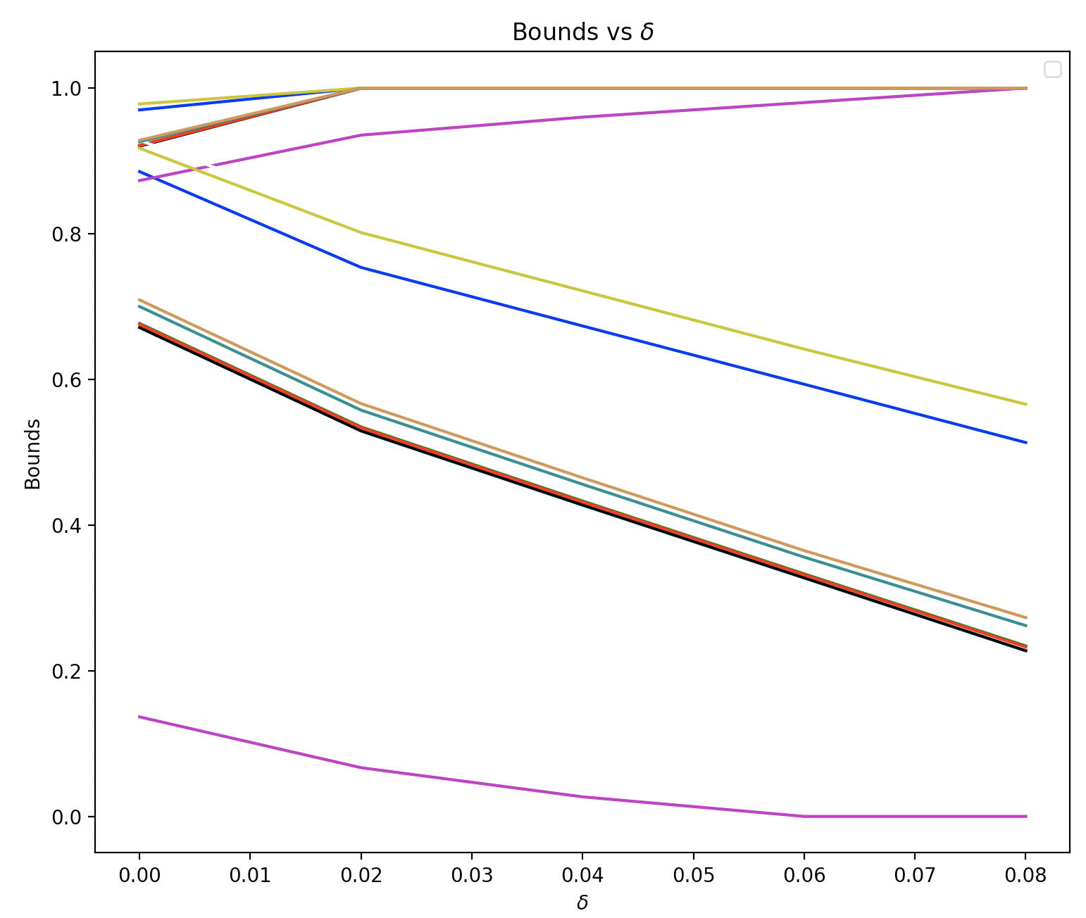
Figure 5: Lower and upper bounds vs $\delta$ for 10 instances of $\bar{p}$ in Example A. Lines of the same color denotes lower and upper bounds for the same instance.

We now extend LPs (21) and (22) to the finite data setting. Bounds in this setting can be computed by solving the following LPs:

$$\begin{array}[]{rll}\min_{q}/\max_{q}&\frac{\sum_{r\in R_{\mathcal{Q}}\cap R_{\mathcal{W}}}q_{r}}{\sum_{r\in R_{\mathcal{W}}}q_{r}}\\ \text{s.t.}&\sum_{r\in R_{v_{B}.v_{A}}}q_{r}\leq\bar{p}_{v_{B}.v_{A}}+\delta,&\forall(v_{A},v_{B}),\\ &\sum_{r\in R_{v_{B}.v_{A}}}q_{r}\geq\bar{p}_{v_{B}.v_{A}}-\delta,&\forall(v_{A},v_{B}),\\ &\sum_{r\in R}q_{r}=1,\ q\geq 0.\end{array}$$ (26)

This fractional LP can be linearized as follows.

$$\begin{array}[]{rll}\min_{\alpha,q}/\max_{\alpha,q}&\sum_{r\in R_{\mathcal{Q}}\cap R_{\mathcal{W}}}q_{r}\\ \text{s.t.}&\sum_{r\in R_{v_{B}.v_{A}}}q_{r}\leq(\bar{p}_{v_{B}.v_{A}}+\delta)\alpha,&\forall(v_{A},v_{B}),\\ &\sum_{r\in R_{v_{B}.v_{A}}}q_{r}\geq(\bar{p}_{v_{B}.v_{A}}-\delta)\alpha,&\forall(v_{A},v_{B}),\\ &\sum_{r\in R}q_{r}=\alpha,\\ &\sum_{r\in R_{\mathcal{W}}}q_{r}=1,\\ &\alpha,q\geq 0.\end{array}$$ (27)

Note that this is a linear program in $(\alpha,q)$. The previous results allow us to aggregate the $q$-variables in (27) and rewrite the LPs in terms of variables corresponding to hyperarcs.

$$\begin{array}[]{rll}\min/\max_{q,p}&\sum_{h\in H}d^{L/U}_{h}q_{h}\\ \text{s.t.}&\sum_{h:h(v_{A})=v_{B}}q_{h}\leq(\bar{p}_{v_{B}.v_{A}}+\delta)\alpha,&\forall(v_{A},v_{B}),\\ &\sum_{h:h(v_{A})=v_{B}}q_{h}\geq(\bar{p}_{v_{B}.v_{A}}-\delta)\alpha,&\forall(v_{A},v_{B}),\\ &\sum_{h\in H}q_{h}=\alpha,\\ &\sum_{h\in H:R_{h}\subseteq R_{\mathcal{W}}}q_{h}=1,\\ &\alpha,p\geq 0.\end{array}$$ (28)

Recall that the lower and upper bounds computed by solving LPs (28) incorporate additional observations of some variables in $V_{B}$. In Figure 6(a) we plot these bounds as a function of $\delta$ for the same 10 instances of $\bar{p}$, but for Example A with additional observations. (details in Appendix B). We also replicate Figure 5 with bounds computed without these additional observations for comparison; note that our bounds have shifted significantly after the observation. As in Balke and Pearl (1994), we have numerically verified the distinction between causal inference for the entire population and the sub-population consisting of units consistent with the observation.

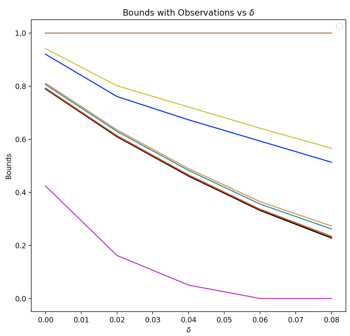
(a) Lower and upper bounds with additional observations vs $\delta$ for 10 instances of $\bar{p}$ in Example A. Lines of the same color denotes lower and upper bounds for the same instance.

(b) Lower and upper bounds without additional observations vs $\delta$ for 10 instances of $\bar{p}$ in Example A. Lines of the same color denotes lower and upper bounds for the same instance.

Figure 6: Lower and upper bounds with and without additional observations of some variables in $V_{B}$ vs $\delta$ for 10 instances of $\bar{p}$ in Example A (details in Appendix B). Note that our bounds have shifted after the observation.

6.3 Greedy Heuristic

In this section, we propose a greedy heuristic (Algorithm 5) to approximately compute the bounds for problems without additional observations when even the pruned LPs are intractable, and the bounds cannot be computed in closed form since $A\not\subseteq C(\mathcal{Q})$. Note that the bounds computed by our heuristic are guaranteed to contain the optimal bounds, and therefore, the true query value. This heuristic is motivated by the duals of LPs (5) and (7) that are defined as follows:

$$\begin{split}\alpha_{L}&=\begin{array}[t]{rll}\max_{\lambda}&\sum_{(v_{A},v_{B})\in\{0,1\}^{|A|}\times\{0,1\}^{|B|}}p_{v_{B}.v_{A}}\lambda_{v_{B}.v_{A}}\\ \mbox{s.t.}&\sum_{v_{A}\in\{0,1\}^{|A|}}\lambda_{h(v_{A}).v_{A}}\leq c_{h}^{L},&\forall h\in H.\end{array}\end{split}$$ (29)

$$\begin{split}\alpha_{U}&=\begin{array}[t]{rll}\min_{\lambda}&\sum_{(v_{A},v_{B})\in\{0,1\}^{|A|}\times\{0,1\}^{|B|}}p_{v_{B}.v_{A}}\lambda_{v_{B}.v_{A}}\\ \mbox{s.t.}&\sum_{v_{A}\in\{0,1\}^{|A|}}\lambda_{h(v_{A}).v_{A}}\geq c_{h}^{U},&\forall h\in H.\end{array}\end{split}$$ (30)

We utilize the fact that in our numerical experiments, we observed that for both dual LPs, there was always an optimal solution that only took values in the set $\{-1,0,1\}$, and the fact that in the symbolic bounds introduced by Balke and Pearl (1994) (see, also Zhang and Bareinboim (2017); Pearl (2009); Sjölander et al. (2014); Sachs et al. (2022)) the probabilities in the input data were combined using coefficients taking values in $\{-1,0,1\}$. In fact, we expect the following conjecture to be true.

Conjecture 13 (Dual Integrality)

The dual LPs in (29) and (30) have optimal solutions which only take values in $\{-1,0,1\}$.

Graph	% instances with $\alpha_{L}^{G}=\alpha_{L}$	% instances with $\alpha_{U}^{G}=\alpha_{U}$	% instances with $\epsilon_{L}\leq 10\%$	% instances with $\epsilon_{U}\leq 10\%$
Ex A	100	100	100	100
Ex B	99	86	99	94
Ex C	100	84	100	86
Ex F	100	100	100	100
Ex G	100	100	100	100

Table 4: Quality of the bounds computed by the greedy algorithm over 100 instances of Examples A, B, C, F and G (details in Appendix B). Here $\alpha_{L}^{G}$ (resp. $\alpha_{U}^{G}$) denotes the lower (resp. upper) bound computed by the greedy heuristic, $\alpha_{L}$ (resp. $\alpha_{U}$) denotes the lower (resp. upper) bound computed by solving the LP, $\epsilon_{L}=(\alpha_{L}-\alpha^{G}_{L})/\alpha_{L}$ (resp. $\epsilon_{U}=(\alpha^{G}_{U}-\alpha_{U})/\alpha_{U}$) is a measure of suboptimality of the lower (resp. upper) bound computed by the greedy heuristic.

Algorithm 5 Greedy Heuristic

Let the permutation which sorts the conditional probabilities in descending order be $i_{1},\ldots,i_{2^{|N|}}$.

Function GreedyLowerBound():

       Initialize $\lambda=-\boldsymbol{1}$.  for $j=1,..,2^{|N|}$ do

             while $\lambda$ is feasible do

                   $\lambda_{i_{j}}=\lambda_{i_{j}}+1$

            

      

Function GreedyUpperBound():

       Initialize $\lambda=\boldsymbol{1}$.   for $j=1,..,2^{|N|}$ do

             while $\lambda$ is feasible do

                   $\lambda_{i_{j}}=\lambda_{i_{j}}-1$

            

      

We tested Algorithm 5 on $100$ instances of each of the examples in Appendix B for which bounds were not available in closed form. The results reported in Table 4 are for Examples A, B, C, F and G for which the LP can be solved. We see that bounds from the greedy heuristic matches the LP bounds in most instances for these problems. Recall that one can compute the optimal bounds for Examples A, F and G only after pruning the LP. In Table 4, $\epsilon_{L}=1-\frac{\alpha^{G}_{L}}{\alpha_{L}}$ and $\epsilon_{U}=\frac{\alpha^{G}_{U}}{\alpha_{U}}-1$ denote the relative errors of the lower and upper bounds, respectively. We see that the lower bound is always within $10\%$ of the true value, whereas the upper bound is within $10\%$ for at least $86\%$ of the cases. See Appendix for the empirical distribution function of errors. Furthermore, the greedy heuristic yields non-trivial bounds for Examples D and E, where the corresponding pruned LP is too large to be solved to optimality.

7 Conclusion

In this work, we compute bounds for the expected value of some outcome variables $V_{O}$ if we intervene on variables $V_{I}$, given the values of variables $V_{A}$ are known, via linear programming. We show how to leverage structural properties of these LPs to significantly reduce their size. We also show how to construct these LPs efficiently. As a direct consequence of our results, bounds for causal queries can be computed for graphs of much larger size. We show that there are examples of causal inference problems for which bounds could be computed only after the pruning we introduce. Our structural results also allow us to characterize a set of causal inference problems for which the bounds can be computed in closed form. This class includes as a special case extensions of problems considered in the multiple confounded treatments literature (Wang and Blei, 2021; Ranganath and Perotte, 2019; Janzing and Schölkopf, 2018; D’Amour, 2019; Tran and Blei, 2017). We show that bounds for queries containing additional observations about the unit can be computed by solving fractional LPs (Bitran and Novaes, 1973). These fractional LPs are special because the denominator is restricted to be non-negative. This allows us to homogenize the problem into a LP with one additional constraint, and extend the structural results obtained for queries without additional observations. We also show the significant runtime improvement provided by our methods compared to benchmarks in numerical experiments and extend the results to the finite data setting. Finally, for causal inference without additional observations, we propose a very efficient greedy heuristic that produces very high quality bounds, and scales to problems that are several orders of magnitude larger than those for which the pruned LPs can be solved.

Appendix A Basic results

Lemma 14 (Partition of $R$)

$R=\cup_{h\in H}R_{h}$ is a partition of $R$.

Proof  Since $R_{h}\subseteq R$ for all $h\in H$, it follows that $\cup_{h\in H}R_{h}\subseteq R$. Next, we show that $R\subseteq\cup_{h}R_{h}$. Fix $\bar{r}\in R$. Then $\bar{r}\in R_{h}$ for some hyperarc $h$ such that $h(v_{A})=F_{B}(v_{A},\bar{r})$ for all $v_{A}\in\{0,1\}^{|A|}$. Thus, $R\subseteq\cup_{h}R_{h}$.

Next, suppose there exist $h_{1}\neq h_{2}$ such that $R_{h_{1}}\cap R_{h_{2}}\neq\emptyset$. Then for all $r\in R_{h_{1}}\cap R_{h_{2}}$, and all $v_{A}\in\{0,1\}^{|A|}$, we have $h_{i}(v_{A})=F_{B}(v_{A},r)$, $i=1,2$. Thus, it follows that $h_{1}(v_{A})=h_{2}(v_{A})$ for all $v_{A}\in\{0,1\}^{|A|}$. A contradiction.  

Lemma 15 (Critical Intervention Variables)

Let $G^{do(V_{I}=q_{I})}$ denote the mutilated graph after intervention $do(V_{I}=q_{I})$, i.e. variables $V_{I}$ no longer have any incoming arcs, and let $V_{C(\mathcal{Q})}$ denote the set of variables in $V_{A}\cup V_{B}$ that have a path to some variable in $V_{O}$ in $G^{do(V_{I}=q_{I})}$.Then

$$\mathbb{P}(V_{O}(V_{I}=q_{I})=q_{O}|V_{A}=q_{A})=\mathbb{P}(V_{O}(V_{I\cap C(\mathcal{Q})}=q_{I\cap C(\mathcal{Q})})=q_{O}|V_{A}=q_{A})$$

Proof  By definition, for every $V\in V_{I\setminus C(\mathcal{Q})}$, there is no directed path from $V$ to a variable in $V_{O}$ in $G^{do(V_{I}=q_{I})}$. It thus follows that they do not influence the value of $V_{O}$ in the intervention. It thus follows that $\mathbb{P}(V_{O}(V_{I}=q_{I})=q_{O}|V_{A}=q_{A})=\mathbb{P}(V_{O}(V_{I\cap C(\mathcal{Q})}=q_{I\cap C(\mathcal{Q})})=q_{O}|V_{A}=q_{A})$.  

Appendix B Examples of Causal Inference Problems

In this section, we report the causal graph structure and the data generation process for the $5$ examples in Table 1.

(a) Example A

(b) Example B

(c) Example C

(d) Example D

(e) Example E

Figure 7: Examples of Causal Inference Problems

(a) Example F

(b) Example G

Figure 8: Additional Causal Inference Problems

Example A

The causal graph for this example is display in Figure 7(a). The query is: $P(Y(X_{2}=1)=1|Z_{1}=1,Z_{2}=1)$, and data generating process used to generate the input data is given by

$$U_{A} \sim N(0,1)$$

$$U_{B} \sim N(0,1)$$

$$Z_{1} \sim \text{Bernoulli}(\text{logit}^{-1}(U_{A}))$$

$$Z_{2} \sim \text{Bernoulli}(\text{logit}^{-1}(U_{A}))$$

$$S_{1} \sim \text{Bernoulli}(\text{logit}^{-1}(U_{B}))$$

$$X_{1} \sim \text{Bernoulli}(\text{logit}^{-1}(U_{B}+S_{1}))$$

$$S_{2} \sim \text{Bernoulli}(\text{logit}^{-1}(S_{1}+U_{B}+X_{1}+Z_{2}))$$

$$X_{2} \sim \text{Bernoulli}(\text{logit}^{-1}(S_{2}+U_{B}+Z_{1}+Z_{2}))$$

$$Y \sim \text{Bernoulli}(\text{logit}^{-1}(U_{B}+S_{2}+X_{2}+Z_{2}))$$

After sampling $U_{A},U_{B},Z_{1},Z_{2}$ we compute
$\mathbb{P}(Y,X_{2},S_{2},X_{1},S_{1}|Z_{2},Z_{1})=\mathbb{P}(Y|U_{B},S_{2},X_{2},Z_{2})\mathbb{P}(X_{2}|S_{2},Z_{1},Z_{2},U_{B})\mathbb{P}(S_{2}|Z_{2},U_{B},S_{1},X_{1})\mathbb{P}(X_{1}|S_{1},U_{B})\\ \mathbb{P}(S_{1}|U_{B})$
that gives input distribution. In Section 6.3, we use the observation $\{Z_{1}=1,Z_{2}=1,Y=1\}$.

Example B

The causal graph for this example is in Figure 7(b) and the query is: $P(Y(A=1,B=1)=1|C=1,F=1)$. The data generating process used to generate the input information is as follows:

$$U_{A} \sim N(0,1)$$

$$U_{B} \sim N(0,1)$$

$$C \sim \text{Bernoulli}(\text{logit}^{-1}(U_{A}))$$

$$F \sim \text{Bernoulli}(\text{logit}^{-1}(U_{A}))$$

$$A \sim \text{Bernoulli}(\text{logit}^{-1}(C+F+U_{B}))$$

$$B \sim \text{Bernoulli}(\text{logit}^{-1}(C+F+U_{B}))$$

$$D \sim \text{Bernoulli}(\text{logit}^{-1}(A+U_{B}))$$

$$E \sim \text{Bernoulli}(\text{logit}^{-1}(A+B+U_{B}))$$

$$Y \sim \text{Bernoulli}(\text{logit}^{-1}(U_{B}+D+C+E))$$

After sampling $U_{A},U_{B},C,F$ we compute

$$\mathbb{P}(A,B,D,E,Y|C,F)=\mathbb{P}(Y|U_{B},D,C,E)\mathbb{P}(E|A,B,U_{B})\mathbb{P}(D|A,U_{B})\mathbb{P}(B|C,F,U_{B})\mathbb{P}(A|C,F,U_{B}).$$

that gives the input distribution. In Section 6.3, we use the observation $\{C=1,F=1,Y=1\}$.

Example C

The causal graph for this example is in Figure 7(c) and the query is: $P(Y(M_{1}=1)=1|W_{1}=1,W_{3}=1)$. The data generating process used to generate the input information is as follows:

$$U_{A} \sim N(0,1)$$

$$U_{B} \sim N(0,1)$$

$$W_{1} \sim \text{Bernoulli}(\text{logit}^{-1}(U_{A}))$$

$$W_{3} \sim \text{Bernoulli}(\text{logit}^{-1}(U_{A}))$$

$$T \sim \text{Bernoulli}(\text{logit}^{-1}(W_{1}+W_{3}+U_{B}))$$

$$M_{1} \sim \text{Bernoulli}(\text{logit}^{-1}(T+W_{3}+U_{B}))$$

$$M_{2} \sim \text{Bernoulli}(\text{logit}^{-1}(M_{1}+W_{1}+U_{B}))$$

$$Y \sim \text{Bernoulli}(\text{logit}^{-1}(M_{2}+U_{B}))$$

$$X_{3} \sim \text{Bernoulli}(\text{logit}^{-1}(U_{B}+Y+M_{1}+T))$$

After sampling $U_{A},U_{B},W_{1},W_{3}$ we compute

$\mathbb{P}(T,M_{1},M_{2},X_{3},Y|W_{1},W_{3})=\mathbb{P}(X_{3}|U_{B},Y,M_{1},T)\mathbb{P}(Y|M_{2},U_{B})\mathbb{P}(M_{2}|M_{1},W_{1},U_{B})\\ \mathbb{P}(M_{1}|T,W_{3},U_{B})\mathbb{P}(T|W_{1},W_{3},U_{B})$

that gives the input distribution. In Section 6.3, we use the observation $\{W_{1}=1,W_{3}=1,Y=1\}$.

Example D

The causal graph for this example is in Figure 7(d) and the query is: $P(Y(D=1)=1|E=1,F=1)$. The data generating process used to generate the input information is as follows:

$$U_{A} \sim N(0,1)$$

$$U_{B} \sim N(0,1)$$

$$F \sim \text{Bernoulli}(\text{logit}^{-1}(U_{A}))$$

$$E \sim \text{Bernoulli}(\text{logit}^{-1}(U_{A}))$$

$$A \sim \text{Bernoulli}(\text{logit}^{-1}(F+E+U_{B}))$$

$$B \sim \text{Bernoulli}(\text{logit}^{-1}(E+F+A+U_{B}))$$

$$C \sim \text{Bernoulli}(\text{logit}^{-1}(B+E+F+A+U_{B}))$$

$$D \sim \text{Bernoulli}(\text{logit}^{-1}(B+E+F+A+C+U_{B}))$$

$$Y \sim \text{Bernoulli}(\text{logit}^{-1}(E+D+U_{B}))$$

$$G \sim \text{Bernoulli}(\text{logit}^{-1}(A+B+C+D+Y+E+F+U_{B}))$$

After sampling $U_{A},U_{B},E,F$ we compute

$\mathbb{P}(G,Y,D,C,B,A|E,F)=\mathbb{P}(G|U_{B},A,B,C,D,Y,E,F)\mathbb{P}(Y|E,D,U_{B})\mathbb{P}(D|B,E,F,A,C,U_{B})\\ \mathbb{P}(C|B,E,F,A,U_{B})\mathbb{P}(B|E,F,A,U_{B})\mathbb{P}(A|E,F,U_{B})$

that gives the input distribution. In Section 6.3, we use the observation $\{E=1,F=1,Y=1\}$.

Example E

The causal graph for this example is in Figure 8 and the query is: $P(Y(C=1,F=1)=1|A=1,B=1)$. The data generating process used to generate the input information is as follows:

$$U_{A} \sim N(0,1)$$

$$U_{B} \sim N(0,1)$$

$$A \sim \text{Bernoulli}(\text{logit}^{-1}(U_{A}))$$

$$B \sim \text{Bernoulli}(\text{logit}^{-1}(U_{A}))$$

$$C \sim \text{Bernoulli}(\text{logit}^{-1}(A+B+U_{B}))$$

$$D \sim \text{Bernoulli}(\text{logit}^{-1}(A+C+B+U_{B}))$$

$$E \sim \text{Bernoulli}(\text{logit}^{-1}(A+B+U_{B}))$$

$$F \sim \text{Bernoulli}(\text{logit}^{-1}(A+C+B+D+E+G+U_{B}))$$

$$G \sim \text{Bernoulli}(\text{logit}^{-1}(U_{B}+A+B+C+D))$$

$$Y \sim \text{Bernoulli}(\text{logit}^{-1}(U_{B}+A+E+B+F))$$

After sampling $U_{A},U_{B},A,B$ we compute
$\mathbb{P}(C,D,E,F,G,Y|A,B)=\mathbb{P}(C|A,B,U_{B})\mathbb{P}(D|A,C,B,U_{B})\mathbb{P}(E|A,B,U_{B})\mathbb{P}(F|A,C,B,D,E,G,U_{B})\\ \mathbb{P}(G|A,B,C,D,U_{B})\mathbb{P}(Y|U_{B},A,E,B,F)$
that gives the input distribution. In Section 6.3, we use the observation $\{A=1,B=1,Y=1\}$.

Example F

The causal graph for this example is in Figure 8(a) and the query is: $P(Y(T_{1}=1,T_{2}=1,T_{3}=1)=1|C_{1}=1,C_{2}=1)$. The data generating process used to generate the input information is as follows:

$$U_{A} \sim N(0,1)$$

$$U_{B} \sim N(0,1)$$

$$C_{1} \sim \text{Bernoulli}(\text{logit}^{-1}(U_{A}))$$

$$C_{2} \sim \text{Bernoulli}(\text{logit}^{-1}(U_{A}))$$

$$T_{1} \sim \text{Bernoulli}(\text{logit}^{-1}(C_{1}+C_{2}+U_{B}))$$

$$T_{2} \sim \text{Bernoulli}(\text{logit}^{-1}(C_{1}+C_{2}+U_{B}))$$

$$T_{3} \sim \text{Bernoulli}(\text{logit}^{-1}(C_{1}+C_{2}+U_{B}))$$

$$Y \sim \text{Bernoulli}(\text{logit}^{-1}(U_{B}+T_{1}+T_{2}+T_{3}+C_{2}))$$

After sampling $U_{A},U_{B},C_{1},C_{2}$ we compute
$\mathbb{P}(T_{1},T_{2},T_{3}|C_{1},C_{2})=\mathbb{P}(T_{1}|C_{1},C_{2},U_{B})\mathbb{P}(T_{2}|C_{1},C_{2},U_{B})\mathbb{P}(T_{3}|C_{1},C_{2},U_{B})\mathbb{P}(Y|T_{1},T_{2},T_{3},,C_{2},U_{B})$ that gives the input distribution. In Section 6.3, we use the observation $\{C_{1}=1,C_{2}=1,Y=1\}$.

Example G

The causal graph for this example is in Figure 8(b) and the query is: $P(Y(B=1)=1|W_{1}=1,W_{2}=1)$. The data generating process used to generate the input information is as follows:

$$U_{A} \sim N(0,1)$$

$$U_{B} \sim N(0,1)$$

$$W_{1} \sim \text{Bernoulli}(\text{logit}^{-1}(U_{A}))$$

$$W_{2} \sim \text{Bernoulli}(\text{logit}^{-1}(U_{A}))$$

$$D \sim \text{Bernoulli}(\text{logit}^{-1}(W_{1}+U_{B}))$$

$$A \sim \text{Bernoulli}(\text{logit}^{-1}(W_{1}+D+U_{B}))$$

$$C \sim \text{Bernoulli}(\text{logit}^{-1}(A+D+W_{1}+U_{B}))$$

$$B \sim \text{Bernoulli}(\text{logit}^{-1}(D+C+A+W_{1}+W_{2}+U_{B}))$$

$$Y \sim \text{Bernoulli}(\text{logit}^{-1}(U_{B}+D+C+A+B+W_{1}))$$

After sampling $U_{A},U_{B},W_{1},W_{2}$ we compute
$\mathbb{P}(D,A,C,B,Y|W_{1},W_{2})=\mathbb{P}(D|W_{1},U_{B})\mathbb{P}(A|W_{1},D,U_{B})\mathbb{P}(C|A,D,W_{1},U_{B})\mathbb{P}(B|D,C,A,W_{1},W_{2},U_{B})$
$\mathbb{P}(Y|D,C,A,B,W_{1},U_{B})$
that gives the input distribution. In Section 6.3, we use the observation $\{W_{1}=1,W_{2}=1,Y=1\}$.

Appendix C Empirical CDF for Error of Greedy Heuristic

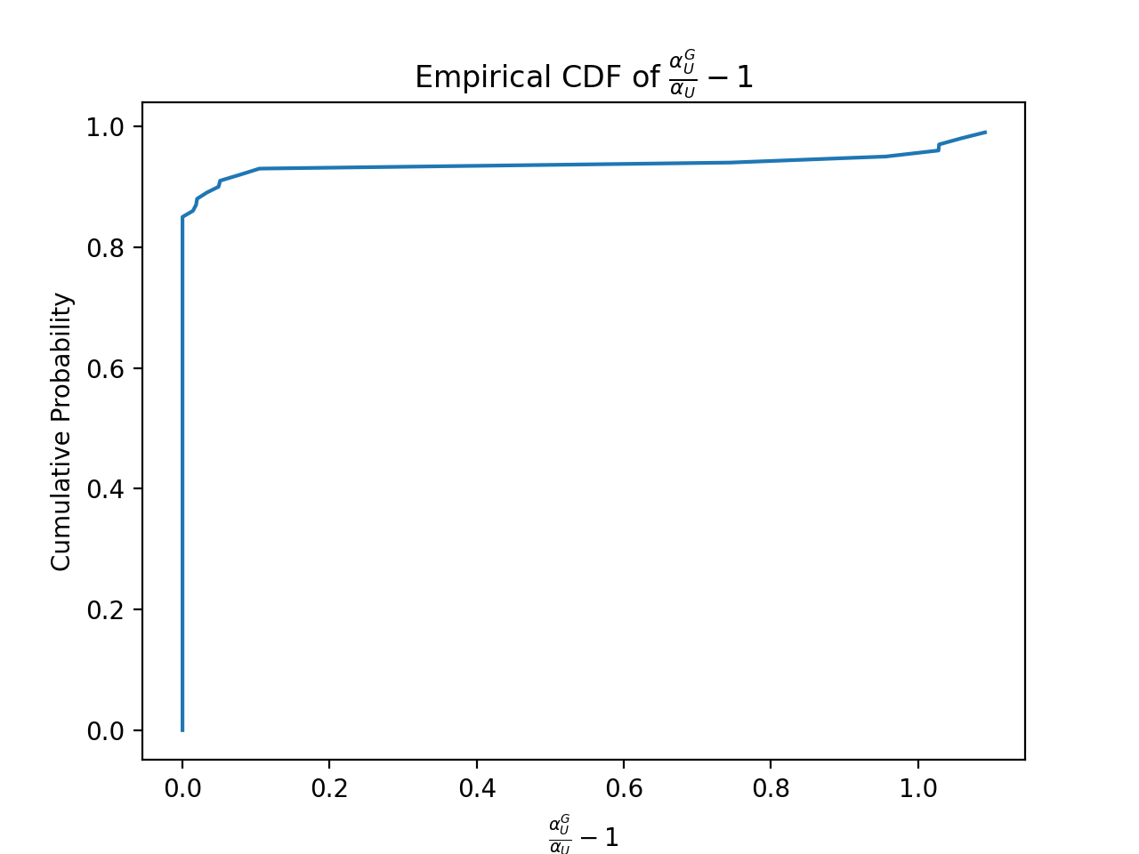
(a) Empirical CDF of the Relative Error of $\alpha_{U}$ for Example B

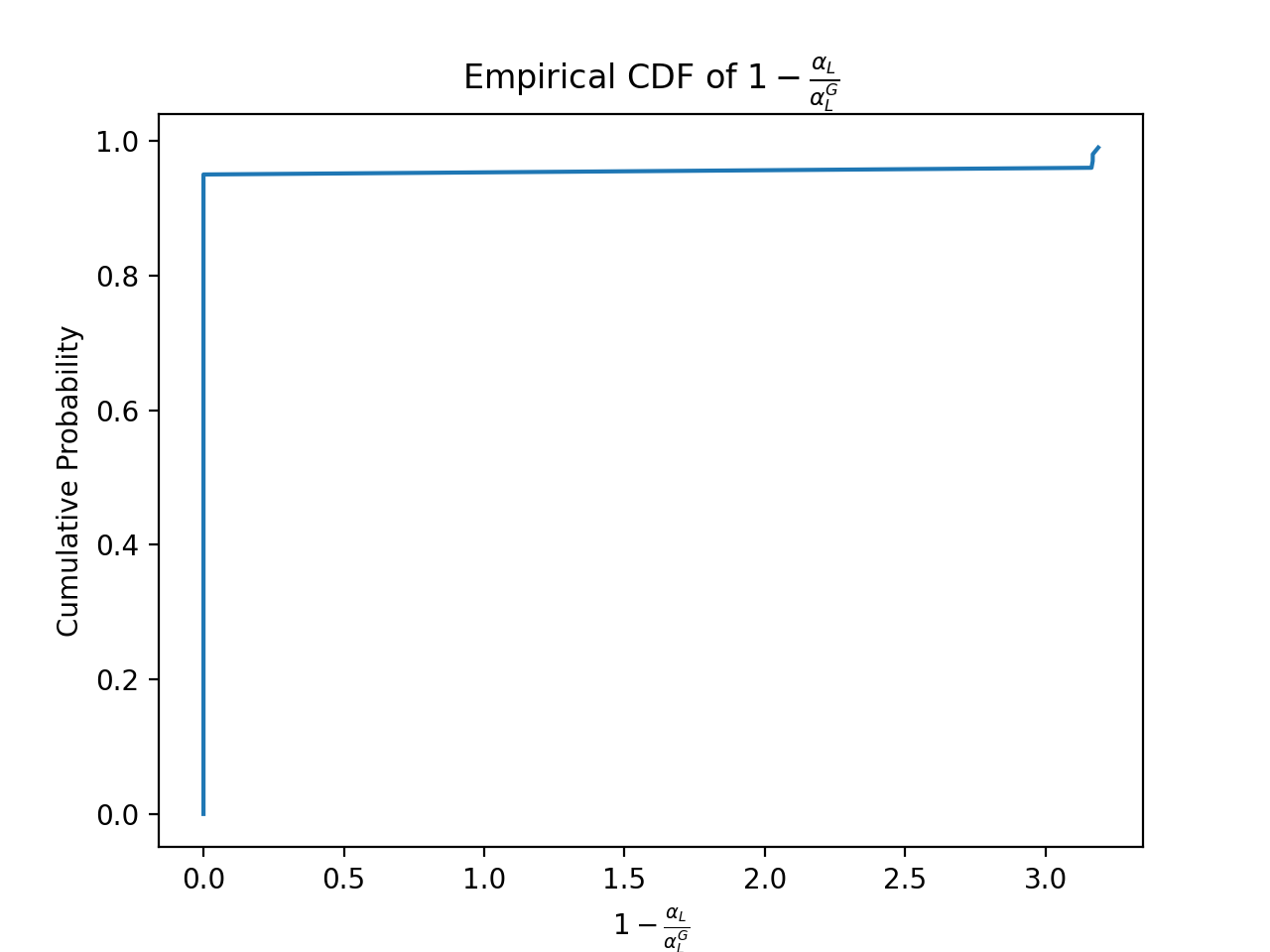
(b) Empirical CDF for Relative Error of $\alpha_{L}$ for Example B

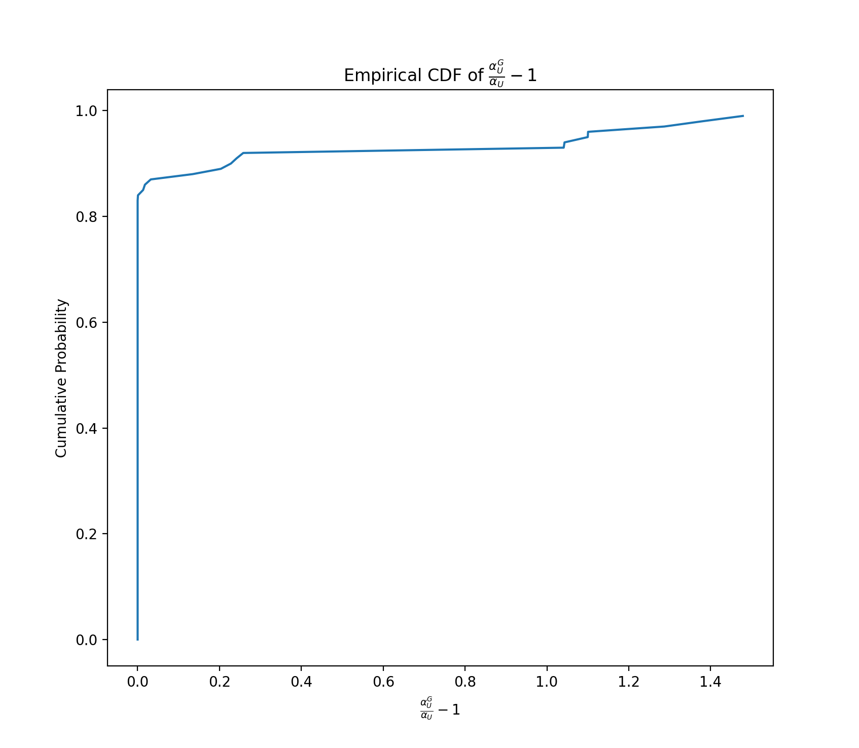
(c) Empirical CDF of the Relative Error of $\alpha_{U}$ for Example C

Figure 9: Empirical Distribution Functions of Errors for Examples

References

• Andersen (2013) Holly Andersen. When to expect violations of causal faithfulness and why it matters. Philosophy of Science, 80(5):672–683, 2013.
• Balke and Pearl (1994) A. Balke and J. Pearl. Counterfactual probabilities: Computational methods, bounds and applications. In Uncertainty Proceedings 1994, pages 46–54. Elsevier, 1994.
• Bertsimas and Tsitsiklis (1997) Dimitris Bertsimas and John Tsitsiklis. Introduction to Linear Optimization. Athena Scientific, 1st edition, 1997. ISBN 1886529191.
• Bitran and Novaes (1973) G. R. Bitran and A. G. Novaes. Linear programming with a fractional objective function. Operations Research, 21(1):22–29, 1973.
• Charnes and Cooper (1962) A. Charnes and W. W. Cooper. Programming with linear fractional functionals. Naval Research logistics quarterly, 9(3-4):181–186, 1962.
• D’Amour (2019) A. D’Amour. On multi-cause approaches to causal inference with unobserved counfounding: Two cautionary failure cases and a promising alternative. In Kamalika Chaudhuri and Masashi Sugiyama, editors, Proceedings of the Twenty-Second International Conference on Artificial Intelligence and Statistics, volume 89 of Proceedings of Machine Learning Research, pages 3478–3486. PMLR, 16–18 Apr 2019. URL https://proceedings.mlr.press/v89/d-amour19a.html.
• Duarte et al. (2021) G. Duarte, N. Finkelstein, D. Knox, J. Mummolo, and I. Shpitser. An automated approach to causal inference in discrete settings. arXiv preprint arXiv:2109.13471, 2021.
• Evans (2012) R. J. Evans. Graphical methods for inequality constraints in marginalized DAGs. In 2012 IEEE International Workshop on Machine Learning for Signal Processing, pages 1–6, 2012. doi: 10.1109/MLSP.2012.6349796.
• Finkelstein and Shpitser (2020) N. Finkelstein and I. Shpitser. Deriving bounds and inequality constraints using logical relations among counterfactuals. In Conference on Uncertainty in Artificial Intelligence, pages 1348–1357. PMLR, 2020.
• Finkelstein et al. (2021) N. Finkelstein, R. Adams, S. Saria, and I. Shpitser. Partial identifiability in discrete data with measurement error. In Cassio de Campos and Marloes H. Maathuis, editors, Proceedings of the Thirty-Seventh Conference on Uncertainty in Artificial Intelligence, volume 161 of Proceedings of Machine Learning Research, pages 1798–1808. PMLR, 27–30 Jul 2021. URL https://proceedings.mlr.press/v161/finkelstein21b.html.
• Geiger and Meek (2013) D. Geiger and C. Meek. Quantifier elimination for statistical problems, 2013. URL https://arxiv.org/abs/1301.6698.
• Imai and Jiang (2019) K. Imai and Z. Jiang. Discussion of ”the blessings of multiple causes” by wang and blei, 2019.
• Imbens and Rubin (2015) G. W. Imbens and D. B. Rubin. Causal inference in statistics, social, and biomedical sciences. Cambridge University Press, 2015.
• Janzing and Schölkopf (2018) D. Janzing and B. Schölkopf. Detecting confounding in multivariate linear models via spectral analysis. Journal of Causal Inference, 6(1):20170013, 2018. doi: doi:10.1515/jci-2017-0013. URL https://doi.org/10.1515/jci-2017-0013.
• Kilbertus et al. (2020) N. Kilbertus, M. J. Kusner, and R. Silva. A class of algorithms for general instrumental variable models. In H. Larochelle, M. Ranzato, R. Hadsell, M.F. Balcan, and H. Lin, editors, Advances in Neural Information Processing Systems, volume 33, pages 20108–20119. Curran Associates, Inc., 2020. URL https://proceedings.neurips.cc/paper/2020/file/e8b1cbd05f6e6a358a81dee52493dd06-Paper.pdf.
• Ogburn et al. (2019) E. L. Ogburn, I. Shpitser, and E. J. Tchetgen. Comment on “blessings of multiple causes”. Journal of the American Statistical Association, 114(528):1611–1615, 2019. doi: 10.1080/01621459.2019.1689139. URL https://doi.org/10.1080/01621459.2019.1689139.
• Pearl (2009) J. Pearl. Causality: Models, Reasoning and Inference. Cambridge University Press, USA, 2nd edition, 2009. ISBN 052189560X.
• Poderini et al. (2020) D. Poderini, R. Chaves, I. Agresti, G. Carvacho, and F. Sciarrino. Exclusivity graph approach to instrumental inequalities. In Ryan P. Adams and Vibhav Gogate, editors, Proceedings of The 35th Uncertainty in Artificial Intelligence Conference, volume 115 of Proceedings of Machine Learning Research, pages 1274–1283. PMLR, 22–25 Jul 2020. URL https://proceedings.mlr.press/v115/poderini20a.html.
• Ranganath and Perotte (2019) Rajesh Ranganath and Adler Perotte. Multiple causal inference with latent confounding, 2019.
• Richardson et al. (2014) A. Richardson, M. G. Hudgens, P.B. Gilbert, and J.P. Fine. Nonparametric bounds and sensitivity analysis of treatment effects. Stat Sci, 29(4):596–618, 2014. doi: 10.1214/14-STS499.
• Sachs et al. (2020) M. C. Sachs, E. E. Gabriel, and A. Sjolander. Symbolic computation of tight causal bounds. Biometrika, 103(1):1–19, 2020.
• Sachs et al. (2022) Michael C Sachs, Gustav Jonzon, Arvid Sjölander, and Erin E Gabriel. A general method for deriving tight symbolic bounds on causal effects. Journal of Computational and Graphical Statistics, pages 1–10, 2022.
• Shridharan and Iyengar (2022) Madhumitha Shridharan and Garud Iyengar. Scalable computation of causal bounds. In Proceedings of the 39th International Conference on Machine Learning, volume 162 of Proceedings of Machine Learning Research, pages 20125–20140. PMLR, 17–23 Jul 2022. URL https://proceedings.mlr.press/v162/shridharan22a.html.
• Sjölander et al. (2014) A. Sjölander, W. Lee, H. Källberg, and Y. Pawitan. Bounds on causal interactions for binary outcomes. Biometrics, 70(3):500–505, 2014. ISSN 0006341X, 15410420. URL http://www.jstor.org/stable/24538083.
• Tran and Blei (2017) D. Tran and D. M. Blei. Implicit causal models for genome-wide association studies, 2017.
• Wang and Blei (2019a) Y. Wang and D. M. Blei. The blessings of multiple causes. Journal of the American Statistical Association, 114(528):1574–1596, 2019a.
• Wang and Blei (2021) Y. Wang and D. M. Blei. A proxy variable view of shared confounding. In Marina Meila and Tong Zhang, editors, Proceedings of the 38th International Conference on Machine Learning, volume 139 of Proceedings of Machine Learning Research, pages 10697–10707. PMLR, 18–24 Jul 2021. URL https://proceedings.mlr.press/v139/wang21c.html.
• Wang and Blei (2019b) Yixin Wang and David M. Blei. The blessings of multiple causes: Rejoinder. Journal of the American Statistical Association, 114(528):1616–1619, 2019b. doi: 10.1080/01621459.2019.1690841. URL https://doi.org/10.1080/01621459.2019.1690841.
• Zhang and Bareinboim (2017) J. Zhang and E. Bareinboim. Transfer learning in multi-armed bandits: A causal approach. In Proceedings of the Twenty-Sixth International Joint Conference on Artificial Intelligence, IJCAI-17, pages 1340–1346, 2017. doi: 10.24963/ijcai.2017/186. URL https://doi.org/10.24963/ijcai.2017/186.
• Zhang and Bareinboim (2021) J. Zhang and E. Bareinboim. Bounding causal effects on continuous outcome. Proceedings of the AAAI Conference on Artificial Intelligence, 35(13):12207–12215, May 2021. URL https://ojs.aaai.org/index.php/AAAI/article/view/17449.
• Zhang et al. (2022) Junzhe Zhang, Jin Tian, and Elias Bareinboim. Partial counterfactual identification from observational and experimental data. In Kamalika Chaudhuri, Stefanie Jegelka, Le Song, Csaba Szepesvari, Gang Niu, and Sivan Sabato, editors, Proceedings of the 39th International Conference on Machine Learning, volume 162 of Proceedings of Machine Learning Research, pages 26548–26558. PMLR, 17–23 Jul 2022. URL https://proceedings.mlr.press/v162/zhang22ab.html.